Towards neural reinforcement learning for large deviations in nonequilibrium systems with memory

Abstract

We introduce a reinforcement learning method for a class of non-Markov systems; our approach extends the actor-critic framework given by Rose et al. [New J. Phys. 23 013013 (2021)] for obtaining scaled cumulant generating functions characterizing the fluctuations. The actor-critic is implemented using neural networks; a particular innovation in our method is the use of an additional neural policy for processing memory variables. We demonstrate results for current fluctuations in various memory-dependent models with special focus on semi-Markov systems where the dynamics is controlled by nonexponential interevent waiting time distributions.

1 Introduction

Large-deviation theory provides a foundational framework for stochastic systems out of equilibrium [1, 2, 3, 4, 5]. The framework defines key quantities analogous to the free energy and the entropy in equilibrium statistical physics, the scaled cumulant generating function and the rate function; these characterize fluctuations of time-averaged observables. For systems without memory (Markov processes), there is a concrete theoretical procedure based on spectral calculations to obtain the large-deviation quantities. However, except in simple toy models, this analytical procedure becomes complicated, necessitating numerical methods.

In recent years, many computational techniques have been developed to simulate and analyze rare events in systems out of equilibrium. Prominent approaches include cloning [6, 7] which is based on population dynamics of trajectories, and transition path sampling which relies on importance sampling of trajectories [8, 9]. More recently, with the objective of leveraging the efficiency of machine learning in large-deviation computations, frameworks based on reinforcement learning have been developed with successful demonstrations on several Markov systems [10, 11, 12, 13].

Notably, there has still been limited exploration of large-deviation computations for processes where memory plays an important role. A reliable computational framework arguably has more significance for non-Markov processes as memory dependence in general precludes the application of analytical methods. An implementation of cloning for memory-dependent processes can be found in [14].

In this work, we extend the reinforcement learning framework in [10] to obtain the scaled cumulant generating function in non-Markov systems. The paper is structured as follows. Section 2 introduces the nuances of memory dependence in stochastic systems via a discussion on semi-Markov processes where memory is modeled using nonexponential waiting-time distributions. Section 3 gives a brief overview of large deviations in nonequilibrium systems with a special focus on the optimal control approach used in many computational methods. Section 4 forms the core of this paper where we discuss various components of the reinforcement learning architecture. Section 5 demonstrates large-deviation applications on potentially interesting semi-Markov systems. Section 6 provides a summary and some perspectives for future work. Appendix A outlines a hidden-Markov analytical approach for checking some of the computational results, while appendices B and C give various technical details of our machine learning implementation.

2 Memory-dependent stochastic processes

We introduce here the theoretical background for the simulation and analysis of memory-dependent trajectories, central to the computational approach discussed in this work.

2.1 Semi-Markov trajectories

An accessible starting point for studying memory dependence in stochastic-systems is the semi-Markov process, which generalizes the familiar Markov process by introducing time-dependent rates corresponding to nonexponential waiting times that are renewed each time an event occurs. A simple yet illustrative example of such a processes is the semi-Markov continuous-time random-walk (CTRW) [15, 16]. The model extends the memoryless CTRW [17] by assuming that the time spent at a lattice point is governed by a nonexponential distribution and the time spent may also determine the transition probabilities. We use this CTRW example in discussions throughout this section and to showcase our computational method in section 4.6.

An elegant mathematical formalism for the analysis of the general and asymptotic solutions of semi-Markov processes (and some other non-Markov processes) is provided by the corresponding generalized Master equation, see [18, 16, 19]. However, here we restrict our attention to the trajectory formulation for semi-Markov processes, as described for example in [20].

We examine here the continuous-time path evolutions under semi-Markov dynamics of configurations $x$ in a discrete state space $\mathcal{S}$. Such paths can be constructed using probability densities $\psi_{x^{\prime},x}(\tau)$, each describing a transition from a given configuration $x$ to a new configuration $x^{\prime}$ in the infinitesimal waiting-time interval $[\tau,\tau+\mathrm{d}\tau)$. The densities follow the normalizing condition $\sum_{x^{\prime}}\int_{0}^{\infty}\psi_{x^{\prime},x}(\tau)=1$, where the subscript indicates the sum is over all allowed transitions from state $x$. The time spent in a state $x$ is given by the waiting-time distribution

$$\psi_{x}(\tau)=\sum_{x}\psi_{x,x^{\prime}}(\tau),$$ (1)

with the associated survival function

$$\varphi_{x}(\tau)=\int_{\tau}^{\infty}\psi_{x}(t)\mathrm{d}t.$$ (2)

The waiting-time distributions can be used to express the path transitions in a convenient form for simulations:

$$\psi_{x^{\prime},x}(\tau)=p(x^{\prime}|x,\tau)\psi_{x}(\tau).$$ (3)

Here $p(x^{\prime}|x,\tau)$ is a mass-function describing the probability of choosing a target configuration $x^{\prime}$ for the jump out of $x$, having waited at that configuration for time $\tau$. As shown, the jump probabilities in semi-Markov processes in general depend on the waiting time $\tau$, violating directional time independence, a necessary (but not sufficient) condition for equilibrium in semi-Markov processes [21]. Furthermore, we note that (3) can instead be written in terms of time-dependent process rates $\beta_{x^{\prime},x}(\tau)$ as

$$\psi_{x^{\prime},x}(\tau)=\beta_{x^{\prime},x}(\tau)\varphi_{x}(\tau).$$ (4)

Choosing exponential waiting-time distributions gives constant rates and the reduction to the Markov case.

The probability density of realizing a trajectory $\omega_{t_{0}}(t)$, starting at time $t_{0}$ in state $x_{0}$ and terminating at time $t$ in some state $x_{n}$ after $n$ observed transitions, in the infinitesimal intervals $[t_{k},t_{k}+\mathrm{d}t)_{k\in\{1,2,\cdots,n\}}$, may be written as

$$\sigma(\omega_{t_{0}}(t))=\varphi_{x_{n}}(t-t_{n})\psi_{x_{n},x_{n-1}}(t_{n}-t_{n-1})\times\cdots\\ \times\psi_{x_{2},x_{1}}(t_{2}-t_{1})\Psi_{x_{1},x_{0}}(t_{1}-t_{0})p_{0}(x_{0},t_{0}),$$ (5)

with the condition, $t_{0}<t_{1}<t_{2}<\cdots<t_{n}<t$. Here $p_{0}(x_{0},t_{0})$ and $\Psi_{x_{1},x_{0}}(t_{1}-t_{0})$ describe the probability of finding the process in configuration $x_{0}$ at time $t_{0}$ and the density of the trajectory up to the first state transition. The term, $\varphi_{x_{n}}(t-t_{n})$ represents the survival function indicating that no jumps out of $x_{n}$ occur until the final observation time $t$.

The description of initial conditions and the corresponding distributions require careful attention in systems with memory. In fact, for non-Markov, processes it is not sufficient to describe initial conditions just with the starting state $x_{0}$ and time $t_{0}$ but one also needs information on the history of the process before the observation begins. For instance, for the semi-Markov trajectory description in (5), $p_{0}(x_{0},t_{0})$ and $\Psi_{x_{1},x_{0}}(t_{1}-t_{0})$ also depend on how long the process has been in the state $x_{0}$ before $t_{0}$. Thus, to describe these distributions, we require the history of the trajectory before $(x_{0},t_{0})$, or alternatively, some average over all such histories. To elaborate on a particular case, if we know that the process has been in the state $x_{0}$ for some time $\tau_{h}$ before the initial time $t_{0}$, the initial density takes the form, $\Psi_{x_{1},x_{0}}(t_{1}-t_{0})=\psi_{x_{1},x_{0}}(t_{1}-t_{0}+\tau_{h})/\varphi_{x_{0}}(\tau_{h})$. Our notation suppresses these details in favor of retaining the general form of the distributions, without reference to history before $t_{0}$.

We may then use the trajectory probability densities (5) for further analysis of the dynamics. For example, the probability of ending up in a state $x\in\mathcal{S}$ at time $t$ starting from $x_{0}$ at time $t_{0}$ can be calculated as

$$p(x,t,x_{0},t_{0})=\delta_{x,x_{0}}\Phi_{x_{0}}(t-t_{0})p(x_{0},t_{0})\\ +\sum_{n=1}^{\infty}\int_{t_{0}}^{t}\int_{t_{1}}^{t}\dots\int_{t_{n-1}}^{t}\mathrm{d}t_{1}\mathrm{d}t_{2}\dots\mathrm{d}t_{n}\sum_{x_{1}...x_{n}}\delta_{x,x_{n}}\sigma(\omega_{t_{0}}(t)).$$ (6)

Here $\Phi_{x_{0}}(t-t_{0})$ is the survival function for the case where the process remains in state $x_{0}$ until the time $t$. Again, for a semi-Markov process which has been in the state $x_{0}$ for a time $\tau_{h}$ before $t_{0}$, we have $\Phi_{x_{0}}(t-t_{0})=\varphi_{x_{0}}(t-t_{0}+\tau_{h})/\varphi_{x_{0}}(\tau_{h})$.

Using the form given in (3), there is also an equivalent representation of the trajectory probability density (5) in terms of waiting-time distributions and probability mass functions,

$$\sigma(\omega_{t_{0}}(t))=\varphi_{x_{n}}(t-t_{n})p(x_{n}|x_{n-1},t_{n}-t_{n-1})\psi_{x_{n-1}}(t_{n}-t_{n-1})\times\cdots\\ \times p(x_{2}|x_{1},t_{2}-t_{1})\psi_{x_{1}}(t_{2}-t_{1})\Psi_{x_{1},x_{0}}(t_{1}-t_{0})p_{0}(x_{0},t_{0}).$$ (7)

This allows simulation via a modification of the Monte Carlo method due to Gillespie [22]. At a generic step $k$ of the algorithm, a waiting-time $\tau_{k}$ from $\psi_{x_{k}}(\tau)$ and a state transition $x_{k}\to x_{k+1}$ according to $p(x_{k+1}|x_{k},\tau_{k})$ are sampled. The procedure is repeated until a terminal time $t$ is reached.

As a concrete example, we return to the CTRW model mentioned at the beginning of this subsection. In particular, we consider a bidirectional semi-Markov CTRW on a discrete lattice. To avoid complications with infinite state space, we assume a finite lattice of size $L$ with periodic boundaries such that the state updates are modulo-$L$.

The dynamics is realized by two competing nonexponential probability densities $\psi^{+}(\tau)$ and $\psi^{-}(\tau)$ triggering the forward and backward jumps respectively. The corresponding survival functions are denoted $\varphi^{+}(\tau)$ and $\varphi^{-}(\tau)$. We assume here that both distributions are renewed after a jump out of a site occurs, i.e., all memory is lost after a transition event. One may imagine the above densities are associated with two competing clocks at each lattice site. The two clocks count down to the forward and backward transitions respectively and the transition associated with the winning clock (the one which rings first) is triggered. We then have the forward and backward transition densities

$$\psi_{x+1,x}(\tau)=\psi^{+}(\tau)\varphi^{-}(\tau),\quad\psi_{x-1,x}(\tau)=\psi^{-}(\tau)\varphi^{+}(\tau).$$ (8)

The first density gives the instance when the forward clock wins and the backward clock loses, while the second density gives the opposite scenario. From (1), the overall waiting-time distribution at a specific state of the process is then given by the combination

$$\psi_{x}(\tau)=\psi^{+}(\tau)\varphi^{-}(\tau)+\psi^{-}(\tau)\varphi^{+}(\tau).$$ (9)

The overall system survival function is $\varphi_{x}(\tau)=\varphi^{+}(\tau)\varphi^{-}(\tau)$, corresponding to no transitions occurring in a time interval of length $\tau$ at state $x$. Note, the process is homogeneous and the waiting-time distribution is independent of the state $x$. This means that the transitions at each lattice site of the CTRW ring all have the same clock structure described above. Finally, using (4), we may write the transition rates out of a state

$$\beta^{+}(\tau)=\frac{\psi^{+}(\tau)}{\varphi^{+}(\tau)},\quad\beta^{-}(\tau)=\frac{\psi^{-}(\tau)}{\varphi^{-}(\tau)},$$ (10)

and the associated probability mass functions

$$p(x+1|x,\tau)=\frac{\beta^{+}(\tau)}{\beta^{-}(\tau)+{\beta^{+}(\tau)}},\quad p(x-1|x,\tau)=\frac{\beta^{-}(\tau)}{\beta^{+}(\tau)+\beta^{-}(\tau)}.$$ (11)

The above quantities can then be utilized for trajectory simulations via (7). We will come back to this semi-Markov CTRW example to demonstrate results from our computational method in section 4.6.

2.2 Long-time limit

The trajectory perspective is useful for studying the statistical properties of various physical quantities that provide specific insights about the system. We are especially interested in the behavior of quantities over extremely long timescales, analogous to the thermodynamic limit in equilibrium statistical physics. In this work we focus on stochastic dynamics that lead to time-homogeneous processes that lead to a well-defined stationary state. In the time-homogeneous Markov case, this condition is met when the ergodic property holds [23], but non-Markov processes may need to satisfy further criteria. For semi-Markov systems, with rates in the extended state space of configurations and waiting times that do not depend on the process time, then a stationary state is guaranteed if, along with the ergodic property, the waiting-time distributions have finite moments [15, 16].

An important quantity of interest in nonequilibrium statistical physics is the time-integrated current $J(\omega(t))$, which counts directed jumps in the trajectory $\omega(t)$; here and in the following we often suppress the dependence on initial time $t_{0}$ in the notation for the trajectory. For example, in the CTRW case, one can define a current by counting all particle jumps across the system lattice with the current incremented or decremented based on whether a forward or a backward jump occurs. Alternatively, one can choose to count the current across particular bonds or a subset of bonds as we shall see in the multi-particle examples of section 5.2. These definitions are closely related and we will use the symbol $J(\omega(t))$ for a generic current with the time antisymmetric property. Note that if the system is at equilibrium, the time-averages of all currents in the system are zero. This is a sufficient condition for equilibrium in Markov systems. In the semi-Markov case, it is necessary but may not be sufficient.

For systems out-of-equilibrium, the long-time behavior of currents is often more interesting. When one has a nonequilibrium stationary state [24, 25], time-intensive currents $j=J(\omega(t))/{t}$ generically converge to typical (nonzero) values with well-defined moments for large but finite times. Fluctuations away from the typical values correspond to exponentially rare events. The study of such rare events is the main subject of this paper.

As rare events by definition occur far away from typical trajectories, observing them in simulations via the Gillespie method becomes very inefficient. One idea towards developing an efficient simulation procedure is by tilting or exponential reweighting of trajectory ensembles as suggested by the thermodynamic partition function,

$$Z(s,t)=\int e^{sJ(\omega(t))}\sigma(\omega(t))\mathrm{d\omega(t)}.$$ (12)

This reweighting procedure falls under the purview of importance sampling methods framework using the tilting procedure for simulating rare events is discussed in section 3.

Non-Markov theory, of course, extends beyond the simple semi-Markov processes considered above. For instance, process dynamics could depend on one or more hidden variables other than the waiting times. We believe that the method shown in this paper is applicable to all processes that relax to well-defined stationary dynamics in the state space including the hidden variables; this might include processes with weakly time-inhomogeneous rates (which become constant in the long-time limit). However, for non-Markov processes with time-inhomogeneous dynamics in the long-time limit, significant changes to the computational method would be required. A notable class of such processes are systems related to the elephant and Alzheimer’s random walks [26, 27], where the dynamics depends on the time-averaged current. Large fluctuation analysis for models of such type may be found, for example, in [28, 29, 30]. The extension of the neural reinforcement learning method introduced in this paper to processes of this kind is left to future work.

3 Current fluctuations

3.1 Large deviations

In Markov processes, the statistics of time-averaged quantities such as currents usually follow a large-deviation principle loosely stated as

$$\mathrm{Prob}\left(\frac{J(\omega(t))}{t}=j\right)\sim e^{-tI(j)},$$ (13)

where the symbol $\sim$ indicates logarithmic equality in the long-time limit. Here, $t$ is sometimes called the speed of the large deviation. In non-Markov processes, the large-deviation principle may be modified [30, 29] or even not exist at all. However, for a class of non-Markov systems, a large-deviation principle with linear speed does still hold and we restrict ourselves in this paper to such cases.

The rate function $I(j)$ in the large-deviation principle governs the occurrence probability of rare events, i.e., rare currents in the present case, and is a central quantity in nonequilibrium analysis. However, the rate function is in general difficult to obtain and is often computed indirectly via Legendre-Fenchel transformation of the scaled cumulant generating function, as prescribed by the Gärtner-Ellis theorem:

$$I(j)=\max_{s}\{sj-\lambda(s)\}.$$ (14)

From a thermodynamic standpoint, the scaled cumulant generating function (SCGF) is related to the partition function in (12) and is formally defined as

$$\lambda(s)=\lim_{t\to\infty}\frac{1}{t}\ln Z(s,t)=\lim_{t\to\infty}\frac{1}{t}\ln\left\langle e^{stj}\right\rangle_{\sigma(\omega(t))},$$ (15)

where the average is over trajectory probabilities $\sigma(\omega(t))$ of the process.

3.2 An optimal control approach

In the Markov case, the SCGF is the principal eigenvalue of the tilted (exponentially reweighted) form of the rate matrix governing the dynamics and for simple examples can be calculated analytically. Beyond these simple Markov cases and certainly in the non-Markov context, the SCGF may take a more complicated form, making analytical progress prohibitively difficult. Moreover, complications such as phase transitions may arise even in Markov systems [31, 32]. Large deviations in many cases can only be probed numerically, highlighting the importance of efficient computational techniques. The broad objective of most techniques referenced in this work is to obtain the SCGF through trajectories of an alternate or modified dynamics whose typical behavior corresponds to the large fluctuations of the original dynamics. The probability of a trajectory under the alternate dynamics is then given as

$$\sigma^{w}(\omega(t))=e^{sJ(\omega(t))}\frac{\sigma(\omega(t))}{Z(s,t)},$$ (16)

where the exponentially weighted trajectory probabilities are normalized by the partition function $Z(s,t)$. For Markov systems, the alternate dynamics is obtained via the Doob transform, see e.g. [33], which is utilized in cloning algorithms [7, 6].

A more general way of obtaining the alternate dynamics is by using a variational approach, as in [34], applied over a parameterized model representing the alternate dynamics. In particular, as shown in [33] the alternate dynamics is estimated via the minimization of the Kullback-Liebler divergence (KLD)

$$D_{\mathrm{KL}}(\sigma^{\theta}(\omega(t)),\sigma^{w}(\omega(t))) =\left\langle\ln\frac{\sigma^{\theta}(\omega(t))}{\sigma^{w}((\omega(t))}\right\rangle_{\sigma^{\theta}(\omega(t))}$$

$$=\left\langle-sJ(\omega(t))+\ln\frac{\sigma^{\theta}(\omega(t))}{\sigma(\omega(t))}\right\rangle_{\sigma^{\theta}(\omega(t))}+\ln Z(s,t).$$ (17)

Here, $\sigma^{\theta}(\omega(t))$ is the control distribution parametrized by $\theta$. Time averaging, taking the long-time limit and using the fact that the KLD is by definition non-negative, leads to the following bound involving the SCGF:

$$\lim_{t\to\infty}\frac{1}{t}\left\langle sJ(\omega(t))-\ln\frac{\sigma^{\theta}(\omega(t))}{\sigma(\omega(t))}\right\rangle_{\sigma^{\theta}(\omega(t))}\leq\lambda(s).$$ (18)

In other words, the SCGF is bounded from below by the quantity on the left-hand side. This bound is critical to variational methods and in section 4.2 we demonstrate that it can be used with reinforcement learning for the efficient computation of the SCGF in semi-Markov systems.

4 Computational framework

In this section we describe how to extend the reinforcement learning scheme by Rose, Garrahan and collaborators [10, 11, 12]. The reinforcement learning framework in their works aims to conduct a systematic and iterative search for atypical trajectories through the adaption of appropriately parameterized dynamics. In the case even of semi-Markov systems this becomes very complicated and may involve a large number of parameters. However, we show in this section that using multilayer neural networks, makes such complicated optimizations possible.

4.1 The reinforcement problem

At its core, reinforcement learning is an optimal control technique that uses environmental feedback in the form of rewards to evaluate the quality of actions leading to a trajectory step [35, 36]. In recent years, combining reinforcement learning with neural architectures has given rise to a number of diverse and powerful techniques [37, 38, 39].

The reinforcement learning system used in the present context takes inspiration from the soft actor-critic framework [40]. The actor-critic structure, as the name suggests, has an actor that searches the space of parameterized dynamics known as policies while a separate critic evaluates the policies by analyzing their effect on the environment. Each of these systems are then improved separately by using gradient-based techniques. Another vital characteristic of the framework used here is the entropy-regulation of the rewards [41, 40]. A KLD term akin to (3.2) regulates the rewards and conditions the learning towards the desired dynamics.

We consider the reinforcement problem on the extended state space that includes process memory. In particular, the reinforcement learning problem in the semi-Markov domain is posed as a decision process in the joint space of state configurations and waiting times. The decision process in the extended state space is Markovian and can be solved recursively. Related ideas appear in [42, 36, 43, 44].

To construct a semi-Markov decision process, we examine here the transitions $(x^{\prime},\tau^{\prime})\to(x^{\prime\prime},\tau^{\prime\prime})$ in the extended state space of configurations and waiting times, $\mathcal{S}\times\mathcal{T}$. In words, the process having waited at a configuration $x^{\prime}$ for a time $\tau^{\prime}$ chooses the new state $x^{\prime\prime}$ and the time $\tau^{\prime\prime}$ it must wait there until a new decision is made. From a trajectory standpoint, we assume that the process departs states $x^{\prime}$ and $x^{\prime\prime}$ at trajectory times $t^{\prime}$ and $t^{\prime\prime}$. We now return to denoting a trajectory starting at time $t_{0}$ and ending at time $t$ as $\omega_{t_{0}}(t)$. Then the piece of the trajectory $\omega_{t^{\prime}}(t^{\prime\prime})$ is generated by the density

$$\sigma^{\theta^{p},\theta^{q}}(\omega_{t^{\prime}}(t^{\prime\prime}))=\pi_{x^{\prime\prime}}^{\theta^{q}}(\tau^{\prime\prime})\pi^{\theta^{p}}(x^{\prime\prime}|x^{\prime},\tau^{\prime}).$$ (19)

Here $\theta^{p}$ and $\theta^{q}$ represent two independent sets of parameters labeled with superscripts $p$ and $q$. These separately construct adaptable sequential stochastic policies $\pi^{\theta^{p}}$ and $\pi^{\theta^{q}}$ controlling the jump to a new state and the new waiting-time respectively. As the parameter description allows policies to be independently updated, the learning simplifies [45]. The construction of this two-policy structure with neural networks is one of the key innovations of our method and will be explained in detail in section 4.3.

In general, the generation system described above can be used to simulate semi-Markov trajectories $\omega_{t_{0}}(t)$ with densities

$$\sigma^{\theta^{p},\theta^{q}}(\omega_{t_{0}}(t))=\varphi_{x_{n}}(t-t_{n})\pi^{\theta^{p}}(x_{n}|x_{n-1},\tau_{n-1})\times\cdots\\ \times\pi^{\theta^{q}}_{x_{2}}(\tau_{2})\pi^{\theta^{p}}(x_{2}|x_{1},\tau_{1})\pi^{\theta^{q}}_{x_{1}}(\tau)\Psi_{x_{1},x_{0}}(t_{1}-t_{0})p_{0}(x_{0},t_{0}),$$ (20)

anologous to the form given in (7). Similar to (7), $\Psi_{x_{1},x_{0}}(t_{1}-t_{0})$ and $\varphi_{x_{n}}(t-t_{n})$ are special and depend on the initial and terminal trajectory times selected. We do not explicitly define separate policies for these densities as their effect on the trajectory density is small in the long-time limit, when the waiting-time distributions are assumed to have finite moments. We use this argument later while defining the rewards in the next section. Although we focus here on semi-Markov systems, the technique presented can. in principle, be applied to other hidden-variable systems with minimal modifications.

4.2 Policy gradient

We extend the procedure used in [10] to construct an actor-critic reinforcement algorithm for semi-Markov systems. We begin by rewriting the KLD of (3.2) in terms of the two-policy decision process given in (20):

$$D_{\mathrm{KL}}(\sigma^{\theta^{p},\theta^{q}},\sigma_{w}) =\left\langle\ln\frac{\sigma^{\theta^{p},\theta^{q}}(\omega_{t_{0}}(t))}{\sigma^{w}(\omega_{t_{0}}(t))}\right\rangle_{\sigma^{\theta^{p},\theta^{q}}}$$

$$=\left\langle-sJ(\omega_{t_{0}}(t))+\ln{\frac{\sigma^{\theta^{p},\theta^{q}}(\omega_{t_{0}}(t))}{\sigma(\omega_{t_{0}}(t))}}\right\rangle_{\sigma^{\theta^{p},\theta^{q}}}+\ln{Z(s,t)}.$$ (21)

This further allows rewriting of the bound in (18) as

$$\lambda(s)\geq\lim_{t\to\infty}\frac{1}{t}\left\langle sJ(\omega_{t_{0}}(t))-\frac{\sigma^{\theta^{p},\theta^{q}}(\omega_{t_{0}}(t))}{\sigma(\omega_{t_{0}}(t))}\right\rangle_{\sigma^{\theta^{p},\theta^{q}}}.$$ (22)

We may then define the return over a specific finite trajectory,

$$R(\omega_{t_{0}}(t))=sJ(\omega_{t_{0}}(t))-\ln{\frac{\sigma^{\theta^{p},\theta^{q}}(\omega_{t_{0}}(t))}{\sigma(\omega_{t_{0}}(t))}},$$ (23)

to arrive at

$$\lambda(s)\geq\max_{\theta^{p},\theta^{q}}\{\lim_{t\to\infty}\frac{1}{t}\left\langle R(\omega_{t_{0}}(t))\right\rangle_{\sigma^{\theta^{p},\theta^{q}}}\}$$ (24)

as an optimization problem for the SCGF. Assuming $n$ transitions, a recursive optimization algorithm can be constructed by observing that the trajectory returns can broken down into piecewise rewards:

$$R(\omega_{t_{0}}(t))=\sum_{k=1}^{n}r_{k}(x_{k},\tau_{k},x_{k-1},\tau_{k-1}).$$ (25)

For a generic transition, $(x_{k-1},\tau_{k-1})\to(x_{k},\tau_{k})$, the reward may be defined as

$$r_{k}(x_{k},\tau_{k},x_{k-1},\tau_{k-1})=sJ(x_{k},x_{k-1})-\ln\frac{\pi_{x_{k}}^{\theta^{q}}(\tau_{k})\pi^{\theta^{p}}(x_{k}|x_{k-1},\tau_{k-1})}{\psi_{x_{k}}(\tau_{k})p(x_{k}|x_{k-1},\tau_{k-1})},$$ (26)

where $J(x_{k},x_{k-1})$ represents the change in the integrated current in the transition from $x_{k-1}$ to $x_{k}$. In a bidirectional random walk, for example, the current is incremented by one for a forward jump and decremented by one for a backward jump.

In continuous time, for fixed initial and final times $t_{0}$ and $t$, the number of transitions is itself a random variable. The initial and terminal rewards do not follow the form given in (26). In practice, we ignore these technical considerations, noting that the contribution of initial and final rewards to the return is small for long trajectories, at least when the waiting-time distributions have finite moments. The average reward per step by following the policies $\pi^{\theta^{q}}$ and $\pi^{\theta^{p}}$ is obtained as

$$\left\langle r(x_{k},\tau_{k},x_{k-1},\tau_{k-1})\right\rangle_{\pi^{\theta^{p}},\pi^{\theta^{q}}}$$

$$=\int_{0}^{\infty}\sum_{x_{k}}r(x_{k},\tau_{k}, x_{k-1},\tau_{k-1})\pi_{x_{k}}^{\theta^{q}}(\tau_{k})\pi^{\theta^{q}}(x_{k}|x_{k-1},\tau_{k-1})\mathrm{d}\tau_{k}.$$ (27)

We are interested here in the quantity $\left\langle R(\omega_{t_{0}}(t))\right\rangle_{\pi^{\theta^{q}},\pi^{\theta^{p}}}$, which is the average return over the trajectories simulated by fixing the policies $\pi^{\theta^{q}}$ and $\pi^{\theta^{p}}$ (taking into account the variable number of transitions). Intuitively, one can at this point directly optimize the return by applying a perturbative method. Computing the gradient of (4.2) separately with respect to parameters $\theta^{p}$ and $\theta^{q}$ gives,

$$\nabla_{\theta^{p}}D_{\mathrm{KL}}(\sigma^{\theta^{p},\theta^{q}}|\sigma^{w})=-\left\langle\sum_{k=1}^{n}\left(R(\omega_{t_{k}}(t))-\bar{b}\right)\nabla_{\theta^{p}}\ln\pi^{\theta^{p}}(x_{k}|x_{k-1},\tau_{k-1})\right\rangle_{\pi^{\theta^{p}},\pi^{\theta^{q}}}$$

$$\nabla_{\theta^{q}}D_{\mathrm{KL}}(\sigma^{\theta^{p},\theta^{q}}|\sigma^{w})=-\left\langle\sum_{k=1}^{n}\left(R(\omega_{t_{k}}(t)-\bar{b})\right)\nabla_{\theta^{q}}\ln\pi^{\theta^{q}}_{x_{k}}(\tau_{k})\right\rangle_{\pi^{\theta^{p}},\pi^{\theta^{q}}}.$$ (28)

Here the averages are taken over trajectories obtained by following the parameterized policies. The term $\bar{b}$ is an optional baseline, with possible dependence on the state, introduced to control the variance of the gradient updates. The derivation of (4.2) is similar to the derivation of the policy gradient in [10]. The above suggests a computation method using averaged returns over Monte Carlo trajectories as seen in policy-gradient methods [46]. However, computation of the above gradient is very inefficient for large trajectories.

4.3 Value gradient

A reliable strategy to minimize the variance in the policy gradients is to define a critic evaluating the value function pertaining to the system state space [35, 47, 38]. A value function maps states to the expected future returns. From an optimal control perspective, this gives the value of including a state in the controlled dynamics. We define a value function as the expected return over all trajectories departing from the joint state $(x^{\prime},\tau^{\prime})$ at some time $t^{\prime}$ and terminating at later time $t$. In the case of rare-event analysis, the value of the state $(x^{\prime},\tau^{\prime})$ may be understood as its contribution to the rare trajectory. We write the value function

$$V_{\pi^{\theta^{p}},\pi^{\theta^{q}}}(x^{\prime},\tau^{\prime},t^{\prime})=\left\langle R(\omega_{t^{\prime}}(t))\right\rangle_{\pi^{\theta^{p}},\pi^{\theta^{q}},x^{\prime},\tau^{\prime}},$$ (29)

where the average is over trajectories with departures from a particular state $x^{\prime}$ occurring in the infinitesimal interval $[t^{\prime},t^{\prime}+dt)$ after a waiting-time $\tau^{\prime}$ elapses. The value function follows the recursive Bellman principle [48, 42]

$$V_{\pi^{\theta^{p}},\pi^{\theta^{q}}}(x^{\prime},\tau^{\prime},t^{\prime})=\left\langle V_{\pi^{\theta^{p}},\pi^{\theta^{q}}}(x,\tau,t^{\prime}+\tau)+r(x,\tau,x^{\prime},\tau^{\prime})\right\rangle_{\pi^{\theta^{p}},\pi^{\theta^{q}},x^{\prime},\tau^{\prime}}.$$ (30)

Of course, the value function is not known initially and must also be evaluated while policy improvements are performed. Towards this end, the function is parameterized with $\phi$ and may be approximated via the Bellman equation (30) to give

$$\delta^{\phi}_{td}(x_{k},\tau_{k},x_{k-1},\tau_{k-1},t_{k})=V_{\phi}( x_{k},\tau_{k},t_{k}+\tau_{k})$$

$$+r(x_{k},\tau_{k},x_{k-1},\tau_{k-1})-V_{\phi}(x_{k-1},\tau_{k-1},t_{k}).$$ (31)

The term $\delta^{\phi}_{td}$ is known as the temporal-difference error [49] and can be minimized using the gradient-descent method via a mean-squared loss. A semi-gradient method [35] is used to simplify computations, fixing the parameters of the first value function to provide a target for the second value function. Given that we have parameters $\phi=\tilde{\phi}$ at a particular step of the algorithm, the target approximates the right-hand side of the Bellman equation at $\tilde{\phi}$. We then have the loss function

$$L_{v}(\tilde{\phi},\phi)= \frac{1}{2}\left\langle\sum_{k=1}^{n}\left(V_{\tilde{\phi}}(x_{k},\tau_{k},t_{k}+\tau_{k})+r(x_{k},\tau_{k},x_{k-1},\tau_{k-1})\right.\right.$$

$$\phantom{.........}\left.\left.-V_{\phi}(x_{k-1},\tau_{k-1},t_{k})|_{\phi=\tilde{\phi}}\right)^{2}\right\rangle_{\pi^{\theta^{p}},\pi^{\theta^{q}}},$$ (32)

and computing the gradient with respect to $\phi$ gives

$$\nabla_{\phi}L_{v}(\tilde{\phi},\phi)$$

$$=\left\langle\sum_{k=1}^{n}\left(V_{\tilde{\phi}}(x_{k},\tau_{k},t_{k}+\tau_{k})+r(x_{k},\tau_{k},x_{k-1},\tau_{k-1})\right.\right.$$

$$\left.\phantom{.....\sum_{k=1}^{n}}\quad\left.-V_{\phi}(x_{k-1},\tau_{k-1},t_{k})|_{\phi=\tilde{\phi}}\right)\nabla_{\phi}V_{\phi}(x_{k-1},\tau_{k-1},t_{k})\right\rangle_{\pi^{\theta^{p}},\pi^{\theta^{q}}}$$

$$=\left\langle\sum_{k=1}^{n}\delta^{\phi}_{td}(x_{k},\tau_{k},x_{k-1},\tau_{k-1},t_{k})|_{\phi=\tilde{\phi}}\nabla_{\phi}V_{\phi}(x_{k-1},\tau_{k-1},t_{k})\right\rangle_{\pi^{\theta^{p}},\pi^{\theta^{q}}}.$$ (33)

Since the target estimates the future returns we use this in (4.2). Applying the value approximation of the current-state as the baseline we may write

$$\left\langle R(\omega_{t_{k}}(t))\right\rangle_{\pi^{\theta^{p}},\pi^{\theta^{q}}}-\bar{b} =\left\langle V_{\tilde{\phi}}(x_{k},\tau_{k},t_{k}+\tau_{k})+r(x_{k},\tau_{k},x_{k-1},\tau_{k-1})\right\rangle_{\pi^{\theta^{p}},\pi^{\theta^{q}}}$$

$$-V_{\phi}(x_{k-1},\tau_{k-1},t_{k})|_{\phi=\tilde{\phi}}$$

$$=\delta_{td}^{\phi}(x_{k},\tau_{k},x_{k-1},\tau_{k-1},t_{k})|_{\phi=\tilde{\phi}},$$ (34)

giving, as in [38, 10, 11], the policy gradients in terms of the temporal-difference error:

$$\nabla_{\theta^{p}}D_{\mathrm{KL}}(\sigma^{\theta^{p},\theta^{q}}|\sigma^{w})=-\left\langle\sum_{k=1}^{n}\delta_{td}^{\phi}(x_{k},\tau_{k},x_{k-1},\tau_{k-1},t_{k})\nabla_{\theta^{p}}\ln\pi^{\theta^{p}}(x_{k}|x_{k-1},\tau_{k-1})\right\rangle_{\pi^{\theta^{p}},\pi^{\theta^{q}}}$$

$$\nabla_{\theta^{q}}D_{\mathrm{KL}}(\sigma^{\theta^{p},\theta^{q}}|\sigma^{w})=-\left\langle\sum_{k=1}^{n}\delta_{td}^{\phi}(x_{k},\tau_{k},x_{k-1},\tau_{k-1},t_{k})\nabla_{\theta^{q}}\ln\pi_{x_{k}}^{\theta^{q}}(\tau_{k})\right\rangle_{\pi^{\theta^{p}},\pi^{\theta^{q}}}.$$ (35)

4.4 Differential actor-critic

In the long-time limit, applying the reinforcement learning method leads to very large returns which causes the value function to diverge. One way to resolve this issue is to consider a differential-reward setting [35, 36, 50].

Differential reinforcement learning makes use of ergodic properties that lead to time homogeneous stationary states. In the semi-Markov case, with finite waiting-time moments, time-homogeneity of the stationary dynamics is guaranteed in the extended state space of configurations and waiting-time distributions [16]. This enables the application of differential reinforcement learning. A similar argument for the application of the method can be made when the state space is extended to include hidden variables in other non-Markov systems.

We denote the average reward as

$$\bar{r}_{\theta^{p},\theta^{q}}=\lim_{t\to\infty}\frac{1}{t}\left\langle R(\omega_{t_{0}}(t))\right\rangle_{\pi^{\theta^{p}},\pi^{\theta^{q}}},$$ (36)

which gives the following differential-return over a sample trajectory

$$R_{D}(\omega_{t_{0}}(t))=\sum_{k=1}^{n}\left(r(x_{k},\tau_{k},x_{k-1},\tau_{k-1})-\tau_{k}\bar{r}_{\theta_{\tau},\theta_{p}}\right),$$ (37)

where we have assumed that the reward structure for the first step is the same as the others and neglected the subleading contribution from the piece of the trajectory after the last transition. This allows a new definition of a convergent value function in terms of differential-rewards,

$$V(x_{0},\tau_{0})=\lim_{t\to\infty}\left\langle R_{D}(\omega_{t_{0}}(t))\right\rangle_{\pi^{\theta^{p}},\pi^{\theta^{q}}},$$ (38)

which obeys the modified Bellman condition,

$$V(x^{\prime},\tau^{\prime})=\left\langle V(x,\tau)+r(x,\tau,x^{\prime},\tau^{\prime})-\tau\bar{r}_{\theta^{p},\theta^{q}}\right\rangle_{\pi^{\theta^{p}},\pi^{\theta^{q}},x^{\prime},\tau^{\prime}}.$$ (39)

The above gives a definition for the time average of the KLD [cf. $\eqref{D_kl_2}$], which holds for any transition $(x^{\prime},\tau^{\prime})\to(x,\tau)$:

$$d_{\mathrm{KL}}=-\frac{1}{t}\left\langle V(x,\tau)+R(\omega_{t_{0}}(t))-V(x^{\prime},\tau^{\prime})\right\rangle_{\pi^{\theta^{p}},\pi^{\theta^{q}}}+\frac{1}{t}\ln Z(s,t).$$ (40)

Taking derivatives with respect to the parameters and averaging over the stationary states of the dynamics under $\pi^{\theta^{p}},\pi^{\theta^{q}}$ gives the computational gradient estimates

$$\nabla_{\theta^{p}}d_{\mathrm{KL}}=-\left\langle\delta_{dtd}(x,\tau,x^{\prime},\tau^{\prime})\nabla_{\theta^{p}}\ln\pi^{\theta^{p}}(x|x^{\prime},\tau^{\prime})\right\rangle_{\pi^{\theta^{p}},\pi^{\theta^{q}}},$$

$$\nabla_{\theta^{q}}d_{\mathrm{KL}}=-\left\langle\delta_{dtd}(x,\tau,x^{\prime},\tau^{\prime})\nabla_{\theta^{q}}\ln\pi^{\theta^{q}}(\tau|x)\right\rangle_{\pi^{\theta^{p}},\pi^{\theta^{q}}}.$$ (41)

Here $\delta_{dtd}(x,\tau,x^{\prime},\tau^{\prime})$ is the differential temporal difference error obtained from the modified Bellman equation (39) and is given as

$$\delta_{dtd}(x,\tau,x^{\prime},\tau^{\prime})=V_{\phi}(x,\tau)+r(x,\tau,x^{\prime},\tau^{\prime})-\tau\bar{r}_{\theta^{p},\theta^{q}}-V_{\phi}(x^{\prime},\tau^{\prime}).$$ (42)

As before, this may be optimized by using the value gradient obtained with an objective similar to (4.3).

The differential-reward method gives a viable actor-critic reinforcement learning scheme for long times. The policy and value parameters $\{\theta^{p},\theta^{q},\phi\}$ are updated using the gradients described above. The updates can be made online (during the algorithm run) while simulating a very long trajectory. At each step of the actor-critic algorithm, the reward is computed from the actions generated by the policies. The temporal difference is computed via the value function estimate, which is then used to update the actors and the critic. The update size is controlled by choosing learning rates $\alpha_{p},\alpha_{q},\alpha_{v}$ (typically small values of the order $10^{-4}$). Finally, at the end of every step we also update the estimate for the time-averaged rewards with some learning rate $\alpha_{\bar{r}}$, i.e., at the $i^{th}$ step of the run we have

$$\bar{r}^{i+1}_{\theta^{p},\theta^{q}}=\bar{r}^{i}_{\theta^{p},\theta^{q}}+\alpha_{\bar{r}}\delta_{dtd}.$$ (43)

The complete actor-critic reinforcement method is shown in Algorithm 1.

Algorithm 1 Two-policy differential actor-critic

Parameters Initial and terminal times $t_{0}$ and $t$; average reward $\bar{r}_{\theta^{p},{\theta^{q}}}$; temporal difference $\delta_{dtd}$, learning rates $\alpha_{\theta^{p}}$, $\alpha_{\theta^{q}}$ $\alpha_{\phi}$ and $\alpha_{\bar{r}}$; parameters of the actor networks to learn policies $\pi^{\theta^{p}}$ and $\pi^{\theta^{q}}$; parameters of the critic network to learn value function $V_{\phi}$.

Initialize Set $(x^{\prime},\tau^{\prime})$ to $(x_{0},\tau_{0}+\tau_{h})$. $x_{0}$ is a random state in the configuration space. $\tau_{h}$ is the time spent in $x_{0}$ before $t_{0}$. $\tau_{0}$ is the time spent in $x_{0}$ after $t_{0}$ until the first departure. $\tau_{0}+\tau_{h}$ is sampled from a uniform distribution. Initialize neural network parameters for the actors and the critic. Initialize starting time $t_{0}$ and starting step of the run $i=1$.

$t_{1}\leftarrow t_{0}+\tau_{0}$

while $t_{i}<t$ do

  Generate a transition $x$ with $\pi^{\theta^{p}}(x|x^{\prime},\tau^{\prime})$

  Generate a waiting-time for state $\tau$ with $\pi^{\theta^{q}}_{x}(\tau)$

  Compute $r(x,\tau,x^{\prime},\tau^{\prime})$

  Get values $V_{\phi}(x^{\prime},\tau^{\prime})$ and $V_{\phi}(x,\tau)$ from the critic

  $\delta_{dtd}\leftarrow V_{\phi}(x^{\prime},\tau^{\prime})+r(x,\tau,x^{\prime},\tau^{\prime})-\tau\bar{r}_{\theta^{p},\theta^{q}}-V_{\phi}(x^{\prime},\tau^{\prime})$

  $\theta^{p}\leftarrow\theta^{p}+\alpha_{\theta^{p}}\delta_{dtd}\nabla_{\theta^{p}}\ln{\pi^{\theta^{p}}(x|x^{\prime},\tau^{\prime}})$

  $\theta^{q}\leftarrow\theta^{q}+\alpha_{\theta^{q}}\delta_{dtd}\nabla_{\theta^{q}}\ln{\pi^{\theta^{q}}_{x}}(\tau)$

  $\phi\leftarrow\phi+\alpha_{\phi}\delta_{dtd}\nabla_{\phi}V_{\phi}(x^{\prime},\tau^{\prime})$

  $\bar{r}_{\theta^{p},\theta^{q}}\leftarrow\bar{r}{{}_{\theta}}+\alpha_{\bar{r}}{\delta_{dtd}}$

  $x,\tau\leftarrow x^{\prime},\tau^{\prime}$

  $t_{i+1}\leftarrow t_{i}+\tau$

  $i\leftarrow i+1$

end while

4.5 Neural architectures

Our multi-agent reinforcement learning architecture consists of two actors and a common critic. The components are constructed using neural networks, which have shown promise as representational frameworks and have now become the standard in modern reinforcement learning methods [51, 38, 46, 39]. A neural network is a universal approximator that learns complicated functions [52, 53]. Structurally, the basic feed-forward neural network unit performs a weighted sum of the input and applies an activation function such as the hyperbolic tangent to generate non-linearity. Then, several layers of such units are stacked to create a connected graph, forming the multilayered feed-forward neural network. Mathematically, the structure is a composition of functions that apply a complicated series of transformations to the input vector to generate an output. Thus, an $l$-layered neural network with input $\mathbf{x}$ performs the weighted transformations, $\mathbf{f}^{\theta}(\mathbf{x})=\mathbf{g}_{l}^{\theta_{l}}(\mathbf{g}^{\theta_{l-1}}_{l-1}(\cdots\mathbf{g}_{1}^{\theta_{1}}(\mathbf{x})))$ to give the output $\mathbf{y}^{\theta}$.

Next, we explain the role of neural networks in our actor-critic method. We start with the construction of the policies. Although we draw inspiration from recent actor-critic reinforcement learning literature [40, 38, 39], a deeper description is warranted due to the complexity introduced by the inclusion of memory. The policy $\pi^{\theta^{p}}(x|x^{\prime},\tau^{\prime})$ is a probability mass function determining the jumps to new reachable configurations $x$, given that $(x^{\prime},\tau^{\prime})$ are the current configuration and the waiting time. The policy is constructed by applying a so-called softmax function to the outputs of a multi-layered neural network. The softmax function performs a normalizing operation to give a probability mass function. To be concrete, given that the vector $\mathbf{y}^{{\theta}^{p}}$ is the output of an $l$-layered neural network with input $(x^{\prime},\tau^{\prime})$, the $i^{\mathrm{th}}$ component of the softmax function

$$\mathrm{softmax}_{i}(\mathbf{y}^{\theta^{p}})=\frac{e^{(y^{\theta^{p}})_{i}}}{\sum_{i}e^{(y^{\theta^{p}})_{i}}},$$ (44)

gives the corresponding component of the probability mass function $\pi^{\theta^{p}}(x|x^{\prime},\tau^{\prime})$, describing the jumps. Here $(y^{\theta^{p}})_{i}$ represents the $i^{\mathrm{th}}$ component of the output vector $\mathbf{y}^{{\theta}^{p}}$.

The structure of $\pi_{x}^{\theta^{q}}(\tau)$ is slightly more complicated as this represents a non-trivial probability density with a positive support. A popular method to construct such complicated densities is by using a mixture-density network [54, 55], where the neural network learns the parameters of a mixture of known distributions. In the present case, the network learns a weighted mixture of gamma densities [56, 57], which generates the waiting-time distributions. These gamma-distribution mixtures are dense on the positive real line and even a small number of mixture components can be used to create a rich variety of distributions with positive support [57].

In general, a gamma distribution $\gamma_{a,\beta}(\tau)$, with scale parameter $a$ and rate parameter $\beta$ is given by the function

$$\gamma_{a,\beta}(\tau)=\frac{1}{\Gamma(a)}\beta^{a}\tau^{a-1}e^{-\beta\tau},$$ (45)

where $\Gamma(a)$ is the gamma function calculated at the value $a$. The gamma-mixture density is a weighted sum of such gamma distributions. The weights are normalized and form a probability mass function. The gamma mixture is thus given by

$$\mathrm{Mixture}(\tau)=\sum_{i}w_{i}\gamma_{a_{i},\beta_{i}}(\tau)$$ (46)

where the $w_{i}$ are the normalized weights.

Here the parameters of the gamma mixture are given by a neural network with input $x$. The network we use branches to give three output vectors $(\mathbf{y}^{\theta^{q}}_{w},\mathbf{y}^{\theta^{q}}_{a},\mathbf{y}^{\theta^{q}}_{\beta})$ representing the weights, scales and rates of the gamma mixture respectively. We finally have

$$\pi^{\theta^{q}}_{x^{\prime}}(\tau)=\sum_{i}\mathrm{softmax}_{i}(\mathbf{y}_{w}^{\theta^{q}})\gamma_{(y_{a}^{\theta^{q}})_{i},(y_{\beta}^{\theta^{q}})_{i}}(\tau),$$ (47)

representing the gamma-distribution mixture. The softmax operation is the same as the one described in (44). The terms $(y_{a}^{\theta^{q}})_{i}$ and $(y_{\beta}^{\theta^{q}})_{i}$ represent the $i^{\mathrm{th}}$ component of the vectors $\mathbf{y}^{\theta^{q}}_{a}$ and $\mathbf{y}^{\theta^{q}}_{\beta}$ respectively. We thus generate powerful densities to represent waiting-time distributions of the modified dynamics. As an aside, other density-generation methods such as normalizing flows [9, 58, 59] could be used instead.

Our policy structure allows the inclusion of hidden variables, beyond just waiting times. Since the policies distill information from memory to generate decisions, they takes on a role analogous to context networks used in machine learning, especially in large language generation models [60, 61, 62]. We seek to explore this connection further in future work.

The value function is approximated using a standard multi-layered feed-forward neural network with weight parameters $\phi$. The inputs to the network are the configuration and the corresponding waiting time. The network outputs an estimation of the value for the inputs given. The actor and critic parameters $\theta^{p},\theta^{q},\phi$ are updated using the stochastic gradient descent method, following Algorithm 1. In practice, the gradients performed on neural networks use the modified stochastic gradients given by the ADAM updates [63].

In neural networks, new information interferes with previously learnt weights in a phenomenon known as catastrophic forgetting [64]. This poses a major problem, especially in many reinforcement learning applications where data is obtained sequentially. Constructing neural policies from orthogonal subspaces offers some protection against catastrophic forgetting, which seems to be another advantage of the two-policy structure presented above. Catastrophic forgetting is further mitigated by performing gradient descent over a parallel batch of samples, i.e., batch learning. In the present context, selecting a batch size corresponds to selecting the number of sample trajectories for parallel evaluation. Another popular method that could be incorporated in our architecture for reducing interference would be to use a so-called replay buffer [65]. The networks would then trained on randomly chosen samples from the buffer instead of just the immediate previous samples.

Before applying the actor-critic reinforcement learning method in earnest in section 5, we next apply it to the testcase of current fluctuations in the semi-Markov CTRW.

4.6 Example: semi-Markov CTRW

To demonstrate the reinforcement learning method, we consider again the semi-Markov CTRW of section 2.1. The individual waiting-time densities, $\psi^{+}(\tau)$ and $\psi^{-}(\tau)$, of the forward and backward processes in (9) are now taken to be gamma distributions $\gamma_{a,\beta^{+}}(\tau)$ and $\gamma_{a,\beta^{-}}(\tau)$ with the form shown in (45). The associated survival functions $\varphi^{+}(\tau)$ and $\varphi^{-}(\tau)$ contain the corresponding upper-incomplete gamma functions. Both distributions are here assumed to have the same value for the scale parameter, $a=2$. In this case, semi-analytical calculations are still possible using an equivalent hidden Markov model as the gamma distribution is an example of a phase-type distribution [66, 67] (see appendix A). This makes the model an ideal testcase for our algorithm.

The results in figure 1 show excellent agreement of the reinforcement learning with the analytical approach. The reinforcement learning also directly gives the modified dynamics. Figure 1(b) shows that the average-reward (the SCGF estimate) converges rapidly to the true value as the process time increases, with slower convergence for values of $s$ corresponding to fluctuations further away from the mean. Preliminary investigations suggest comparable performance with the cloning algorithm of [14].

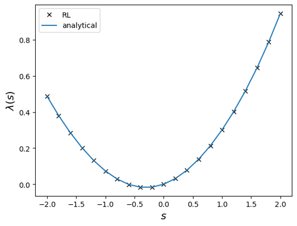
(a)

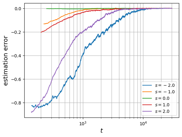
(b)

Figure 1: Current fluctuations in semi-Markov CTRW with $(a,\beta^{+},\beta^{-})=(2,0.6,0.4)$. (a) Crosses show the estimated SCGF from the actor-critic reinforcement learning algorithm with $t=20\,000$ (and $t_{0}=0$); solid line shows long-time result from equivalent hidden Markov model. (b) Colored lines show convergence of the estimated SCGF to the true asymptotic value, at different values of the conjugate variable $s$, with respect to process time $t$.

5 Applications

In this section, we demonstrate the neural reinforcement learning method on more complicated single and multi-particle systems with memory.

5.1 Memory-induced ratchets

In thermodynamics, ratchet models demonstrate symmetry-breaking mechanisms which may appear surprising and push a system out of equilibrium [68, 69, 70]. A paradigmatic example is the flashing ratchet, see for example [71, 72], where a sawtooth potential is periodically applied to Brownian particles. The particles are trapped in the sawtooth well when the potential is switched on while they diffuse freely when the potential is switched off. In such a system, the asymmetry of the sawtooth potential induces a nonzero current.

A recent area of interest is the examination of ratchet effects in self-propelling systems or active matter. For example, nonzero currents are generated in the run-and-tumble dynamics with equally distributed tumbles by applying an asymmetric external potential as in the flashing ratchet [73, 74]. Here, we introduce another type of ratchet which does not need an external potential. Instead, memory creates asymmetry in the dynamics and a nonzero current is generated.

We consider here the case where a particle propagates on a one-dimensional periodic lattice with random flips in its orientation. The model is comparable to the CTRW example with periodic boundaries. However, here the particle is constrained to move in a particular direction (a run) until a shift in directional polarity (a tumble) occurs. The system is easily visualized by the three site ring in figure 2.

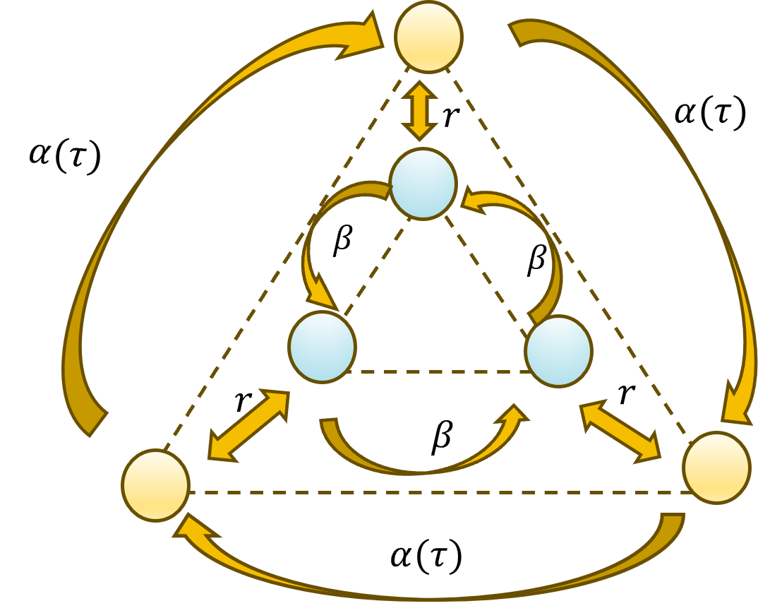
Figure 2: Representation of the memory-induced ratchet on a three-site ring. The outer ring shows the forward semi-Markov transitions. The inner ring shows the backward Markov transitions. The particle switches between the rings with constant transition rate $r$.

As in the CTRW case, since all the sites are identical, the dynamics of the current (net number of clockwise jumps) does not depend on the number of sites in the ring. In figure 2, the outer and inner rings show the forward and backward orientated dynamics respectively. A change in orientation is represented by a jump between the rings.

The system is controlled by three stochastic clocks associated with the forward jump, backward jump and the next directional change respectively. If all three clocks are exponentially distributed then a nonzero current is only possible when the means of the forward and backward distributions are different. However, even if the two distributions have the same mean, it can be shown that nonzero currents may be generated as long as the forward and backward clocks follow different distributions. This is the ratchet effect. We save the detailed examination of this effect for future work; here we concentrate on computing the current fluctuations.

As a minimal model we take just one of the clocks as nonexponential. Without loss of generality, we assume that the forward clock corresponds to a time-varying rate $\alpha(\tau)=\psi^{\alpha}(\tau)/\varphi^{\alpha}(\tau)$, where $\psi^{\alpha}(\tau)$ is a nonexponential distribution and $\varphi^{\alpha}(\tau)$ is the associated survival function. The distribution of the clocks triggering the backward jump and the reorientations are exponential with constant rates $\beta$ and $r$ respectively. We stress that the system moves only in one direction until a reorientation event occurs, differentiating the model from the bidirectional CTRW of section 4.2. The waiting times of the system during the forward and backward phases are respectively given as

$$\psi_{x^{+}}(\tau)=\psi^{\alpha}(\tau)e^{-r\tau}+re^{-r\tau}\varphi^{\alpha}(\tau),\quad\psi_{x^{-}}(\tau)=(r+\beta)e^{-(r+\beta)\tau}.$$ (48)

The computational framework of the previous section was applied to obtain the SCGF of the currents in this system for certain choices of phase-type distributions for the forward clock. The results are shown in figure 3. The plots show good agreement with the analytical approach via equivalent hidden Markov models (see appendix A). The SCGF also indirectly shows the nonzero mean current in the system and its direction. Specifically, the mean current is given by the slope of the SCGF computed at the point where the conjugate variable $s$ is zero. Choosing the forward distribution as a hypoexponential gives a negative average current as shown by inset in figure 3(a). Alternatively, when a hyperexponential distribution is chosen, the inset plot of figure 3(b) shows that a positive current is observed.

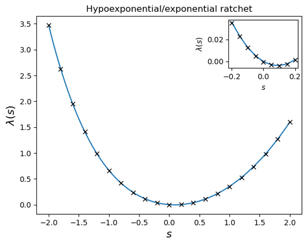
(a)

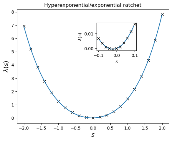
(b)

Figure 3: SCGF for currents in memory-induced ratchet systems with nonexponential distribution for forward clock and exponential distribution with same mean for backward clock. Crosses show results from reinforcement learning ($t=20\,000$, $t_{0}=0$); lines show predictions from equivalent hidden Markov models. (a) Hypoexponential distribution for forward clock, with parameters $(\alpha_{1},\alpha_{2})=(1,2)$; exponential distribution for reorientation with rate $r=1$. (b) Hyperexponential distribution for forward clock where density is a weighted sum of two equiprobable exponential distributions with rates $(\alpha_{1},\alpha_{2})=(1,2)$; exponential distribution for reorientation with rate $r=2$.

5.2 Memory-dependent totally asymmetric exclusion processes

In this section, we move beyond single-particle dynamics and show how to apply the reinforcement learning framework to multi-particle systems. In particular, we choose the well-known asymmetric exclusion process (ASEP) [75] for our demonstrations. The ASEP is an example of an out-of-equilibrium interacting particle system on a one-dimensional lattice. At any given time, a lattice site is allowed to be occupied by at most one particle. When the particle dynamics is unidirectional, the system is known as the totally asymmetric exclusion process (TASEP). We will be particularly interested in the open-boundary version of the model where it has been shown that the bond currents even in the Markov case display rich statistical behavior [76]. Here we look at currents in memory-dependent TASEPs in the vein of [14, 29, 77]. Figure 4 shows such a system.

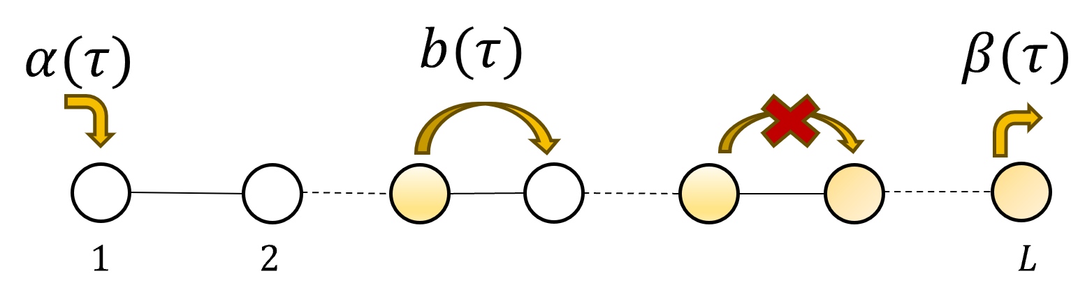
Figure 4: Memory-dependent TASEP with particles indicated by colored circles. In general, the arrival, bulk and departure processes are non-Markovian with time-varying rates. Arrows encode the exclusion rules; a particle is only allowed to enter a site when it is unoccupied.

The dynamics of an $L$-site TASEP is described by transitions in the state space $\mathcal{S}$ where each configuration is represented by a vector $\boldsymbol{\eta}$ with $L$ elements. When a lattice site is occupied, the corresponding component of the configuration vector $\boldsymbol{\eta}$ takes the value one, while it is zero when the site is vacant. We introduce memory dependence by considering that the waiting times at each configuration follow a nonexponential distribution. We denote the nonexponential distributions giving the waiting times of arrivals, bulk transitions and departures by $\psi^{\alpha}(\tau)$, $\psi^{b}(\tau)$ and $\psi^{\beta}{(\tau)}$ respectively. The corresponding survival functions $\varphi^{\alpha}(\tau)$, $\varphi^{\beta}(\tau)$ and $\varphi^{b}(\tau)$ give the individual rates

$$\alpha(\tau)=\frac{\psi^{\alpha}(\tau)}{\varphi^{\alpha}(\tau)},\quad\beta(\tau)=\frac{\psi^{\beta}(\tau)}{\varphi^{\beta}(\tau)},\quad\ b(\tau)=\frac{\psi^{b}(\tau)}{\varphi^{b}(\tau)}.$$ (49)

A useful method to track this system is to again imagine stochastic clocks that trigger the corresponding transitions. In the non-Markov TASEP, it is important to distinguish between attaching clocks to the site and attaching the clocks to the particles, as the choice may lead to different dynamics. We consider that a clock is only active when its associated transition is allowed. Explicitly, the exclusion rules give the following conditions: (i) the clock for the arrivals is only active when the first site is empty, (ii) a clock for a transition out of a site in the bulk is only active when that site is occupied and the next site is vacant (iii) the clock for the departures is active as long as the last site is occupied. When a transition associated with a clock occurs, the clock becomes inactive. When the transition is next allowed, the clock is reset and becomes active again.

Given that $\tau^{0}$, $\tau^{L}$ and $\tau^{i}$ (for $i\in\{1,2,\dots,L-1\}$) are the times since the arrival, departure and bulk-transition clocks have been active, the combined waiting-time distribution at a configuration $\boldsymbol{\eta}$ of the memory-dependent TASEP is

$$\psi_{\boldsymbol{\eta}}( \tau|\tau^{0},\tau^{1},...,\tau^{L})$$

$$= \left((1-\eta_{1})\frac{\psi^{\alpha}(\tau+\tau^{0})}{\varphi^{\alpha}(\tau+\tau^{0})}+\sum_{i=1}^{L-1}\eta_{i}(1-\eta_{i+1})\frac{\psi^{b}(\tau+\tau^{i})}{\varphi^{b}(\tau+\tau^{i})}+\eta_{L}\frac{\psi^{\beta}(\tau+\tau^{L})}{\varphi_{\beta}(\tau+\tau^{L})}\right)$$

$$\times\mathrm{exp}\left((1-\eta_{1})\ln\frac{\varphi^{\alpha}(\tau+\tau^{0})}{\varphi^{\alpha}(\tau^{0})}+\sum_{i=1}^{L-1}\eta_{i}(1-\eta_{i+1})\ln\frac{\varphi^{b}(\tau+\tau_{i})}{\varphi^{b}(\tau^{i})}\right.$$

$$\phantom{0000000000}\left.+\eta_{L}\ln\frac{\varphi^{\beta}(\tau+\tau^{L})}{\varphi^{\beta}{(\tau^{L})}}\right).$$ (50)

Here $\eta_{i}$ (for $i\in\{1,2,\cdots,L\}$) are the elements of the vector $\boldsymbol{\eta}$.

The configuration space of multi-particle systems generally scales exponentially with the number of sites. For example, in the open-boundary $L$-site exclusion process discussed above, the state space contains $2^{L}$ configurations, leading to a drop in efficiency of optimization methods due to the well-known curse of dimensionality [78]. Neural networks have allowed the application of reinforcement learning in large systems [37, 51, 38, 39] by adopting specialized neural units such as recurrent neural networks (RNNs) and convolution neural networks (CNNs) commonly used in other machine learning domains including image, speech and natural language processing [79, 80, 81, 61, 53]. We will use networks based on the so-called gated recurrent unit (GRU), an RNN variant, for handling large state spaces in the memory-dependent TASEP of section 5.2.2 (see Appendix B for more details).

5.2.1 Two-site TASEP with gamma-distributed waiting times

We first showcase the reinforcement learning method for a minimal exclusion process on just two sites. The system dynamics is governed by three memory-dependent transitions: the arrival into the first site, a (bulk) transition from the first site into the second, and the departure from the second site. We choose gamma-distributed waiting times (with scale parameter $a=2$) for each transition, motivated by the biological system in [77] where gamma distributions have been used to model ribosome dwell times.

The combined waiting-time distribution, is then obtained from (5.2) with $i=2$ and the relevant gamma distributions for the individual transitions. Focusing now on the arrival currents (by weighting jumps into the system by $e^{s}$), we computed the SCGF with the reinforcement learning algorithm. The results in figure 5 again show excellent agreement with the analytical approach based on hidden Markov models (see appendix A). Note that to apply the reinforcement learning method, the extended state space must also include the times since each of the arrival, bulk and departure clocks have been active before the process entered the present configuration. In practice, we track the state space $(\boldsymbol{\eta},\tau+\tau^{0},\tau+\tau^{1},\tau+\tau^{2})$, with implicit dependence on $\tau$, to apply Algorithm 1.

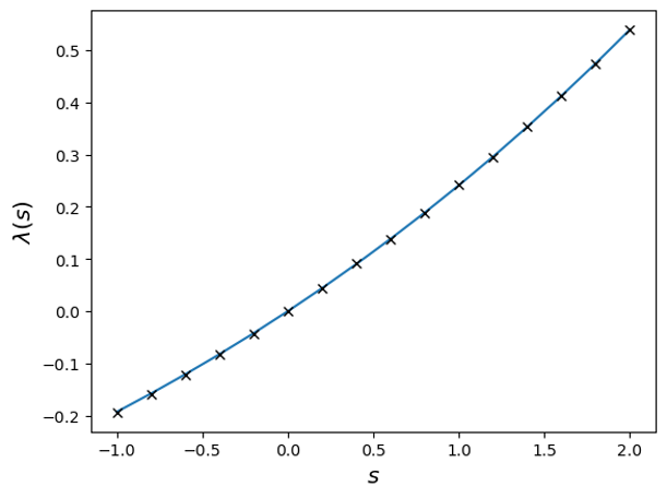
Figure 5: SCGF of arrival currents in two-site gamma TASEP, with $(a,\alpha,b,\beta)=(2,2,1,0.8)$. Here $a$ is the scale parameter for all the gamma waiting-time distributions, while $\alpha$, $b$ and $\beta$ are separate rate parameters for the arrival departure and bulk transitions respectively. Crosses are results from the reinforcement learning method ($t_{0}=0$, $t=50\,000$) and solid line is the prediction from the equivalent hidden Markov model.

5.2.2 Many-site TASEP with gamma-distributed arrival times

We conclude this section with a preliminary investigation of the neural reinforcement learning method for large systems, by extending the semi-Markov TASEP beyond two sites. To simplify calculations, we now consider that only the waiting times of the arrivals into the system are nonexponential and that all other transitions remain Markovian. We again choose a gamma distribution, with scale parameter $a=2$, to model the waiting times of the arrivals into the system. Choosing Markovian rates for bulk and departure transitions as $b$ and $\beta$ respectively, the expression (5.2) giving the combined waiting time at each configuration of the process reduces to

$$\psi_{\boldsymbol{\eta}}( \tau|\tau^{0})$$

$$= \left((1-\eta_{1})\frac{\psi^{\alpha}(\tau+\tau^{0})}{\varphi^{\alpha}(\tau+\tau^{0})}+\sum_{i=1}^{L-1}\eta_{i}(1-\eta_{i+1})b+\eta_{L}\beta\right)$$

$$\times\mathrm{exp}\left((1-\eta_{1})\ln\frac{\varphi^{\alpha}(\tau+\tau^{0})}{\varphi^{\alpha}(\tau^{0})}-\left(\sum_{i=1}^{L-1}\eta_{i}(1-\eta_{i+1})b+\eta_{L}\beta\right)\tau\right),$$ (51)

where $\psi^{\alpha}(\tau+\tau^{0})$ and $\varphi^{\alpha}(\tau+\tau^{0})$ now describe a gamma distribution and its corresponding survival function. As in the previous example, counting the fluctuations of currents into the system involves weighting of the arrivals by the factor $e^{s}$.

Figure 6 shows the SCGF computed for different system sizes: $L=2$, $L=10$ and $L=64$. For $L=2$ and $L=10$, the theoretical results for comparison were obtained via an analytical approach involving the exact diagonalization of equivalent hidden-Markov models, similar to the procedure in appendix A, but with the application of tensor products to simplify calculations for $L=10$. The SCGF calculations using the exact diagonalization method become difficult beyond $L=10$. However, significantly, the neural reinforcement learning still produces results for $L=64$ demonstrating the potential of this method for application to large systems, much beyond the scope of exact diagonalization.

Next we briefly comment on the physics of the system to interpret the SCGF in figure 6 and to justify that the $L=64$ results are reasonable. First note that we deliberately choose the parameters of the gamma distribution such that the rate of arrivals is much smaller than the bulk and the departure rates. This means that the stationary occupancy of the first site is low and the mean arrival current is expected to be asymptotically independent of the system size, just as in the low-density regime of the corresponding Markovian model [76]. The modified dynamics for nonzero $s$ effectively involves altering the rate of arrivals due to the weighting $e^{s}$. For small-magnitude $s$ (fluctuations close to the mean), figure 6 shows that the curves for $L=2$, $L=10$ and $L=64$ are indeed essentially indistinguishable. The same is true for large negative $s$, corresponding to reducing the effective rate of arrivals. On the other hand, for large positive values of $s$, the effective arrival rates become comparable to the other rates and the SCGF becomes more strongly dependent on the system size. Nevertheless, just as in the Markovian model we expect convergence to an $L$-independent limiting form. The close agreement of $L=64$ and $L=10$ in the numerical results is consistent with this intuition. Furthermore, the SCGF appears to become linear for large values of $s$ (with slope approximately $b/4$) which is indicative of a dynamical phase transition to a maximal-current phase, as seen in the Markovian case. Of course, these results are not surprising considering that only the arrivals are memory-dependent. However, they do evidence the reliability of neural reinforcement learning for this type of large system.

The reinforcement learning was implemented on the extended state space $(\boldsymbol{\eta},\tau,\tau^{0})$: the lattice configuration, the waiting time at the configuration and a memory variable indicating the time since the arrival clock has been active before entering the current configuration. The optimal transitions $(\boldsymbol{\eta^{\prime}},\tau^{\prime},\tau^{\prime 0})\to(\boldsymbol{\eta},\tau,\tau^{0})$ can be learnt by policies of form $\pi^{\theta^{p}}(\boldsymbol{\eta}|\boldsymbol{\eta^{\prime}},\tau^{\prime},\tau^{0})$ and $\pi_{\boldsymbol{\eta},\tau^{0}}^{\theta^{q}}(\tau)$. The first policy updates the configuration and the arrival clock memory while the second policy generates the waiting time in the new configuration. With this policy structure, Algorithm 1 of section 4.4 can be directly applied on the extended state space. For this more complicated model, the neural reinforcement learning method was carried out using recurrent neural networks, details of which are presented in appendix B.

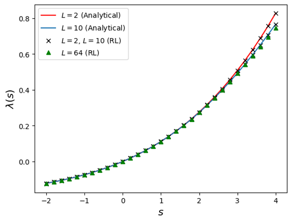
Figure 6: SCGF of arrival currents in TASEP with gamma-distributed arrival times for system sizes, $L=2$, $L=10$ and $L=64$. All cases have parameters $(a,\alpha,b,\beta)=(2,0.2,1,1)$ and simulation times $(t_{0},t)=(0,150\,000)$. Crosses show results computed with reinforcement learning for $L=2$ and $L=10$, with blue and red lines showing the corresponding SCGF values calculated via exact diagonalization. Green triangles show reinforcement learning results for $L=64$ where exact diagonalization is not possible.

6 Summary and outlook

In this work, we demonstrated an application of neural reinforcement learning for rare-event computations in memory-dependent systems. We focused on current fluctuations in continuous-time jump processes with nonexponential waiting-time distributions.

In particular, we extended the reinforcement learning framework given in [10] and showed how artificial neural networks can be used as powerful representational frameworks for constructing policies. Viewing the reinforcement learning problem as a sequential optimization task on the extended state space of configurations and waiting times, we considered a two-policy structure. Apart from helping protect the networks from catastrophic forgetting, this two-policy structure also allows the inclusion of hidden variables.

We demonstrated results for a variety of memory-dependent models including single-particle systems with ratchet effects and many-particle interacting systems. The models chosen were rare examples of non-Markovian systems where analytical results for the SCGF are accessible and the reinforcement learning outputs showed convincing agreement. This suggests that the method could be a powerful tool in the more common non-Markov situations where analytical results are not available. The two-policy structure is expected to be particularly crucial for waiting-time distributions that are strongly nonexponential. Note, the present method is limited to processes with time-homogeneous dynamics (at least in the long-time limit) and a well-defined stationary dynamics in the extended state space containing the hidden variables. The modification of the method for non-Markov processes which are not stationary in the extended state space, such as some models with current dependence [26, 27], is a topic for future work.

An immediate next step towards the integration of machine learning methods in nonequilibrium analysis is to undertake a formal benchmarking study, comparing amongst neural network architectures and against existing algorithms such as cloning and transition path sampling. Development of benchmarking metrics might even allow for combination of the reinforcement learning framework with algorithms like cloning in order to obtain optimal performance. An important area of focus for performance improvements is rare-event analysis in large systems. An important aspect here is to make improvements to the performance efficiency of deep learning architectures such as the RNN-based actor-critic shown in appendix B. Recently, representational frameworks known as tensor networks, borrowed from quantum physics, have gained popularity for efficient processing of nonequilibrium systems with large state spaces [82, 12]. A hybrid neural network and tensor network architecture in the vein of [83] can be envisioned where the policy controlling the jumps is replaced with a tensor network.

In addition to computational advances, machine learning presents a promising approach for investigating the physics of nonequilibrium processes. One area of topical research is the properties of dynamical phase transitions both in Markov and non-Markov systems [31, 84, 85]. Some initial work with Markovian zero-range process suggests that the neural reinforcement learning method may be used in the detection of phase transitions in the non-Markov case as well. This is an area for future study, possibly in the context of the many-site TASEP with nonexponential arrival times, as in section 5.2.2.

Another interesting direction to pursue is the extension of the computational framework beyond the method presented in this paper to study rare events in non-Markov systems where the large-deviation principle (13) has a different speed. This is related to the earlier discussion of time-inhomogeneous dynamics, indeed some current-dependent models, such as variants of the elephant random walk, exhibit non-standard large-deviation principles [28, 30]. The few theoretical and numerical results for current fluctuations in such scenarios are available, which could perhaps be tested and generalized by the application of advanced machine learning methods.

In conclusion, we believe that our study helps demonstrate the potential of deep reinforcement learning techniques for analysis of nonequilibrium processes and opens the door for further exploration of systems with memory.

Appendix A SCGF from hidden Markov models

We show here an analytical approach for calculating the SCGF of the current fluctuations in the semi-Markov models discussed in the main text. The waiting times here follow simple phase-type distributions such as the gamma, hypoexponential and hyperexponential distributions which means that semi-analytical calculation of the SCGF is possible from the equivalent hidden Markov description. Models with such waiting-time distributions can be considered as course-grained representations of Markov systems with hidden sites and/or transitions. The current fluctuations can then be obtained by computing the principal eigenvalue of the Markov generator.

A.1 Background on phase-type distributions

Phase-type distributions are, by definition, obtained by convolution or mixture of exponential distributions [66]. For example, a gamma density

$$\gamma_{a,\alpha}(\tau)=\frac{\alpha^{a}\tau^{a-1}}{\Gamma(a)}e^{-\alpha\tau}$$ (52)

is formed by the convolution of $a$ exponential distributions with the same rate $\alpha$. For $a=2$ we have

$$\gamma_{2,\alpha}(\tau)=\int_{0}^{\tau}\alpha^{2}e^{-\alpha u}e^{-\alpha(\tau-u)}du,$$ (53)

which is the coarse-graining of two exponential distributions connected in series as shown in figure 7(a). Choosing different rates for the exponential distributions gives the generalized gamma or the hypoexponential distribution

$$\mathrm{Hypo}_{2,\alpha_{1},\alpha_{2}}(\tau) =\int_{0}^{\tau}\alpha_{1}\alpha_{2}e^{-\alpha_{1}u}e^{-\alpha_{2}(\tau-u)}du$$

$$=\frac{\alpha_{1}\alpha_{2}}{\alpha_{1}-\alpha_{2}}\left(e^{\alpha_{1}\tau}-e^{-\alpha_{2}\tau}\right),\quad\alpha_{1}>\alpha_{2}.$$ (54)

The coarse-graining of exponential distributions connected in parallel as in figure 7(b) leads to another phase-type distribution known as the hyperexponential distribution. The parallel combination is expressed as the weighted sum or mixture of exponential distributions

(a)

(b)

Figure 7: Phase-type distributions. (a) Exponential distributions connected in series to generate a hypoexponential ($\alpha_{1}\neq\alpha_{2})$ or a gamma ($\alpha_{1}=\alpha_{2}$) distribution; $s_{2}$ is a hidden state not seen at the course-grained level. (b) Exponential distributions connected in parallel to generate a hyperexponential distribution; the branch from $s_{1}$ is chosen with weight $w_{1}$ and the branch from $s_{2}$ is chosen with weight $w_{2}$, but the two separate branches are hidden at the course-grained level.

$$\mathrm{Hyper}_{2,\alpha_{1},\alpha_{2}}(\tau)=w_{1}\alpha_{1}e^{-\alpha_{1}\tau}+w_{2}\alpha_{2}e^{-\alpha_{2}\tau},$$ (55)

where $w_{1}$ and $w_{2}$ are normalized weights giving the probability of choosing a branch.

A.2 Semi-Markov CTRW

In this subsection, we show in detail how the hidden Markov structure can be used to calculate current fluctuations in the periodic semi-Markov random walk with gamma-distributed waiting times. To simplify analysis, all the gamma distributions were assumed to have the same scale parameter, $a=2$. The two competing gamma distributions triggering the forward and backward transitions at each lattice site are modeled over the four-state cell structure shown in figure 8. In other words, each course-grained lattice site is replaced by a cell with four internal states.

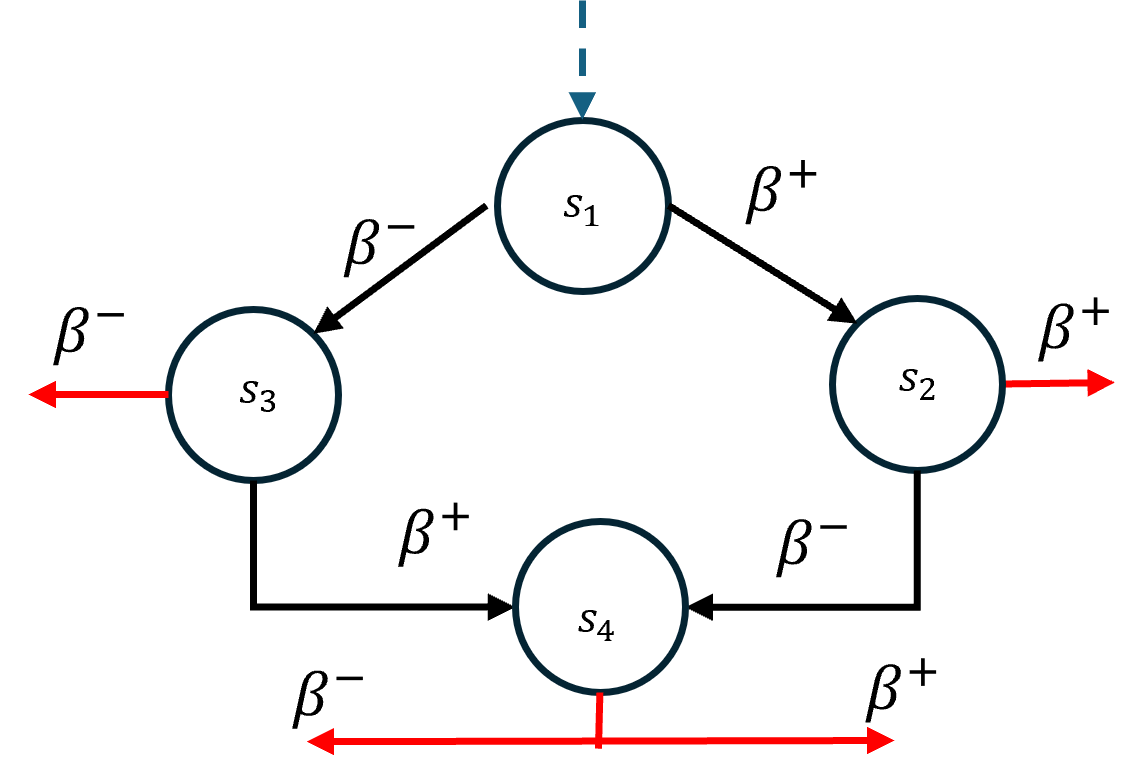
Figure 8: A hidden Markov representation of a cell in a semi-Markov CTRW. The particle exit is modeled in three Markov stages starting from $s_{1}$ and moving down to $s_{4}$. The red arrows indicate outputs from the cell. The dotted arrow indicates input from the previous cell. In the periodic case, the cell output is looped back into the initial state $s_{1}$.

The system lattice can now be visualized as a ring of such cells. A similar cell structure was used in [86].

A particle exits a lattice cell via a three-stage Markov process starting in state $s_{1}$. In the first stage, a move to either $s_{2}$ or $s_{3}$ is triggered by competing exponential distributions with rates $\beta^{+}$ and $\beta^{-}$ respectively. In the second stage, the particle immediately exits the cell if the distribution that triggered the transition in the first stage wins again. Otherwise, the particle moves to state $s_{4}$. In the third stage, a forward or backward exit occurs from state $s_{4}$, with rates $\beta^{+}$ and $\beta^{-}$ respectively. After the exit, depending on whether a forward or backward jump occurs, the particle then enters state $s_{1}$ of the next or preceding cell in the ring. For a three-site case, the dynamics is then given by a $12\times 12$ generator matrix. However, it is possible to reduce the matrix, since we are only interested in the statistics of the system current. As the transition probabilities are independent of the position on the ring, the current dynamics is homogeneous with respect to the cells. We may assume all exits from a cell loop back to state $s_{1}$ of the same cell and consider a simple $4\times 4$ Markov generator matrix

$$G=\begin{bmatrix}-\beta^{+}-\beta^{-}&\beta^{+}&\beta^{-}&0\\ \beta^{+}&-\beta^{+}-\beta^{-}&0&\beta^{-}\\ \beta^{-}&0&-\beta^{+}-\beta^{-}&\beta^{+}\\ \beta^{+}+\beta^{-}&0&0&-\beta^{+}-\beta^{-}\end{bmatrix}.$$ (56)

We obtain the SCGF for the current fluctuations of the above hidden Markov process following the standard procedure given for example in [3]. Weighting forward and backward transitions out of the cell (shown with red arrows in figure 8) with the exponential factors $e^{s}$ and $e^{-s}$, gives the tilted generator matrix

$$\tilde{G}(s)=\begin{bmatrix}-\beta^{+}-\beta^{-}&\beta^{+}&\beta^{-}&0\\ \beta^{+}e^{s}&-\beta^{+}-\beta^{-}&0&\beta^{-}\\ \beta^{-}e^{-s}&0&-\beta^{+}-\beta^{-}&\beta^{+}\\ \beta^{+}e^{s}+\beta^{-}e^{-s}&0&0&-\beta^{+}-\beta^{-}\end{bmatrix}.$$ (57)

Finally, the principal eigenvalue of the above generator matrix gives the required SCGF. We obtain this numerically for comparison against the reinforcement learning results in the main text.

A.3 Memory-induced ratchets

Semi-analytical results for current fluctuations in the hypoexponential and hyperexponential ratchets of section 5.1 were calculated by following a procedure similar to the one shown in the previous section.

For the hypoexponential ratchet, a lattice site has an equivalent cell structure with Markov states as shown in figure 9(a). The hypoexponential waiting-time distribution of the forward phase of the ratchet is represented by the Markov transitions across the states $s_{1}$ and $s_{2}$ connected in series, occurring with constant rates $\alpha_{1}$ and $\alpha_{2}$. A transition to the state $s_{3}$ is possible at each of the sites with reorientation rate $r$. The backwards phase is Markovian, driven only by exponential waiting-time distributions, therefore no hidden state description is needed; the particle simply transitions out of $s_{3}$ either to the next state in the backward process with rate $\beta$ or to $s_{1}$ in the forward phase with rate $r$. The cell structure in figure 9(a) is repeated to generate the equivalent hidden-Markov lattice for the hypoexponential ratchet with periodic boundaries. In the three-site example shown in figure 2 in the main text, there are three cells each containing two states in the outer ring and one in the inner ring. Thus, the transition dynamics can be defined by a $9\times 9$ generator matrix; via exponential weighting, we finally obtain the tilted generator

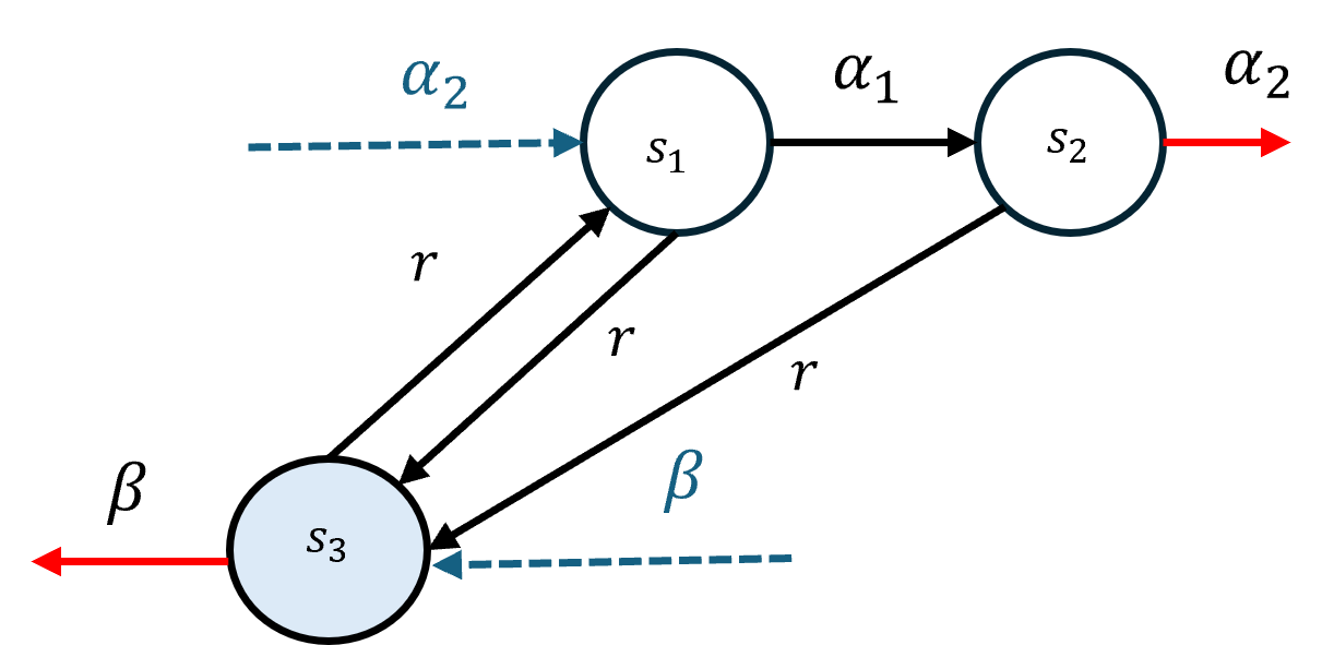
(a)

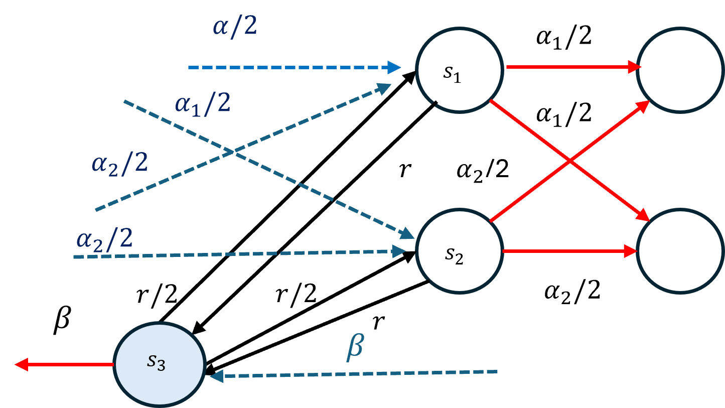
(b)

Figure 9: Hidden Markov cell structure for memory-dependent ratchets. (a) Hypoexponential ratchet. (b) Hyperexponential ratchet.

$$\tilde{G}(s)=$$

$$\begin{bmatrix}-\alpha_{1}-r&\alpha_{1}&0&0&0&0&r&0&0\\ 0&-\alpha_{2}-r&\alpha_{2}e^{s}&0&0&0&r&0&0\\ 0&0&-\alpha_{1}-r&\alpha_{1}&0&0&0&r&0\\ 0&0&0&-\alpha_{2}-r&\alpha_{2}e^{s}&0&0&r&0\\ 0&0&0&0&-\alpha_{1}-r&\alpha_{1}&0&0&r\\ \alpha_{2}&0&0&0&0&-\beta-r&0&0&r\\ r&0&0&0&0&0&-\beta-r&0&\beta e^{-s}\\ 0&0&r&0&0&0&\beta e^{-s}&-\beta-r&0\\ 0&0&0&0&r&0&0&\beta e^{-s}&-\beta-r\end{bmatrix}.$$ (58)

The hidden Markov cell structure for the hyperexponential ratchet is shown in figure 9(b). The forward phase now contains hidden states $s_{1}$ and $s_{2}$ connected in parallel over equiprobable branches. At each hidden state in the forward phase, the particle may choose to transition to $s_{3}$ in the backward phase, which again has purely Markovian transitions as in the case of the hypoexponential ratchet. After appropriately weighting the transitions in a three-site ring, we arrive at the tilted generator matrix

$$\tilde{G} (s)=$$

$$\begin{bmatrix}-\alpha_{1}-r&0&\frac{\alpha_{1}e^{s}}{2}&\frac{\alpha_{1}e^{s}}{2}&0&0&r&0&0\\ 0&-\alpha_{2}-r&\frac{\alpha_{2}e^{s}}{2}&\frac{\alpha_{2}e^{s}}{2}&0&0&r&0&0\\ 0&0&-\alpha_{1}-r&0&\frac{\alpha_{1}e^{s}}{2}&\frac{\alpha_{1}e^{s}}{2}&0&r&0\\ 0&0&0&-\alpha_{2}-r&\frac{\alpha_{2}e^{s}}{2}&\frac{\alpha_{2}e^{s}}{2}&0&r&0\\ \frac{\alpha_{1}e^{s}}{2}&\frac{\alpha_{1}e^{s}}{2}&0&0&-\alpha_{1}-r&0&0&0&r\\ \frac{\alpha_{2}e^{s}}{2}&\frac{\alpha_{2}e^{s}}{2}&0&0&0&-\alpha_{2}-r&0&0&r\\ r&0&0&0&0&0&-\beta-r&0&\beta e^{-s}\\ 0&0&r&0&0&0&\beta e^{-s}&-\beta-r&0\\ 0&0&0&0&r&0&0&\beta e^{-s}&-\beta-r\end{bmatrix}.$$ (59)

We obtain the SCGFs of the memory-induced ratchets by numerically calculating the principal eigenvalues of the tilted generators.

A.4 Gamma TASEP

In the two-site gamma TASEP of section 5.2.1, the scale parameter, $a=2$, was chosen for all gamma distributed waiting times. In the equivalent Markov representation, a hidden site is added (in series) for each gamma transition in the original lattice. Thus, the two-site gamma TASEP in section 5.2.1 is realized by the five-site hidden process shown in figure 10.

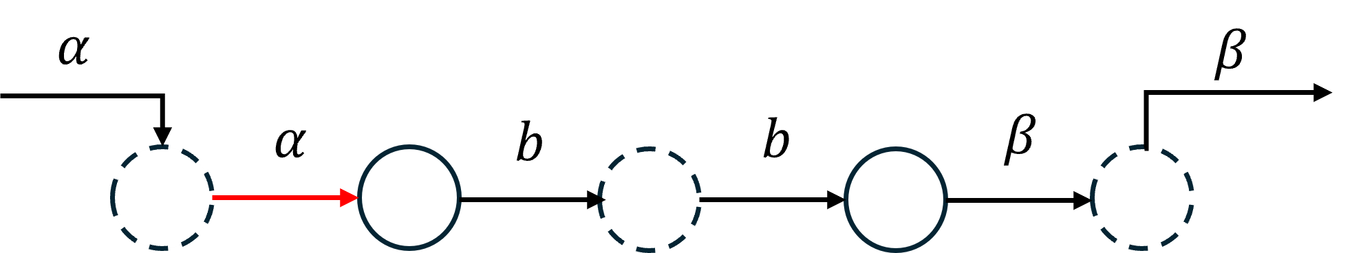
Figure 10: Equivalent hidden Markov model for the two-site gamma TASEP. The dotted circles represent the additional hidden sites, giving the fine-grained Markov representation of the coarse-grained gamma-distributed waiting times; $\gamma_{2,\alpha}(\tau)$ for arrivals, $\gamma_{2,b}(\tau)$ for bulk transitions and $\gamma_{2,\beta}(\tau)$ for the departures. The current fluctuations are measured across the red input arrow.

The dynamics must now satisfy a two-site exclusion condition, where a particle transition can occur only if two successive sites are unoccupied. This gives ten allowed configurations on the hidden lattice, with a $10\times 10$ Markov generator in the configuration space. Appropriately weighting this generator to count current into the system, gives the tilted matrix

$$\tilde{G}(s)=\begin{bmatrix}-\alpha&\alpha&0&0&0&0&0&0&0&0\\ 0&-\alpha&\alpha e^{s}&0&0&0&0&0&0&0\\ 0&0&-b&b&0&0&0&0&0&0\\ 0&0&0&-b&b&0&0&0&0&0\\ 0&0&0&0&-\alpha-\beta&\alpha&\beta&0&0&0\\ 0&0&0&0&0&-\alpha-\beta&0&\alpha e^{s}&\beta&0\\ \beta&0&0&0&0&0&-\alpha-\beta&\alpha&0&0\\ 0&\beta&0&0&0&0&0&-\alpha-\beta&0&\alpha e^{s}\\ 0&0&0&0&0&0&0&0&-\beta&\beta\\ \beta&0&0&0&0&0&0&0&0&-\beta\end{bmatrix}.$$ (60)

As in the previous examples, the SCGF is given by the principal eigenvalue of the tilted generator matrix.

Appendix B Recurrent neural networks for large systems

For systems with large state spaces, such as the TASEP model of section 5.2.2, the classic feed-forward (dense) neural networks of section 4.5 are replaced with recurrent neural networks (RNNs).

B.1 RNN Structure

The feed-forward neural network is a weighted connected graph, where each output of the previous layer is connected to the input of the current layer. Adding more layers to the network, or in other words increasing the network depth, increases the number of weighted connections, leading to performance drops due to difficulties in gradient computations. Another issue is that feed-forward neural networks, at the outset, do not include dependencies in the input sequence. We describe next how RNNs address these issues; they are especially useful in problems with sequential data and present a viable framework for processing systems with large state spaces.

The recurrent neural network, as the name suggests, has a looped structure which is shown in figure 11. Each instance or time step of the loop is now considered a layer of the network. This is visualized by the unfolded representation of the RNN on the right-hand side of figure 11. A large vector of sequential data is fed component-wise to each layer of the network. At each time step, the internal or hidden state of the RNN is updated according to the data received and then passed on to the next layer. The RNN thus propagates information across the layers to learn the sequential correlations in the data. The information flow is controlled by the weights of the RNN. Due to the looped structure, the same set of weights are shared among the layers, reducing the number of parameters to learn.

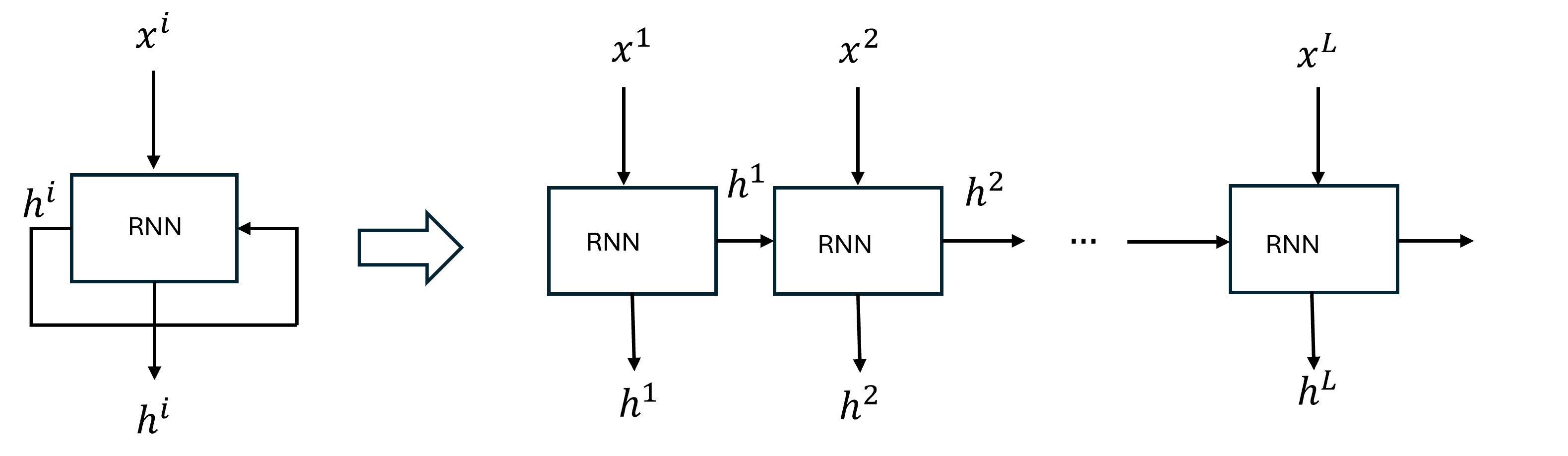
Figure 11: Recurrent neural unit. Left-hand side shows a recurrent cell with the corresponding unfolded network shown on the right-hand side.

In practice, popular variants of RNNs such as the so-called long short-term memory (LSTM) [87, 88] or the gated recurrent unit (GRU) [89, 90, 91] are favored over the basic RNN structure, as backpropagation causes the gradient to vanish when the number of layers in the basic RNN network becomes large. In section 5.2.2, we choose to use GRU units that include forgetting and that prioritize information from the most recent layers to update the current internal (hidden) state. Further details on the machinery of GRU may be found in [90]. We focus here on the implementation for processing large systems within the context of the reinforcement learning method presented in the main text.

B.2 GRUs for processing large systems with memory

In systems like the TASEP of section 5.2.2, obviously the state space grows with the increase in the number of sites, suggesting that a large inefficient feed-forward network with many layers is required for the neural reinforcement learning. However, since our TASEP states inherently have a sequential structure in the spatial dimension, such a large feed-forward network can be avoided by using a recursive neural network to increase the processing efficiency.

We use GRU-based networks to process the spatial sequence describing the present system state. The actor networks in figures 12 and 13 show how the recurrent architecture can be used to distill the combined information about the configuration and memory into transition policies. The figures show multiple GRUs (unfolded) in a stacked architecture, where the outputs of one GRU are fed as inputs to another GRU. For the many-site TASEP, two stacked GRUs were used. The GRU layers transform the information about the current state and memory to create an encoded (or embedded) vector, $\mathbf{E}=[E^{1},E^{2}...,E^{L}]$. The encoding $\mathbf{E}$ can now be used to generate polices with a shallow feed-forward network. A similar structure was used for the critic learning the value functions.

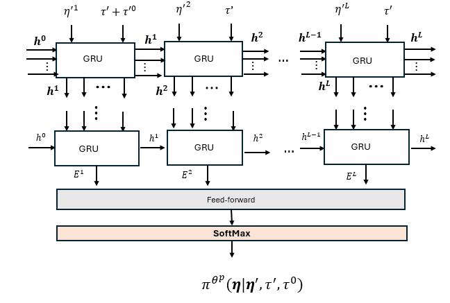
Figure 12: A GRU actor architecture for policy $\pi^{p}$. The GRUs systematically process the configuration, waiting time at the present configuration and the time since the arrival clock has been active, to form the encoding $\boldsymbol{E}=[E^{1},E^{2},...,E^{L}]$. A shallow feed-forward network transforms the encoding to the required transition.

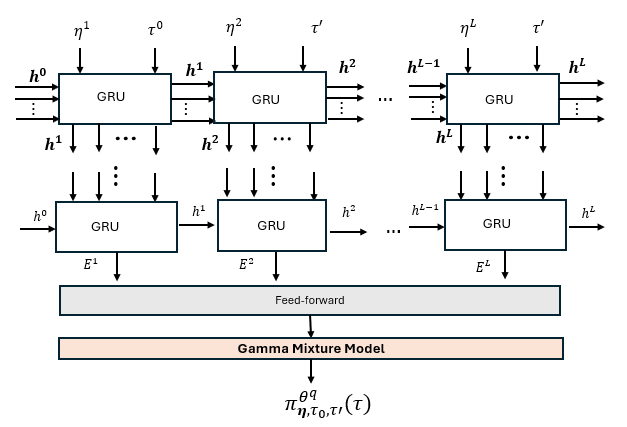
Figure 13: A GRU actor architecture for policy $\pi^{q}$. The GRUs systematically process the present configuration, the waiting time at the previous configuration and the time since the arrival clock has been active to give an encoding $\boldsymbol{E}=[E^{1},E^{2},...,E^{L}]$. The policy strictly does not need the waiting time $\tau^{\prime}$, but a marginal improvement was observed when it was included. Again, a shallow feed-forward network transforms the encoding to the required transition.

Appendix C Implementation details

The neural networks for all the examples were implemented using pytorch [92], a machine learning library for python. Learning rates $(\alpha_{{}_{\theta^{p}}},\alpha_{\theta^{q}},\alpha_{\theta^{v}})=(10^{-4},10^{-4},10^{-4})$ were chosen for the gradient update of the neural network weights in differential actor-critic of Algorithm 1. The learning rate to update the average reward was $\alpha_{r}=5\times 10^{-3}$.

As mentioned in the main text, the neural networks were trained on mini-batches. For the semi-Markov CTRW, memory-induced ratchets and two-site gamma TASEP examples, a batch size of $16$ was used. For the actors and the critic in these examples, we used feed-forward neural networks a maximum of three layers deep with $tanh$ activations, followed by a linear layer (without activation). The outputs of these networks were fed into layers performing the specialized operations explained in section 4.5. We found that this architecture was sufficient to accomplish the specific learning tasks. For the more complex many-site TASEP, two-stacked GRUs were used for the actors and the critic, followed by a single feed-forward layer with $tanh$ activations and a final linear layer with no activation. For the policies, specialized operations were performed to the outputs of this architecture to obtain the relevant probability distributions. The networks in this case were trained on a graphics processing unit.

The exclusion conditions in the TASEP models were implemented by masking the relevant outputs (corresponding to the restricted transitions) in the actor learning the policy $\pi^{\theta^{p}}$, as was done in [12], before computing the softmax. The masking ensures the softmax gives zero probabilities for the restricted transitions.

Note that keeping the general overview of the architecture explained in mind, one is free to choose the specific machine learning model parameters, such as number of layers, batch sizes and learning rates. There is much scope for optimization in terms of speed and accuracy, depending on the given nonequilibrium problem and the available hardware.

References

- [1] Derrida B 2007 J. Stat.Mech: Theory Exp. 2007 P07023
- [2] Touchette H 2009 Phys. Rep. 478 1–69
- [3] Touchette H 2012 A basic introduction to large deviations: Theory, applications, simulations (Preprint arXiv:1106.4146)
- [4] Ellis R S 1995 Scand. Actuarial J. 1995 97–142
- [5] Ellis R S 2006 Large Deviation Property and Asymptotics of Integrals (Berlin, Heidelberg: Springer Berlin Heidelberg) pp 30–58
- [6] Lecomte V and Tailleur J 2007 J. Stat. Mech: Theory Exp. 2007 P03004
- [7] Giardinà C, Kurchan J and Peliti L 2006 Phys. Rev. Lett. 96(12) 120603
- [8] Bolhuis P G, Chandler D W, Dellago C and Geissler P L 2002 Annu. Rev. Phys. Chem. 53 291–318
- [9] Asghar S, Pei Q X, Volpe G and Ni R 2024 Nat. Mach. Intell. 6 1370–1381
- [10] Rose D C, Mair J F and Garrahan J P 2021 New J. Phys. 23 013013
- [11] Das A, Rose D C, Garrahan J P and Limmer D T 2021 J. Chem. Phys 155 134105
- [12] Gillman E, Rose D C and Garrahan J P 2024 Phys. Rev. Lett. 132(19) 197301
- [13] Whitelam S, Jacobson D and Tamblyn I 2020 J. Chem. Phys 153 044113
- [14] Cavallaro M and Harris R J 2016 J. Phys. A: Math. Theor. 49 47LT02
- [15] Esposito M and Lindenberg K 2008 Phys. Rev. E 77(5) 051119
- [16] Shlesinger M 1974 J. Math. Phys. 10 421–434
- [17] Montroll E W and Weiss G H 2004 J. Math. Phys. 6 167–181
- [18] Chvosta P and Reineker P 1999 Physica A 268 103–120
- [19] Haus J and Kehr K 1987 Phys. Rep. 150 263–406
- [20] Andrieux D and Gaspard P 2008 J. Stat. Mech: Theory Exp. 11 P11007
- [21] Chari M K 1994 Oper. Res. Lett. 15 157–161
- [22] Gillespie D T 1976 J. Comput. Phys. 22 403–434
- [23] Anderson W J 2012 Continuous-time Markov chains: An applications-oriented approach (New York, NY: Springer)
- [24] Zia R K P and Schmittmann B 2006 J. Phys. A: Math. Gen. 39 L407
- [25] Zia R K P and Schmittmann B 2007 J. Stat. Mech: Theory Exp. 2007 P07012
- [26] Schütz G M and Trimper S 2004 Phys. Rev. E 70(4) 045101
- [27] Kenkre V M 2007 Analytic formulation, exact solutions, and generalizations of the elephant and the alzheimer random walks (Preprint arXiv:0708.0034)
- [28] Harris R J and Touchette H 2009 J. Phys. A: Math. Theor. 42 342001
- [29] Harris R J 2015 J. Stat. Mech: Theory Exp. 2015 P07021
- [30] Jack R L and Harris R J 2020 Phys. Rev. E 102(1) 012154
- [31] Harris R J and Touchette H 2017 J. Phys. A: Math. Theor. 50 10LT01
- [32] Harris R J, Rákos A and Schütz G M 2005 J. Stat. Mech: Theory Exp. 2005 P08003
- [33] Chetrite R and Touchette H 2015 J. Stat. Mech: Theory Exp. 2015 P12001
- [34] Jacobson D and Whitelam S 2019 Phys. Rev. E 100(5) 052139
- [35] Sutton R S and Barto A G 2018 Reinforcement Learning: An Introduction 2nd ed (Cambridge, MA: MIT Press)
- [36] Bertsekas D 1995 Dynamic Programming and Optimal Control vol 1 (Athena Scientific)
- [37] Mnih V, Kavukcuoglu K, Silver D, Rusu A A, Veness J, Bellemare M G, Graves A, Riedmiller M, Fidjeland A K, Ostrovski G, Petersen S, Beattie C, Sadik A, Antonoglou I, King H, Kumaran D, Wierstra D, Legg S and Hassabis D 2015 Nature 518 529–533
- [38] Mnih V, Badia A P, Mirza M, Graves A, Lillicrap T, Harley T, Silver D and Kavukcuoglu K 2016 Asynchronous methods for deep reinforcement learning Proceedings of The 33rd International Conference on Machine Learning (Proceedings of Machine Learning Research vol 48) ed Balcan M F and Weinberger K Q (New York, New York, USA: PMLR) pp 1928–1937
- [39] Schulman J, Wolski F, Dhariwal P, Radford A and Klimov O 2017 Proximal policy optimization algorithms (Preprint arXiv:1707.06347)
- [40] Haarnoja T, Zhou A, Hartikainen K, Tucker G, Ha S, Tan J, Kumar V, Zhu H, Gupta A, Abbeel P and Levine S 2019 Soft actor-critic algorithms and applications (Preprint arXiv:1812.05905)
- [41] Todorov E 2006 Linearly-solvable Markov decision problems Advances in Neural Information Processing Systems vol 19 ed Schölkopf B, Platt J and Hoffman T (MIT Press)
- [42] Sutton R S, Precup D and Singh S 1999 Artif. Intell. 112 181–211
- [43] Doshi B T 1979 J. Appl. Probab. 16 618–630
- [44] Schmidhuber J 1990 Reinforcement learning in Markovian and non-Markovian environments Advances in Neural Information Processing Systems vol 3 ed Lippmann R, Moody J and Touretzky D (Morgan-Kaufmann)
- [45] Farajtabar M, Azizan N, Mott A and Li A 2020 Orthogonal gradient descent for continual learning Proceedings of the Twenty Third International Conference on Artificial Intelligence and Statistics (Proceedings of Machine Learning Research vol 108) ed Chiappa S and Calandra R (PMLR) pp 3762–3773
- [46] Sutton R S, McAllester D, Singh S and Mansour Y 1999 Policy gradient methods for reinforcement learning with function approximation Advances in Neural Information Processing Systems vol 12 ed Solla S, Leen T and Müller K (MIT Press)
- [47] Konda V and Tsitsiklis J 1999 Actor-critic algorithms Advances in Neural Information Processing Systems vol 12 ed Solla S, Leen T and Müller K (MIT Press)
- [48] Bertsekas D 2020 Results Control Optim. 1 100003
- [49] Sutton R S 1988 Mach. Learn. 3 9–44
- [50] Mahadevan S 1996 Mach. Learn. 22 159–195
- [51] Silver D, Huang A, Maddison C J, Guez A, Sifre L, van den Driessche G, Schrittwieser J, Antonoglou I, Panneershelvam V, Lanctot M, Dieleman S, Grewe D, Nham J, Kalchbrenner N, Sutskever I, Lillicrap T, Leach M, Kavukcuoglu K, Graepel T and Hassabis D 2016 Nature 529 484–489
- [52] Hornik K, Stinchcombe M and White H 1989 Neural Networks 2 359–366
- [53] Goodfellow I J, Bengio Y and Courville A 2016 Deep Learning (Cambridge, MA: MIT Press)
- [54] Bishop C 1994 Mixture density networks Working paper Aston University URL https://api.semanticscholar.org/CorpusID:118227751
- [55] Magdon-Ismail M and Atiya A 1998 Neural networks for density estimation Advances in Neural Information Processing Systems vol 11 ed Kearns M, Solla S and Cohn D (MIT Press)
- [56] Chen S X 2000 Ann. Inst. Stat. Math. 52 471–480
- [57] Wiper M, Insua D R and Ruggeri F 2001 J. Comput. Graphical Stat. 10 440–454
- [58] Papamakarios G, Nalisnick E, Rezende D J, Mohamed S and Lakshminarayanan B 2021 J. Mach. Learn. Res. 22 1–64
- [59] Rezende D J and Mohamed S 2015 Variational inference with normalizing flows Proceedings of the 32nd International Conference on International Conference on Machine Learning - Volume 37 ICML’15 (JMLR.org) p 1530–1538
- [60] Zeng Y 2019 Context aware machine learning (Preprint arXiv:1901.03415)
- [61] Niu Z, Zhong G and Yu H 2021 Neurocomputing 452 48–62
- [62] Vaswani A, Shazeer N, Parmar N, Uszkoreit J, Jones L, Gomez A N, Kaiser L u and Polosukhin I 2017 Attention is all you need Advances in Neural Information Processing Systems vol 30 ed Guyon I, Luxburg U V, Bengio S, Wallach H, Fergus R, Vishwanathan S and Garnett R (Curran Associates, Inc.)
- [63] Kingma D P and Ba J 2017 Adam: A method for stochastic optimization (Preprint arXiv:1412.6980)
- [64] French R M 1999 Trends Cognit. Sci. 3 128–135
- [65] Wang Z, Bapst V, Heess N, Mnih V, Munos R, Kavukcuoglu K and de Freitas N 2017 Sample efficient actor-critic with experience replay (Preprint arXiv:1611.01224)
- [66] Cox D R 1955 Mathematical Proceedings of the Cambridge Philosophical Society 51 313–319
- [67] Aalen O 2005 Scand. J. Stat. 22 447–463
- [68] Feynman R P L R B and M S 1996 Feynman Lectures on Physics (Addison Wesley, Reading, Mass.)
- [69] Cubero D, Lebedev V and Renzoni F 2010 Phys. Rev. E 82(4) 041116
- [70] Reimann P 2000 Phys. Rep. 361 57–265
- [71] Magnasco M O 1993 Phys. Rev. Lett. 71(10) 1477–1481
- [72] Ethier S N and Lee J 2017 R. Soc. Open Sci. 5 171685
- [73] Roberts C and Zhen Z 2023 Phys. Rev. E 108(1) 014139
- [74] Angelani L, Costanzo A and Leonardo R D 2011 Europhys. Lett. 96 68002
- [75] Spitzer F 1970 Adv. Math. 5 246–290
- [76] Lazarescu A 2015 J. Phys. A: Math. Theor. 48 503001
- [77] Gorissen M and Vanderzande C 2012 J. Stat. Phys. 148 628–636
- [78] Bellman R 1957 Dynamic Programming Rand Corporation research study (Princeton University Press)
- [79] Krizhevsky A, Sutskever I and Hinton G E 2012 Imagenet classification with deep convolutional neural networks Advances in Neural Information Processing Systems vol 25 ed Pereira F, Burges C, Bottou L and Weinberger K (Curran Associates, Inc.)
- [80] van den Oord A, Dieleman S, Zen H, Simonyan K, Vinyals O, Graves A, Kalchbrenner N, Senior A W and Kavukcuoglu K 2016 Wavenet: A generative model for raw audio Speech Synthesis Workshop
- [81] Devlin J, Chang M W, Lee K and Toutanova K 2019 Bert: Pre-training of deep bidirectional transformers for language understanding North American Chapter of the Association for Computational Linguistics
- [82] Bañuls M C and Garrahan J P 2019 Phys. Rev. Lett. 123(20) 200601
- [83] Metz F and Bukov M 2023 Nature Machine Intelligence 5 780–791
- [84] Gorissen M, Hooyberghs J and Vanderzande C 2009 Phys. Rev. E 79 020101
- [85] Garrahan J P, Jack R L, Lecomte V, Pitard E, van Duijvendijk K and van Wijland F 2009 J. Phys. A: Math. Theor. 42 075007
- [86] Maes C, Netočný K and Wynants B 2009 J. Phys. A: Math. Theor. 42 365002
- [87] Hochreiter S and Schmidhuber J 1997 Neural Comput. 9 1735–80
- [88] Van Houdt G, Mosquera C and Nápoles G 2020 Artif. Intell. Rev. 53 5929–5955
- [89] Cho K, van Merrienboer B, Gulcehre C, Bahdanau D, Bougares F, Schwenk H and Bengio Y 2014 Learning phrase representations using RNN encoder-decoder for statistical machine translation (Preprint arXiv:1406.1078)
- [90] Chung J, Gulcehre C, Cho K and Bengio Y 2014 Empirical evaluation of gated recurrent neural networks on sequence modeling (Preprint arXiv:1412.3555)
- [91] Mohsen S 2023 Multimedia Tools Appl. 82 47733–47749
- [92] Paszke A, Gross S, Massa F, Lerer A, Bradbury J, Chanan G, Killeen T, Lin Z, Gimelshein N, Antiga L, Desmaison A, Köpf A, Yang E, DeVito Z, Raison M, Tejani A, Chilamkurthy S, Steiner B, Fang L, Bai J and Chintala S 2019 Pytorch: An imperative style, high-performance deep learning library (Preprint arXiv:1912.01703)