Decoherence of Schrödinger cat states in light of wave/particle duality

Abstract

We challenge the standard picture of decohering Schrödinger cat states as an ensemble average obeying a Lindblad master equation, brought about locally from an irreversible interaction with an environment. We generate self-consistent collections of pure system states correlated with specific environmental records, corresponding to the function of the wave-particle correlator first introduced in Carmichael et al. [Phys. Rev. Lett. 85, 1855 (2000)]. In the spirit of Carmichael et al. [Coherent States: Past, Present and Future, pp. 75–91, World Scientific (1994)], we find that the complementary unravelings evince a pronounced disparity when the “position” and “momentum” of the damped cavity mode—an explicitly open quantum system—are measured. Intensity-field correlations may largely deviate from a monotonic decay, while Wigner functions of the cavity state display contrasting manifestations of quantum interference when conditioned on photon counts sampling a continuous photocurrent. In turn, the conditional photodetection events mark the contextual diffusion of both the net charge generated at the homodyne detector, and the electromagnetic field amplitude in the resonator.

Coherent states occupy a central position in quantum electrodynamics (QED). They create a connection between quantum and semiclassical theories of photoelectric detection Mandel (1958); Kelley and Kleiner (1964); Davidson and Mandel (1968); Kimble et al. (1977); Saleh (1978); Srinivas and Davies (1981); Mandel (1981); Srinivas and Davies (1982); Car (1993a): being eigenstates of an operator that annihilates photons from the electromagnetic field, they are natural candidates of quantum states of light that have the same effect on a photoelectric detector as coherent fields. Coherent states are also essential in telling apart classical and non-classical optical fields, featuring in the definition of the Glauber–Sudarshan $P$-representation Sudarshan (1963); Glauber (1963a) which sets the boundary. In fact, Glauber established their central place in his early work on quantum theory of coherence, which revolved around an analysis of photoelectric detection Glauber (1963b, c, a). With the advent of cavity and circuit QED, non-classical states of light were routinely within experimental reach and control in configurations where one atom, be it natural or artificial strongly interacts with one or a few photons. In situations of the like, the $P$-representation no longer maps quantum dynamics into a classical stochastic process, while proposed modifications to press on with such a mapping come with their own shortcomings Carmichael (2008).

Keeping the master equation (ME) description of a single decaying cavity mode as an open QED system explicitly in mind Davies (1976); Gerry and Knight (1997); Breuer and Petruccione (2007); Carmichael (2013); Minganti et al. (2016); Mamaev et al. (2018); Lebreuilly et al. (2019); Zhou et al. (2021); Zapletal et al. (2022); Krauss et al. (2023); Kozin et al. (2024), the formalism of quantum trajectories starts with photoelectric detection and addresses the following question: How does the evolution of the quantum oscillator state run in parallel with the classical stochastic process of photoelectric counts? The answer is given by a quantum mechanical theory which is able to simulate the evolution of the oscillator before taking the ensemble average to form the reduced system density operator $\rho(t)$. In this process, a quantum and a classical stochastic process are consistently coupled. Here we will make use of this coupling to investigate the decay of macroscopic superposition states Walls and Milburn (1985); Phoenix (1990); Kim and Bužek (1992); Brune et al. (1992); Zurek (2003a); Romero-Isart et al. (2010); Carmichael (2013); Girvin (2019); Dakić and Radonjić (2017); Qin et al. (2021) in conditional homodyne detection Yurke and Stoler (1987); Schleich et al. (1991); Carmichael et al. (2000, 2004); Carmichael and Nha (2004); Marquina-Cruz and Castro-Beltran (2008), an extension of the intensity correlation technique and its reliance on a conditional measurement, introduced by Hanbury-Brown and Twiss Brown and Twiss (1956); Brown et al. (1958, 1957). In 1986, Yurke and Stoller Yurke and Stoler (1986) proposed an idea on how a macroscopic superposition state might be prepared and subsequently observed by means of homodyne detection Wiseman and Milburn (1993); Car (1993b); Carmichael (2008); Wiseman and Milburn (2009). Several alternative schemes and physical systems have been suggested since Wolinsky and Carmichael (1988); Song et al. (1990); Brune et al. (1992); Monroe et al. (1996); Dakna et al. (1997); Agarwal et al. (1997); Gerry (1999); Lund et al. (2004); Jeong et al. (2005); Haroche and Raimond (2006); Glancy and de Vasconcelos (2008); Vlastakis et al. (2013); Haroche (2013); Leghtas et al. (2015); Bergmann and van Loock (2016); Michael et al. (2016); Ofek et al. (2016); Liao et al. (2016); Wang et al. (2016); Girvin (2019); Song et al. (2019); Omran et al. (2019); Joshi et al. (2021); Lewenstein et al. (2021); Rivera-Dean et al. (2021, 2022); Cosacchi et al. (2021); Pogorelov et al. (2021); Takase et al. (2021); Zhou et al. (2021); Wang et al. (2022); He et al. (2023); Ayyash et al. (2024); Bocini and Fagotti (2024); Kozin et al. (2024); Hotter et al. (2024); Yu et al. (2024); Torres et al. (2024), while later work also established that the photoelectron counting distribution in homodyne detection is given by a marginal of the Wigner function representing the state of the cavity—the local oscillator phase determines the marginal Vogel and Risken (1989); Smithey et al. (1993).

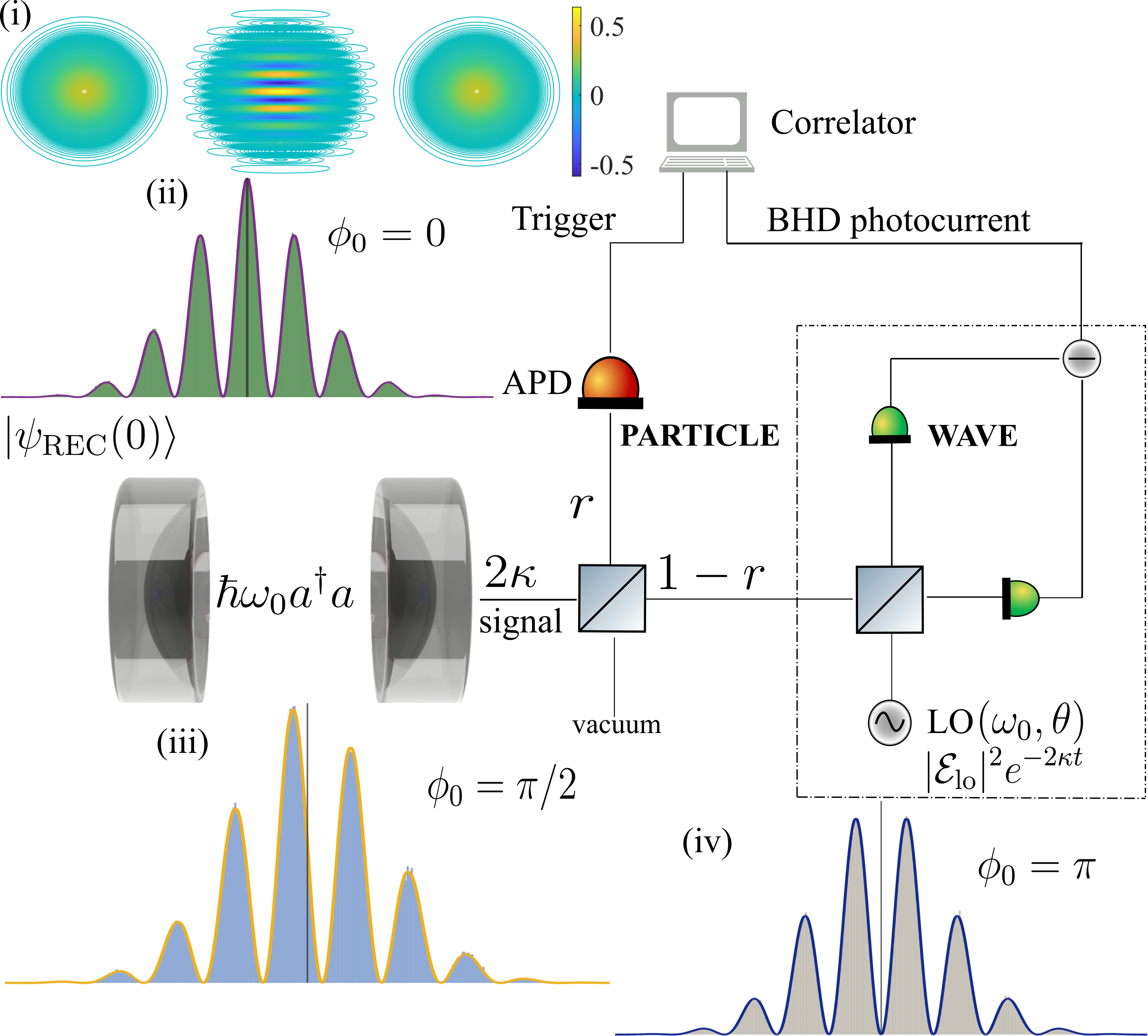
Figure 1: Schematic illustration of the wave-particle correlator (center) realizing conditional homodyne detection. The device operates with a fraction $r$ of the input light flux going to an avalanche photodiode (APD) in the “trigger” channel, and the remaining $1-r$ directed to a balanced mode-matched homodyne detector (BHD). The BHD samples the quadrature phase amplitude that is in phase with the local oscillator (LO) field; $\theta$ is the LO phase. The cavity mode $a$ is prepared in the superposition of coherent states (2) at time $t=0$, from which it decays to produce the scattered field (signal). Inset (i) depicts a contour plot of the Wigner function $W(x+iy;t=0)$ of the initial state (2), with $A=4$ and $\phi_{0}=0$. Insets (ii)–(iv) depict histograms of the cumulative charge $Q_{\theta=\pi/2}$ deposited on the BHD after the light has left the cavity, when the correlator operates with $r=0$ and $\theta=\pi/2$, for an initial Schrödinger cat state with $A=4$ and: $\phi_{0}=0$ (ii), $\pi/2$ (iii) and $\pi$ (iv). The vertical lines indicate the location of $Q_{\pi/2}=0$.

Data of the discrete, particle type, and continuous wave type are simultaneously collected Carmichael (2001), such that light scattered from a cavity initially prepared in a Schrödinger cat state Schrödinger (1935); Dodonov et al. (1974); Gerry and Knight (1997); Haroche and Raimond (2006); Neergaard-Nielsen et al. (2006); Ourjoumtsev et al. (2006, 2007); Sychev et al. (2017); Hacker et al. (2019); Pan et al. (2023) is seen in the simulated experiment to act as particle and wave. Both attributes serve to explain why $\rho(t)$ changes from a pure-state to a mixed-state density operator in a time much shorter than the cavity decay time by means of an unbalance in the two components of the superposition, operationally ascertained. Furthermore, they associate the quantum interference of a macroscopic Schrödinger cat, with the emission rate of cavity photons that condition its manifestation. Coupling superposition states to another subsystem readily tracks the operational consequences of quantum coherence. For instance, a joint measurement of a shifted parity operator Lutterbach and Davidovich (1997); Girvin (2019) and the projection of the Bloch vector of an atom entangled to the cat state leads to a correlation where the Wigner function of the cavity is weighted by the atomic spin orientations Wódkiewicz (2000). In a twist, detecting dipole radiation from the dressed states of Jaynes–Cummings interaction Car (1993c); Alsing and Carmichael (1991); Alsing et al. (1992); Solano et al. (2003) in a phase sensitive way via homodyne detection realizes an optical analogue of the Stern–Gerlach experiment Venugopalan et al. (1995); Venugopalan (1997) where the conditioned wavefunction makes a selection between initially superposed dressed states Carmichael et al. (1994). Conditional homodyne detection of a single system mode prepared in a coherent-state superposition resolves correlations similar to those read from entangled subsystems in various configurations Fortunato et al. (2000); Li et al. (2017); Mamaev et al. (2018); Lebreuilly et al. (2019); Giulio et al. (2019); Kfir (2019); Dahan et al. (2021); Cosacchi et al. (2021); Stammer et al. (2022); Wang et al. (2022); Zapletal et al. (2022); Pan et al. (2023); Torres et al. (2024). It does so by preserving or destroying the quantum coherence monitored through continuous measurement Davies (1976); Bergquist et al. (1986); Nagourney et al. (1986); Sauter et al. (1986); Cook (1988); Belavkin (1990); Barchielli and Belavkin (1991); Dalibard et al. (1992); Gardiner et al. (1992); Dum et al. (1992); Mølmer et al. (1993); Blanchard and Jadczyk (1995); Gisin and Percival (1997); Plenio and Knight (1998); Percival (1998); Mabuchi and Wiseman (1998); Peil and Gabrielse (1999); Brun (2002); Wiseman (2002); Gleyzes et al. (2007); Hegerfeldt (2009); Barchielli and Gregoratti (2012); Minganti et al. (2016); Minev et al. (2019).

We are concerned with a set of quantum-trajectory unravelings of the primordial Lindblad master equation Lindblad (1976) modelling the decay of a single cavity mode with frequency $\omega_{0}$ Carmichael (1999a); Breuer and Petruccione (2007):

$$\frac{d\rho}{dt}=\kappa(2a\rho a^{\dagger}-a^{\dagger}a\rho-\rho a^{\dagger}a),$$ (1)

written in the interaction picture with respect to the system Hamiltonian $H_{S}=\hbar\omega_{0}a^{\dagger}a$; here, $2\kappa$ is the photon loss rate. At $t=0$, the cavity mode $a$ is prepared in the macroscopic superposition state

$$|\psi_{\rm REC}(0)\rangle=\frac{|A\rangle+e^{i\phi_{0}}|-A\rangle}{\sqrt{2[1+\cos\phi_{0}\exp(-2A^{2})]}},$$ (2)

a Schrödinger cat state with a fixed phase difference between its two components. $A$ is any positive number, and $0\leq\phi_{0}<2\pi$.

The complementary unravelings Car (1993d); Carmichael (1999b); Wiseman and Gambetta (2012) are produced under the action of the wave-particle correlator Carmichael et al. (2000); Foster et al. (2000); Reiner et al. (2001); Carmichael et al. (2004) in the following fashion. Photons (particles) produce trigger “clicks” in an avalanche photodiode (APD) producing conditioned records of an electromagnetic field amplitude (wave) in the photocurrent output of a balanced homodyne detector (BHD) Yuen and Chan (1983). The BHD samples the quadrature phase amplitude with the local oscillator field phase $\theta$ (with $0\leq\theta<\pi$), defined as the operator $2\sqrt{2\kappa(1-r)}\,A_{\theta}$, where $A_{\theta}\equiv\frac{1}{2}(ae^{-i\theta}+a^{\dagger}e^{-i\theta})$ and $0\leq r\leq 1$. Meanwhile, the local-oscillator photon flux $|\mathcal{E}_{\rm lo}|^{2}e^{-2\kappa t}$ (with $\mathcal{E}_{\rm lo}|^{2}\gg A^{2}$) is matched to the decaying signal flux, to perform what is termed a mode matched conditional homodyne detection. The charge $dq_{\theta}$ deposited on the detector circuit in the interval from $t$ to $t+dt$ generates the BHD photocurrent $I_{\theta}(t)$ via $dI_{\theta}=-\tau_{d}^{-1}(I_{\theta}dt-dq_{\theta})$, where $\tau_{d}^{-1}$ is the detection bandwidth. Between triggers, the un-normalized conditioned state $|\overline{\psi}_{\rm REC}\rangle$ satisfies the following Stochastic Schrödinger Equation (SSE) Car (1993b); Reiner et al. (2001); Carmichael (2008):

$$d|\overline{\psi}_{\rm REC}\rangle=\left(-\kappa a^{\dagger}a\,dt+\sqrt{2\kappa(1-r)}\,a\,e^{-i\theta}d\xi\right)|\overline{\psi}_{\rm REC}\rangle,$$ (3)

where

$$d\xi \equiv e^{\kappa t}(Ge|\mathcal{E}_{\rm lo}|)^{-1}\,dq_{\theta}$$ (4)

$$=\sqrt{2\kappa(1-r)}[(e^{i\theta}\langle a^{\dagger}\rangle_{\rm REC}+e^{-i\theta}\langle a\rangle_{\rm REC})dt]+dW.$$

Here $e$ is the electronic charge and $G$ is the detector gain; $dW$ is a Gaussian-distributed random variable with zero mean and variance $dt$. The two averages in Eq. (4) are to be calculated with respect to the normalized conditioned state $|\psi_{\rm REC}(t)\rangle=|\overline{\psi}_{\rm REC}(t)\rangle/\sqrt{\langle\overline{\psi}_{\rm REC}(t)|\overline{\psi}_{\rm REC}(t)\rangle}$. The field measured at the APD is proportional to $\sqrt{2\kappa r}\,a$, while the sample making is triggered with a probability equal to $2\kappa r\langle\psi_{\rm REC}(t)|a^{\dagger}a|\psi_{\rm REC}(t)\rangle\,dt$. The cumulative charge deposited in the detector is defines as the real number

$$Q_{\theta}\equiv\sqrt{2\kappa}(Ge|\mathcal{E}_{\rm lo}|)^{-1}\int_{0}^{t}dq_{\theta}=\sqrt{2\kappa}\int_{0}^{t}e^{-\kappa t^{\prime}}d\xi^{\prime}.$$ (5)

By sampling an ongoing realization of the quadrature amplitude $A_{\theta}(t)$ for several “start” times $t_{j}$, $j=1,\ldots,N_{s}$, we can calculate an intensity-field correlation function Carmichael et al. (2000); Foster et al. (2000); Reiner et al. (2001); Denisov et al. (2002); Wiseman (2002); Carmichael et al. (2004) as the following conditioned average Car (1993b); Carmichael (2008),

$$h_{\theta}(\tau)\equiv(1/N_{s})2\sqrt{2\kappa(1-r)}\,\sum_{j=1}^{N_{s}}\langle A_{\theta}(t_{j}+\tau)\rangle_{\rm REC},$$ (6)

where $\langle A_{\theta}(t_{j}+\tau)\rangle_{\rm REC}=\langle\psi_{\rm REC}(t_{j}+\tau)|A_{\theta}|\psi_{\rm REC}(t_{j}+\tau)\rangle$. The sum over $j$ in Eq. (6) is evaluated as an average over past and future measurement records, before and after $t_{j}$ Carmichael (1997). The definition differs from the average photocurrent defined in Carmichael et al. (2000); Foster et al. (2000); Reiner et al. (2001) because the number of samples (starts) available along a single trajectory is limited by $N_{s}=A^{2}$, which is not sufficient to reduce the shot noise appreciably when $A^{2}$ is of the same order as the detection bandwidth (in units of the cavity bandwidth). For large-amplitude cats, we define $h_{\theta}(\tau)=(1/N_{s})\sum_{j=1}^{N_{s}}I_{\theta}(t_{j}+\tau)$, since there are enough samples to recover the signal out of the shot noise. We expect on average $N_{s}=rA^{2}$ trigger “clicks” along any trajectory. Note that the ME (1) predicts $\langle A_{\theta}(t)\rangle\sim 2\sin\phi_{0}\sin\theta\exp(-2A^{2})$ as an ensemble average for the initial state (2), which entails a vanishingly small $\langle h_{\theta}(\tau)\rangle$ for large initial photon numbers.

We start by setting $r=0$ to produce an uninterrupted continuous photocurrent at the BHD. In Fig. 1, we explore the effect of a varying phase between the two components in the initial superposition (2) to the cumulative charge released by the detector in the course of the entire evolution to the vacuum, for $\theta=\pi/2$. The Wigner function of the initial cavity state is Bužek et al. (1992); Carmichael et al. (1994); Wódkiewicz (2000); Schleich (2001a, b); Haroche and Raimond (2006)

$$W(x,y;t=0)=(2\pi e^{-A^{2}}\cosh A^{2})^{-1}e^{-2y^{2}}$$ (7)

$$\times[e^{-2(x-A)^{2}}+e^{-2(x+A)^{2}}+2e^{-2x^{2}}\cos(\phi_{0}+4Ay)],$$

where the last term (cosine) indicates quantum interference Zurek (2001). A contour plot of $W(x,y;t=0)$ for $\phi_{0}=0$ is given in inset (i). The Wigner function of the cavity state maintains the form of Eq. (7) with $A\to A(t)\equiv Ae^{-\kappa t}$ throughout the evolution dictated by ME (1) but, crucially, the cosine term is scaled by the factor $\exp[-2A^{2}(1-e^{-2\kappa t})]$: the greater the initial distance of the two components the faster the off-diagonal elements of $\rho(t)$ are dephased Walls and Milburn (1985); Phoenix (1990); Zurek (2003a, b). The disparity between the weights of the Gaussian peaks and the interference fringes brings in the short timescale $(2\kappa A^{2})^{-1}$ as the relevant decoherence time. Simultaneously, the Wigner function maintains its symmetry with respect to the $x$ and $y$ axis in all stages of the decay, and so do its corresponding marginals.

Setting $\theta=\pi/2$, the marginal distribution—obtained by integrating $W_{\rm REC}(x,y;t=0)$ along the $x$ axis—reads

$$P(y;t=0)=(\sqrt{2\pi}\cosh A^{2})^{-1}e^{-2y^{2}+A^{2}}[1+\cos(\phi_{0}+4Ay)].$$ (8)

The charge distribution $P(Q_{\pi/2})$ depicted in insets (ii-iv) and obtained after the light has left the cavity, in the decay of an ensemble of scattering records to the vacuum, and the marginal (8) are related by a simple scale factor with $Q_{\pi/2}=2y$. For all values of $\phi_{0}$ different to $0$ and $\pi$, $P(Q_{\pi/2})$ is asymmetric with respect to the $Q_{\pi/2}=0$ axis, but the average deposited cumulative charge remains zero, as expected from the vanishing integral $\int_{-\infty}^{\infty}yP(y;t=0)dy$. The probability of depositing $Q_{\pi/2}$ in the vicinity of zero scales as $2\cos^{2}(\phi_{0}/2)$, a direct indication of the initial phase. Therefore, mode-matched balanced homodyne detection performs a phase-sensitive tomogram Smithey et al. (1993); Lutterbach and Davidovich (1997); Welsch et al. (1999); Schleich (2001c); Vogel and Welsch (2006); Haroche and Raimond (2006) of the initial cavity state. In contrast, as we have previously noted, the interference term in the Wigner function corresponding to $\rho(t)$ for the initial state (2), disappears fast after the lapse of the decoherence time $(2\kappa A^{2})^{-1}$ and, together with it, any remain of the initial phase difference.

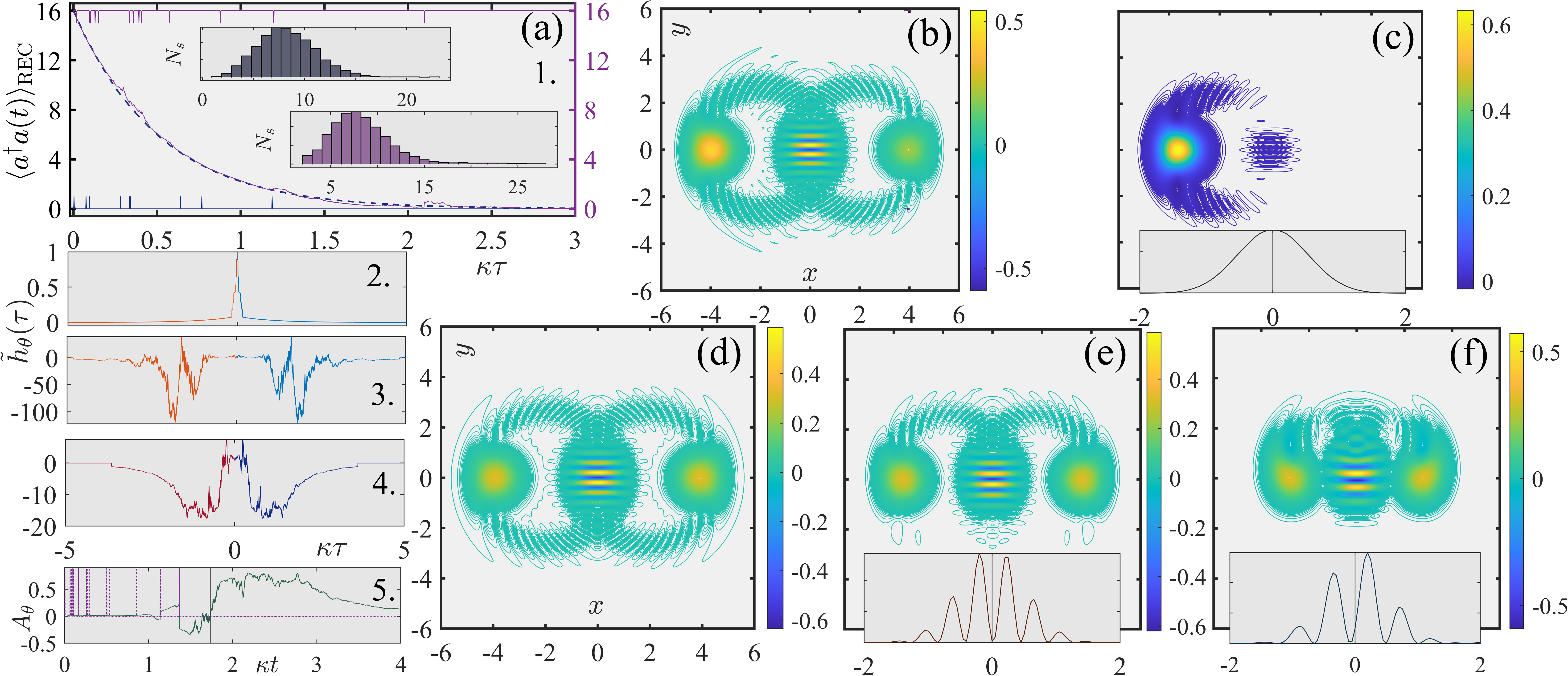
Figure 2: Conditioned Monte Carlo averages and state representations in single realizations. (a) 1: Conditioned intracavity photon number $\langle a^{\dagger}a(t)\rangle_{\rm REC}$ against three cavity lifetimes, for $\theta=0$ (dashed line) and $\pi/2$ (solid line). The strokes underneath ($\theta=0$) and above ($\theta=\pi/2$) the main plots indicate photon emissions triggering the homodyne current generation at the BHD. The two insets depict histograms of photon “click” resets $N_{s}$ for $\theta=0$ (top) and $\theta=\pi/2$ (bottom), over 4,000 realizations. (a) 2 – 4: Individual realizations of the intensity-field correlation function over its zero-delay value, $\tilde{h}_{\theta}(\tau)\equiv h_{\theta}(\tau)/h_{\theta}(0)$, for $\theta=0$ in (2), $\pi/2$ in (3) and $(\pi/2-\theta)=0.0078$ in (4). Frame (a5) depicts the conditioned average of the quadrature amplitude $A_{\theta}\equiv\langle A_{\theta}(t)\rangle_{\rm REC}$ corresponding to the trajectory of (a4). The dotted strokes in (a5) mark photon triggers, while the long vertical line in marks the time $\kappa t_{m}=(1/2)\ln(2A^{2})\approx 1.733$. (b) Contour plot of the conditioned Wigner function $W_{\rm REC}(x+iy;t_{1})$, at the time $\kappa t_{1}=0.004$ of the first photon trigger, along the trajectory of (a) generated for $\theta=0$; (c) Similar to (b), with $W_{\rm REC}(x+iy;t_{2})$ at the time $\kappa t_{2}=0.096$ of the third photon trigger. The lower inset depicts a numerical approximation of the conditioned marginal distribution $P_{\rm REC}(y;t_{2})=\int_{-\infty}^{\infty}W_{\rm REC}(x+iy;t_{2})\,dx$. (d) Contour plot of the conditioned Wigner function $W_{\rm REC}(x+iy;t_{1}^{\prime})$, at the time $\kappa t_{1}^{\prime}=0.018$ of the first photon trigger, along the trajectory of (a) generated for $\theta=\pi/2$; (e) Similar to (d), with $W_{\rm REC}(x+iy;t_{2}^{\prime})$, at the time $\kappa t_{2}^{\prime}=0.098$ of the second photon trigger; (f) Similar to (d), with $W_{\rm REC}(x+iy;t_{3}^{\prime})$, at the time $\kappa t_{3}^{\prime}=0.392$ of the eighth photon trigger along the trajectory generated for $\theta=\pi/2$. The lower insets in (e, f) depict numerical approximations of the conditioned marginal distributions $P_{\rm REC}(y;t_{k}^{\prime})=\int_{-\infty}^{\infty}W_{\rm REC}(x+iy;t_{k}^{\prime})\,dx$ for $k=2,3$, respectively. In all realizations, the initial state (2) has $A=4$ and $\phi_{0}=0$, while the correlator operates with $r=0.5$. The time step size is $\kappa\Delta t=0.002$, and the Fock-state basis is truncated at the $30$-photon level SM .

Let us now meet further evidence on how individual Monte Carlo realizations Car (1993a); SM under the action of the wave-particle correlator subvert the picture offered by the ME (1) and the Wigner function of the cavity state (7) formulated as a statistical mixture over an ensemble of pure states. Figure 2 depicts results obtained when the correlator operates with $r=0.5$. The pair of sample trajectories in frame (a1) show a decaying conditioned intracavity photon number $\langle a^{\dagger}a(t)\rangle_{\rm REC}$ for the same input state and two different settings of the LO phase, $\theta=0$ and $\theta=\pi/2$. No large differences are noted between the two records, perhaps apart from some collapses leading to higher conditioned photon emission probability deviating from the exponential decay in three instances. The trend of such ‘instability’ is visible in the histogram of $N_{s}$, which displays a longer tail when $\theta$ is set to $\pi/2$ and marks a clear departure from the Poisson distribution.

The time-symmetric intensity-field correlations plotted in frames (a2–a4) are the first quantities we meet that point to a clear operational disparity between two of the complementary unravelings. Since the average field ${\rm tr(\rho(t)A_{\theta})}$ [obtained from the solution of the ME (1)] is zero for $\theta=0$, we expect conditioned correlation functions with positive peaks to cancel those with negative over an ensemble of realizations. Sharply decaying intensity-field correlations for $\theta=0$ gradually transition to highly oscillatory functions with alternating sign and notable deviations from their zero-delay values as $\theta\to\pi/2$. For the latter setting, there is also a notable difference between the intensity-field functions obtained for different realizations, testifying to another manifestation [in addition to the one of Fig. 2(a1)] of the ‘instability’ reported in Carmichael (1999b). With every photon trigger, a phase change of $\pi$ is generated between the two components of the cat state. However, not all triggers lead to a phase change in the conditioned field amplitude. The last trigger is the one to direct the field quadrature to one of the periodic wells of the modulated potential governing the evolution of $Q_{\theta}$ Carmichael (1999b).

Pronounced deviations are routinely observed past the time $\kappa t_{m}\sim(1/2)\ln(2A^{2})\approx 1.733$ required for the potential to develop the periodic modulations SM . In Fig. 2(a3), for example, a large oscillation of the field amplitude occurs within a well dictating the oscillation frequency. The period and phase of this oscillation depend on the closeness of $\theta$ to $\pi/2$, as well as on the phase diffusion between the two components which determines whether a sign change occurs or not after an photon is recorded at the APD. In Figs. 2(a4–a5), we meet an intensity-field correlation and the corresponding realization of field amplitude, respectively, calculated for $14$ resets (well in excess of $rA^{2}=8$) when $\theta\to\pi/2$. At $\kappa t_{m}$, a large excursion of the field amplitude is initiated after the last photon trigger in the series. We note that a small deviation from $\theta=\pi/2$ produces a steady-state potential of rapidly decaying well heights with increasing $Q_{\theta}$ SM . The last reset resolves the accumulated diffusion and is responsible for a sign change in the field amplitude.

Wigner functions of the cavity state conditioned on photon triggers, calculated for the pure system state $\rho_{\rm REC}(t)=|\psi_{\rm REC}(t)\rangle\langle\psi_{\rm REC}(t)|$ SM , are as well at odds with the ensemble-averaged profile described by Eq. (7). We first measure the “position” of the oscillator ($\theta=0$) prepared in the superposition state (2). The contour plot depicted in Fig. 2(b) corresponds to the state collapse following a “click” occurring at a time which is an order of magnitude shorter than the decoherence time $(2\kappa A^{2})^{-1}$ predicted by the ME (1). The interference fringes are in place, although there is a visible asymmetry in the amplitude of the side Gaussian peaks. With the lapse of about three decoherence times, past the value $(2\kappa rA^{2})^{-1}$, the right peak has completely disappeared [Fig. 2(c)], leaving behind only insignificant trails of quantum interference. From that point onwards, the evolution essentially concerns the decay of a single coherent state with a peak centred at $-Ae^{-\kappa t}$. For other trajectories generated for $\theta=0$, the single peak in the phase-space profile is centred at $Ae^{-\kappa t}$. Therefore, the conditioned states produced for an unraveling with $\theta=0$ challenge the decoherence picture offered by the ME (1) through a fast-developing unbalance between the two state components. Past the decoherence time, the statistics of the photon resets—the vast majority of the recorded APD “clicks”—align with a decaying coherent state. An unbalance of similar kind is also met in the direct-photodetection unraveling of the ME (1), where the times of photoelectron counts bring into play a dynamical competition for an initial superposition state of different amplitudes (Carmichael et al., 1994; Carmichael, 2013).

Measuring the “momentum” of the harmonic oscillator ($\theta=\pi/2$) restores the interference in the conditioned Wigner distributions at all times [Fig. 2(d–f)], even when the cavity contains half of its initial photons [Fig. 2(f)]. Phase diffusion over an ensemble of such states is responsible for a nearly uniform quantum phase distribution past the very short decoherence time. Moreover, the previous asymmetry with respect to the $y$-axis, is now developing with respect to the $x$-axis and distorts the interference, a trait also reflected in the conditioned marginals $P_{\rm REC}(y)$. Photon triggers interrupt the otherwise continuous phase diffusion by injecting a $\pi$-phase difference between the two components of the cat state, as it leaves the cavity to partly exist in the output field. The interference fringes in Figs. 2(d–f) resolve the phase change. Having explored key differences in correlations both in the time domain and the phase-space representation, we may ask the question how is the conditioned cavity state fed back to the photon trigger “clicks” that condition it.

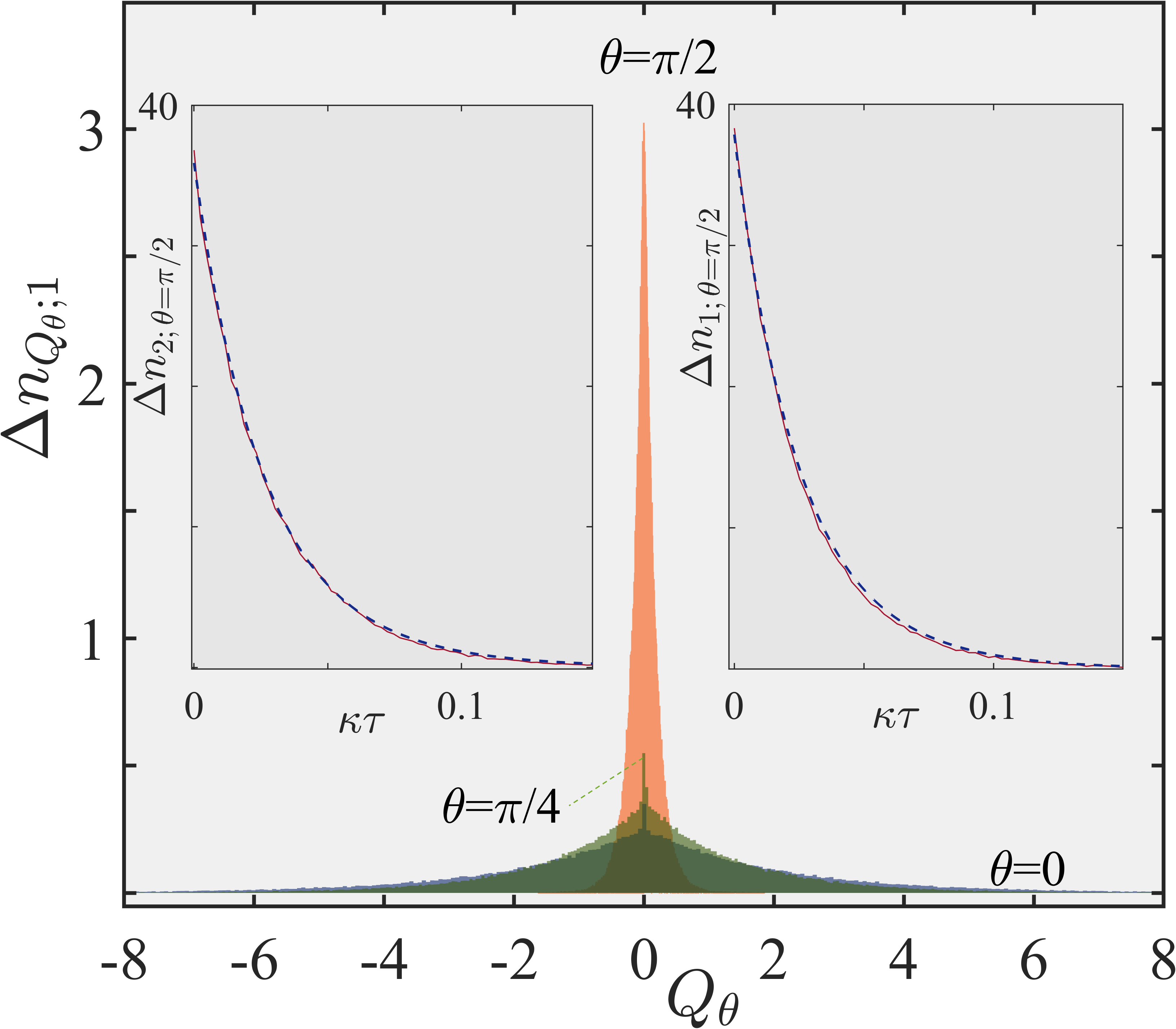
Figure 3: Distributions (histograms) of the net charge $Q_{\theta}$ deposited on the BHD at the time $t_{1}$ of the first photon trigger “click”, for three different settings of the LO phase, $\theta=0$, $\theta=\pi/4$ and $\pi/2$, indicated accordingly. The two insets either side of the histograms depict distributions of waiting times for the first (right) and second (left) photon emissions. $\Delta n_{1}$ ($\Delta n_{2}$) is the number of times photon 1 (photon 2) is emitted in the time interval $[\tau,\tau+\Delta\tau)$ Carmichael and Kim (2000). The continuous lines plot an ensemble average of 150,000 trajectories with bin size $\kappa\Delta\tau=0.0025$, while the dashed lines correspond to Eq. (10) with $A$ (right) and $A\to Ae^{-\kappa\tau_{\rm av}}$ (left). The initial state has: $A=20$, $\phi_{0}=\pi$, while the correlator operates with $r=0.05$.

Owing to the consistent coupling between a classical and a quantum stochastic process accomplished by quantum trajectory theory, we can derive analytical formulas connecting the charge production in the BHD and the trigger rate SM . As we have already seen, central to the evolution between the triggers is a diffusion either in the relative amplitude ($\theta=0$) or phase ($\theta=\pi/2$) [or a combination of the two for any other value of $\theta$] between the two components of the cat state (2), encapsulated in the null-measurement (no trigger “click”) record

$$|\overline{\psi}_{\rm REC,\,NULL}(t)\rangle=\exp[Q_{\theta}(t)A\sqrt{1-r}\,e^{-i\theta}]\,|Ae^{-\kappa t}\rangle+\exp[i\phi_{0}-Q_{\theta}(t)A\sqrt{1-r}\,e^{-i\theta}]\,|-Ae^{-\kappa t}\rangle.$$ (9)

At $t=0$, there is no net charge released from the detector ($Q_{\theta}=0$), whence we recover the un-normalized version of (2). At $\theta=\pi/2$, the exponents in (9) are purely imaginary, and the two components acquire a phase difference conditioned on the charge production at the BHD.

We focus on higher-amplitude cat states, such as those generated via conditional qubit-photon logic in circuit QED Vlastakis et al. (2013); Girvin (2019), to produce a large number of closely-spaced photon triggers. We operate the correlator with $r\ll 1$ to approach a pure balanced homodyne detection, yet satisfying $rA^{2}\gg 1$. The waiting-time distribution Carmichael et al. (1989); Carmichael and Kim (2000); Brandes (2008) for the first photon trigger, a characteristic particle-type attribute, is approximated by the analytical expression

$$w_{1}(\tau)\approx 2\kappa\frac{\exp[-rA^{2}(1-e^{-2\kappa\tau})]}{\int_{0}^{1}\exp[-rA^{2}(1-e^{-u})]du},$$ (10)

in line with a no-“click” measurement record obtained for a decaying coherent state with initial amplitude $\sqrt{rA^{2}}$ (Carmichael, 2013). The average time waited until the first photon emission is $\tau_{\rm av}=(2\kappa rA^{2})^{-1}$. The two insets of Fig. 3 show that the emission times of the first photon and the second, conditioned on the first reset, follow Eq. (10)—the latter with the replacement $A\to Ae^{-\kappa\tau_{\rm av}}$—when the “momentum” of the oscillator is measured. We find that the same trend is followed when measuring “position”; the obtained waiting-time distributions overlap with those shown in the figure. The cumulative charge diffusion conditioned on a photon detection and registered at the BHD, however, is very different in these two settings, as we can observe in the main plots of Fig. 3. Within the average photon emission time, the distribution of $Q_{\theta}$ diffuses at a similar rate when $\theta=0$ and $\theta=\pi/4$, while a pronounced and disproportionate difference is note for $\theta=\pi/2$. Considering that waves (quadrature amplitudes) condition the emission of particles (photons), we deduce from Eqs. (4), (5) that the conditioned electromagnetic field amplitude will vary at a slower rate when measuring “momentum”. For the latter setting, the charge distribution is found to remain virtually unchanged when conditioned on the second photon trigger as well.

In summary, our perspective has moved from inferring a set initial phase difference between the two components of a macroscopic quantum state superposition to measuring a dynamical and complementary amplitude and phase diffusion between them, in an unraveling method which takes both the particle and wave aspects of the scattered light into account. Notable differences in wave-particle correlations across complementary unravelings can be detected even for low-amplitude optical cat states subject to the current experimental limitations Neergaard-Nielsen et al. (2006); Ourjoumtsev et al. (2006, 2007); Takahashi et al. (2008); Huang et al. (2015); Ulanov et al. (2016); Sychev et al. (2017); Hacker et al. (2019); Takase et al. (2021); Li et al. (2024). The ‘tension’ between particles and waves Carmichael (2001) is revealed via two distinct timescales: in the one extreme, when the local oscillator is tuned to measure “position”, a strong unbalance between the two parts develops from the very start. By the lapse of the decoherence time required to turn the initial pure state into a statistical mixture in the ensemble average governed by the ME, the interference pattern effectively disappears while the cavity contains a significant amount of excitation. Most photons are subsequently emitted in the presence of a single coherent state in the cavity. On the other end, when the local oscillator is tuned to measure “momentum”, the interference fringes make their appearance late, after $\ln(2A^{2})$ photon decay times, when the cavity output pulse has reached the tail of the exponential decay. Occasional photon bursts occur as rare fluctuations in that timescale—the ones responsible for the long tail in the lower histogram of Fig. 2(a1). The timescale separation leaves no room for the quantum interference to influence the waiting-time distribution of the overwhelming majority of the emitted photons resetting the balanced homodyne detection. Nonetheless, photon emission times serve as diffusion markers of the charge generated at the homodyne detector, and the electromagnetic field amplitude in the cavity. Such markers are to be applied through conditioned cavity state tomograms Smithey et al. (1993); Lutterbach and Davidovich (1997); Nogues et al. (2000); Schleich (2001c); Deléglise et al. (2008); Hofheinz et al. (2008, 2009); Eichler et al. (2012); Haroche (2013); Blais et al. (2021); Ahmed et al. (2021a, b); Wang et al. (2022); He et al. (2023), and are embedded in a highly contextual intensity-field correlation function.

 

Supplementary Information

In the supplementary material, we detail the amplitude and phase diffusion of the conditioned state under the complementary wave-particle correlator unravelings. We derive a Fokker–Planck equation and an associated potential for mode-matched homodyne detection, and point to the link between the steady-state distribution and the marginal distribution of the initial Wigner function. We derive the general form of trajectories for conditional homodyne detection and, finally, delineate the steps to produce them via the corresponding Monte Carlo numerical procedure.

.1 Stochastic Schrödinger equation, Fokker–Planck equation and the associated potential in homodyne detection

.1.1 Stochastic Schrödinger equation and its transformation

We wish to determine the evolution of the cat state (2),

$$|\psi_{\rm REC}(0)\rangle=\frac{|A\rangle+e^{i\phi_{0}}|-A\rangle}{\sqrt{2[1+\cos\phi_{0}\exp(-2A^{2})]}},$$ (S.1)

conditioned upon the operation of the wave-particle correlator. Between photon triggers, corresponding to the action of the super-operator $2\kappa ra(|\overline{\psi}_{\rm REC}\rangle\langle\overline{\psi}_{\rm REC}|)a^{\dagger}$, the un-normalized conditioned state $|\overline{\psi}_{\rm REC}\rangle$ satisfies the following Stochastic Schrödinger Equation (SSE) Car (1993b); Reiner et al. (2001); Carmichael (2008):

$$d|\overline{\psi}_{\rm REC}\rangle=\left(-\kappa a^{\dagger}a\,dt+\sqrt{2\kappa(1-r)}\,a\,e^{-i\theta}d\xi\right)|\overline{\psi}_{\rm REC}\rangle,$$ (S.2)

where

$$d\xi\equiv e^{\kappa t}(Ge|\mathcal{E}_{\rm lo}|)^{-1}\,dq_{\theta}=\sqrt{2\kappa(1-r)}[(e^{i\theta}\langle a^{\dagger}\rangle_{\rm REC}+e^{-i\theta}\langle a\rangle_{\rm REC})dt]+dW.$$ (S.3)

In the above, $e$ is the electronic charge and $G$ is the detector gain; $dW$ is a Wiener increment with zero mean and variance $dt$. There equations govern the photocurrent production after taking into account the detection bandwidth.

To proceed we set Carmichael (2008)

$$|\overline{\psi}_{\rm REC}\rangle=e^{-\kappa a^{\dagger}a\,t}|\chi\rangle,$$ (S.4)

which transforms Eq. (S.2) to

$$d|\chi\rangle =\sqrt{2\kappa(1-r)}\,e^{\kappa a^{\dagger}at}\,a\,e^{-i\theta}e^{-\kappa a^{\dagger}at}\,d\xi|\chi\rangle$$ (S.5)

$$=\sqrt{2\kappa(1-r)}\,e^{-\kappa t}\,a\,e^{-i\theta}\,d\xi\,|\chi\rangle$$

$$=a\,\sqrt{1-r}\,dQ_{\theta}e^{-i\theta}|\chi\rangle,$$

with solution $|\chi\rangle=e^{a\,\sqrt{1-r}\,e^{-i\theta}Q_{\theta}}|\chi(0)\rangle=e^{a\,\sqrt{1-r}\,e^{-i\theta}Q_{\theta}}|\psi_{\rm REC}(0)\rangle$. Substituting for $|\psi_{\rm REC}(0)\rangle$ the initial state (2), we find

$$|\overline{\psi}_{\rm REC}(t)\rangle=\frac{\exp[-A^{2}(1-e^{-2\kappa t})]}{\sqrt{2[1+\cos\phi_{0}\exp(-2A^{2})]}}\left\{\exp[Q_{\theta}A\sqrt{1-r}\,e^{-i\theta}]\,|Ae^{-\kappa t}\rangle+\exp[i\phi_{0}-Q_{\theta}A\sqrt{1-r}\,e^{-i\theta}]\,|-Ae^{-\kappa t}\rangle\right\}.$$ (S.6)

The common prefactor is omitted in Eq. (9), while with $r=1$ we obtain the null-measurement record for direct photodetection Carmichael (2013).

Knowing the form of the system wavefunction in conditional homodyne detection, we can then evaluate the conditioned expectation of the quadrature amplitude until the first photon trigger:

$$\sqrt{1-r}\langle A_{\theta}(t)\rangle_{\rm REC} =\frac{1}{2}\sqrt{1-r}\,\frac{\langle\psi_{\rm REC}(0)|e^{\sqrt{1-r}\,Q_{\theta}a^{\dagger}e^{i\theta}}e^{-\kappa a^{\dagger}at}a^{\dagger}e^{i\theta}e^{-\kappa a^{\dagger}at}e^{\sqrt{1-r}\,Q_{\theta}ae^{-i\theta}}|\psi_{\rm REC}(0)\rangle+{\rm c.c.}}{\langle\psi_{\rm REC}(0)|e^{\sqrt{1-r}\,Q_{\theta}a^{\dagger}e^{i\theta}}e^{-\kappa a^{\dagger}at}e^{-\kappa a^{\dagger}at}e^{\sqrt{1-r}Q_{\theta}ae^{-i\theta}}|\psi_{\rm REC}(0)\rangle}$$ (S.7)

$$=\frac{1}{2}e^{-\kappa t}\frac{\partial}{\partial Q_{\theta}}\ln\left[\langle\psi_{\rm REC}(0)|e^{\sqrt{1-r}\,Q_{\theta}a^{\dagger}e^{i\theta}}e^{-2\kappa a^{\dagger}at}e^{\sqrt{1-r}\,Q_{\theta}ae^{-i\theta}}|\psi_{\rm REC}(0)\rangle\right].$$

Substituting this conditioned expectation to Eqs. (S.2), (S.3), yields

$$dQ_{\theta}=-\frac{\partial}{\partial Q_{\theta}}V(Q_{\theta},t)(2\kappa\,e^{-2\kappa t}\,dt)+\sqrt{2\kappa}e^{-\kappa t}\,dW,$$ (S.8)

where, in anticipation of a “drift” term in a Fokker–Planck equation, we have introduced the time-dependent potential

$$V(Q_{\theta},t)=-\ln\left[\langle\psi_{\rm REC}(0)|e^{\sqrt{1-r}\,Q_{\theta}a^{\dagger}e^{i\theta}}e^{-2\kappa a^{\dagger}at}e^{\sqrt{1-r}\,Q_{\theta}ae^{-i\theta}}|\psi_{\rm REC}(0)\rangle\right],$$ (S.9)

explicitly depending on the initial state. With the change of variable Carmichael (2008) $\eta=1-e^{-2\kappa t}$, Eq. (S.8) is transformed to

$$dQ_{\theta}=-\frac{\partial}{\partial Q_{\theta}}V(Q_{\theta},\eta)d\eta+d\zeta,$$ (S.10)

where $d\zeta$ is another Wiener increment with zero mean and variance $d\eta$.

After the first photon click at time $t_{1}$, the initial wavefunction $|\psi_{\rm REC}(0)\rangle$ is updated at $t_{1}+dt$ to

$$\frac{a|\overline{\psi}_{\rm REC}(t_{1})\rangle}{\langle\overline{\psi}_{\rm REC}(t_{1})|a^{\dagger}a|\overline{\psi}_{\rm REC}(t_{1})\rangle},$$ (S.11)

and the potential (S.9) is modified accordingly.

.1.2 Fokker-Planck equation for balanced mode-matched homodyne detection ($r=0$)

For $r=0$, there are no photon “click” resets, and we recover the potential corresponding to mode-matched homodyne detection. The treatment is considerably simplified since Eq. (S.10) applies throughout the evolution. Distributions are then obtained after generating an ensemble of single realizations solving the stochastic Eq. (S.10) with the transformed potential

$$V(Q_{\theta},\eta)=-\ln\{\cosh(2Q_{\theta}A\cos\theta)\exp[A^{2}(1-2\eta\cos^{2}\theta)]+\cos(\phi_{0}+2Q_{\theta}A\sin\theta)\exp[-A^{2}(1-2\eta\sin^{2}\theta)]\}.$$ (S.12)

The steady-state limit is taken $\eta\to 1$ ($t\to\infty$), and results are plotted in Fig. 1.

For $\theta=0$, the potential has a $\Lambda$ shape throughout the evolution, and each realization of $Q_{\theta}(\eta)$ solving (S.10) is directed to either a positive or a negative value. This type of symmetry breaking is revealed by the vanishing peak in the Wigner function of Figs. 2 (b, c). For $\theta=\pi/2$, the potential remains flat until the second time-dependent factor in Eq. (S.12) approaches the order of magnitude of the first, with $\exp(-2A^{2}e^{-2\kappa t_{m}})\sim 1/e$. At that time $t_{m}\sim(2\kappa)^{-1}\ln(2A^{2})$ in the evolution, the potential develops a deep periodic modulation. The well heights are very sensitive to variations of $\theta$ about $\pi/2$. The conditioned quadrature amplitude attains then an appreciable value with respect to ME ensemble average, depending on $\langle Ae^{-\kappa t}|-Ae^{-\kappa t}\rangle=\exp(-2A^{2}e^{-2\kappa t})$. This is the charge accumulation time required for the interference pattern to appear in the distribution $P(Q_{\theta=\pi/2})$ of the cumulative charge deposited on the BHD. All realizations of the cumulative charge used for Fig. 1 have progressed well past that time. In contrast, the average time waited until the first photon trigger in Fig. 3 (with $r\ll 1$) is $\tau_{w}=(2\kappa rA^{2})^{-1}\ll t_{m}$, a priori precluding the appearance of any interference fringes in the conditioned transient $P(Q_{\pi/2};t_{1})$, where $t_{1}$ is the time of the first photon “click” at the APD.

The SSE (S.10) with $r=0$ is equivalent to the following Fokker–Planck equation for the charge distribution $P(Q_{\theta},\eta)$ Carmichael et al. (1994):

$$\frac{\partial P(Q_{\theta},\eta)}{\partial\eta}=\left(-\frac{\partial}{\partial Q_{\theta}}\left(\frac{\partial V(Q_{\theta},\eta)}{\partial Q_{\theta}}\right)+\frac{1}{2}\frac{\partial^{2}}{\partial Q_{\theta}^{2}}\right)P(Q_{\theta},\eta).$$ (S.13)

By direct substitution, we find the solution in the form:

$$P(Q_{\theta},\eta)= [2\sqrt{2\pi\eta}\,\cosh(A^{2})]^{-1}e^{-Q_{\theta}^{2}/(2\eta)}$$ (S.14)

$$\times\left[\cosh(2Q_{\theta}A\cos\theta)\exp[A^{2}(1-2\eta\cos^{2}\theta)]+\cos(\phi_{0}+2Q_{\theta}A\sin\theta)\exp[-A^{2}(1-2\eta\sin^{2}\theta)\right].$$

This has the same form to the marginal of the Wigner function of the initial cavity state, integrating over the phase-space co-ordinate transverse to the direction of the phasor representing the local oscillator. The distribution should be rescaled with $Q_{\theta}=2(\cos\theta\,x+\sin\theta\,y)$ in the steady state ($\eta\to 1$), to be identified a posteriori with the inferred initial marginal. For $\theta=\pi/2$, we obtain Eq. (8), namely the marginal

$$P(y;t=0)=(\sqrt{2\pi}\cosh A^{2})^{-1}e^{-2y^{2}+A^{2}}[1+\cos(\phi_{0}+4Ay)],$$ (S.15)

plotted in Fig. 1 and superposed on the histograms of the long-time limit in the realizations solving (S.10) with $r=0$, for different values of $\phi_{0}$.

.2 Conditioned wavefunction and Monte Carlo algorithm

.2.1 Conditioned evolution and photon emission rates

The wave-particle correlator unraveling consists of a continuous homodyne current generation reset by photon “clicks” recorded by the APD. Putting the pieces together and, owing to the linearity of the SSE (S.2), for the conditioned wavefunction we obtain the superposition:

$$|\overline{\psi}_{\rm REC}(t)\rangle=|\overline{\psi}^{(A)}_{\rm REC}(t)\rangle+|\overline{\psi}^{(-A)}_{\rm REC}(t)\rangle,$$ (S.16)

with each component of the initial state following a different evolution for a trajectory with $n$ photon resets at the times $t_{1},t_{2},\ldots,t_{n}$:

$$|\overline{\psi}^{(\beta)}_{\rm REC}(t)\rangle=\exp\left[-\tfrac{1}{2}|\beta|^{2}(e^{-2\kappa t_{n}}-e^{-2\kappa t})\right][\sqrt{2\kappa r}\,\beta(t_{n})]e^{\beta(t_{n-1})Q_{\theta;\,n}\sqrt{1-r}\,e^{-i\theta}}\ldots$$ (S.17)

$$\ldots e^{\beta(t_{1})Q_{\theta;\,2}\sqrt{1-r}\,e^{-i\theta}}\exp\left[-\tfrac{1}{2}|\beta|^{2}(e^{-2\kappa t_{1}}-e^{-2\kappa t_{2}})\right][\sqrt{2\kappa r}\,\beta(t_{1})]e^{\beta(0)Q_{\theta;\,1}\sqrt{1-r}\,e^{-i\theta}}\,\exp\left[-\tfrac{1}{2}|\beta|^{2}(1-e^{-2\kappa t_{1}})\right]\,|\beta(t)\rangle,$$

where $\beta(t)=\beta e^{-\kappa t}$ and $\beta=A,-A$. The cumulative charges $Q_{\theta;\,1},Q_{\theta;\,2},\ldots Q_{\theta;\,n}$ are stochastic quantities produced after each reset and correspond to the intervals $(t_{1}-0),(t_{2}-t_{1}),\ldots,(t_{n}-t_{n-1})$, respectively.

For $r=1$, we revert to:

$$|\overline{\psi}^{(\beta)}_{\rm REC}(t)\rangle=(\sqrt{2\kappa}\,\beta\,e^{-\kappa t_{n}})\ldots(\sqrt{2\kappa}\,\beta\,e^{-\kappa t_{1}})\,\exp\left[-\tfrac{1}{2}|\beta|^{2}(1-e^{-2\kappa t})\right]\,|\beta(t)\rangle,$$ (S.18)

the familiar formula for direct photodetection Carmichael (2013). Now the factor $\exp\left[-\tfrac{1}{2}|\beta|^{2}(1-e^{-2\kappa t})\right]$ captures the no-“click” evolution.

We can now apply Eqs. (S.16), (S.17) to determine the emission probabilities of the first two photons recorded by the APD, used for Fig. 3 Car (1993d). The conditioned probability density of the first trigger, resetting the charge generation process, is given as a function of the null-measurement record $|\overline{\psi}_{\rm REC,\,NULL}(t)\rangle$ as (Carmichael, 2008)

$$p_{1}(t)=2\kappa r\frac{\langle\overline{\psi}_{\rm REC,\,NULL}(t)|a^{\dagger}a|\overline{\psi}_{\rm REC,\,NULL}(t)\rangle}{\langle\overline{\psi}_{\rm REC,\,NULL}(t)|\overline{\psi}_{\rm REC,\,NULL}(t)\rangle}=(2\kappa r)A^{2}(t)\frac{\cosh[\phi(\theta,t)]-\cos[\phi_{0}+\phi(\theta-\pi/2,t)]e^{-2A^{2}(t)}}{\cosh[\phi(\theta,t)]+\cos[\phi_{0}+\phi(\theta-\pi/2,t)]e^{-2A^{2}(t)}},$$ (S.19)

where $A(t)\equiv Ae^{-\kappa t}$ and $\phi(\theta,t)\equiv 2Q_{\theta;\,1}(t)A\sqrt{1-r}\cos\theta$. In a Monte Carlo procedure without a Hilbert space, the quantity $p_{1}(t)\,dt$ is compared against a random number $R$ uniformly distributed between $0$ and $1$, to decide whether a jump (APD “clock”) occurs. This is done for Fig. 3. If $p_{1}(t)\,dt>R$, the system state is updated to

$$|\psi_{\rm REC,1}(t)\rangle=\frac{a|\overline{\psi}_{\rm REC,\,NULL}(t)\rangle}{\sqrt{\langle\overline{\psi}_{\rm REC,\,NULL}(t)|\overline{\psi}_{\rm REC,\,NULL}(t)\rangle}}.$$ (S.20)

We can proceed to determine the probability density of a second reset at $t_{2}$ on the condition that the APD has registered the first photon “click” at time $t=t_{1}$. For $t_{1}<t<t_{2}$ we find

$$p_{2}(t;t_{1})=2\kappa r\frac{\langle\overline{\psi}_{\rm REC,1}(t)|a^{\dagger}a|\overline{\psi}_{\rm REC,1}(t)\rangle}{\langle\overline{\psi}_{\rm REC,1}(t)|\overline{\psi}_{\rm REC,1}(t)\rangle}=(2\kappa r)A^{2}(t)\frac{\cosh[\varphi(\theta,t;t_{1})]+\cos[\phi_{0}+\varphi(\theta-\pi/2,t;t_{1})]e^{-2A^{2}(t)}}{\cosh[\varphi(\theta-\pi/2,t;t_{1})]-\cos[\phi_{0}+\varphi(\theta-\pi/2,t;t_{1})]e^{-2A^{2}(t)}},$$ (S.21)

where now $\varphi(\theta,t;t_{1})\equiv[2Q_{\theta;\,2}(t)A(t_{1})+2Q_{\theta;\,1}(t_{1})A]\sqrt{1-r}\cos\theta$. Once again, comparing $p2(t;t_{1})\,dt$ against $R$ decides for the second photon emission. Here $Q_{\theta;\,2}(t)$ is the cumulative charge produced at the BHD after the first photon triggers a fresh sample making of the photocurrent. It satisfies Eq. (S.8), with the potential (S.9) evaluated for the updated initial state $|\psi_{\rm REC,1}(t)\rangle$. For $\theta=\pi/2$, the term $2Q_{\theta;\,1}(t_{1})A$ incorporates the effect of phase diffusion marked by the first APD photodetection event. The presence of such marker is also imprinted on the sign alternation between the numerator and denominator in Eqs. (S.19), (S.21). Phase diffusion is responsible for the dephasing of an ensemble of realizations, annihilating the interference fringes over a decoherence time.

.2.2 Numerical generation of individual realizations in a Hilbert space

Finally, independently of the expressions derived in Sec. .2.1, we implement a Monte Carlo algorithm which propagates the pure system state $|\psi_{\rm REC}(t)\rangle$ [with $\rho_{\rm REC}=|\psi_{\rm REC}(t)\rangle\langle\psi_{\rm REC}(t)|$] forward in time with a step of size $\Delta t$, in a Fock-state basis truncated at a set photon level $\sim 2A^{2}$ upon ensuring convergence. Results are depicted in Fig. 2. The basic steps of the numerical procedure follow below Reiner et al. (2001); Car (1993a):

1. The initial state for the cavity is the normalized cat state (2).

2. The probability for photon trigger “click” is calculated as

$$p(t)=2\kappa r\frac{\langle\overline{\psi}_{\rm REC}(t)|a^{\dagger}a|\overline{\psi}_{\rm REC}(t)\rangle}{\langle\overline{\psi}_{\rm REC}(t)|\overline{\psi}_{\rm REC}(t)\rangle}\,\Delta t.$$ (S.22)

3. Associate with the photon loss channel a uniformly distributed random number $R$ between $0$ and $1$. If $p(t)>R$, then the conditioned wavefunction collapses to

$$|\overline{\psi}_{\rm REC}(t+\Delta t)\rangle=\sqrt{2\kappa r}\,a|\overline{\psi}_{\rm REC}(t)\rangle.$$ (S.23)

4. If $p(t)<R$ then $|\overline{\psi}_{\rm REC}(t)\rangle$ is propagated through SSE (S.2). The field averages are calculated as

$$\langle a\rangle_{\rm REC}=\frac{\langle\overline{\psi}_{\rm REC}(t)|a|\overline{\psi}_{\rm REC}(t)\rangle}{\langle\overline{\psi}_{\rm REC}(t)|\overline{\psi}_{\rm REC}(t)\rangle},$$ (S.24)

along with its complex conjugate.

5. Normalize the system wavefunction and repeat from step 2.

For an ensemble of normalized pure states $|\psi_{(k);\,\rm REC}(t)\rangle$, $k=1,2,\ldots N$, generated by the above procedure, the expansion of $\rho(t)$ solving the ME (1) is approximated as a sum over records by

$$\rho(t)=\frac{1}{N}\sum_{k=1}^{N}|\psi_{(k);\,\rm REC}(t)\rangle\langle\psi_{(k);\,\rm REC}(t)|=\frac{1}{N}\sum_{k=1}^{N}\rho_{(k);\,\rm REC}(t).$$ (S.25)

Realizations of the cumulative charge were generated (with $r=0$) by summing over the increments $dq_{\theta}$ weighted by the decaying exponential mode profile, calculated from Eq. (S.3), at each time step where the system wavefunction was updated through the above Monte Carlo procedure. The steady-state values matched the histograms of Fig. 1 obtained from the autonomous equation (S.8) with the potential (S.12) (set $\eta=1-e^{-2\kappa t}$).

References

- Mandel (1958) L Mandel, “Fluctuations of photon beams and their correlations,” Proceedings of the Physical Society 72, 1037 (1958).
- Kelley and Kleiner (1964) P. L. Kelley and W. H. Kleiner, “Theory of electromagnetic field measurement and photoelectron counting,” Phys. Rev. 136, A316–A334 (1964).
- Davidson and Mandel (1968) F. Davidson and L. Mandel, “Photoelectric correlation measurements with time‐to‐amplitude converters,” Journal of Applied Physics 39, 62–66 (1968).
- Kimble et al. (1977) H. J. Kimble, M. Dagenais, and L. Mandel, “Photon antibunching in resonance fluorescence,” Phys. Rev. Lett. 39, 691–695 (1977).
- Saleh (1978) Bahaa Saleh, “Photoelectron events: A doubly stochastic poisson process or theory of photoelectron statistics,” in Photoelectron Statistics: With Applications to Spectroscopy and Optical Communication (Springer Berlin Heidelberg, Berlin, Heidelberg, 1978) pp. 160–280.
- Srinivas and Davies (1981) M.D. Srinivas and E.B. Davies, “Photon counting probabilities in quantum optics,” Optica Acta: International Journal of Optics 28, 981–996 (1981).
- Mandel (1981) L. Mandel, “Comment on ‘photon counting probabilities in quantum optics’,” Optica Acta: International Journal of Optics 28, 1447–1450 (1981).
- Srinivas and Davies (1982) M.D. Srinivas and E.B. Davies, “What are the photon counting probabilities for open systems-a reply to mandel’s comments,” Optica Acta: International Journal of Optics 29, 235–238 (1982).
- Car (1993a) “Master Equations and Sources I,” in An Open Systems Approach to Quantum Optics (Springer Berlin Heidelberg, Berlin, Heidelberg, 1993) pp. 5–21, Lectures Presented at the Université Libre de Bruxelles October 28 to November 4, 1991.
- Sudarshan (1963) E. C. G. Sudarshan, “Equivalence of semiclassical and quantum mechanical descriptions of statistical light beams,” Phys. Rev. Lett. 10, 277–279 (1963).
- Glauber (1963a) Roy J. Glauber, “Coherent and incoherent states of the radiation field,” Phys. Rev. 131, 2766–2788 (1963a).
- Glauber (1963b) Roy J. Glauber, “Photon correlations,” Phys. Rev. Lett. 10, 84–86 (1963b).
- Glauber (1963c) Roy J. Glauber, “The quantum theory of optical coherence,” Phys. Rev. 130, 2529–2539 (1963c).
- Carmichael (2008) Howard Carmichael, Statistical Methods in Quantum Optics 2 (Springer, Berlin, Germany, 2008) Chap. 18.
- Davies (1976) E.B. Davies, Quantum Theory of Open Systems (Academic Press, 1976).
- Gerry and Knight (1997) C. C. Gerry and P. L. Knight, “Quantum superpositions and schrödinger cat states in quantum optics,” American Journal of Physics 65, 964–974 (1997).
- Breuer and Petruccione (2007) Heinz-Peter Breuer and Francesco Petruccione, The Theory of Open Quantum Systems (Oxford University Press, 2007).
- Carmichael (2013) H. J. Carmichael, “Quantum open systems,” in Strong Light-Matter Coupling: From Atoms to Solid-State Systems (2013) Chap. 4, pp. 99–153.
- Minganti et al. (2016) Fabrizio Minganti, Nicola Bartolo, Jared Lolli, Wim Casteels, and Cristiano Ciuti, “Exact results for schrödinger cats in driven-dissipative systems and their feedback control,” Scientific Reports 6, 26987 (2016).
- Mamaev et al. (2018) M. Mamaev, L. C. G. Govia, and A. A. Clerk, “Dissipative stabilization of entangled cat states using a driven Bose-Hubbard dimer,” Quantum 2, 58 (2018).
- Lebreuilly et al. (2019) José Lebreuilly, Camille Aron, and Christophe Mora, “Stabilizing arrays of photonic cat states via spontaneous symmetry breaking,” Phys. Rev. Lett. 122, 120402 (2019).
- Zhou et al. (2021) Zheng-Yang Zhou, Clemens Gneiting, J. Q. You, and Franco Nori, “Generating and detecting entangled cat states in dissipatively coupled degenerate optical parametric oscillators,” Phys. Rev. A 104, 013715 (2021).
- Zapletal et al. (2022) Petr Zapletal, Andreas Nunnenkamp, and Matteo Brunelli, “Stabilization of multimode schrödinger cat states via normal-mode dissipation engineering,” PRX Quantum 3, 010301 (2022).
- Krauss et al. (2023) Matthias G. Krauss, Christiane P. Koch, and Daniel M. Reich, “Optimizing for an arbitrary schrödinger cat state,” Phys. Rev. Res. 5, 043051 (2023).
- Kozin et al. (2024) Valerii K. Kozin, Dmitry Miserev, Daniel Loss, and Jelena Klinovaja, “Quantum phase transitions and cat states in cavity-coupled quantum dots,” Phys. Rev. Res. 6, 033188 (2024).
- Walls and Milburn (1985) D. F. Walls and G. J. Milburn, “Effect of dissipation on quantum coherence,” Phys. Rev. A 31, 2403–2408 (1985).
- Phoenix (1990) Simon J. D. Phoenix, “Wave-packet evolution in the damped oscillator,” Phys. Rev. A 41, 5132–5138 (1990).
- Kim and Bužek (1992) M. S. Kim and V. Bužek, “Schrödinger-cat states at finite temperature: Influence of a finite-temperature heat bath on quantum interferences,” Phys. Rev. A 46, 4239–4251 (1992).
- Brune et al. (1992) M. Brune, S. Haroche, J. M. Raimond, L. Davidovich, and N. Zagury, “Manipulation of photons in a cavity by dispersive atom-field coupling: Quantum-nondemolition measurements and generation of “schrödinger cat” states,” Phys. Rev. A 45, 5193–5214 (1992).
- Zurek (2003a) Wojciech Hubert Zurek, “Decoherence, einselection, and the quantum origins of the classical,” Rev. Mod. Phys. 75, 715–775 (2003a).
- Romero-Isart et al. (2010) Oriol Romero-Isart, Mathieu L Juan, Romain Quidant, and J Ignacio Cirac, “Toward quantum superposition of living organisms,” New Journal of Physics 12, 033015 (2010).
- Girvin (2019) Steven M. Girvin, “Schrödinger cat states in circuit qed,” in Current Trends in Atomic Physics (Oxford University Press, 2019).
- Dakić and Radonjić (2017) Borivoje Dakić and Milan Radonjić, “Macroscopic superpositions as quantum ground states,” Phys. Rev. Lett. 119, 090401 (2017).
- Qin et al. (2021) Wei Qin, Adam Miranowicz, Hui Jing, and Franco Nori, “Generating long-lived macroscopically distinct superposition states in atomic ensembles,” Phys. Rev. Lett. 127, 093602 (2021).
- Yurke and Stoler (1987) B. Yurke and D. Stoler, “Measurement of amplitude probability distributions for photon-number-operator eigenstates,” Phys. Rev. A 36, 1955–1958 (1987).
- Schleich et al. (1991) W. Schleich, M. Pernigo, and Fam Le Kien, “Nonclassical state from two pseudoclassical states,” Phys. Rev. A 44, 2172–2187 (1991).
- Carmichael et al. (2000) H. J. Carmichael, H. M. Castro-Beltran, G. T. Foster, and L. A. Orozco, “Giant violations of classical inequalities through conditional homodyne detection of the quadrature amplitudes of light,” Phys. Rev. Lett. 85, 1855–1858 (2000).
- Carmichael et al. (2004) H.J. Carmichael, G.T. Foster, L.A. Orozco, J.E. Reiner, and P.R. Rice, “Intensity-field correlations of non-classical light,” (Elsevier, 2004) pp. 355–404.
- Carmichael and Nha (2004) H J Carmichael and Hyunchul Nha, “Vacuum fluctuations and the conditional homodyne detection of squeezed light,” Journal of Optics B: Quantum and Semiclassical Optics 6, S645 (2004).
- Marquina-Cruz and Castro-Beltran (2008) E. R. Marquina-Cruz and H. M. Castro-Beltran, “Nonclassicality of resonance fluorescence via amplitude-intensity correlations,” Laser Physics 18, 157–164 (2008).
- Brown and Twiss (1956) R. Hanbury Brown and R. Q. Twiss, “Correlation between photons in two coherent beams of light,” Nature 177, 27–29 (1956).
- Brown et al. (1958) R. Hanbury Brown, R. Q. Twiss, and Alfred Charles Bernard Lovell, “Interferometry of the intensity fluctuations in light. ii. an experimental test of the theory for partially coherent light,” Proceedings of the Royal Society of London. Series A. Mathematical and Physical Sciences 243, 291–319 (1958).
- Brown et al. (1957) R. Hanbury Brown, R. Q. Twiss, and Alfred Charles Bernard Lovell, “Interferometry of the intensity fluctuations in light - i. basic theory: the correlation between photons in coherent beams of radiation,” Proceedings of the Royal Society of London. Series A. Mathematical and Physical Sciences 242, 300–324 (1957).
- Yurke and Stoler (1986) B. Yurke and D. Stoler, “Generating quantum mechanical superpositions of macroscopically distinguishable states via amplitude dispersion,” Phys. Rev. Lett. 57, 13–16 (1986).
- Wiseman and Milburn (1993) H. M. Wiseman and G. J. Milburn, “Quantum theory of field-quadrature measurements,” Phys. Rev. A 47, 642–662 (1993).
- Car (1993b) “Quantum Trajectories III,” in An Open Systems Approach to Quantum Optics (Springer Berlin Heidelberg, Berlin, Heidelberg, 1993) pp. 140–154, Lectures Presented at the Université Libre de Bruxelles October 28 to November 4, 1991.
- Wiseman and Milburn (2009) Howard M. Wiseman and Gerard J. Milburn, Quantum Measurement and Control (Cambridge University Press, 2009).
- Wolinsky and Carmichael (1988) M. Wolinsky and H. J. Carmichael, “Quantum noise in the parametric oscillator: From squeezed states to coherent-state superpositions,” Phys. Rev. Lett. 60, 1836–1839 (1988).
- Song et al. (1990) Shang Song, Carlton M. Caves, and Bernard Yurke, “Generation of superpositions of classically distinguishable quantum states from optical back-action evasion,” Phys. Rev. A 41, 5261–5264 (1990).
- Monroe et al. (1996) C. Monroe, D. M. Meekhof, B. E. King, and D. J. Wineland, “A “schrödinger cat” superposition state of an atom,” Science 272, 1131–1136 (1996).
- Dakna et al. (1997) M. Dakna, T. Anhut, T. Opatrný, L. Knöll, and D.-G. Welsch, “Generating schrödinger-cat-like states by means of conditional measurements on a beam splitter,” Phys. Rev. A 55, 3184–3194 (1997).
- Agarwal et al. (1997) G. S. Agarwal, R. R. Puri, and R. P. Singh, “Atomic schrödinger cat states,” Phys. Rev. A 56, 2249–2254 (1997).
- Gerry (1999) Christopher C. Gerry, “Generation of optical macroscopic quantum superposition states via state reduction with a mach-zehnder interferometer containing a kerr medium,” Phys. Rev. A 59, 4095–4098 (1999).
- Lund et al. (2004) A. P. Lund, H. Jeong, T. C. Ralph, and M. S. Kim, “Conditional production of superpositions of coherent states with inefficient photon detection,” Phys. Rev. A 70, 020101 (2004).
- Jeong et al. (2005) H. Jeong, A. P. Lund, and T. C. Ralph, “Production of superpositions of coherent states in traveling optical fields with inefficient photon detection,” Phys. Rev. A 72, 013801 (2005).
- Haroche and Raimond (2006) Serge Haroche and Jean-Michel Raimond, Exploring the Quantum: Atoms, Cavities, and Photons (Oxford University Press, 2006).
- Glancy and de Vasconcelos (2008) Scott Glancy and Hilma Macedo de Vasconcelos, “Methods for producing optical coherent state superpositions,” J. Opt. Soc. Am. B 25, 712–733 (2008).
- Vlastakis et al. (2013) Brian Vlastakis, Gerhard Kirchmair, Zaki Leghtas, Simon E. Nigg, Luigi Frunzio, S. M. Girvin, Mazyar Mirrahimi, M. H. Devoret, and R. J. Schoelkopf, “Deterministically encoding quantum information using 100-photon schrödinger cat states,” Science 342, 607–610 (2013).
- Haroche (2013) Serge Haroche, “Nobel lecture: Controlling photons in a box and exploring the quantum to classical boundary,” Rev. Mod. Phys. 85, 1083–1102 (2013).
- Leghtas et al. (2015) Z. Leghtas, S. Touzard, I. M. Pop, A. Kou, B. Vlastakis, A. Petrenko, K. M. Sliwa, A. Narla, S. Shankar, M. J. Hatridge, M. Reagor, L. Frunzio, R. J. Schoelkopf, M. Mirrahimi, and M. H. Devoret, “Confining the state of light to a quantum manifold by engineered two-photon loss,” Science 347, 853–857 (2015).
- Bergmann and van Loock (2016) Marcel Bergmann and Peter van Loock, “Quantum error correction against photon loss using multicomponent cat states,” Phys. Rev. A 94, 042332 (2016).
- Michael et al. (2016) Marios H. Michael, Matti Silveri, R. T. Brierley, Victor V. Albert, Juha Salmilehto, Liang Jiang, and S. M. Girvin, “New class of quantum error-correcting codes for a bosonic mode,” Phys. Rev. X 6, 031006 (2016).
- Ofek et al. (2016) Nissim Ofek, Andrei Petrenko, Reinier Heeres, Philip Reinhold, Zaki Leghtas, Brian Vlastakis, Yehan Liu, Luigi Frunzio, S. M. Girvin, L. Jiang, Mazyar Mirrahimi, M. H. Devoret, and R. J. Schoelkopf, “Extending the lifetime of a quantum bit with error correction in superconducting circuits,” Nature 536, 441–445 (2016).
- Liao et al. (2016) Jie-Qiao Liao, Jin-Feng Huang, and Lin Tian, “Generation of macroscopic schrödinger-cat states in qubit-oscillator systems,” Phys. Rev. A 93, 033853 (2016).
- Wang et al. (2016) Chen Wang, Yvonne Y. Gao, Philip Reinhold, R. W. Heeres, Nissim Ofek, Kevin Chou, Christopher Axline, Matthew Reagor, Jacob Blumoff, K. M. Sliwa, L. Frunzio, S. M. Girvin, Liang Jiang, M. Mirrahimi, M. H. Devoret, and R. J. Schoelkopf, “A schrödinger cat living in two boxes,” Science 352, 1087–1091 (2016).
- Song et al. (2019) Chao Song, Kai Xu, Hekang Li, Yu-Ran Zhang, Xu Zhang, Wuxin Liu, Qiujiang Guo, Zhen Wang, Wenhui Ren, Jie Hao, Hui Feng, Heng Fan, Dongning Zheng, Da-Wei Wang, H. Wang, and Shi-Yao Zhu, “Generation of multicomponent atomic schrödinger cat states of up to 20 qubits,” Science 365, 574–577 (2019).
- Omran et al. (2019) A. Omran, H. Levine, A. Keesling, G. Semeghini, T. T. Wang, S. Ebadi, H. Bernien, A. S. Zibrov, H. Pichler, S. Choi, J. Cui, M. Rossignolo, P. Rembold, S. Montangero, T. Calarco, M. Endres, M. Greiner, V. Vuletić, and M. D. Lukin, “Generation and manipulation of schrödinger cat states in rydberg atom arrays,” Science 365, 570–574 (2019).
- Joshi et al. (2021) Atharv Joshi, Kyungjoo Noh, and Yvonne Y Gao, “Quantum information processing with bosonic qubits in circuit qed,” Quantum Science and Technology 6, 033001 (2021).
- Lewenstein et al. (2021) M. Lewenstein, M. F. Ciappina, E. Pisanty, J. Rivera-Dean, P. Stammer, Th. Lamprou, and P. Tzallas, “Generation of optical schrödinger cat states in intense laser–matter interactions,” Nature Physics 17, 1104–1108 (2021).
- Rivera-Dean et al. (2021) J. Rivera-Dean, P. Stammer, E. Pisanty, Th. Lamprou, P. Tzallas, M. Lewenstein, and M. F. Ciappina, “New schemes for creating large optical schrödinger cat states using strong laser fields,” Journal of Computational Electronics 20, 2111–2123 (2021).
- Rivera-Dean et al. (2022) J. Rivera-Dean, Th. Lamprou, E. Pisanty, P. Stammer, A. F. Ordóñez, A. S. Maxwell, M. F. Ciappina, M. Lewenstein, and P. Tzallas, “Strong laser fields and their power to generate controllable high-photon-number coherent-state superpositions,” Phys. Rev. A 105, 033714 (2022).
- Cosacchi et al. (2021) M. Cosacchi, T. Seidelmann, J. Wiercinski, M. Cygorek, A. Vagov, D. E. Reiter, and V. M. Axt, “Schrödinger cat states in quantum-dot-cavity systems,” Phys. Rev. Res. 3, 023088 (2021).
- Pogorelov et al. (2021) I. Pogorelov, T. Feldker, Ch. D. Marciniak, L. Postler, G. Jacob, O. Krieglsteiner, V. Podlesnic, M. Meth, V. Negnevitsky, M. Stadler, B. Höfer, C. Wächter, K. Lakhmanskiy, R. Blatt, P. Schindler, and T. Monz, “Compact ion-trap quantum computing demonstrator,” PRX Quantum 2, 020343 (2021).
- Takase et al. (2021) Kan Takase, Jun-ichi Yoshikawa, Warit Asavanant, Mamoru Endo, and Akira Furusawa, “Generation of optical schrödinger cat states by generalized photon subtraction,” Phys. Rev. A 103, 013710 (2021).
- Wang et al. (2022) Zhiling Wang, Zenghui Bao, Yukai Wu, Yan Li, Weizhou Cai, Weiting Wang, Yuwei Ma, Tianqi Cai, Xiyue Han, Jiahui Wang, Yipu Song, Luyan Sun, Hongyi Zhang, and Luming Duan, “A flying schrödinger’s cat in multipartite entangled states,” Science Advances 8, eabn1778 (2022).
- He et al. (2023) X. L. He, Yong Lu, D. Q. Bao, Hang Xue, W. B. Jiang, Z. Wang, A. F. Roudsari, Per Delsing, J. S. Tsai, and Z. R. Lin, “Fast generation of schrödinger cat states using a kerr-tunable superconducting resonator,” Nature Communications 14, 6358 (2023).
- Ayyash et al. (2024) M. Ayyash, X. Xu, and M. Mariantoni, “Resonant schrödinger cat states in circuit quantum electrodynamics,” Phys. Rev. A 109, 023703 (2024).
- Bocini and Fagotti (2024) Saverio Bocini and Maurizio Fagotti, “Growing schrödinger’s cat states by local unitary time evolution of product states,” Phys. Rev. Res. 6, 033108 (2024).
- Hotter et al. (2024) Christoph Hotter, Arkadiusz Kosior, Helmut Ritsch, and Karol Gietka, “Conditional atomic cat state generation via superradiance,” (2024), 10.48550/arXiv.2410.11542.
- Yu et al. (2024) Xi Yu, Benjamin Wilhelm, Danielle Holmes, Arjen Vaartjes, Daniel Schwienbacher, Martin Nurizzo, Anders Kringhøj, Mark R. van Blankenstein, Alexander M. Jakob, Pragati Gupta, Fay E. Hudson, Kohei M. Itoh, Riley J. Murray, Robin Blume-Kohout, Thaddeus D. Ladd, Andrew S. Dzurak, Barry C. Sanders, David N. Jamieson, and Andrea Morello, “Creation and manipulation of schrödinger cat states of a nuclear spin qudit in silicon,” (2024), 10.48550/arXiv.2405.15494.
- Torres et al. (2024) Juan Mauricio Torres, Christian Ventura-Velázquez, and Ivan Arellano-Melendez, “Perfect revivals of rabi oscillations and hybrid bell states in a trapped ion,” (2024), 10.48550/arXiv.2412.10274.
- Vogel and Risken (1989) K. Vogel and H. Risken, “Determination of quasiprobability distributions in terms of probability distributions for the rotated quadrature phase,” Phys. Rev. A 40, 2847–2849 (1989).
- Smithey et al. (1993) D. T. Smithey, M. Beck, M. G. Raymer, and A. Faridani, “Measurement of the wigner distribution and the density matrix of a light mode using optical homodyne tomography: Application to squeezed states and the vacuum,” Phys. Rev. Lett. 70, 1244–1247 (1993).
- Carmichael (2001) H. J. Carmichael, “Quantum fluctuations of light: A modern perspective on wave/particle duality,” (2001), 10.48550/arXiv.quant-ph/0104073, paper presnted at the symposium “One Hundred Years of the Quantum: From Max Planck to Entanglement,” University of Puget Sound, October 29 and 30, 2000.
- Schrödinger (1935) E. Schrödinger, “Die gegenwärtige situation in der quantenmechanik,” Naturwissenschaften 23, 844–849 (1935).
- Dodonov et al. (1974) V.V. Dodonov, I.A. Malkin, and V.I. Man’ko, “Even and odd coherent states and excitations of a singular oscillator,” Physica 72, 597–615 (1974).
- Neergaard-Nielsen et al. (2006) J. S. Neergaard-Nielsen, B. Melholt Nielsen, C. Hettich, K. Mølmer, and E. S. Polzik, “Generation of a superposition of odd photon number states for quantum information networks,” Phys. Rev. Lett. 97, 083604 (2006).
- Ourjoumtsev et al. (2006) Alexei Ourjoumtsev, Rosa Tualle-Brouri, Julien Laurat, and Philippe Grangier, “Generating optical schrödinger kittens for quantum information processing,” Science 312, 83–86 (2006).
- Ourjoumtsev et al. (2007) Alexei Ourjoumtsev, Hyunseok Jeong, Rosa Tualle-Brouri, and Philippe Grangier, “Generation of optical ‘schrödinger cats’ from photon number states,” Nature 448, 784–786 (2007).
- Sychev et al. (2017) Demid V. Sychev, Alexander E. Ulanov, Anastasia A. Pushkina, Matthew W. Richards, Ilya A. Fedorov, and Alexander I. Lvovsky, “Enlargement of optical schrödinger’s cat states,” Nature Photonics 11, 379–382 (2017).
- Hacker et al. (2019) Bastian Hacker, Stephan Welte, Severin Daiss, Armin Shaukat, Stephan Ritter, Lin Li, and Gerhard Rempe, “Deterministic creation of entangled atom–light schrödinger-cat states,” Nature Photonics 13, 110–115 (2019).
- Pan et al. (2023) Xiaozhou Pan, Jonathan Schwinger, Ni-Ni Huang, Pengtao Song, Weipin Chua, Fumiya Hanamura, Atharv Joshi, Fernando Valadares, Radim Filip, and Yvonne Y. Gao, “Protecting the quantum interference of cat states by phase-space compression,” Phys. Rev. X 13, 021004 (2023).
- Lutterbach and Davidovich (1997) L. G. Lutterbach and L. Davidovich, “Method for direct measurement of the wigner function in cavity qed and ion traps,” Phys. Rev. Lett. 78, 2547–2550 (1997).
- Wódkiewicz (2000) Krzysztof Wódkiewicz, “Nonlocality of the schrödinger cat,” New Journal of Physics 2, 21 (2000).
- Car (1993c) “Quantum Trajectories IV,” in An Open Systems Approach to Quantum Optics (Springer Berlin Heidelberg, Berlin, Heidelberg, 1993) pp. 155–173, Lectures Presented at the Université Libre de Bruxelles October 28 to November 4, 1991.
- Alsing and Carmichael (1991) P Alsing and H J Carmichael, “Spontaneous dressed-state polarization of a coupled atom and cavity mode,” Quantum Optics: Journal of the European Optical Society Part B 3, 13 (1991).
- Alsing et al. (1992) P. Alsing, D.-S. Guo, and H. J. Carmichael, “Dynamic stark effect for the jaynes-cummings system,” Phys. Rev. A 45, 5135–5143 (1992).
- Solano et al. (2003) E. Solano, G. S. Agarwal, and H. Walther, “Strong-driving-assisted multipartite entanglement in cavity qed,” Phys. Rev. Lett. 90, 027903 (2003).
- Venugopalan et al. (1995) A Venugopalan, Deepak Kumar, and R Ghosh, “Environment-induced decoherence i. the stern-gerlach measurement,” Physica A: Statistical Mechanics and its Applications 220, 563–575 (1995).
- Venugopalan (1997) Anu Venugopalan, “Decoherence and schrödinger-cat states in a stern-gerlach-type experiment,” Phys. Rev. A 56, 4307–4310 (1997).
- Carmichael et al. (1994) H. J. Carmichael, P. Kochan, and L. Tian, “Coherent states and open quantum systems: A comment on the stern-gerlach experiment and schrödinger’s cat,” in Coherent States (1994) pp. 75–91.
- Fortunato et al. (2000) M. Fortunato, P. Tombesi, D.Vitali, and J. M. Raimond, “Quantum feedback for protecton of schrödinger cat states,” in The Foundations of Quantum Mechanics (2000) pp. 197–206.
- Li et al. (2017) Linshu Li, Chang-Ling Zou, Victor V. Albert, Sreraman Muralidharan, S. M. Girvin, and Liang Jiang, “Cat codes with optimal decoherence suppression for a lossy bosonic channel,” Phys. Rev. Lett. 119, 030502 (2017).
- Giulio et al. (2019) Valerio Di Giulio, Mathieu Kociak, and F. Javier García de Abajo, “Probing quantum optical excitations with fast electrons,” Optica 6, 1524–1534 (2019).
- Kfir (2019) Ofer Kfir, “Entanglements of electrons and cavity photons in the strong-coupling regime,” Phys. Rev. Lett. 123, 103602 (2019).
- Dahan et al. (2021) Raphael Dahan, Alexey Gorlach, Urs Haeusler, Aviv Karnieli, Ori Eyal, Peyman Yousefi, Mordechai Segev, Ady Arie, Gadi Eisenstein, Peter Hommelhoff, and Ido Kaminer, “Imprinting the quantum statistics of photons on free electrons,” Science 373, eabj7128 (2021).
- Stammer et al. (2022) Philipp Stammer, Javier Rivera-Dean, Theocharis Lamprou, Emilio Pisanty, Marcelo F. Ciappina, Paraskevas Tzallas, and Maciej Lewenstein, “High photon number entangled states and coherent state superposition from the extreme ultraviolet to the far infrared,” Phys. Rev. Lett. 128, 123603 (2022).
- Bergquist et al. (1986) J. C. Bergquist, Randall G. Hulet, Wayne M. Itano, and D. J. Wineland, “Observation of quantum jumps in a single atom,” Phys. Rev. Lett. 57, 1699–1702 (1986).
- Nagourney et al. (1986) Warren Nagourney, Jon Sandberg, and Hans Dehmelt, “Shelved optical electron amplifier: Observation of quantum jumps,” Phys. Rev. Lett. 56, 2797–2799 (1986).
- Sauter et al. (1986) Th. Sauter, W. Neuhauser, R. Blatt, and P. E. Toschek, “Observation of quantum jumps,” Phys. Rev. Lett. 57, 1696–1698 (1986).
- Cook (1988) Richard J Cook, “What are quantum jumps?” Physica Scripta 1988, 49 (1988).
- Belavkin (1990) V. P. Belavkin, “A stochastic posterior schrödinger equation for counting nondemolition measurement,” Letters in Mathematical Physics 20, 85–89 (1990).
- Barchielli and Belavkin (1991) A Barchielli and V P Belavkin, “Measurements continuous in time and a posteriori states in quantum mechanics,” Journal of Physics A: Mathematical and General 24, 1495 (1991).
- Dalibard et al. (1992) Jean Dalibard, Yvan Castin, and Klaus Mølmer, “Wave-function approach to dissipative processes in quantum optics,” Phys. Rev. Lett. 68, 580–583 (1992).
- Gardiner et al. (1992) C. W. Gardiner, A. S. Parkins, and P. Zoller, “Wave-function quantum stochastic differential equations and quantum-jump simulation methods,” Phys. Rev. A 46, 4363–4381 (1992).
- Dum et al. (1992) R. Dum, P. Zoller, and H. Ritsch, “Monte carlo simulation of the atomic master equation for spontaneous emission,” Phys. Rev. A 45, 4879–4887 (1992).
- Mølmer et al. (1993) Klaus Mølmer, Yvan Castin, and Jean Dalibard, “Monte carlo wave-function method in quantum optics,” J. Opt. Soc. Am. B 10, 524–538 (1993).
- Blanchard and Jadczyk (1995) Ph. Blanchard and A. Jadczyk, “Event-enhanced quantum theory and piecewise deterministic dynamics,” Annalen der Physik 507, 583–599 (1995).
- Gisin and Percival (1997) Nicolas Gisin and Ian C Percival, “Quantum state diffusion: from foundations to applications,” (1997), https://doi.org/10.48550/arXiv.quant-ph/9701024.
- Plenio and Knight (1998) M. B. Plenio and P. L. Knight, “The quantum-jump approach to dissipative dynamics in quantum optics,” Rev. Mod. Phys. 70, 101–144 (1998).
- Percival (1998) Ian Percival, Quantum State Diffusion (Cambridge University Press, Cambridge, UK, 1998).
- Mabuchi and Wiseman (1998) H. Mabuchi and H. M. Wiseman, “Retroactive quantum jumps in a strongly coupled atom-field system,” Phys. Rev. Lett. 81, 4620–4623 (1998).
- Peil and Gabrielse (1999) S. Peil and G. Gabrielse, “Observing the quantum limit of an electron cyclotron: Qnd measurements of quantum jumps between fock states,” Phys. Rev. Lett. 83, 1287–1290 (1999).
- Brun (2002) Todd A. Brun, “A simple model of quantum trajectories,” American Journal of Physics 70, 719–737 (2002).
- Wiseman (2002) H. M. Wiseman, “Weak values, quantum trajectories, and the cavity-qed experiment on wave-particle correlation,” Phys. Rev. A 65, 032111 (2002).
- Gleyzes et al. (2007) Sébastien Gleyzes, Stefan Kuhr, Christine Guerlin, Julien Bernu, Samuel Deléglise, Ulrich Busk Hoff, Michel Brune, Jean-Michel Raimond, and Serge Haroche, “Quantum jumps of light recording the birth and death of a photon in a cavity,” Nature 446, 297–300 (2007).
- Hegerfeldt (2009) Gerhard C. Hegerfeldt, “The quantum jump approach and some of its applications,” in Time in Quantum Mechanics - Vol. 2, edited by Gonzalo Muga, Andreas Ruschhaupt, and Adolfo del Campo (Springer Berlin Heidelberg, Berlin, Heidelberg, 2009) pp. 127–174.
- Barchielli and Gregoratti (2012) Alberto Barchielli and Matteo Gregoratti, “Quantum measurements in continuous time, non-markovian evolutions and feedback,” Philosophical Transactions of the Royal Society A: Mathematical, Physical and Engineering Sciences 370, 5364–5385 (2012).
- Minev et al. (2019) Z. K. Minev, S. O. Mundhada, S. Shankar, P. Reinhold, R. Gutiérrez-Jáuregui, R. J. Schoelkopf, M. Mirrahimi, H. J. Carmichael, and M. H. Devoret, “To catch and reverse a quantum jump mid-flight,” Nature 570, 200–204 (2019).
- Lindblad (1976) G. Lindblad, “On the generators of quantum dynamical semigroups,” Communications in Mathematical Physics 48, 119–130 (1976).
- Carmichael (1999a) Howard Carmichael, Statistical Methods in Quantum Optics 1, Master Equations and Fokker-Planck Equations (Springer, Berlin, Germany, 1999) Chap. 1, 3, 4.
- Car (1993d) “Quantum Trajectories II,” in An Open Systems Approach to Quantum Optics (Springer Berlin Heidelberg, Berlin, Heidelberg, 1993) pp. 126–139, Lectures Presented at the Université Libre de Bruxelles October 28 to November 4, 1991.
- Carmichael (1999b) H. J. Carmichael, “Quantum jumps revisited: An overview of quantum trajectory theory,” in Quantum Future From Volta and Como to the Present and Beyond, edited by Philippe Blanchard and Arkadiusz Jadczyk (Springer Berlin Heidelberg, Berlin, Heidelberg, 1999) pp. 15–36.
- Wiseman and Gambetta (2012) Howard M. Wiseman and Jay M. Gambetta, “Are dynamical quantum jumps detector dependent?” Phys. Rev. Lett. 108, 220402 (2012).
- Foster et al. (2000) G. T. Foster, L. A. Orozco, H. M. Castro-Beltran, and H. J. Carmichael, “Quantum state reduction and conditional time evolution of wave-particle correlations in cavity qed,” Phys. Rev. Lett. 85, 3149–3152 (2000).
- Reiner et al. (2001) J. E. Reiner, W. P. Smith, L. A. Orozco, H. J. Carmichael, and P. R. Rice, “Time evolution and squeezing of the field amplitude in cavity qed,” J. Opt. Soc. Am. B 18, 1911–1921 (2001).
- Yuen and Chan (1983) Horace P. Yuen and Vincent W. S. Chan, “Noise in homodyne and heterodyne detection,” Opt. Lett. 8, 177–179 (1983).
- Denisov et al. (2002) A. Denisov, H. M. Castro-Beltran, and H. J. Carmichael, “Time-asymmetric fluctuations of light and the breakdown of detailed balance,” Phys. Rev. Lett. 88, 243601 (2002).
- Carmichael (1997) H. J. Carmichael, “Coherence and decoherence in the interaction of light with atoms,” Phys. Rev. A 56, 5065–5099 (1997), sec. IV.
- Bužek et al. (1992) V. Bužek, A. Vidiella-Barranco, and P. L. Knight, “Superpositions of coherent states: Squeezing and dissipation,” Phys. Rev. A 45, 6570–6585 (1992).
- Schleich (2001a) Wolfgang P. Schleich, “Wigner function,” in Quantum Optics in Phase Space (John Wiley & Sons, Ltd, 2001) Chap. 3, pp. 67–98.
- Schleich (2001b) Wolfgang P. Schleich, “Field states,” in Quantum Optics in Phase Space (John Wiley & Sons, Ltd, 2001) Chap. 11, pp. 291–319.
- Zurek (2001) Wojciech Hubert Zurek, “Sub-planck structure in phase space and its relevance for quantum decoherence,” Nature 412, 712–717 (2001).
- Zurek (2003b) Wojciech H. Zurek, “Decoherence and the transition from quantum to classical – revisited,” (2003b), 10.48550/arXiv.quant-ph/0306072.
- Welsch et al. (1999) Dirk-Gunnar Welsch, Werner Vogel, and Tomáš Opatrný, “Ii homodyne detection and quantum-state reconstruction,” (Elsevier, 1999) pp. 63–211.
- Schleich (2001c) Wolfgang P. Schleich, “Quantum states in phase space,” in Quantum Optics in Phase Space (John Wiley & Sons, Ltd, 2001) Chap. 4, pp. 99–151.
- Vogel and Welsch (2006) Werner Vogel and Dirk-Gunnar Welsch, Quantum optics (John Wiley & Sons, Weinheim, Germany, 2006).
- (148) see the Suppelementary Material.
- Carmichael and Kim (2000) H.J. Carmichael and Kisik Kim, “A quantum trajectory unraveling of the superradiance master equation1we dedicate this paper to marlan scully on the occasion of his 60th birthday.1,” Optics Communications 179, 417–427 (2000).
- Carmichael et al. (1989) H. J. Carmichael, Surendra Singh, Reeta Vyas, and P. R. Rice, “Photoelectron waiting times and atomic state reduction in resonance fluorescence,” Phys. Rev. A 39, 1200–1218 (1989).
- Brandes (2008) T. Brandes, “Waiting times and noise in single particle transport,” Annalen der Physik 520, 477–496 (2008).
- Takahashi et al. (2008) Hiroki Takahashi, Kentaro Wakui, Shigenari Suzuki, Masahiro Takeoka, Kazuhiro Hayasaka, Akira Furusawa, and Masahide Sasaki, “Generation of large-amplitude coherent-state superposition via ancilla-assisted photon subtraction,” Phys. Rev. Lett. 101, 233605 (2008).
- Huang et al. (2015) K. Huang, H. Le Jeannic, J. Ruaudel, V. B. Verma, M. D. Shaw, F. Marsili, S. W. Nam, E Wu, H. Zeng, Y.-C. Jeong, R. Filip, O. Morin, and J. Laurat, “Optical synthesis of large-amplitude squeezed coherent-state superpositions with minimal resources,” Phys. Rev. Lett. 115, 023602 (2015).
- Ulanov et al. (2016) Alexander E. Ulanov, Ilya A. Fedorov, Demid Sychev, Philippe Grangier, and A. I. Lvovsky, “Loss-tolerant state engineering for quantum-enhanced metrology via the reverse hong–ou–mandel effect,” Nature Communications 7, 11925 (2016).
- Li et al. (2024) Zheng-Hong Li, Fei Yu, Zhen-Ya Li, M. Al-Amri, and M. Suhail Zubairy, “Method to deterministically generate large-amplitude optical cat states,” Communications Physics 7, 134 (2024).
- Nogues et al. (2000) G. Nogues, A. Rauschenbeutel, S. Osnaghi, P. Bertet, M. Brune, J. M. Raimond, S. Haroche, L. G. Lutterbach, and L. Davidovich, “Measurement of a negative value for the wigner function of radiation,” Phys. Rev. A 62, 054101 (2000).
- Deléglise et al. (2008) Samuel Deléglise, Igor Dotsenko, Clément Sayrin, Julien Bernu, Michel Brune, Jean-Michel Raimond, and Serge Haroche, “Reconstruction of non-classical cavity field states with snapshots of their decoherence,” Nature 455, 510–514 (2008).
- Hofheinz et al. (2008) Max Hofheinz, E. M. Weig, M. Ansmann, Radoslaw C. Bialczak, Erik Lucero, M. Neeley, A. D. O’Connell, H. Wang, John M. Martinis, and A. N. Cleland, “Generation of fock states in a superconducting quantum circuit,” Nature 454, 310–314 (2008).
- Hofheinz et al. (2009) Max Hofheinz, H. Wang, M. Ansmann, Radoslaw C. Bialczak, Erik Lucero, M. Neeley, A. D. O’Connell, D. Sank, J. Wenner, John M. Martinis, and A. N. Cleland, “Synthesizing arbitrary quantum states in a superconducting resonator,” Nature 459, 546–549 (2009).
- Eichler et al. (2012) C. Eichler, D. Bozyigit, and A. Wallraff, “Characterizing quantum microwave radiation and its entanglement with superconducting qubits using linear detectors,” Phys. Rev. A 86, 032106 (2012).
- Blais et al. (2021) Alexandre Blais, Arne L. Grimsmo, S. M. Girvin, and Andreas Wallraff, “Circuit quantum electrodynamics,” Rev. Mod. Phys. 93, 025005 (2021).
- Ahmed et al. (2021a) Shahnawaz Ahmed, Carlos Sánchez Muñoz, Franco Nori, and Anton Frisk Kockum, “Classification and reconstruction of optical quantum states with deep neural networks,” Phys. Rev. Res. 3, 033278 (2021a).
- Ahmed et al. (2021b) Shahnawaz Ahmed, Carlos Sánchez Muñoz, Franco Nori, and Anton Frisk Kockum, “Quantum state tomography with conditional generative adversarial networks,” Phys. Rev. Lett. 127, 140502 (2021b).