Fully quantum inflation: quantum marginal problem constraints in the service of causal inference

Abstract

Consider the problem of deciding, for a particular multipartite quantum state, whether or not it is realizable in a quantum network with a particular causal structure. This is a fully quantum version of what causal inference researchers refer to as the problem of causal discovery. In this work, we introduce a fully quantum version of the inflation technique for causal inference, which leverages the quantum marginal problem. We illustrate the utility of this method using a simple example: testing compatibility of tripartite quantum states with the quantum network known as the triangle scenario. We show, in particular, how the method yields a complete classification of pure three-qubit states into those that are and those that are not compatible with the triangle scenario. We also provide some illustrative examples involving mixed states and some where one or more of the systems is higher-dimensional. Finally, we examine the question of when the incompatibility of a multipartite quantum state with a causal structure can be inferred from the incompatibility of a joint probability distribution induced by implementing measurements on each subsystem.

I Introduction

By providing a method for formalizing intuitive or explicit cause-effect relationships between variables, causal modelling has become an effective tool for inference and accordingly constitutes an active subfield of statistics and machine learning [1]. More recently, notions of causality have begun to play an instructive role also in quantum physics. One of the best clues for deducing the precise manner in which quantum physics implies a departure from the principles underlying classical physics, Bell’s theorem [2, 3], admits a distinctly causal interpretation [4, 5]. In the past decade, there has been much interest in the intersection of causality and quantum physics leading to a better understanding of quantum-classical gaps in an array of causal structures [6], the investigation of potential benefits for causal inference [7, 8], and the formalization of the notion of an intrinsically quantum causal model [9, 10, 11].

In a classical causal model [12, 13], a causal structure is represented by a directed acyclic graph (DAG) where each node of the DAG represents a random variable and each directed edge represents a potential causal influence between these. The parameters of the model can be taken to be a set of conditional probability distributions, one for each variable conditioned on its causal parents in the DAG. A given probability distribution over the subset of observed variables is said to be compatible with the causal structure if it can be obtained from some choice of the parameters after marginalizing over the unobserved (i.e., latent) variables. A central problem in classical causal inference, which we term the causal compatibility problem, is deciding whether a given distribution over observed variables is compatible with a given causal structure.

In this work, we are interested in a fully quantum version of the latter problem, where the distribution over observed variables is replaced by a quantum state over a multipartite quantum system. That is, we are interested in the question: for a given quantum state on a multipartite system, is it compatible with a particular causal structure holding among the subsystems?

To make this question more precise, it is necessary to review the quantum generalization of the notion of a causal model. In a quantum causal model [9], a causal structure is still represented by a DAG, but now each node of the DAG represents a quantum system. The parameters of the model can be taken to be a set of quantum channels, one for each quantum system where the output of the channel is that quantum system and the inputs are the quantum systems that are its causal parents in the DAG. Here, the distinction between visible and latent systems is best understood as the visible nodes being the ones that are probed in a quantum experiment. If the visible quantum systems under consideration are such that there is no cause-effect relationship holding among any of them, then one can assign a joint quantum state to the visible systems. This is the case we consider here. A given joint quantum state on the visible systems is said to be compatible with the causal structure if it can be obtained from some choice of the parameters after marginalizing (i.e., taking the partial trace) over the latent quantum systems.

The problem that we wish to consider here, which we term fully quantum causal compatibility problem is that of deciding whether a given quantum state over the visible systems is compatible with a given causal structure.

We make use of a method known as the inflation technique [16], the first applications of which were focused on the case where the visible nodes are classical, and where the latent nodes can be classical or nonclassical. Here, we apply the technique to the case where both visible and latent nodes are quantum. The inflation technique can be understood at a high level as a method for mapping the problem of determining whether a state on the visible nodes is compatible with a causal structure $G$ to the problem of determining whether a particular set of marginals of the state is compatible with a causal structure $G^{\prime}$ that is termed an “inflation” of $G$. More specifically, the failure of a solution to the latter problem demonstrates the incompatibility of the state with $G$.

In tackling the problem of determining whether a particular set of marginals of the state is compatible with a causal structure $G^{\prime}$, one can leverage constraints coming from the marginal problem. For the case of visible nodes that are classical, it is the classical marginal problem that is pertinent, namely, the problem of deciding whether a given set of distributions on various subsets of variables are the marginals of a single joint distribution over all the variables. For the case of visible nodes that are quantum, it is the quantum marginal problem that is pertinent, namely, the problem of deciding whether a given set of quantum states on various subsets of quantum systems are the marginals of a single joint quantum state over all the quantum systems.

This connection to the quantum marginal problem means that one can leverage preexisting results in the literature for the purpose of deciding compatibility of quantum states with causal structures having quantum latents. Despite the fact that the quantum marginal problem is known to be difficult in general [21], there has nevertheless been progress in a number of cases. See, e.g., the thorough list of references in Ref. [22, Section 1.2]. Of particular relevance for our purposes are the family of operator inequalities introduced by Hall [23, 24] (see also [25]).

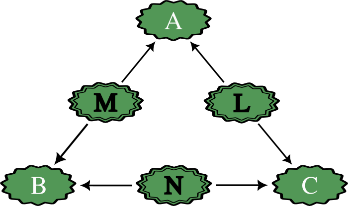
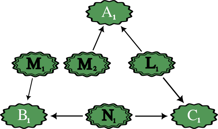
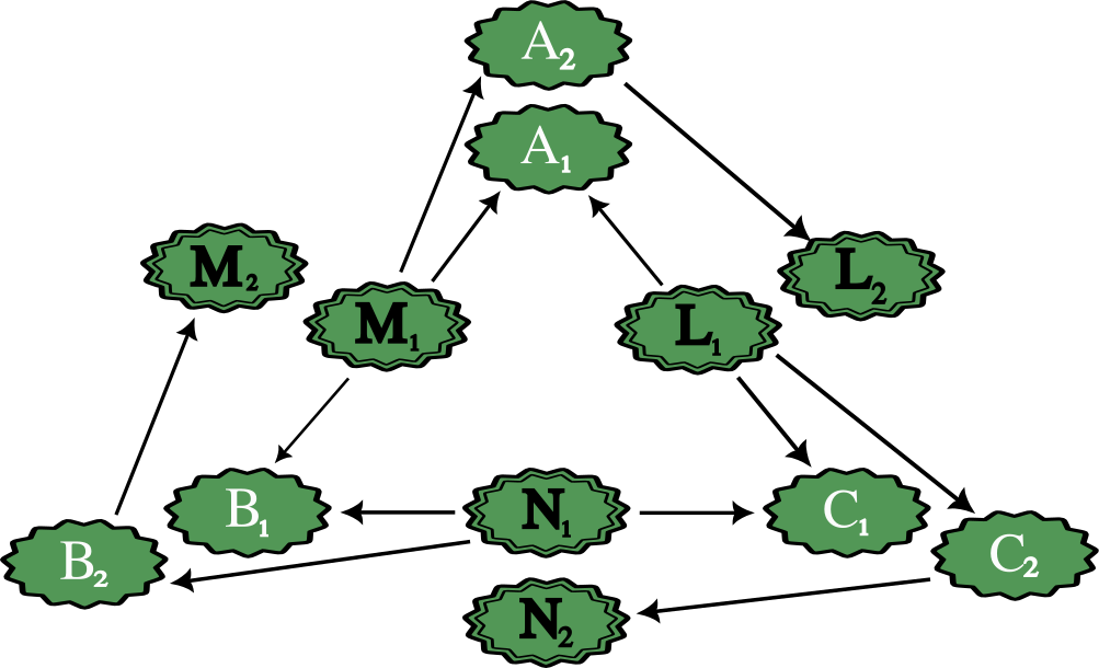
Figure 1: (a) The DAG describing the triangle scenario with quantum semantics for the visible and latent nodes. (b) The $AB$-Cut inflation of the triangle scenario. (c) The Spiral inflation of the triangle scenario. In all subfigures, visible nodes are indicated by a single-stroke border while latent nodes are indicated by a dual-stroke border. The textured edges and green colour of the nodes is to indicate that these are quantum systems rather than classical variables. The convention for the latter is seen in Fig. 2.

The main aim of this work is to showcase the utility of the inflation technique in conjunction with these operator inequalities for questions of compatibility of a joint quantum state with a given causal structure.

For illustrative purposes, we focus on the case of a tripartite system and the well-studied causal structure known as the triangle scenario, i.e., the structure that is depicted in Fig. 1(a). In particular, we use the Cut inflation of the triangle scenario, depicted in Fig. 1(b). Because the Cut inflation is a so-called nonfanout inflation (a notion that will be explained further on), it is applicable in the fully quantum case. Furthermore, for the Cut inflation, it is possible to leverage the marginal problem constraint derived by Hall [23] to obtain strong witnesses of incompatibility.

We will apply the technique for a few different choices of the dimensionalities of the visible quantum systems. We focus on the case of three qubits, but we consider also the case of three qutrits and the case of two qubits and a ququart. We also apply the technique not only to assessments of compatibility of pure states, but mixed states as well.

A number of benefits of this approach are worth elucidating here. Firstly, this technique is well-suited to numerically specified quantum states. For example, given a state $\rho$ that is specified by experimental state tomography or related methods, it is computationally simple to test compatibility for a specific choice of inflation and marginal inequality. A verdict of incompatibility could then witness the divergence of the actual causal structure of the experiment from the expected one, indicating a deficiency in the experimentalist’s understanding of the noise source of the set-up. This approach is also suitable for considering symbolically specified quantum states, as it utilizes analytic quantum marginal problem criteria, in contrast to the semidefinite programming approach of Ref. [26].

One motivation for studying compatibility of pure states with the triangle scenario (and $n$-node generalizations thereof where every subset of ${n{-}1}$ nodes have a latent common cause acting on them) is the definition of genuine $n$-partite entanglement proposed in Refs. [27, 26], based on entanglement under Local Operations and Shared Randomness (LOSR) rather than Local Operations and Classical Communication (LOCC). This definition is distinct from the conventional definition (the one based on biseparability), and overcomes various conceptual problems of the latter, as argued in Ref. [27]. Consider the case of $n=3$ for simplicity. The LOSR-based definition in this case is that a state is genuine tripartite entangled if it cannot be realized by resources of bipartite entanglement. More precisely, it is proposed that a genuine tripartite entangled state is one that cannot be realized by Local Operations and Shared Randomness with 2-way Shared Entanglement (LOSR2WSE). If the state to be prepared is pure, the shared randomness does not add any additional power, so we have that a pure state is genuinely tripartite entangled when it cannot be realized by Local Operations with 2-way Shared Entanglement (LO2WSE). But these operations are precisely what can be achieved in the triangle scenario, so a pure state is genuinely tripartite entangled when it is incompatible with the triangle scenario. Characterizing the boundary between pure states that are genuinely tripartite entangled and those that are not, therefore, provides a motivation for characterizing the boundary between pure states that are compatible with the triangle scenario and those that are not.

The notion of compatibility with the triangle scenario studied here is similar to but distinct from the notion of compatibility studied in Ref. [28] (where they refer to the triangle scenario as the independent triangle network). This is because the latter article considered only unitaries for the channels mapping the latent systems to the visible systems, rather than allowing arbitrary operations as we do here. In short, while we here consider state-preparability by Local Operations with 2-way Shared Entanglement, Ref. [28] considers state-preparability by Local Unitaries with 2-way Shared Entanglement (LU2WSE). Because LU2WSE $\subseteq$ LO2WSE, any state shown to be preparable by LU2WSE is also preparable by LO2WSE, but it is unclear whether or not the opposite implication holds. As such, it is possible that there is a strict inclusion relation between the set of LU2WSE-preparable states and the set of LO2WSE-preparable states. Consequently, any demonstration of incompatibility relative to LU2WSE does not necessarily imply incompatibility relative to LO2WSE. (See, however, the comments about the special case of pure states in Sec. IV.1.)

The remainder of this article is structured as follows.Section II provides a review of the necessary background on causal models, classical and quantum. Section III reviews the inflation technique for causal inference and shows how to leverage a particular family of operator inequalities related to the quantum marginal problem to derive constraints on compatibility of a quantum state with a causal structure. Application of these new constraints are presented in Section IV and Section V for qubit and higher-dimensional visible nodes respectively, with proofs presented in the appendices. Section VI discusses avenues for generalizing our results and conclusions.

II Preliminaries

II.1 Classical causal models

To begin with, consider what is arguably the simplest case: classical semantics for both the visible and the latent nodes. In the case of the triangle scenario, this is depicted inFig. 2(a). This means that both the visible and the latent nodes are associated to random variables. A joint state on the visible nodes is therefore a joint probability distribution over the associated random variables.

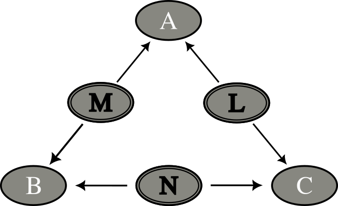
Figure 2: (a) The DAG describing the triangle scenario with classical semantics for the visible and latent nodes.

Let the DAG describing the causal structure be denoted $G$. Strictly speaking, we are considered a DAG with a classification of the nodes into visible and latent, a structure that was termed a partitioned DAG in Ref. [29]. Let the set of visible nodes of $G$ be denoted $\textsf{Vnodes}(G)$ and the set of latent nodes by $\textsf{Lnodes}(G)$. We also presume that the DAG is in a canonical form wherein latent nodes are necessarily exogenous.

For a classical causal model, the state on the visible nodes is a joint distribution $P_{\textsf{Vnodes}(G)}$. To specify a choice of parameter values in the causal model is to specify a distribution over each latent variable, i.e., a set $\{P_{L}:L\in\textsf{Lnodes}(G)\}$ (here, the cardinality of the set of values of each $L$ is assumed to be finite but allowed to be arbitrarily large, and a conditional probability for each visible variable given its causal parents $\{P_{A|\operatorname{Pa}(A)}:A\in\textsf{Vnodes}(G)\}$ (where the parental sets may include both visible and latent variables).

Definition 1 (Classical $G$-compatibility of a joint distribution.).

Consider a joint distribution $P_{\textsf{Vnodes}(G)}$ over the variables associated to the visible nodes of a causal structure $G$. We say that $P_{\textsf{Vnodes}(G)}$ is classically $G$-compatible if there exist a choice of the parameters in the classical causal model, that is, a choice of $\{P_{L}:L\in\textsf{Lnodes}(G)\}$ (distributions on the classical systems associated to the latent nodes) and of $\{P_{A|\operatorname{Pa}(A)}:A\in\textsf{Vnodes}(G)\}$ (conditional probability distributions defining a stochastic map whose inputs are the classical systems associated to the latent nodes and whose outputs are the classical systems associated to the visible nodes) such that these realize $P_{\textsf{Vnodes}(G)}$:

$$P_{\textsf{Vnodes}(G)}=\sum_{L\in\textsf{Lnodes}(G)}\prod_{A\in\textsf{Vnodes}(G)}P_{A|\operatorname{Pa}(A)}\prod_{L\in\textsf{Lnodes}(G)}P_{L}.$$ (1)

where $\sum_{L\in\textsf{Lnodes}(G)}$ indicates marginalisation over the variables assigned to latent nodes.

We now consider the concrete example of the triangle scenario. We use the notation for nodes presented in Fig. 2, that is, the visible nodes are denoted $A,B,C$ and the latent nodes are denoted $L,M,N$, and the variables associated to these nodes are denoted in the same manner as the nodes themselves. A joint distribution $P_{ABC}$ is compatible with the triangle scenario in a classical causal model if there exist choices of parameters $P_{A|LM},P_{B|MN},P_{C|LN},P_{L},P_{M}$, and $P_{N}$ such that

$$P_{ABC}=\sum_{LMN}P_{A|LM}P_{B|MN}P_{C|LN}P_{L}P_{M}P_{N}.$$ (2)

II.2 Quantum causal models

We now consider quantum causal models [9, 10, 11], where both the latent and visible nodes have quantum semantics.

In the case of the triangle scenario, this is depicted in Fig. 1(a).

For simplicity, we restrict our attention to causal structures wherein no two visible nodes appear in a cause-effect relationship (i.e., one visible node is never in the causal ancestry of another visible node) and wherein all latent nodes are exogenous (i.e., have no parents in the causal structure). This pair of restrictions together imply that the causal structure has just two layers: a layer of exogenous latent nodes and a layer of visible nodes. Such causal structures are sometimes termed networks [5, 18] and we shall adopt this terminology here.

In contrast with a classical causal model, which assigns a variable to each node (the important aspect of which is the cardinality of its set of values), a quantum causal model assigns a quantum system to each node (the important aspect of which is the dimension of Hilbert space associated to it). Consequently, to specify a choice of parameter values in a quantum causal model is to specify two types of parameters: (i) quantum states on the systems associated to the latent nodes (where the dimension of the Hilbert space associated to each latent node is assumed to be finite but allowed to be arbitrarily large), and (ii) quantum channels from these to the quantum systems associated to the visible nodes.

It follows that the entity whose compatibility with a causal structure is to be assessed is no longer a joint probability distribution, but a joint quantum state, specifically, $\rho_{\textsf{Vnodes}(G)}$, i.e., a positive trace-one operator on the Hilbert space $\bigotimes_{A\in\textsf{Vnodes}(G)}\mathcal{H}_{A}$.

Because of the no-broadcasting theorem in quantum theory [30], if a given latent node influences more than one visible node, one cannot imagine that the state of that node is broadcast to each of the children, as one could classically. The main differences between the definitions of the notion of a quantum causal model proposed in various works, such as Ref. [10] and Refs. [9, 11], relate to how to meet this challenge. However, because the compatibility problem allows the Hilbert spaces associated to the latent nodes to be of arbitrary dimensionality, and the differences between these approaches are inconsequential in this case; disagreements about the definition are not relevant to the compatibility problem. We here adopt the following approach: Suppose that the set of visible nodes that are children of a latent node $L$ are denoted $\textrm{Ch}(L)$. Then the Hilbert space associated to the latent node $L$, $\mathcal{H}_{L}$, is presumed to factorize into a set of Hilbert spaces indexed by its children. That is, $\mathcal{H}_{L}=\bigotimes_{A\in\textrm{Ch}(L)}\mathcal{H}_{L^{(A)}}$. The first type of parameter in the causal model is a quantum state $\rho_{L}$, i.e., a positive trace-one operator on the space of linear operators on the Hilbert space associated to $L$, $\rho_{L}\in\mathcal{L}(\mathcal{H}_{L})$. Given the factorization just described, the state $\rho_{L}$ can be conceptualized as $\rho_{L^{(1)},L^{(2)}\dots L^{(K)}}\in\mathcal{L}(\mathcal{H}_{L^{(1)}}\otimes\mathcal{H}_{L^{(2)}}\otimes\dots\otimes\mathcal{H}_{L^{(K)}})$, where $K$ is the cardinality of the set $\textrm{Ch}(L)$, and thus can describe correlations between the different subsystems of $L$.

The second type of parameter of the causal model specifies how each visible node depends on its causal parents. For each visible node $A\in\textsf{Vnodes}(G)$, one specifies a quantum channel whose output space is $\mathcal{L}(\mathcal{H}_{A})$, the operator space associated to $A$. Let $\widetilde{\textrm{Pa}}(A)$ be defined as $\{L^{(A)}:L\in\textrm{Pa}(A)\}$. That is, for each $L$ among the parents of $A$, include within $\widetilde{\textrm{Pa}}(A)$ only $L^{(A)}$, the subsystem of $L$ that influences $A$. Thus, whereas $\textrm{Pa}(A)$ describes the collection of latent nodes that are parents of $A$, $\widetilde{\textrm{Pa}}(A)$ describes the collection of subsystems of the latent nodes that have an influence on $A$. The input space of the quantum channel whose output space is $\mathcal{L}(\mathcal{H}_{A})$ is $\mathcal{L}(\mathcal{H}_{\widetilde{\textrm{Pa}}(A)})$. The channel can consequently be denoted $\mathcal{E}_{A|\widetilde{\textrm{Pa}}(A)}$. There is one such channel for each visible node.

We can now define what it means for a joint quantum state on the visible nodes of a network $G$ to be compatible with $G$ for quantum semantics of the latent nodes.

Definition 2 ($G$-compatibility in quantum causal models).

Let $G$ be a network and consider a joint quantum state $\rho_{\textsf{Vnodes}(G)}$ over the systems associated to the visible nodes of $G$. The state $\rho_{\textsf{Vnodes}(G)}$ is said to be $G$-compatible with the network $G$ within a quantum causal model if there exist a choice of the parameters of the model that realizes $\rho_{\textsf{Vnodes}(G)}$. More precisely, the joint state $\rho_{\textsf{Vnodes}(G)}$ is compatible with $G$ if, for each latent node $L\in\textsf{Lnodes}(G)$, there exists a choice of quantum state $\rho_{L}$, and for each visible node $A\in\textsf{Vnodes}(G)$, there exists a choice of quantum channel $\mathcal{E}_{A|\widetilde{\textrm{Pa}}(A)}$, such that

$$\rho_{\textsf{Vnodes}(G)}=\bigotimes_{A:A\in\textsf{Vnodes}(G)}\mathcal{E}_{A|\widetilde{\textrm{Pa}}(A)}\left(\bigotimes_{L:L\in\textsf{Lnodes}(G)}\rho_{L}\right).$$ (3)

Again, it is worthwhile to consider the concrete example of the triangle scenario, using the notational convention of Fig. 1(a). For these purposes, it is convenient to decompose the Hilbert spaces of each latent node into a pair of factors, labelled $l$ (left) and $r$ (right), i.e., $\mathcal{H}_{L}\cong\mathcal{H}_{L^{(l)}}\otimes\mathcal{H}_{L^{(r)}}$, $\mathcal{H}_{M}\cong\mathcal{H}_{M^{(l)}}\otimes\mathcal{H}_{M^{(r)}}$, $\mathcal{H}_{N}\cong\mathcal{H}_{N^{(l)}}\otimes\mathcal{H}_{N^{(r)}}$. A quantum state $\rho_{ABC}$ on $\mathcal{H}_{A}\otimes\mathcal{H}_{B}\otimes\mathcal{H}_{C}$ is triangle-compatible if there exist quantum states of the latent nodes $\varrho_{L}=\varrho_{L^{(l)}L^{(r)}}$, $\varrho_{M}=\varrho_{M^{(l)}M^{(r)}}$, $\varrho_{N}=\varrho_{N^{(l)}N^{(r)}}$ and quantum channels $\mathcal{E}_{A|L^{(r)}M^{(l)}}:\mathcal{H}_{L^{(r)}}\otimes\mathcal{H}_{M^{(l)}}\rightarrow\mathcal{H}_{A}$, $\mathcal{E}_{B|L^{(l)}N^{(r)}}:\mathcal{H}_{L^{(l)}}\otimes\mathcal{H}_{N^{(r)}}\rightarrow\mathcal{H}_{B}$, and $\mathcal{E}_{C|M^{(r)}N^{(l)}}:\mathcal{H}_{M^{(r)}}\otimes\mathcal{H}_{N^{(l)}}\rightarrow\mathcal{H}_{C}$ such that

$$\rho_{ABC}= \mathcal{E}_{A|L^{(r)}M^{(l)}}\otimes\mathcal{E}_{B|L^{(l)}N^{(r)}}$$ (4)

$$\otimes\mathcal{E}_{C|M^{(r)}N^{(l)}}(\varrho_{L^{(l)}L^{(r)}}\otimes\varrho_{M^{(l)}M^{(r)}}\otimes\varrho_{N^{(l)}N^{(r)}}).$$

As an aside, note that the partitioning of the latent systems into subsystems, each of which influences a different child node of the latent node, also provides an alternative way of defining a classical causal model. Take the triangle scenario as an example. The parametrization of the classical causal model that we provided earlier was $P_{A|LM},P_{B|MN},P_{C|LN},P_{L},P_{M}$, and $P_{N}$ such that

$$P_{ABC}=\sum_{LMN}P_{A|LM}P_{B|MN}P_{C|LN}P_{L}P_{M}P_{N}.$$ (5)

However, one can also partition each latent variable into a pair of latent variables and make each child depend on just one element of the pair. For instance, one defines $L=(L^{(l)},L^{(r)})$ and one makes $A$ depend only on $L^{(l)}$ and $C$ depend only on $L^{(r)}$. The parametrization of the classical causal model we obtain in this way is $P_{A|L^{(r)}M^{(l)}},P_{B|L^{(l)}N^{(r)}},P_{C|M^{(r)}N^{(l)}},P_{L^{(l)}L^{(r)}},P_{M^{(l)}M^{(r)}}$, and $P_{N^{(l)}N^{(r)}}$ such that

$$P_{ABC} =\sum_{LM,N}P_{A|L^{(r)}M^{(l)}}P_{B|L^{(l)}N^{(r)}}P_{C|M^{(r)}N^{(l)}}$$

$$\times P_{L^{(l)}L^{(r)}}P_{M^{(l)}M^{(r)}}P_{N^{(l)}N^{(r)}}$$ (6)

This second parametrization is clearly subsumed as a special case of the first. To see that the first is also subsumed as a special case of the second, it suffices to note that one can take $L^{(l)}$ and $L^{(r)}$ to be two copies of the $L$ of the first model and to take the distribution over $L^{(l)}L^{(r)}$ to be what one obtains from the distribution $P_{L}$ followed by applying a copy operation, so that $P_{L^{(l)}L^{(r)}}=P_{L}\delta_{L^{(r)},L}\delta_{L^{(l)},L}$. A similar observation holds for any causal model.

This demonstrates that one can recover a classical causal model from a quantum causal model by particularizing to density operators that are diagonal in some fixed product basis over the subsystems, since these are equivalent to probability distributions, and channels that act as stochastic maps relative to these bases, since these are equivalent to conditional probability distributions.

III Fully quantum inflation

III.1 A description of the technique

The inflation technique for causal inference [16] provides a method for resolving questions of causal compatibility. This method was inspired by ideas from the literature on Bell’s theorem, namely, derivations of Bell’s theorem that leverage results from the classical marginal problem.

At a high level, the inflation technique can be conceptualized as a means for converting facts about a marginal problem into facts about causal compatibility. We explore a particular version of this problem in the present paper, namely, how to make use of facts about the quantum marginal problem to obtain conclusions about causal compatibility between a causal structure and a joint quantum state.

In the following, we will generalize the inflation technique to the case of quantum causal models. Note that previous work allowed the latent nodes to be quantum, but a description of the inflation technique for the case where the visible nodes are quantum has not been provided previously. It is worth noting a subtlety regarding terminology at this point. Whether a causal model is termed ‘classical’ or ‘quantum’ refers to whether all the nodes are classical or all are quantum. The term ‘quantum inflation’, on the other hand, has been used [18] to describe the inflation technique wherein the latent nodes are quantum but the visible nodes are still classical (and in particular the case where one can treat fanout inflations). One consequently cannot refer to the inflation technique applied to quantum causal models as simply ‘quantum inflation’. Therefore, we introduce the term ‘fully quantum inflation’ to refer to the technique when both the latent and the visible nodes are quantum.

It is useful to contrast the classical and quantum cases. We will not, however, review the inflation technique for classical causal models. Rather, we will present the technique only for quantum causal models. The description of the technique for classical causal models can be recovered from the quantum one, as noted at the end of Sec. II.2, by simply restricting attention to density operators that are diagonal in some fixed product basis over the subsystems and channels that act as stochastic maps relative to these bases.

The first step in using the inflation technique consists of producing, from the original DAG $G$, a new DAG $G^{\prime}$, termed the inflation of $G$, in the following way (the reader is referred to [16] for a more complete treatment). The set of nodes of $G^{\prime}$, denoted $\mathsf{Nodes}(G^{\prime})$, are labelled in such a way that each can be associated to a node of $G$, with the possibility that more than one node of $G^{\prime}$ is associated to a single node in $G$. We refer to nodes of $G^{\prime}$ that are associated to a given node of $G$ as copies of the latter.

More precisely, we define a relation on sets of variables, denoted “$\sim$”, which we will term sameness up to copy-indices as follows: Supposing ${\bf X}\subseteq\mathsf{Nodes}(G)$ and ${\bf X}^{\prime}\subseteq\mathsf{Nodes}(G^{\prime})$, then ${\bf X}\sim{\bf X}^{\prime}$ if ${\bf X}^{\prime}$ contains exactly one copy of every node in ${\bf X}$.

Using this, we can define an equivalence relation among subgraphs. Namely, we write $\mathsf{SubDAG}_{G^{\prime}}({\bf X}^{\prime})\sim\mathsf{SubDAG}_{G}({\bf X})$ if ${\bf X}\sim{\bf X}^{\prime}$ and an edge is present between two nodes in ${\bf X}^{\prime}$ within $\mathsf{SubDAG}_{G^{\prime}}({\bf X}^{\prime})$ whenever it is present between the two associated nodes in ${\bf X}$ within $\mathsf{SubDAG}_{G}({\bf X})$.

The set of DAGs that we refer to as the inflations of $G$, denoted $\mathsf{Inflations}(G)$, is defined as follows: $G^{\prime}\in\mathsf{Inflations}(G)$ if and only if, for all $A\in\mathsf{Nodes}(G)$, and all $A_{i}\in\mathsf{Nodes}(G^{\prime})$ the ancestral subgraph of $A_{i}$ in $G^{\prime}$ is equivalent up to copy indices to the ancestral subgraph of $A$ in $G$,

$$\mathsf{ansubgraph}_{G^{\prime}}(A_{i})\sim\mathsf{ansubgraph}_{G}(A).$$ (7)

To explain this further, let us consider the inflation used in the remainder of this work, namely the $AB$-Cut inflation of the triangle scenario, depicted in Fig. 1(b). In this case, the inflated DAG contains just a single copy of each of the visible nodes, $A,B,C$, and a single copy of two of the latent nodes, namely, $L$ and $N$ but two copies of the latent node $M$. The latter are denoted by $M_{1}$ and $M_{2}$, while the former are denoted by $A_{1},B_{1},C_{1},L_{1},N_{1}$. Consider next the requirement of matching the ancestral subgraphs of visible nodes. The ancestry of each of the visible nodes in the original triangle consists only of the node’s parents, so that the ancestral sub-DAG of node $A$ is the $v$-shaped “collider” DAG with arrows pointing from latent nodes $L$ and $M$ to $A$ (and similarly for $B$ with parents $L,N$ and for $C$ with parents $M,N$). In the Cut inflation, the situation is the same: the visible node $A_{1}$ has ancestry given by the $v$-shaped DAG with parents $L_{1}$ and $M_{2}$, $B_{1}$ has parents $M_{1}$ and $N_{1}$, and $C_{1}$ has parents $L_{1}$ and $N_{1}$. By removing the copy-indices (the subscripts) these ancestral sub-DAGs exactly match those of $A$, $B$ and $C$.

Up until this point, we have not stipulated whether we are considering a classical or quantum causal model (or indeed a causal model for some other generalized probabilistic theory), a distinction that we refer to as the semantics of the causal model. The semantics specifies the nature of the parameters of the causal model. From this point on, however, what we say is specific to quantum causal models. As noted above, the case of classical causal models can be recovered by restricting attention to density operators that are diagonal relative to some fixed product basis over the subsystems and channels that act as stochastic maps relative to this basis.

We now introduce a map from the parameters of a causal model on $G$, denoted par, to the parameters of a causal model on $G^{\prime}$ (an inflation of $G$), denoted par^′. In other words, we describe how inflation acts on the parameters of a model. We denote this map from par to par^′ by $\mathsf{Inflation}_{G\to G^{\prime}}$.

The map $\mathsf{Inflation}_{G\to G^{\prime}}$ taking a choice of parameters on $G$ to a choice of parameters on the $G^{\prime}\in\textsf{Inflations}(G)$ is defined by the following conditions: (i) For every visible node $A_{i}$ in $G^{\prime}$, the quantum channel relating $A_{i}$ to its parents within $G^{\prime}$ is the same as the quantum channel relating $A$ to its parents within $G$,

$$\forall A_{i}\in\textsf{Vnodes}(G^{\prime}):\;\mathcal{E}_{A_{i}|\widetilde{\textrm{Pa}}_{G^{\prime}}(A_{i})}=\mathcal{E}_{A|\widetilde{\textrm{Pa}}_{G}(A)}.$$ (8)

(ii) For every latent node $L_{j}$ in $G^{\prime}$, the state on $L_{j}$ is the same as the state on $L$ in $G$,

$$\forall L_{j}\in\textsf{Lnodes}(G^{\prime}):\;\rho_{L_{j}}=\rho_{L}.$$ (9)

One of the key concepts in the inflation technique is that of a set of visible nodes in $G^{\prime}$ for which one can find a copy-index-equivalent set in the original DAG $G$ with a copy-index-equivalent ancestral subgraph. Such subsets of the visible nodes of $G^{\prime}$ are referred to as injectable sets. More precisely, a set of visible nodes of $G^{\prime}$, $\bm{U}^{\prime}\subset\textsf{Vnodes}(G^{\prime})$, is an injectable set, i.e., $\bm{U}^{\prime}\in\textsf{InjectableSets}(G^{\prime})$, if and only if there exists a set of visible nodes of $G$, $\bm{U}\subset\textsf{Vnodes}(G)$ that is copy-index equivalent to ${\bf U}^{\prime}$, $\bm{U}^{\prime}\sim\bm{U}$, such that the ancestral subgraph of $\bm{U}^{\prime}$ in $G^{\prime}$ is equivalent up to copy indices to the ancestral subgraph of $\bm{U}$ in $G$,

$$\textsf{ansubgraph}_{G^{\prime}}(\bm{U}^{\prime})\sim\textsf{ansubgraph}_{G}(\bm{U}).$$ (10)

Note that by the definition of an inflation DAG, every singleton set of visible nodes is an injectable set.

It is constructive to see an explicit example. We will consider the case of the $AB$-Cut inflation of the triangle DAG, since this will be relevant further on. In this case, one can easily see that the set $\{A_{1},C_{1}\}$ is injectable. This follows from the fact that the ancestral subgraph of $\{A_{1},C_{1}\}$ in the $AB$-Cut inflation DAG consists of the sub-DAG formed by the nodes $\{A_{1},C_{1},L_{1},M_{1},N_{1}\}$ and the edges between these, and this is equivalent, up to dropping of copy-indices, to the ancestral subgraph of $\{A,C\}$ in the triangle scenario DAG triangle scenario, namely, the sub-DAG formed by the nodes $\{A,C,L,M,N\}$ and the edges between these. The set $\{B_{1},C_{1}\}$ is also injectable by a parallel argument. The set $\{A_{1},B_{1}\}$, on the other hand, is not injectable. This is because $A_{1}$ and $B_{1}$ have no common ancestor in the $AB$-Cut inflation DAG, where $M_{1}$ influences only $A_{1}$ and $M_{2}$ influences only $B_{1}$, whereas $M$ is part of both of their ancestral subgraphs in the triangle scenario.

Those sets of visible nodes in the original DAG $G$ that are copy-index-equivalent to an injectable set in $G^{\prime}$ we refer to as images of the injectable sets under the dropping of copy-indices, and denote as $\textsf{ImagesInjectableSets}(G)$. Clearly, $\bm{U}\in\textsf{ImagesInjectableSets}(G)$ if and only if there exists $\bm{U}^{\prime}\subseteq\textsf{InjectableSets}(G^{\prime})$ such that $\bm{U}\sim\bm{U}^{\prime}$.

We finally come to the result that captures why the inflation map is relevant for the compatibility problem.

Proposition 1.

Let the DAG $G^{\prime}$ be an inflation of the DAG $G$. Let $S^{\prime}\subseteq\mathsf{InjectableSets}(G^{\prime})$ be a collection of injectable sets, and let $S\subseteq\mathsf{ImagesInjectableSets}(G)$ be the images of this collection under the dropping of copy-indices. If the family of states $\{\rho_{\bm{U}}:\bm{U}\in S\}$ is compatible with $G$, then the corresponding family of states $\{\rho_{\bm{U}^{\prime}}:\bm{U}^{\prime}\in S^{\prime}\}$, defined via $\rho_{\bm{U}^{\prime}}=\rho_{\bm{U}}$ for $\bm{U}^{\prime}\sim\bm{U}$, is compatible with $G^{\prime}$.

Proof.

From the assumption that the family of states $\{\rho_{\bm{U}}:\bm{U}\in S\}$ is compatible with $G$, one infers that there exists a choice of parameters on $G$, par, that realizes $\rho_{\bm{U}}$ on each $\bm{U}\in S$. But then the parameters on $G^{\prime}$ given by $\texttt{par}^{\prime}=\textsf{Inflation}_{G\rightarrow G^{\prime}}(\texttt{par})$, realize $\rho_{\bm{U}^{\prime}}=\rho_{\bm{U}}$ on each $\bm{U}^{\prime}\in S^{\prime}$. Consequently, the family of states $\{\rho_{\bm{U}^{\prime}}:\bm{U}^{\prime}\in S^{\prime}\}$ that is defined via $\rho_{\bm{U}^{\prime}}=\rho_{\bm{U}}$ for $\bm{U}^{\prime}\sim\bm{U}$, is compatible with $G^{\prime}$. ∎

Next, it is useful to define the notion of a causal compatibility inequality.

Let $G$ be a causal structure and let $S$ be a family of subsets of the visible nodes of $G$. Let $I_{S}$ denote an inequality that operates on the corresponding family of states, $\{\rho_{\bm{U}}:\bm{U}\in S\}$. Then $I_{S}$ is a causal compatibility inequality for the causal structure $G$ (or a $G$-compatibility inequality for short) whenever it is satisfied by every family of states $\{\rho_{\bm{U}}:\bm{U}\in S\}$ that is compatible with $G$.

Note that while violation of a causal compatibility inequality for $G$ witnesses the incompatibility of a state with the causal structure $G$, satisfaction of the inequality does not guarantee compatibility: satisfaction of the inequality merely provides a necessary condition for compatibility.

Inflation provides a means of “pulling back” causal compatibility inequalities from the inflation DAG $G^{\prime}$ to the original DAG $G$. This is formalized in the following corollary of Proposition 1.

Corollary 1.

Suppose that $G^{\prime}$ is an inflation of $G$. Let $S^{\prime}\subseteq\mathsf{InjectableSets}(G^{\prime})$ be a family of injectable sets and $S\subseteq\mathsf{ImagesInjectableSets}(G)$ the family consisting of the images of members of $S^{\prime}$ under the dropping of copy-indices. Let $I_{S^{\prime}}$ be a causal compatibility inequality for $G^{\prime}$ operating on families of states $\{\rho_{\bm{U}^{\prime}}:\bm{U}^{\prime}\in S^{\prime}\}$. Define an inequality $I_{S}$ as follows: in the functional form of $I_{S^{\prime}}$, replace every occurrence of a term $\rho_{\bm{U}^{\prime}}$ by $\rho_{\bm{U}}$ for the unique $\bm{U}\in S$ such that $\bm{U}\sim\bm{U}^{\prime}$. Then $I_{S}$ is a causal compatibility inequality for $G$ operating on families of states $\{\rho_{\bm{U}}:\bm{U}\in S\}$.

Proof.

The assumption that $I_{S^{\prime}}$ is a causal compatibility inequality for $G^{\prime}$ implies that if a family of states $\{\rho_{\bm{U}^{\prime}}:\bm{U}^{\prime}\in S^{\prime}\}$ is compatible with $G^{\prime}$, then it satisfies the inequality $I_{S^{\prime}}$. By Proposition 1, if the family of states $\{\rho_{\bm{U}}:\bm{U}\in S\}$ is compatible with $G$, then the corresponding family of states $\{\rho_{\bm{U}^{\prime}}:\bm{U}^{\prime}\in S^{\prime}\}$, defined via $\rho_{\bm{U}^{\prime}}=\rho_{\bm{U}}$ for $\bm{U}^{\prime}\sim\bm{U}$, is compatible with $G^{\prime}$. Together, these two facts imply that if the family of states $\{\rho_{\bm{U}}:\bm{U}\in S\}$ is compatible with $G$, then the family of states $\{\rho_{\bm{U}^{\prime}}:\bm{U}^{\prime}\in S^{\prime}\}$, defined via $\rho_{\bm{U}^{\prime}}=\rho_{\bm{U}}$ for $\bm{U}^{\prime}\sim\bm{U}$ satisfies the inequality $I_{S^{\prime}}$. Since $I_{S}$ is defined as having the functional form of $I_{S^{\prime}}$, where every occurrence of a term $\rho_{\bm{U}^{\prime}}$ is replaced by $\rho_{\bm{U}}$ for the unique $\bm{U}\in S$ such that $\bm{U}\sim\bm{U}^{\prime}$, we infer that the family of states $\{\rho_{\bm{U}}:\bm{U}\in S\}$ satisfies $I_{S}$. ∎

Note that all of these results are simply straightforward quantum generalizations of the ones presented in Ref. [16] for the case of classical causal models.

III.1.1 The distinction between fanout and nonfanout inflations

An inflation is called fanout if it contains a latent node that influences visible nodes that are copy-index equivalent, that is, if it contains a latent node that influences more than one copy of a visible node from the original DAG. Otherwise, the inflation is termed nonfanout. For the triangle scenario, an example of a fanout inflation is the spiral inflation, depicted in Fig. 1(c), while an example of a nonfanout inflation is the Cut inflation, depicted in Fig. 1(b).

If one is considering the causal compatibility problem in quantum causal models, then it is not clear how to make use of a fanout inflation. In particular, the interpretation of a fanned-out latent node cannot be that it is copied and made to influence each of several copy-index-equivalent children, because the quantum no-broadcasting theorem prohibits such copying [30]. As such, we here restrict attention to nonfanout inflations when deriving causal compatibility constraints in the case of quantum causal models.

In the case where the visible nodes are classical, so that the compatibility problem concerns a joint probability distribution over the visible nodes, then it is an interesting problem to determine, for a given causal structure, whether there is a difference between what can be realized with classical versus quantum latent nodes. Nonfanout inflations derive constraints on compatible distributions that hold for both types of latent nodes. It is only with fanout inflations that one can derive constraints that can separate the cases of classical and quantum latents. For the Bell scenario, for instance, it is a fanout inflation that allows one to derive Bell inequalities, which are the constraints that establish the existence of a quantum-classical gap in this case.

It is worth noting that some causal structures do not admit of any nontrivial nonfanout inflations. For example, the causal structure known as the bilocal scenario (see e.g., [20]) is such an example that is moreover a member of the class of causal structures considered here (i.e., it is a network).

III.2 Example of Cut inflation of triangle scenario: classical case

As noted above, one obtains a description of how inflation can be used to derive causal compatibility inequalities for classical causal models by simply restricting to density operators that are diagonal relative to some fixed product basis over the subsystems and channels that act as stochastic maps relative to this basis.

In this article, we will focus on using the inflation technique to derive causal compatibility constraints for the triangle scenario using the cut inflation. We do so first for classical causal models, i.e., using the classical version of the inflation technique, in order to facilitate a comparison with the case of quantum causal models which is our main focus.

III.2.1 Leveraging classical marginal inequalities

We consider the $AB$-Cut inflation of the triangle scenario, depicted in Fig. 1(b). As noted earlier, the injectable sets of visible nodes in this case are, in addition to all the singleton sets, the two-node sets $\{A_{1},C_{1}\}$ and $\{B_{1},C_{1}\}$. By the classical version of 1, which follows from taking all density operators to be diagonal in some product basis (see corollary 6 of Ref. [16]), any causal compatibility inequality for the inflation DAG that involves only the marginal contexts $\{A_{1}\},\{B_{1}\},\{C_{1}\},\{A_{1},C_{1}\}$ and $\{B_{1},C_{1}\}$ defines (by dropping of copy-indices) a causal compatibility inequality for the original DAG. We turn, therefore, to the question of how to leverage results from the classical marginal problem to derive causal compatibility inequalities on the inflation DAG that are of this type.

We begin by recalling the classical marginal problem on a set of variables ${\bf V}$. Any strict subset of variables is termed a marginal context. The set of all marginal contexts, which is simply the power set of the set ${\bf V}$, which we denote by $2^{\bf V}$. An instance of the classical marginal problem is to determine, for a given set of marginal contexts $S\subseteq 2^{\bf V}$, and a given set of distributions on each of these contexts, $\{Q_{\bf X}:{\bf X}\in S\}$, whether there is a joint distribution $Q_{\bf V}$ such that each of the $Q_{\bf X}$ is recovered as the marginal of $Q_{\bf V}$ on ${\bf X}$, i.e., such that $Q_{\bf X}=\sum_{{\bf V}/{\bf X}}Q_{\bf V}$. In this case, we say that the set of distributions $\{Q_{\bf X}:{\bf X}\in S\}$ satisfy marginal compatibility.

The most obvious constraint that a set $\{Q_{\bf X}:{\bf X}\in S\}$ must satisfy in order to be marginally compatible is termed the equimarginal property and asserts that for any inclusion relation holding among the marginal contexts, i.e., ${\bf X}^{\prime},{\bf X}\in S$ such that ${\bf X}^{\prime}\subset{\bf X}$, we require $Q_{\bf X^{\prime}}:=\sum_{{\bf X}/{\bf X^{\prime}}}Q_{\bf X}$. This constraint is straightforward to check, so we will restrict our attention to nontrivial constraints. That is, we will only ask about the marginal compatibility of sets $\{Q_{\bf X}:{\bf X}\in S\}$ that satisfy the equimarginal property.

For our example, the set of variables is ${\bf V}=\{A,B,C\}$, and the set of marginal contexts of interest is the powerset of ${\bf V}$ excluding ${\bf V}$ itself, so that $S=2^{\bf V}\!\setminus\!{\bf V}:=\{\{A\},\{B\},\{C\},\{AB\},\{AC\},\{BC\}\}$. The input to our classical marginal problem in this case is an equimarginal set of distributions $\{Q_{\bf X}:{\bf X}\in 2^{\bf V}\!\setminus\!{\bf V}\}=\{Q_{A},Q_{B},Q_{C},Q_{AB},Q_{AC},Q_{BC}\}$.

A necessary condition for such an equimarginal family of distributions to be marginally compatible is that the following inequality be satisfied [25]:

$$\textbf{1}-Q_{A}-Q_{B}-Q_{C}+Q_{AB}+Q_{AC}+Q_{BC}\geq\textbf{0},$$ (11)

where the distributions appearing here are conceptualized as functions over the full sample space, $\bf{1}$ denotes the function that takes the value 1 everywhere, and $\bf{0}$ denotes the function that takes the value 0 everywhere. We refer to this as a marginal compatibility inequality.

To emphasize that this is to be conceptualized as an inequality on a family of distributions $\{Q_{\bf X}:{\bf X}\in 2^{\bf V}\!\setminus\!{\bf V}\}$, It is useful to write it as:

$$\Delta(\{Q_{\bf X}:{\bf X}\in 2^{\bf V}\!\setminus\!{\bf V}\})\geq\textbf{0}.$$ (12)

where $\Delta(\{Q_{\bf X}:{\bf X}\in 2^{\bf V}\!\setminus\!{\bf V}\}):=\textbf{1}-Q_{A}-Q_{B}-Q_{C}+Q_{AB}+Q_{AC}+Q_{BC}$.

Also, if one evaluates this functional inequality at $A=a,B=b,C=c$ for each set of values $a,b,c$, one obtains a set of inequalities on the real parameters appearing in these distributions, specifically,

$$\forall a,b,c: 1-Q_{A}(a)-Q_{B}(b)-Q_{C}(c)$$

$$+Q_{AB}(ab)+Q_{AC}(ac)+Q_{BC}(bc)\geq 0.$$ (13)

If the constraint is presented in this form, then we have a set of inequalities, rather than a single inequality. In this case, we term them marginal compatibility inequalities (plural).

Now consider a distribution $P_{A_{1}B_{1}C_{1}}$ on the variables appearing in the $AB$-Cut inflation DAG, namely, $A_{1}$, $B_{1}$ and $C_{1}$. The marginal compatibility inequality above implies that

$$\textbf{1}-P_{A_{1}}-P_{B_{1}}-P_{C_{1}}+P_{A_{1}B_{1}}+P_{A_{1}C_{1}}+P_{B_{1}C_{1}}\geq 0.$$ (14)

Note that this constraint follows simply from classical probability theory and has nothing to do with the causal structure of the $AB$-Cut inflation DAG. However, we will now combine it with a constraint that does follow from this causal structure.

Specifically, we consider the $d$-separation relations among the visible nodes. In the case of the $AB$-Cut inflation, there is one such relation, namely, that $A_{1}$ and $B_{1}$ are $d$-separated given the empty set. It follows that for any distribution $P_{A_{1}B_{1}C_{1}}$ that is compatible with the $AB$-Cut inflation DAG, we require

$$P_{A_{1}B_{1}}=P_{A_{1}}P_{B_{1}}.$$ (15)

To get a nontrivial causal compatibility inequality on the marginals of $P_{A_{1}B_{1}C_{1}}$, it suffices to combine the equality constraint of Eq. (15) with the marginal compatibility inequality of Eq. (11) to obtain:

$$\textbf{1}-P_{A_{1}}-P_{B_{1}}-P_{C_{1}}+P_{A_{1}}P_{B_{1}}+P_{A_{1}C_{1}}+P_{B_{1}C_{1}}\geq\textbf{0}.$$ (16)

(Note the difference to Eq. (14), namely, that $P_{A_{1}}P_{B_{1}}$ appears in place of $P_{A_{1}B_{1}}$.)

From this, we can infer a causal compatibility inequality for the triangle scenario DAG. It suffices to note that the inequality of Eq. (16) is a polynomial function of $P_{A_{1}},P_{B_{1}},P_{C_{1}},P_{A_{1}C_{1}}$ and $P_{B_{1}C_{1}}$ and that these are all marginals on injectable sets of visible nodes in the inflation DAG. By 1, we infer that the inequality having the same functional form as Eq. (16) but where $A_{1}$, $B_{1}$ and $C_{1}$ are replaced by $A$, $B$ and $C$ respectively, namely,

$$\textbf{1}-P_{A}-P_{B}-P_{C}+P_{A}P_{B}+P_{AC}+P_{BC}\geq\textbf{0}.$$ (17)

is a causal compatibility inequality for the triangle scenario in terms of the marginals $P_{A},P_{B},P_{C},P_{AC},$ and $P_{BC}$ of $P_{ABC}$. If a given joint distribution $P_{ABC}$ violates the inequality of Eq. (17), then it is incompatible with the triangle scenario. Following the terminology of a “$G$-compatibility inequality” introduced above, it is appropriate to refer to such an inequality on $P_{ABC}$ as a triangle-compatibility inequality.

One can of course consider Cut Inflations where the Cut is between $B$ and $C$ or between $A$ and $C$, rather than being between $A$ and $B$. We get analogous inequalities for each case, namely, for each $x,y,z\in\{A,B,C\}$ such that $x\neq y\neq z$,

$$\textbf{1}-P_{x}-P_{y}-P_{z}+P_{x}P_{y}+P_{xz}+P_{yz}\geq\textbf{0}.$$ (18)

A violation of any of these inequalities suffices to demonstrate triangle-incompatibility. In general, it will be clear from the context and the notation which inequality is being used (such as via the use of subscripts as in, e.g., (19) below).

Because the inequality of Eq. (18) expresses a necessary condition on the joint distribution $P_{ABC}$ for triangle-compatibility using the $xy$-Cut inflation, it is useful to write it as

$$I_{xy}(P_{ABC})\geq\bf{0},$$ (19)

where

$$I_{xy}(P_{ABC}):=\textbf{1}-P_{x}-P_{y}-P_{z}+P_{x}P_{y}+P_{xz}+P_{yz}$$

where $P_{x}$ is the marginal on the singleton set $x$, $P_{xz}$ is the marginal on the two-variable set $xz$, etcetera.

III.2.2 Some distributions whose triangle-incompatibility is witnessed

We now explore some of the conclusions that can be inferred from this triangle-compatibility inequality.

As a simple example, consider the following tripartite distribution, which we will refer to as the GHZ distribution (because of its similarity with the GHZ state in quantum theory):

$$P^{(\rm GHZ)}=\frac{1}{2}\left([000]_{ABC}+[111]_{ABC}\right),$$ (20)

where $[abc]_{ABC}$ denotes the point distribution wherein all the probabilistic weight is on $A=a$, $B=b$, and $C=c$. It is straightforward to see that $P^{\rm GHZ}_{ABC}$ violates a triangle-compatibility inequality. For example, using Eq. 17 and taking $A=0,B=0,C=1$, we find that the left-hand-side evaluates to $1-\tfrac{1}{2}-\tfrac{1}{2}-\tfrac{1}{2}+\tfrac{1}{4}+0+0=-\tfrac{1}{4}$. Since this is negative, the inequality is violated. It follows that the GHZ distribution is incompatible with the triangle scenario.

It is worth recalling that violations of a $G$-compatibility inequality by a distribution witnesses the incompatibility of that distribution with the causal structure $G$, but satisfaction of such inequalities by a distribution does not guarantee that it is compatible. A good example of this is the following distribution,

$$P^{({\rm W})}=\frac{1}{3}\left([100]_{ABC}+[010]_{ABC}+[001]_{ABC}\right).$$ (21)

which is termed the “W distribution”. $P^{\rm W}_{ABC}$ can easily be verified to satisfy the triangle-compatibility inequalities (satisfaction of the inequality for any of the Cuts implies satisfaction of the inequalities for the other Cuts due to the symmetries in the distribution), but it is nonetheless incompatible with the triangle scenario

Triangle-incompatibility of the W distribution is established in Ref. [16] using the Spiral inflation of the triangle scenario, which is depicted in Fig. 1(c).

III.3 Example of Cut inflation of triangle scenario: quantum case

Again, we consider the $AB$-Cut inflation of the triangle scenario, depicted in Fig. 1(b). Analogously to the classical case, 1 guarantees that if we can identify a causal compatibility inequality on the inflation DAG that involves only the marginal contexts $\{A_{1}\},\{B_{1}\},\{C_{1}\},\{A_{1},C_{1}\}$ and $\{B_{1},C_{1}\}$, then dropping the copy-indices yields a causal compatibility inequality for the triangle scenario. We find such a causal compatibility inequality on the inflation DAG by leveraging the results from the quantum marginal problem. This is the sense in which the fully quantum inflation technique allows questions of causal compatibility to be related to quantum marginal problems, allowing progress on the latter to be brought to bear on the former.

III.3.1 Leveraging quantum marginal inequalities

This subsection presents a family of operator inequalities describing solutions to a particular instance of the quantum marginal problem and demonstrates how these can be leveraged in fully quantum inflation. Specifically, the extra constraints enforced by the causal structure of the inflation DAG (such as factorization constraints) can be substituted into these operator inequalities to yield modified operator inequalities that constitute causal compatibility inequalities for the inflation DAG.

The quantum version of the marginal problem is defined precisely as the classical version, but where we consider joint quantum states rather than joint probability distributions, and marginalization corresponds to the partial trace operation. Consequently, if ${\bf V}$ denotes the full set of quantum systems under consideration, an instance of the quantum marginal problem is to determine, for a given set of marginal contexts $S\subseteq 2^{\bf V}$, and a given set of quantum states on each of these contexts, $\{\sigma_{\bf X}:{\bf X}\in S\}$, whether there is a joint quantum state $\sigma_{\bf V}$ such that each of the $\sigma_{\bf X}$ is recovered as the marginal of $\sigma_{\bf V}$ on ${\bf X}$, i.e., such that $\sigma_{\bf X}={\rm Tr}_{{\bf V}/{\bf X}}\sigma_{\bf V}$. In this case, we say that the set of states $\{\sigma_{\bf X}:{\bf X}\in S\}$ satisfy marginal compatibility.

In Ref. [23], Hall introduced a necessary condition that the marginals of any quantum state on a (finite-dimensional) composite Hilbert space consisting of an odd number of subsystems must satisfy (c.f. [23, Thm 1] and the discussion thereafter). Suppose ${\bf V}$ denotes a set of quantum systems and let $\sigma_{\bf X}\in\mathcal{L}(\bigotimes_{X\in{\bf X}}\mathcal{H}_{X})$ denote a joint quantum state on ${\bf X}\subseteq{\bf V}$ (i.e., a positive semidefinite operator with unit trace). The necessary condition on a set $\{\sigma_{\bf X}:{\bf X}\in 2^{\bf V}\!\setminus\!{\bf V}\}$ of states to be the marginals of a single state $\sigma_{\bf V}$ when the set ${\bf V}$ is of odd cardinality is the following operator inequality:

$$\Delta(\{\sigma_{\bf X}:{\bf X}\in 2^{\bf V}\!\setminus\!{\bf V}\})\geq 0$$ (22)

where

$$\Delta(\{\sigma_{\bf X}:{\bf X}\in 2^{\bf V}\!\setminus\!{\bf V}\}):=\sum_{{\bf X}\in 2^{\bf V}\!\setminus\!{\bf V}}(-1)^{|{\bf X}|}\sigma_{\bf X}\otimes\mathbb{1}_{{\bf V}\!\setminus\!{\bf X}},$$ (23)

with $|{\bf X}|$ denoting the cardinality of the set ${\bf X}$ and with $\geq$ denoting the standard partial order relation over Hermitian operators (i.e., $M\geq N$ if and only if $M-N$ is a positive semi-definite operator), so that an operator inequality of the form $O\geq 0$ signifies that $O$ is positive semidefinite.

In this work, we focus on the case of ${\bf V}=\{A,B,C\}$, and thus on the operator

$$\Delta (\{\sigma_{\bf X}:{\bf X}\in 2^{\bf V}\!\setminus\!{\bf V}\})$$

$$=\mathbb{1}-\sigma_{A}\otimes\mathbb{1}_{BC}-\sigma_{B}\otimes\mathbb{1}_{AC}-\sigma_{C}\otimes\mathbb{1}_{AB}$$

$$\quad+\sigma_{AB}\otimes\mathbb{1}_{C}+\sigma_{AC}\otimes\mathbb{1}_{B}+\sigma_{BC}\otimes\mathbb{1}_{A}.$$ (27)

It is convenient to suppress tensor products with identity operators and write simply

$$\Delta (\{\sigma_{\bf X}:{\bf X}\in 2^{\bf V}\!\setminus\!{\bf V}\})$$

$$=\mathbb{1}-\sigma_{A}-\sigma_{B}-\sigma_{C}+\sigma_{AB}+\sigma_{AC}+\sigma_{BC}.$$ (28)

Because ${\bf V}$ is of odd cardinality, we infer from Hall’s result that $\Delta(\{\sigma_{\bf X}:{\bf X}\in 2^{\bf V}\!\setminus\!{\bf V}\})$ must be positive semidefinite, so that

$$\mathbb{1}-\sigma_{A}-\sigma_{B}-\sigma_{C}+\sigma_{AB}+\sigma_{AC}+\sigma_{BC}\geq 0.$$ (29)

In this form, the operator inequality is clearly the quantum counterpart of Eq. (11). We refer to it as a quantum marginal compatibility inequality.

Now consider a state $\rho_{A_{1}B_{1}C_{1}}$ on the systems that appear in the $AB$-Cut inflation DAG, namely, $A_{1}$, $B_{1}$ and $C_{1}$. The quantum marginal compatibility inequality above implies that

$$\mathbb{1}-\rho_{A_{1}}-\rho_{B_{1}}-\rho_{C_{1}}+\rho_{A_{1}B_{1}}+\rho_{A_{1}C_{1}}+\rho_{B_{1}C_{1}}\geq 0.$$ (30)

As with the constraint of Eq. (14) in the classical case, this constraint has nothing to do with the causal structure of the $AB$-Cut inflation DAG, but we can combine it with such a constraint to obtain a causal compatibility inequality.

Again, we leverage the fact that in the $AB$-Cut inflation DAG, $A_{1}$ and $B_{1}$ are d-separated given the empty set, which is to say that there is no common cause acting on $A_{1}$ and $B_{1}$. It follows that any state $\rho_{A_{1}B_{1}C_{1}}$ that is compatible with this DAG must satisfy

$$\rho_{A_{1}B_{1}}=\rho_{A_{1}}\otimes\rho_{B_{1}}.$$ (31)

To get a nontrivial causal compatibility inequality for the $AB$-Cut inflation DAG, we combine the equality constraint of Eq. (31) with the quantum marginal compatibility inequality of Eq. (30) to obtain:

$$\mathbb{1}-\rho_{A_{1}}-\rho_{B_{1}}-\rho_{C_{1}}+\rho_{A_{1}}\otimes\rho_{B_{1}}+\rho_{A_{1}C_{1}}+\rho_{B_{1}C_{1}}\geq\textbf{0}.$$ (32)

Finally, we can use this together with 1 to obtain a causal compatibility inequality for the original triangle scenario DAG. Because the inequality is a polynomial function of $\rho_{A_{1}},\rho_{B_{1}},\rho_{C_{1}},\rho_{A_{1}C_{1}}$ and $\rho_{B_{1}C_{1}}$ and because these are all marginals on injectable sets of visible nodes in the inflation DAG, the inequality having the same functional form as Eq. (16) but where $A_{1}$, $B_{1}$ and $C_{1}$ are replaced by $A$, $B$ and $C$ respectively,

$$\mathbb{1}-\rho_{A}-\rho_{B}-\rho_{C}+\rho_{A}\otimes\rho_{B}+\rho_{AC}+\rho_{BC}\geq\textbf{0}.$$ (33)

is a causal compatibility inequality for the triangle scenario.

We refer to this operator inequality as a triangle-compatibility inequality for the quantum state $\rho_{ABC}$. It is convenient to write this as

$$I_{AB}(\rho_{ABC})\geq 0.$$ (34)

where

$$I_{AB}(\rho_{ABC}):=\mathbb{1}-\rho_{A}-\rho_{B}-\rho_{C}+\rho_{A}\otimes\rho_{B}+\rho_{AC}+\rho_{BC}.$$ (35)

Summarizing, if the state $\rho_{ABC}$ is triangle-compatible, then $I_{AB}(\rho_{ABC})$ is a positive operator. Conversely, if $I_{AB}(\rho_{ABC})$ is found to be non-positive, then $\rho_{ABC}$ is triangle-incompatible. Note that $I_{AB}(\rho_{ABC})$ can be a positive operator even though $\rho_{ABC}$ is triangle-incompatible, which is why the nonpositivity of $I_{AB}(\rho_{ABC})$ is only a necessary and not a sufficient condition for triangle-incompatibility. We refer to the operator $I_{AB}(\rho_{ABC})$ as a triangle-incompatibility witness.

As we will also be considering Cut inflations between the visible nodes $A$ and $C$ and between $B$ and $C$, it is convenient to define, for a given $\rho_{ABC}$,

$$I_{xy}(\rho_{ABC})=\textbf{1}-\rho_{x}-\rho_{y}-\rho_{z}+\rho_{x}\otimes\rho_{y}+\rho_{xz}+\rho_{yz}$$ (36)

where $x,y,z\in\{A,B,C\}$ such that $x\neq y\neq z$ and where we are suppressing tensor products with identity operators. For each type of cut, we have a corresponding triangle-incompatibility inequality, $I_{xy}(\rho_{ABC})\geq 0$.

It is worth noting that $I_{xy}(\rho_{ABC})$ can be equivalently expressed as

$$I_{xy}(\rho_{ABC})=\Delta(\{\rho_{\bf X}:{\bf X}\in 2^{\bf V}\!\setminus\!{\bf V}\})+\rho_{x}\otimes\rho_{y}-\rho_{xy}.$$ (37)

III.3.2 Some technical results

Before proceeding to our general results, we note a few useful facts about the operators $I_{xy}(\rho_{ABC})$. Since $\Delta(\{\rho_{\bf X}:{\bf X}\in 2^{\bf V}\!\setminus\!{\bf V}\})$ is guaranteed to be positive, the only chance for demonstrating that $I_{xy}(\rho_{ABC})$ is non-positive must derive from the non-positivity of $\rho_{x}\otimes\rho_{y}-\rho_{xy}$. We note the following:

Lemma 1.

If $\rho_{xy}\neq\rho_{x}\otimes\rho_{y}$ then $\rho_{x}\otimes\rho_{y}-\rho_{xy}\ngeq 0$

The proof is given in Section A.1. Considered as an operator on $\mathcal{H}_{x}\otimes\mathcal{H}_{y}$, let us write

$$\rho_{x}\otimes\rho_{y}-\rho_{xy}=\nu_{xy}^{+}-\nu_{xy}^{-}$$ (38)

where the $\{\nu_{xy}^{\pm}\}_{xy\in\{AB,AC,BC\}}$ are positive semidefinite and where $\nu_{xy}^{+}$ is mutually orthogonal to $\nu_{xy}^{-}$ relative to the Hilbert-Schmidt inner product. The above lemma guarantees that $\nu_{xy}^{-}$ is non-zero and also positive semi-definite whenever $\rho_{xy}\neq\rho_{x}\otimes\rho_{y}$. Clearly, if $\rho_{ABC}$ is such that there exists some $\ket{\Phi}\in\operatorname{supp}(\nu_{xy}^{-}\otimes\mathbb{1}_{z})\cap\ker(\Delta_{\rho})$ for some $x,y,z\in\{A,B,C\}$ such that $x\neq y\neq z$ then

$$\braket{\Phi|I_{xy}(\rho_{ABC})|\Phi}<0,$$ (39)

demonstrating that $\rho_{ABC}$ is triangle-incompatible. Despite the fact that the existence of such a $\ket{\Phi}$ is not a priori necessary for demonstrating the triangle-incompatibility of $\rho_{ABC}$, it is sufficient, so this constitutes a fruitful method for deriving such results, as we will see further on. We state it as a proposition for later reference:

Proposition 2.

Let $\rho_{ABC}$ be a quantum state on the set of visible nodes ${\bf V}=\{A,B,C\}$, and let $\Delta(\{\rho_{\bf X}:{\bf X}\in 2^{\bf V}\!\setminus\!{\bf V}\})$ and $\nu_{xy}^{-}$ be defined in terms of it via Eqs. (28) and (38). If

$$\operatorname{supp}(\nu_{xy}^{-}\otimes\mathbb{1}_{z})\cap\ker(\Delta(\{\rho_{\bf X}:{\bf X}\in 2^{\bf V}\!\setminus\!{\bf V}\}))\neq\emptyset$$ (40)

for some $x,y,z\in\{A,B,C\}$ such that $x\neq y\neq z$, then $\rho_{ABC}$ is triangle-incompatible.

One further advantage of evaluating compatibility with the triangle scenario by evaluating whether the operator $I_{xy}(\rho_{ABC})$ is positive semi-definite consists in the finer-grained understanding of how incompatibility of a given state can be shown in certain cases. If there exists a pure product state $\ket{\Phi}=\ket{\phi}_{A}\ket{\phi^{\prime}}_{B}\ket{\phi^{\prime\prime}}_{C}$ such that $\braket{\Phi|I_{xy}(\rho_{ABC})|\Phi}<0$, then it is possible to get a verdict of triangle-incompatibility for $\rho_{ABC}$ purely by local measurement statistics, i.e., by measuring locally on $A$ according to the basis determined by $\ket{\phi}_{A}$, and similarly for $B$ and $C$. We will see shortly why the question of whether one can witness incompatibility using the distribution obtained from local measurements is significant.

III.3.3 Some states whose triangle-incompatibility is witnessed

We begin by considering quantum states $\rho_{ABC}$ that simply encode a classical distribution. Any quantum state that is diagonal in the computation basis, for instance, merely encodes a classical distribution over binary variables. The quantum state encoding the GHZ distribution is:

$$\rho^{({\rm GHZdistn})} =\frac{1}{2}\left(|000\rangle\!\langle 000|_{ABC}+|111\rangle\!\langle 111|_{ABC}\right)$$

$$:=\sum_{a,b.c}P^{({\rm GHZ})}(a,b,c)|abc\rangle\!\langle abc|_{ABC},$$ (41)

while the one encoding the W distribution is

$$\rho^{({\rm Wdistn})} :=\frac{1}{3}(|100\rangle\!\langle 100|_{ABC}+|010\rangle\!\langle 010|_{ABC}$$

$$\quad\quad\quad+|001\rangle\!\langle 001|_{ABC})$$

$$=\sum_{a,b.c}P^{({\rm W})}(a,b,c)|abc\rangle\!\langle abc|_{ABC}.$$ (42)

Note that asking about the triangle-compatibility of a state that encodes a distribution in a quantum causal model is not equivalent to asking about the triangle-compatibility of the corresponding distribution in a classical causal model. This is because in the first case, one allows the latent nodes to be quantum while in the second case they are constrained to be classical, and it can happen that a given distribution is realizable in the first but not the second type of model. Indeed, for the case of the triangle scenario, the existence of a gap in the sorts of distributions that are realizable using quantum latent nodes versus those that are realizable using classical latent nodes was shown in Ref. [5] and further studied in Refs. [33, 34].

To settle questions about $G$-compatibility of a state that encodes a distribution, it suffices to use a version of the inflation technique that tests for the $G$-compatibility of a distribution on the visible nodes when the latent nodes are allowed to be quantum. The standard inflation technique provides the means of doing so: as long as one considers a nonfanout inflation, the technique can witness $G$-incompatibility of a distribution even if the latent nodes are quantum [16]. One can also consider latent nodes that are quantum using fanout inflations by making use of the quantum inflation technique introduced in Ref. [18]. The point is that fully quantum inflation is not required for states that encode a distribution.

In the case of the GHZ distribution, its triangle-incompatibility was established in Ref. [16] using the standard inflation technique with the Cut inflation. Given that the latter is nonfanout, its incompatibility holds even for quantum latent nodes.

As noted previously, the triangle-incompatibility of the W distribution can also be established using a nonfanout inflation, namely, the Ring inflation (see the discussion in footnote 11), so the triangle-incompatibility of the W distribution also holds even for quantum latent nodes.

Whether fully quantum inflation might provide a more efficient means of witnessing triangle-incompatibility for such states remains a question for future research. In any case, we move on now to consider quantum states that are not merely encoding probability distributions.

Consider the GHZ state

$$|{\rm GHZ}\rangle:=\frac{1}{\sqrt{2}}\left(|000\rangle_{ABC}+|111\rangle_{ABC}\right).$$ (43)

and the W state,

$$|{\rm W}\rangle:=\frac{1}{\sqrt{3}}\left(|100\rangle_{ABC}+|010\rangle_{ABC}+|001\rangle_{ABC}\right),$$ (44)

which differ from the states in Eqs. (III.3.3) and (III.3.3) by being coherent superpositions of the relevant states rather than incoherent mixtures. Both of these are found to still violate the triangle-compatibility inequality obtained from fully quantum inflation, i.e., Eq. (33), and so both are triangle-incompatible. This can be verified by direct computation (or inferred from Theorem 1).

We again pause to ask whether fully quantum inflation was necessary to reach the conclusion of triangle-incompatibility for these states.

In fact, fully quantum inflation is not needed to see that the GHZ state is triangle-incompatible. It suffices to note that if one implements local measurements in the computation basis on the GHZ state, one prepares the GHZ distribution, or, equivalently, the quantum state that encodes the GHZ distribution, Eq. (III.3.3). Such local measurements are consistent with the causal structure of the triangle scenario, so the possibility of transforming the GHZ state into the state encoding the GHZ distribution in this way means that if the GHZ state is realizable in a quantum causal model within the triangle scenario then so is the state encoding the GHZ distribution. The contrapositive of this statement is that if the state encoding the GHZ distribution is triangle-incompatible then so is the GHZ state. But we established earlier in this section that the state encoding the GHZ distribution is indeed triangle-incompatible. Note, moreover, that the triangle-incompatibility of the state encoding the GHZ distribution can be established with the Cut inflation.

In the case of the W state, fully quantum inflation is also not needed to establish triangle-incompatibility. Again, we can implement local measurements in the computation basis to convert the W state into the state encoding the W distribution and then make use of the fact that the state encoding the W distribution is shown to be triangle-incompatible using the standard inflation technique with a nonfanout inflation, as noted above.

Unlike the situation with the GHZ distribution, the conclusion of triangle-incompatibility for the W distribution cannot be obtained using the Cut inflation DAG; one must instead use a nonfanout inflation that lies higher in the hierarchy of inflations [35], termed the Ring inflation. Nonetheless, the question remains of whether some other choice of local measurement on the W state might lead to a distribution whose triangle-incompatibility is witnessable by the Cut inflation. This does indeed turn out to be the case! By locally measuring each subsystem of the W state in the Pauli-$X$ basis, a probability distribution is produced that can be demonstrated to be triangle-incompatible using the $AB$-Cut inflation (some details of this calculation are presented in Section A.2).

Generalizing beyond the triangle scenario example, two questions arise regarding whether a conclusion of $G$-incompatibility for some quantum state could have been reached without requiring the ‘big guns’ of fully quantum inflation. The first question is whether it could have been reached just using the standard inflation technique for some nonfanout inflation DAG [16] or using the quantum inflation technique for some fanout inflation DAG [18]. The second question is whether this same conclusion could have been reached using the standard inflation technique with the very same inflation DAG that was used to establish the conclusion using the fully quantum inflation technique. More precisely, the second question is: if the $G$-incompatibility of a state can be witnessed by an inflation $G^{\prime}$, is there always some choice of local measurements yielding a distribution whose $G$-incompatibility can also be witnessed by $G^{\prime}$?

When one can prove incompatibility of a state by leveraging the incompatibilty of a distribution obtained from this state by local measurements, we will say that the state incompatibility is distribution-witnessable. We will also say that the proof of incompatibility of a state has piggybacked on a proof of incompatibility of a distribution.

Using this terminology, the first question is whether there are examples of $G$-incompatibility results for states that are not distribution-witnessable, and the second question is whether there are examples of $G$-incompatibility results for states that are not distribution-witnessable using the same inflation DAG.

At issue here is whether a test of state incompatibility leveraging the quantum marginal problem, i.e., the fully quantum inflation technique, is strictly more powerful than a test based on results about the classical marginal problem.

In this article, we will focus on the second question. In Section IV.2, we will show that it receives a negative answer: there are instances of $G$-incompatibility results for states that are not distribution-witnessable using the same inflation DAG.

We do not settle the first question here. Consequently, it might be the case that any given $G$-incompatibility result for a state obtained using an inflation DAG $G^{\prime}$ can always be inferred from the $G$-incompatibility of a distribution obtained from the state by some local measurements, by using a different inflation DAG $G^{\prime\prime}$ that is at a higher level than $G^{\prime}$ in the inflation heirarchy of Ref. [35]. It is worth noting, however, that even if this is the case, the utility of this sort of piggybacking technique is limited. First, one requires an algorithm for determining the correct choice of local measurements. Second, the computational cost of a compatibility test increases significantly as one moves up the inflation hierarchy of Ref. [35]. Both facts imply that there is a computational advantage to testing state compatibility directly using fully quantum inflation.

IV Qubit Visible Nodes

In this section, we begin to showcase the utility of these new ways of witnessing the incompatibility of a quantum state with a given causal structure. We consider the triangle scenario where each of the visible nodes corresponds to a qubit and we investigate the compatibility of both pure (Section IV.1) and mixed (Section IV.3) three-qubit states. In Section IV.2, we consider the question of which states have distribution-witnessable incompatibility for a given inflation DAG, and show that there are examples of incompatibility that are not distribution-witnessable.

IV.1 The Quantum Compatibility Problem for Pure States

It is straightforward to see that any tripartite pure state that factorizes (i.e., is a product state) across some bipartition ($A|BC$, $B|AC$, or $C|AB$) is compatible with the triangle scenario. For example, suppose that $\rho_{ABC}$ is the state $\ket{\phi}\!\!\bra{\phi}_{AB}\otimes\ket{\phi^{\prime}}\!\!\bra{\phi^{\prime}}_{C}$ for some $\ket{\phi}_{AB}$ and $\ket{\phi^{\prime}}_{C}$. It suffices to illustrate parameters for the causal model such that the condition of Eq. (4) can be satisfied: (i) let $\mathcal{H}_{L^{(l)}}\cong\mathcal{H}_{B}$, $\mathcal{H}_{L^{(r)}}\cong\mathcal{H}_{A}$ and $\mathcal{H}_{N^{(r)}}\cong\mathcal{H}_{C}$, where $\cong$ denotes the existence of an isometry, and let $\mathcal{H}_{N^{(l)}}$ and $\mathcal{H}_{M}$ be trivial (i.e., 1-dimensional), and take $\varrho_{L^{(l)}L^{(r)}}=\ket{\phi}\!\!\bra{\phi}_{L^{(l)}L^{(r)}}$ and $\varrho_{N^{(l)}}=\ket{\phi^{\prime}}\!\!\bra{\phi^{\prime}}_{N^{(l)}}$; (ii) take $\mathcal{E}_{A|L^{(r)}M^{(l)}}=\mathcal{I}_{A|L^{(r)}}\otimes{\rm Tr}_{M^{(l)}}$, i.e., an identity channel from $\mathcal{H}_{L^{(r)}}$ to $\mathcal{H}_{A}$ and a trace over $\mathcal{H}_{M^{(l)}}$, $\mathcal{E}_{B|L^{(l)}N^{(r)}}=\mathcal{I}_{B|L^{(l)}}\otimes{\rm Tr}_{N^{(r)}}$, i.e., an identity channel from $\mathcal{H}_{L^{(l)}}$ to $\mathcal{H}_{B}$ and a trace over $\mathcal{H}_{N^{(r)}}$, and $\mathcal{E}_{C|M^{(r)}N^{(l)}}=\mathcal{I}_{C|N^{(l)}}\otimes{\rm Tr}_{M^{(r)}}$, i.e., an identity channel from $\mathcal{H}_{N^{(l)}}$ to $\mathcal{H}_{C}$ and a trace over $\mathcal{H}_{M^{(r)}}$.

Furthermore, among three-qubit pure states, those that factorize across a bipartition (i.e., the biseparable ones) are the only states that are triangle-compatible. In other words, in the case of three-qubit pure states, the boundary between triangle-compatible and triangle-incompatible coincides precisely with the boundary between those that factorize across a bipartition and those that do not.

Theorem 1.

For $A$, $B$ and $C$ qubits and a joint quantum state that is pure, $\rho_{ABC}=\ket{\psi}\!\!\bra{\psi}_{ABC}$, the state is triangle-compatible if and only if it is factorizing across a bipartition (i.e., it is a biseparable pure state).

The proof of the ‘if’ half is given above. The proof of the ‘only if’ half, which is given in Section A.3, consists in applying 1 to each of the marginals of $\rho_{ABC}$ and finding that the sufficient condition of 2, namely Eq. (40), holds, from which the result follows.

As noted in the introduction, Ref. [28] also considered the problem of compatibility of tripartite states with the triangle scenario, but restricting attention to local unitaries (from subsystems of the latent nodes to the visible nodes) rather than arbitrary local channels. In other words, as noted in the introduction, Ref. [28] studied the set of LU2WSE-preparable states, which may be a strict a subset of the LO2WSE-preparable states studied here. It is possible that, for the purpose of preparing pure tripartite states, arbitrary quantum channels offer no additional power relative to unitary channels. If a proof of this latter claim were found, then our Theorem 1 could be obtained as a corollary of Observation 5 from Ref. [28]. Unfortunately, we have not been able to settle this question one way or the other. In any event, the proof technique used here to establish Theorem 1 is quite different from that used to establish Observation 5 in Ref. [28].

IV.2 Examples of incompatibility that are not distribution-witnessable

In Sec. III.3.3, we noted that in assessing incompatibility of a quantum state with a given network via some inflation, it is not necessarily the case that this conclusion could be reached by first converting the state into a distribution through local measurements and then witnessing the incompatibility of this distribution using the same inflation DAG. We now prove this result, which we formalize by the following proposition:

Proposition 1.

There exist states that are $G$-incompatible, but for which this incompatibility is not distribution-witnessable with respect to the same inflation of $G$.

Certain details of the proof are given in Section A.4, but the main thrust is given here. The proof considers the family of pure states $\rho_{ABC}(t)=\ket{\Psi(t)}\!\!\bra{\Psi(t)}$ where

$$\ket{\Psi(t)}=\frac{\sqrt{t-2}}{\sqrt{t}}\ket{100}+\frac{1}{\sqrt{t}}\ket{001}+\frac{1}{\sqrt{t}}\ket{010},$$ (45)

with $t$ is a real parameter in the interval $[3,\infty)$. We demonstrate that the triangle-incompatibility witness $I_{AB}(\rho_{ABC}(t))$ is not positive for all $t$ under consideration, meaning that every $\rho_{ABC}(t)$ is triangle-incompatible. To give a concrete example: taking $t_{*}$ such that $\frac{\sqrt{t_{*}-2}}{\sqrt{t_{*}}}=0.9$ (so that the amplitude of each of the other two terms is $\frac{1}{\sqrt{t_{*}}}=\sqrt{0.095}$), we have that

$$I_{AB}(\rho_{ABC}(t_{*}))=\begin{bmatrix}0.73305&0.&0.&0.&0.&0.277399&0.&0.\\ 0.&0.01805&0.095&0.&0.&0.&0.&0.\\ 0.&0.095&0.17195&0.&0.&0.&0.&0.277399\\ 0.&0.&0.&0.07695&0.&0.&0.&0.\\ 0.&0.&0.&0.&0.07695&0.&0.&0.\\ 0.277399&0.&0.&0.&0.&0.17195&0.095&0.\\ 0.&0.&0.&0.&0.&0.095&0.01805&0.\\ 0.&0.&0.277399&0.&0.&0.&0.&0.73305\end{bmatrix}$$ (46)

which has a negative eigenvalue $-0.0529889$ of multiplicity $2$.

To demonstrate that there exist values for $t$ such that the triangle-incompatibility of $\rho_{ABC}(t)$ is not distribution-witnessable, let us introduce some notation for probability distributions arising from single-qubit measurements on $\rho_{ABC}(t)$. Let $P_{\phi,\chi,\psi}^{(t)}$ denote the distribution over three binary variables produced by measuring subsystem $A$ in the basis $\{\ket{\phi_{A}}\!\!\bra{\phi_{A}},\ket{\phi_{A}^{\perp}}\!\!\bra{\phi_{A}^{\perp}}\}$, subsystem $B$ in the basis $\{\ket{\chi_{B}}\!\!\bra{\chi_{B}},\ket{\chi_{B}^{\perp}}\!\!\bra{\chi_{B}^{\perp}}\}$ and subsystem $C$ in the basis $\{\ket{\psi_{C}}\!\!\bra{\psi_{C}},\ket{\psi_{C}^{\perp}}\!\!\bra{\psi_{C}^{\perp}}\}$. We associate the outcome ‘$0$’ to the first projection and ‘$1$’ to the second projection in each case, so that

$$P_{\phi,\chi,\psi}^{(t)}(000):=\bra{\phi_{A}\chi_{B}\psi_{C}}\rho_{ABC}(t)\ket{\phi_{A}\chi_{B}\psi_{C}},$$ (47)

$$P_{\phi,\chi,\psi}^{(t)}(001):=\bra{\phi_{A}\chi_{B}\psi_{C}^{\perp}}\rho_{ABC}(t)\ket{\phi_{A}\chi_{B}\psi_{C}^{\perp}},$$ (48)

and so on. With $P_{\phi,\chi,\psi}^{(t)}$ defined in this way, we can consider whether or not $I_{AB}(P_{\phi,\chi,\psi}^{(t)})\geq\bm{0}$. It is worth noting that

$$I_{AB}(P_{\phi,\chi,\psi}^{(t)})=\bra{\phi_{A}\chi_{B}\psi_{C}}I_{AB}(\rho_{ABC}(t))\ket{\phi_{A}\chi_{B}\psi_{C}}.$$ (49)

Ultimately, we aim to show that, for some $t$, $I_{AB}(P_{\phi,\chi,\psi}^{(t)})\geq\bm{0}$ for every choice of $\phi$, $\chi$ and $\psi$. Note, however, that there is redundancy in considering all such choices since e.g., the probability vectors $P_{\phi,\chi,\psi}^{(t)}$ and $P_{\phi^{\perp},\chi,\psi}^{(t)}$ are permutations of one another, so

$$I_{AB}(P_{\phi,\chi,\psi}^{(t)})\geq\bm{0}\iff I_{AB}(P_{\phi^{\perp},\chi,\psi}^{(t)})\geq\bm{0}.$$ (50)

Accordingly, it suffices to demonstrate that $I_{AB}(P_{\phi,\chi,\psi}^{(t)}(000))\geq 0$, for every $\phi$, $\chi$ and $\psi$. To this end, let us define

$$\iota_{AB}(t) :=\min_{\ket{\phi_{A}},\ket{\chi_{B}},\ket{\psi_{C}}}I_{AB}(P_{\phi,\chi,\psi}^{(t)}(000)).$$ (51)

If $\iota_{AB}(t)\geq 0$, then $I_{AB}(P_{\phi,\chi,\psi}^{(t)})\geq\bm{0}$ for all $\phi,\chi,\psi$, and the triangle-incompatibility of $\rho_{ABC}(t)$ is not distribution-witnessable (using the $AB$-Cut).

The problem with trying to determine $\iota_{AB}(t)$ directly is that the optimization is over a non-convex set, namely the set of three-qubit pure product states. It is, however, possible to consider a relaxation of this optimization. Let $S$ denote the set of all three-qubit states with positive partial transpose over each subsystem, that is:

$$S:=\{\varrho_{ABC}:\varrho_{ABC}^{\top_{A}}\geq 0,\varrho_{ABC}^{\top_{B}}\geq 0,\varrho_{ABC}^{\top_{C}}\geq 0\}.$$ (52)

In particular, $S$ is convex and contains the set of pure product states. Then, we define

$$\tilde{\iota}_{AB}(t) :=\min_{\varrho_{ABC}\in S}\operatorname{Tr}[\varrho_{ABC}I_{AB}(\rho_{ABC}(t))].$$ (53)

In light of Eq. (49), we are guaranteed that

$$\iota_{AB}(t)\geq\tilde{\iota}_{AB}(t),$$ (54)

so non-negativity of the latter ensure non-negativity of the former.

The primary convenience of considering this relaxed optimization is that it can be formulated as a semidefinite program (SDP). The results of this optimization are plotted in Fig. 3, where rather than use the unbounded parameter $t$, we plot the result as a function of the amplitude of the $|011\rangle$ term, that is, as a function of $\frac{\sqrt{t-2}}{\sqrt{t}}$, which is a real parameter in the interval $[1/\sqrt{3},1)$.

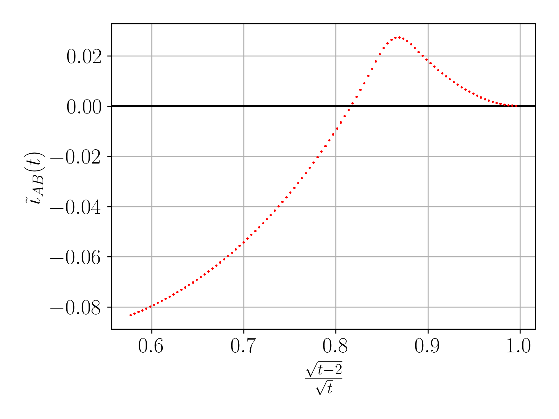
Figure 3: The values of the SDP relaxation of the problem of finding local projective measurements witnessing the non-positivity of the $AB$-Cut-Bell-Wigner operators for the parameterized family of states $\rho_{ABC}(t)$.

As can be seen in the figure, the value of $\tilde{\iota}_{AB}(t)$ is strictly positive when $\frac{\sqrt{t-2}}{\sqrt{t}}\gtrapprox 0.82$. By Eq. (54), this implies that the value of $\iota_{AB}(t)$ is also strictly positive in this region, and consequently that the incompatibility of states in this region are not distribution-witnessable by the $AB$-Cut inflation. The specific choice of $t_{*}$ considered above lies in this region, so $\rho_{ABC}(t_{*})$ is an example of a state that is triangle-incompatible, but for which this incompatibility is not distribution-witnessable.

IV.3 The Compatibility Problem for Mixed States

For the case of pure three-qubit states considered above, all product and biseparable states were shown to be triangle-compatible in Section IV.1. However, we have already seen that the analogous statement is not true for mixed states: recall from above that the separable states $\rho^{({\rm GHZdistn})}$ and $\rho^{({\rm Wdistn})}$ that encode the classical distributions $P^{({\rm GHZ})}$ and $P^{({\rm W})}$ respectively, are triangle-incompatible. In general, any state $\rho^{({\rm distn})}$ that encodes a classical distribution in this way is triangle-incompatible if and only if the corresponding distribution is triangle-incompatible.

Since characterizing the precise set of probability distributions on three binary variables that are compatible with the triangle scenario in a quantum causal model is computationally challenging (for every non-fanout inflation it involves an infinite hierarchy of semi-definite programs [17]), a full classification of the three-qubit mixed states that are compatible with the triangle scenario is at least as difficult.

Nonetheless, one can use the technique described here to easily derive witnesses of incompatibility for mixed quantum states.

Some of the results of Ref. [35] also provide a means for witnessing triangle-incompatibility, using ideas from the inflation technique. In fact, Ref. [35] sought to witness incompatibility for a slightly different network: the triangle supplemented by three-way shared randomness. But if one cannot realize a state with the shared randomness, then one clearly cannot realize that state without it, so any incompatibility in the former case implies triangle-incompatibility. Specifically, the witnesses considered were based on the fidelities between $\rho_{ABC}$ and the GHZ and W states (defined, respectively, in Eqs. (43) and(44)). One witnesses the incompatibility of $\rho_{ABC}$ with the shared-randomness-supplemented triangle (and hence with the triangle) whenever these fidelities satisfy

$$\braket{GHZ|\rho_{ABC}|GHZ}\geq\frac{1+\sqrt{3}}{4}\simeq 0.6803,$$ (55)

$$\braket{W|\rho_{ABC}|W}\geq 0.7602,$$ (56)

Our technique can witness triangle-incompatibilities that are not detected by the fidelity witnesses of Ref. [35]. This is the case even if we limit ourselves to the lowest level of the hierarchy of nonfanout inflations (i.e., we just consider the Cut inflation), while the bounds on the fidelities just mentioned are derived by considering higher levels of this hierarchy.

Consider the following mixed state:

$$\omega_{ABC}=0.3\ket{\psi_{1}}\!\!\bra{\psi_{1}}+0.7\ket{0\!+\!+}\!\!\bra{0\!+\!+}$$ (57)

where

$$\ket{\psi_{1}}:=0.9\ket{000}+\sqrt{0.19/2}\ket{101}+\sqrt{0.19/2}\ket{110}.$$ (58)

By a straightforward calculation, one can compute the operator $I_{AB}(\omega_{ABC})$ and determine that its eigenvalues are

$$\{0.78839,0.195995,0.0351218,-0.0195072\},$$ (59)

each with multiplicity $2$. The occurrence of the negative eigenvalue clearly indicates the non-positivity of $I_{AB}(\omega_{ABC})$ and hence the triangle-incompatibility of $\omega_{ABC}$.

On the other hand, the fidelities between $\omega_{ABC}$ and the GHZ and W states are

$$\braket{GHZ|\omega_{ABC}|GHZ}=0.209,$$ (60)

$$\braket{W|\omega_{ABC}|W}=0.233333,$$ (61)

and hence these fidelities do not satisfy the condition in Eq. (55) for witnessing incompatibility.

IV.3.1 Probing triangle-incompatibility of one-parameter families of mixed states

We saw for the case of pure three-qubit states that the boundary between compatible and incompatible states coincided exactly with the boundary between biseparable states and not biseparable states. We also saw above that in the case of mixed states, the compatibility-incompatibility boundary is far less clear as there are separable states that are triangle-incompatible.

One method to probe this boundary further in the case of mixed states is by adding noise to a pure state and seeing how the positivity of a triangle-incompatibility witness behaves. Here, we consider a simple one parameter noise model that adds white noise to a given pure state. Explicitly, for a given pure three-qubit state $\ket{\Psi}$, we consider the family indexed by $p\in[0,1]$ defined by

$$\hat{\rho}(\ket{\Psi},p):=p\ket{\Psi}\!\!\bra{\Psi}+\frac{1-p}{8}\mathbb{1}_{ABC}$$ (62)

where $\mathbb{1}_{ABC}$ is the identity on $\mathcal{H}_{A}\otimes\mathcal{H}_{B}\otimes\mathcal{H}_{C}$. For any $p<1$, $\hat{\rho}(\ket{\Psi},p)$ is a full rank state. We have the following result:

Proposition 2.

For any $\ket{\Psi}$, there exists a $q\in[3-2\sqrt{2},1)$ such that for all $0\leq p\leq q$, $\hat{\rho}(\ket{\Psi},p)$ is not demonstrably triangle-incompatible using the triangle-incompatibility witnesses of Eq. (36), i.e., $I_{xy}(\hat{\rho}(\ket{\Psi},p))\geq 0$ for each $xy\in\{AB,AC,BC\}$.

The proof is given in Section A.5. The result holds for any choice of the pure state $\ket{\Psi}$ appearing in Eq. (62), which naturally includes all $\ket{\Psi}$ that are not biseparable (which we know to be demonstrably triangle-incompatible using one of the witnesses $I_{xy}$ for $xy\in\{AB,AC,BC\}$).

In general, the value of $q$ will be higher than $3-2\sqrt{2}$. For instance, if we take $\ket{\Psi}=\ket{GHZ}=\frac{1}{\sqrt{2}}(\ket{000}+\ket{111})$, making $\hat{\rho}$ a generalized three-qubit Werner state [36, 37], we get that $q=\frac{1}{2}$. In this case, all the witnesses $I_{xy}(\hat{\rho}(\ket{GHZ},p))$ are non-positive for $p>\frac{1}{2}$, thereby witnessing the triangle-incompatibility of $\hat{\rho}(\ket{GHZ},p)$ for these values (see Section A.5).

Does this tell us anything regarding the relation (or lack thereof) between the entangled-separable boundary and the boundary between triangle-compatible and triangle-incompatible states? As demonstrated in Ref. [36], the state $\hat{\rho}(\ket{GHZ},p)$ is entangled for any $p\gtrapprox 0.69554$ (as witnessed by the positivity of the three-tangle for those values). It follows that the entanglement boundary and triangle-incompatibility boundary are indeed distinct for this simple class of states: for $\frac{1}{2}<p<0.6955$, the states $\hat{\rho}(\ket{GHZ},p)$ are triangle-incompatible but not entangled. Section A.5 includes some details of the calculations of these $q$-values, also for the case where $\ket{\Psi}=\ket{W}=\frac{1}{\sqrt{3}}(\ket{001}+\ket{010}+\ket{100})$ which produces $q\approx 0.627$.

An alternative family of Werner-like three-qubit mixed states was studied in Ref. [38]. This single-parameter family is defined by

$$\rho^{(3,c)} :=\frac{1}{8}\mathbb{1}_{ABC}+\sum_{k=X,Y,Z}\frac{1}{24}\mathbb{1}_{A}\otimes\sigma_{B}^{(k)}\otimes\sigma_{C}^{(k)}$$

$$\quad-\frac{c}{16}\left(\sigma_{A}^{(k)}\otimes\mathbb{1}_{B}\otimes\sigma_{C}^{(k)}+\sigma_{A}^{(k)}\otimes\sigma_{B}^{(k)}\otimes\mathbb{1}_{C}\right)$$ (63)

where $c$ is a real parameter, the $\sigma^{(k)}$ denote the Pauli matrices, and the subscripts indicate the subsystems they act upon. This family is interesting since it permits a local hidden variable model for projective measurements whenever $c\leq 1$ (c.f. [Thm 2, 38]) and is not biseparable for $c>\frac{1}{3}(\sqrt{13}-1)$. If $c=0$, one observes that the $\rho^{(3,c)}$ factorizes across the $A|BC$ partition (and moreover is maximally mixed on the $A$ subsystem). By analogous arguments to the provided for biseparable pure states, this state can be seen to be triangle-compatible. It turns out that this state is the only member of the above family that is; all the rest are triangle-incompatible.

Proposition 3.

The state $\rho^{(3,c)}$ is triangle-incompatible if and only if $c\neq 0$.

The proof is given in Section A.6. For this class of states then, it appears that the incompatibility-compatibility boundary has less to do with the separability than the factorizability of the state in question.

In sum, apart from providing further evidence that the triangle-incompatibility witnesses introduced above are broadly applicable to mixed states, the results presented in this subsection point to the greater nuance involved in attempting to categorize the triangle-compatibility of mixed as opposed to pure states.

V Visible Nodes Beyond Qubits

The operator inequality in (22) was established by Hall for any finite dimensional Hilbert space. Thus, the methodology of analyzing the positivity of the associated triangle-incompatibility witnesses remains valid in the cases where the visible nodes are not qubits. In this section, we provide a couple of examples of states on higher-dimensional systems that are triangle-incompatible.

V.1 Two Qubits and One Ququart, Pure States

Our first higher-dimensional example is to consider pure states where $\mathcal{H}_{A}\cong\mathcal{H}_{B}\cong\mathbb{C}^{2}$ and $\mathcal{H}_{C}\cong\mathbb{C}^{4}$. Unlike the three-qubit case, it is readily seen that for such a choice of systems, there are triangle-compatible states beyond those that factorize across a bipartition. It suffices to note that the ququart can be conceptualized as a pair of qubits, say $C^{(1)}$ and $C^{(2)}$, and it is clear that in the triangle scenario one can prepare an entangled state on $AC^{(1)}$ and an entangled state on $BC^{(2)}$.

This of course does not imply that any pure qubit-qubit-ququart state can be prepared. For example, since a qubit can be isometrically embedded in a ququart, there are qubit-qubit-ququart states that are local isometry-equivalent to the three-qubit pure states that are triangle-incompatible, and hence are themselves triangle-incompatible. However, there exist qubit-qubit-ququart states that do not reduce to three-qubit states and we now demonstrate that we can use the triangle-incompatibility witnesses presented above to prove the triangle-incompatibility of some such states, including those exhibiting GHZ-like entanglement.

To consider pure states on this qubit-qubit-ququart system, it is possible to use the higher-dimensional generalised Schmidt decomposition given in Ref. [39]. A pure state $\ket{\Psi}\in\mathcal{H}_{A}\otimes\mathcal{H}_{B}\otimes\mathcal{H}_{C}$ can be written as

$$\ket{\Psi} =\alpha_{0}e^{i\phi_{0}}\ket{000}+\alpha_{1}\ket{011}+\alpha_{2}\ket{101}+\alpha_{3}e^{i\phi_{1}}\ket{102}$$

$$\quad+\alpha_{4}\ket{110}+\alpha_{5}\ket{111}+\alpha_{6}\ket{112}+\alpha_{7}\ket{113}$$ (64)

where $\alpha_{l}\in\mathbb{R}_{\geq 0}$, $\sum_{l}\alpha_{l}^{2}=1$ and $\phi_{r}\in[0,2\pi)$ (see Appendix B for a summary of how this form is obtained from the general form in [39]). We then have the following:

Proposition 1.

If $\rho_{ABC}=\ket{\Psi}\!\!\bra{\Psi}$ where

$$\ket{\Psi}=\alpha_{0}e^{i\phi_{0}}\ket{000}+\alpha_{4}\ket{110}+\alpha_{5}\ket{111}+\alpha_{6}\ket{112}+\alpha_{7}\ket{113}$$ (65)

with $0<\alpha_{0}^{2}+\alpha_{4}^{2}<1$ (i.e. at least one of $\alpha_{5}$, $\alpha_{6}$ and $\alpha_{7}$ is non-zero), then $\rho_{ABC}$ is triangle-incompatible and this incompatibility is distribution-witnessable.

The proof is given in Section A.7 and proceeds by demonstrating that $I_{AC}(\ket{\Psi}\!\!\bra{\Psi})$ is not positive for the relevant values of the $\alpha$ parameters. It should be noted that the above result is consistent with known results establishing the impossibility of generating qudit graph states, such as the GHZ state, in networks with bipartite sources (see e.g., [40]), but extends also to other local-unitary inequivalent states that exhibit GHZ-like entanglement.

V.2 Three Qutrits, Mixed States

For the case of three qubits, we saw a number of distinctions between pure and mixed states vis-a-vis triangle-compatibility. Here, we give one final example in a similar vein for the case of three qutrits. In this example, we consider a pure three-qutrit state and a mixed three-qutrit state which have the same level of multipartite entanglement as quantified by the generalized geometric measure of entanglement (GGM) [41, 42, 43], where for the former, triangle-incompatibility can be demonstrated using the triangle-incompatibility witness while for the latter it cannot.

In Ref. [44], the GGM was calculated for a number of mixed states exhibiting certain symmetries. In particular, these mixed states were obtained from specific pure states via a certain choice of twirling operation, allowing the GGM of the former to be related to that of the latter. One example of this pure state - mixed state pairing is given by

$$\ket{\Psi_{3,3}^{(3)}}:=\sqrt{p_{0}}\ket{\Psi_{0}}+\sqrt{p_{1}}\ket{\Psi_{1}}+\sqrt{1-p_{0}-p_{1}}\ket{\Psi_{2}},$$ (66)

$$\rho_{3,3}^{(3)}:=p_{0}\ket{\Psi_{0}}\!\!\bra{\Psi_{0}}+p_{1}\ket{\Psi_{1}}\!\!\bra{\Psi_{1}}+(1-p_{0}-p_{1})\ket{\Psi_{2}}\!\!\bra{\Psi_{2}},$$ (67)

where $p_{0},p_{1},p_{0}+p_{1}\in[0,1]$ and where $\ket{\Psi_{i}}$ are the three-qutrit states defined to be an equal superposition of computational basis states $\ket{xyz}$ such that $x+y+z=i\bmod 3$, that is,

$$\ket{\Psi_{0}}:=\frac{1}{3} \left(\ket{000}+\ket{111}+\ket{222}\right.$$

$$\left.\ket{012}+\ket{021}+\ket{102}\right.$$

$$\left.\ket{120}+\ket{201}+\ket{210}\right),$$ (68)

$$\ket{\Psi_{1}}:=\frac{1}{3} \left(\ket{001}+\ket{010}+\ket{100}\right.$$

$$\left.\ket{022}+\ket{202}+\ket{220}\right.$$

$$\left.\ket{112}+\ket{121}+\ket{211}\right),$$ (69)

$$\ket{\Psi_{2}}:=\frac{1}{3} \left(\ket{011}+\ket{101}+\ket{110}\right.$$

$$\left.\ket{002}+\ket{020}+\ket{200}\right.$$

$$\left.\ket{122}+\ket{212}+\ket{221}\right).$$ (70)

Let $Z_{3}$ denote the qutrit analogue of the qubit Pauli-$Z$ operator, i.e., $Z_{3}=\sum_{j=0}^{2}e^{\frac{2\pi ij}{3}}\ket{j}\!\!\bra{j}$. For the twirling operator $\bm{P}:\mathcal{L}(\mathcal{H}_{A}\otimes\mathcal{H}_{B}\otimes\mathcal{H}_{C})\rightarrow\mathcal{L}(\mathcal{H}_{A}\otimes\mathcal{H}_{B}\otimes\mathcal{H}_{C})$ defined via

$$\rho\mapsto\frac{1}{3}\sum_{k=0}^{2}\left(Z_{3}^{k}\otimes Z_{3}^{k}\otimes Z_{3}^{k}\right)\rho(Z_{3}^{k}\otimes Z_{3}^{k}\otimes Z_{3}^{k})^{\dagger}$$ (71)

where $Z_{3}^{k}$ denotes the $k$th power of $Z_{3}$, we have that $\bm{P}(\ket{\Psi_{3,3,}^{(3)}}\!\!\bra{\Psi_{3,3}^{(3)}})=\rho_{3,3}^{(3)}$.

As a consequence of the above relation via $\bm{P}$, the GGM of $\ket{\Psi_{3,3}^{(3)}}$ and that of $\rho_{3,3}^{(3)}$ coincide. However, when it comes to proving the triangle-compatibility of these states by the witness $I_{AB}$, there is a difference between them. It turns out that $I_{AB}(\rho_{3,3}^{(3)})$, $I_{AC}(\rho_{3,3}^{(3)})$, and $I_{BC}(\rho_{3,3}^{(3)})$ have no dependence on $p_{0},p_{1}$ and moreover have eigenvalues $\frac{7}{9}$ with multiplicity $3$, $\frac{4}{9}$ with multiplicity $12$ and $\frac{1}{9}$ also with multiplicity $12$. We can thus not draw any conclusions about the triangle-compatibility of $\rho_{3,3}^{(3)}$ using this method alone.

Conversely, taking e.g., $p_{0}=2p_{1}=0.5$, one finds that $I_{AB}(\ket{\Psi_{3,3}^{(3)}}\!\!\bra{\Psi_{3,3}^{(3)}})$ has an eigenvalue equal to $-0.01348$ and so $\ket{\Psi_{3,3}^{(3)}}$ is triangle-incompatible for these values of $p_{0},p_{1}$. Note that other values of $p_{0},p_{1}$ also exist for which incompatibility can be demonstrated.

VI Discussion

Demonstrating the compatibility of a probability distribution or quantum state with a causal structure is in general a difficult task. In this article we have presented a method for witnessing the incompatibility of quantum states based on a family of quantum marginal constraints (in the form of the operator inequalities of Eq. (23)) in conjunction with the inflation technique. We have furthermore presented an array of results that demonstrate that this method can indeed be used to make progress on problems of causal compatibility.

One of the key benefits of this approach pertains to its scalability. As demonstrated in, e.g., Ref [45], quantum marginal problems admit a semidefinite programming formulation. Accordingly, when using the inflation technique for investigating questions of causal compatibility, one can always consider the corresponding SDP. However, in the cases where a witness can be obtained by a marginal inequality, such as those in Eq. (23), there is a slight advantage in terms of computational complexity as we now describe. Denoting the product of the dimensions of the subsystems involved by $D$, the complexity of the SDP associated to the quantum marginal problem is $\mathcal{O}(D^{\frac{13}{2}})$ [45]. For example, for the marginal problems derived from a choice of inflation of a causal structure with qubit visible nodes, the SDP complexity would be $\mathcal{O}(2^{\frac{13n}{2}})$, where $n$ is the number of visible nodes in the inflation DAG. Alternatively, the complexity of finding the eigendecomposition of a $D\times D$ matrix in practice is typically stated as being $\mathcal{O}(D^{3})$ (improvements to the exponent exist in certain cases). Thus, producing an incompatibility witness corresponding to an inflation DAG with $n$ qubit visible nodes allows us to perform an incompatibility test with complexity $\mathcal{O}(2^{3n})$ or better. This is clearly not an exponential speed-up over the SDP case, but it is a speed-up nonetheless.

As a consequence of this favourable scaling, we believe the method presented here has pragmatic value. As experimental realizations of quantum networks improve (see, e.g., [46, 47, 48]), it will be increasingly important to have practical methods for verifying the structure of such networks. For example, using the methods presented above it may be possible to verify that a tomographically-specified network state could not have been produced in a causal structure representing the desired network, thereby revealing a deficiency in the experimentalist’s account of the set-up. Furthermore, an understanding of whether it is possible to witness incompatibility via a probability distribution arising from local measurements allows for a better appreciation of the requirements for verifying a network structure.

There are also potential benefits of the approach presented here for classical causal inference. Since the quantum compatibility problem subsumes the classical compatibility problem (as every distribution can be expressed as a diagonal density operator), a test for compatibility of quantum states is also a test for compatibility of distributions. Sometimes the more abstract problem leads to progress on the more concrete problem, so it is conceivable that investigations of the sort described here and comparisons of the classical and fully quantum causal inference problems more generally, might ultimately yield dividends for classical causal inference.

The notion of a causal model can be generalized not just from classical theories to quantum, but to any generalized probabilistic theory (GPT) (see e.g., [49]). Boxworld [50], the toy theory of Ref. [51], and real quantum theory[52, 53] are prominent examples. These theories are generally studies as foils to quantum theory, clarifying the meaning of the latter. As such, an interesting problem for future research is to study the causal compatibility problem within generalized probabilistic theories of interest and compare to the quantum case. As emphasized in this article, if one wishes to derive such constraints using the inflation technique, then one must have some constraints coming from the marginal problem to leverage. This, therefore, motivates a study of the marginal problem in various GPTs of interest.

Appendix A Proofs

This appendix contains the proofs of the results presented in the main text.

A.1 Proof of 1

The proof of the following lemma uses properties of the max-divergence, some of which are provided below. The reader is referred to the relevant sections of e.g., [54, 55] for further details.

Let $\widetilde{D}_{\alpha}(\cdot\|\cdot)$ denote the sandwiched Rényi relative entropy where $\alpha\in(0,1)\cup(1,\infty)$. The relevance of this relative entropy for the purposes of 1 is via its connection to the max relative entropy defined via

$$D_{\max}(\rho\|\sigma)=\log_{2}\inf\{\lambda\in\mathbb{R}:\rho\leq\lambda\sigma\}.$$ (72)

The connection between the sandwiched Rényi relative entropy and the max relative entropy is established through the following proposition:

Proposition 1 ([54]).

The sandwiched Rényi relative entropy converges to the max relative entropy in the limit $\alpha\rightarrow\infty$

$$\lim_{\alpha\rightarrow\infty}\widetilde{D}_{\alpha}(\rho\|\sigma)=D_{\max}(\rho\|\sigma).$$ (73)

As a consequence of the above proposition, the max relative entropy shares a number of properties with the sandwiched Rényi relative entropies, including those stated below:

Proposition 2 ([54]).

The sandwiched Rényi relative entropy $\widetilde{D}_{\alpha}$ satisfies the following properties for every states $\rho$ and positive semi-definite operator $\sigma$ for $\alpha\in[1/2,1)\cup(1,\infty)$.

1. If $\operatorname{Tr}[\sigma]\leq\operatorname{Tr}[\rho]=1$, then $\widetilde{D}_{\alpha}(\rho\|\sigma)\geq 0$.

2. Faithfulness: If $\operatorname{Tr}[\sigma]\leq 1$, we have that $\widetilde{D}_{\alpha}(\rho\|\sigma)=0$ if and only if $\rho=\sigma$.

3. If $\rho\leq\sigma$, then $\widetilde{D}_{\alpha}(\rho\|\sigma)\leq 0$.

4. For every PSD operator $\sigma^{\prime}$ such that $\sigma^{\prime}\geq\sigma$, we have $\widetilde{D}_{\alpha}(\rho\|\sigma)\geq\widetilde{D}_{\alpha}(\rho\|\sigma^{\prime})$.

The first three items above are of the most relevance for the proof the lemma:

Proof of 1.

Let $\rho_{xy}$ be such that $\rho_{xy}\neq\rho_{x}\otimes\rho_{y}$. Suppose for a contradiction that $\rho_{xy}\leq\rho_{x}\otimes\rho_{y}$. From the consequences of 1, we know that the max relative entropy satisfies Items 1, 2 and 3 from 2. Since $\rho_{xy}$ and $\rho_{x}\otimes\rho_{y}$ are both quantum states and hence of unit trace, from Item 1 we can conclude that $D_{\max}(\rho_{xy}\|\rho_{x}\otimes\rho_{y})\geq 0$. From the assumption that $\rho_{x,y}\neq\rho_{x}\otimes\rho_{y}$, we can conclude from Item 2 that $D_{\max}(\rho_{xy}\|\rho_{x}\otimes\rho_{y})\neq 0$ and hence must be strictly positive. However, the assumption that $\rho_{xy}\leq\rho_{x}\otimes\rho_{y}$ and Item 3 imply that $D_{\max}(\rho_{xy}\|\rho_{x}\otimes\rho_{y})\leq 0$, forming the desired contradiction. The conclusion that $\rho_{xy}\leq\rho_{x}\otimes\rho_{y}$ implies that $D_{\max}(\rho_{xy}\|\rho_{x}\otimes\rho_{y})\leq 0$ can be seen directly from Eq. 72 since $\rho_{xy}\leq\rho_{x}\otimes\rho_{y}$ is equivalent to $\rho_{xy}\leq\lambda\rho_{x}\otimes\rho_{y}$ for $\lambda=1$. It follows that

$$\inf\{\lambda\in\mathbb{R}:\rho_{xy}\leq\lambda\rho_{x}\otimes\rho_{y}\}\leq 1$$ (74)

and so taking the logarithm produces a non-positive value for $D_{\max}(\rho_{xy}\|\rho_{x}\otimes\rho_{y})$. ∎

A.2 Distribution-Witnessability of W-state

Here we demonstrate that, unlike the state $\rho^{({\rm Wdistn})}$ that encodes the $W$-distribution, the triangle-incompatibility of the state $\rho^{({\rm W})}:=\ket{{\rm W}}\!\!\bra{{\rm W}}$ with $\ket{{\rm W}}=\frac{1}{\sqrt{3}}(\ket{001}+\ket{010}+\ket{100})$ is distribution-witnessable using the cut-inflation.

Recall that we can write the triangle-incompatibility witness $I_{AB}$ as

$$I_{AB}(\rho^{({\rm W})})=\Delta(\{\rho_{{\bm{X}}}^{({\rm W})}:{\bm{X}}\in 2^{{\bm{V}}}\setminus{\bm{V}}\})+(\rho_{A}^{({\rm W})}\otimes\rho_{B}^{({\rm W})}-\rho_{AB}^{({\rm W})})\otimes I_{C}$$ (75)

where ${\bm{V}}=\{A,B,C\}$. We have that

$$\Delta(\{\rho_{{\bm{X}}}^{({\rm W})}:{\bm{X}}\in 2^{{\bm{V}}}\setminus{\bm{V}}\})=\begin{bmatrix}0&0&0&0&0&0&0&0\\ 0&\frac{1}{3}&\frac{1}{3}&0&\frac{1}{3}&0&0&0\\ 0&\frac{1}{3}&\frac{1}{3}&0&\frac{1}{3}&0&0&0\\ 0&0&0&\frac{1}{3}&0&\frac{1}{3}&\frac{1}{3}&0\\ 0&\frac{1}{3}&\frac{1}{3}&0&\frac{1}{3}&0&0&0\\ 0&0&0&\frac{1}{3}&0&\frac{1}{3}&\frac{1}{3}&0\\ 0&0&0&\frac{1}{3}&0&\frac{1}{3}&\frac{1}{3}&0\\ 0&0&0&0&0&0&0&0\end{bmatrix}$$ (76)

and

$$\rho_{A}^{({\rm W})}\otimes\rho_{B}^{({\rm W})}-\rho_{AB}^{({\rm W})}=\begin{bmatrix}\frac{1}{9}&0&0&0\\ 0&-\frac{1}{9}&-\frac{1}{3}&0\\ 0&-\frac{1}{3}&-\frac{1}{9}&0\\ 0&0&0&\frac{1}{9}\end{bmatrix}.$$ (77)

Consequently, we have that

$$\bra{++-}I_{AB}(\rho^{({\rm W})})\ket{++-} =\bra{++-}\Delta(\{\rho_{{\bm{X}}}^{({\rm W})}:{\bm{X}}\in 2^{{\bm{V}}}\setminus{\bm{V}}\})\ket{++-}+\bra{++}\rho_{A}^{({\rm W})}\otimes\rho_{B}^{({\rm W})}-\rho_{AB}^{({\rm W})}\ket{++}$$ (78)

$$=\frac{1}{12}-\frac{1}{6}$$ (79)

and so the probability distribution that results from measuring each subsystem of $\rho^{(W)}$ in the $X$-basis is triangle-incompatible.

A.3 Proof of 1

Prior to proving the theorem, it is convenient to show the following lemma:

Lemma 2.

If $\ket{\omega_{AB}}\in\mathcal{H}_{A}\otimes\mathcal{H}_{B}$, $\ket{\omega_{AC}}\in\mathcal{H}_{A}\otimes\mathcal{H}_{C}$ and $\ket{\omega_{BC}}\in\mathcal{H}_{B}\otimes\mathcal{H}_{C}$ are non-zero, then the sets

$$\{\ket{\omega_{AB}}\otimes\ket{0}_{C},\ket{\omega_{AB}}\otimes\ket{1}_{C},\ket{\omega_{AC}}\otimes\ket{0}_{B},\ket{\omega_{AC}}\otimes\ket{1}_{B}\},$$ (80)

$$\{\ket{\omega_{AB}}\otimes\ket{0}_{C},\ket{\omega_{AB}}\otimes\ket{1}_{C},\ket{\omega_{BC}}\otimes\ket{0}_{A},\ket{\omega_{BC}}\otimes\ket{1}_{A}\},$$ (81)

$$\{\ket{\omega_{AC}}\otimes\ket{0}_{B},\ket{\omega_{AC}}\otimes\ket{1}_{B},\ket{\omega_{BC}}\otimes\ket{0}_{A},\ket{\omega_{BC}}\otimes\ket{1}_{A}\},$$ (82)

each contain at least three linearly independent vectors.

Proof.

We demonstrate the proof for Eq. 80; the proof for the other sets are analogous. Let $\ket{\omega_{AB}}=[a,b,c,d]^{\top}$ and $\ket{\omega_{AC}}=[a^{\prime},b^{\prime},c^{\prime},d^{\prime}]^{\top}$ where at least one of $a,b,c,d$ and at least one of $a^{\prime},b^{\prime},c^{\prime},d^{\prime}$ are non-zero by assumption. Suppose that

$$\ket{\omega_{AC}}\otimes\ket{0}_{B} =\alpha\ket{\omega_{AB}}\otimes\ket{0}_{C}+\beta\ket{\omega_{AB}}\otimes\ket{1}_{C},$$ (83)

$$\ket{\omega_{AC}}\otimes\ket{1}_{B} =\gamma\ket{\omega_{AB}}\otimes\ket{0}_{C}+\delta\ket{\omega_{AB}}\otimes\ket{1}_{C},$$ (84)

where neither $\alpha$ and $\beta$ nor $\gamma$ and $\delta$ are both-zero. The first equation requires that $b$ and $d$ both be $0$, while the second equation requires that both $a$ and $c$ be $0$, forming a contradiction. It follows that at least one of $\ket{\omega_{AC}}\otimes\ket{0}_{B}$ and $\ket{\omega_{AC}}\otimes\ket{1}_{B}$ is linearly independent of $\ket{\omega_{AB}}\otimes\ket{0}_{C}$ and $\ket{\omega_{AB}}\otimes\ket{1}_{C}$. ∎

Let ${\bf V}:=\{A,B,C\}$. A further useful fact for the proof of 1 arises from the proof of Theorem $3.2$ in [25]: for $\mathcal{H}_{A}\cong\mathcal{H}_{B}\cong\mathcal{H}_{C}\cong\mathbb{C}^{2}$, we have that

$$\Delta(\{\rho_{{\bf X}}:{\bf X}\in 2^{{\bf V}}\!\setminus\!{\bf V}\})=\rho+\tau^{-1}\rho\tau$$ (85)

where $\tau$ is the three qubit antiunitary defined by its action on pure states via

$$\tau\sum_{i,j,k}\alpha_{i,j,k}\ket{ijk}=\sum_{i,j,k}(-1)^{i+j+k}\alpha_{ijk}^{*}\ket{\overline{i}\overline{j}\overline{k}}$$ (86)

with $i,j,k\in\{0,1\}$ and $\overline{x}:=1-x$.

Proof of 1.

Suppose $\rho_{ABC}=\ket{\Psi}\!\!\bra{\Psi}$ where $\ket{\Psi}$ is genuinely tripartite entangled, meaning that each of the two-party marginals satisfies $\rho_{xy}\neq\rho_{x}\otimes\rho_{y}$. As a consequence of 1, $\rho_{A}\otimes\rho_{B}-\rho_{AB}$, $\rho_{A}\otimes\rho_{C}-\rho_{AC}$ and $\rho_{B}\otimes\rho_{C}-\rho_{BC}$ are not positive semi-definite and hence have a eigenvector with a negative eigenvalue. Let $\omega_{xy}\in\mathcal{H}_{x}\otimes\mathcal{H}_{y}$ denote an eigenvector of $\rho_{x}\otimes\rho_{y}-\rho_{xy}$ with negative eigenvalue, for $x\neq y\in\{A,B,C\}$. As a consequence of 2, we have that

$$\dim(\operatorname{supp}(\nu_{AB}^{-}\otimes\mathbb{1}_{C})\cup\operatorname{supp}(\nu_{AC}^{-}\otimes\mathbb{1}_{B})\cup\operatorname{supp}(\nu_{BC}^{-}\otimes\mathbb{1}_{A}))\geq 3.$$ (87)

From Eq. 85 and that $\rho_{ABC}$ is pure, we get that $\dim(\operatorname{supp}(\Delta(\{\rho_{{\bf X}}:{\bf X}\in 2^{{\bf V}}\!\setminus\!{\bf V}\})))=2$. It follows that there exists a $\ket{\Phi}\in\operatorname{supp}(\nu_{xy}^{-}\otimes\mathbb{1}_{z})\cap\ker(\Delta(\{\rho_{{\bf X}}:{\bf X}\in 2^{{\bf V}}\!\setminus\!{\bf V}\}))$ for some $x,y,z\in\{A,B,C\}$ with $x\neq y\neq z\neq x$, and so the result follows from 2. ∎

A.4 Proof of 1

1 presented in the main text establishes that there exist states whose triangle-incompatibility is not distribution-witnessable. The proof of this proposition makes use of a one-parameter family of pure states:

$$\ket{\Psi(t)}=\frac{\sqrt{t-2}}{\sqrt{t}}\ket{100}+\frac{1}{\sqrt{t}}\ket{001}+\frac{1}{\sqrt{t}}\ket{010},$$ (88)

where $t$ is a real parameter in the interval $[3,\infty)$. These are categorized as ‘tri-Bell’ states according to the classification of Ref. [56]. Note that the boundary of this family, at $t=3$, is the W state of Eq. (44). We will use the notation $\rho_{ABC}(t)$ for the member of this family for a given $t$.

Since every element of this family of states (for finite $t$) fails to factorize across any bipartition, by Theorem 1, they are all incompatible with the triangle scenario. Furthermore, this incompatibility can be demonstrated using the triangle-incompatibility witness $I_{AB}$, as we will now see.

For $\rho_{ABC}(t)$, the eigenvalues of $I_{AB}(\rho_{ABC}(t))$ are

$$\left\{\frac{1}{t^{2}}(t-2),\frac{r_{1}}{t^{2}},\frac{r_{2}}{t^{2}},\frac{r_{3}}{t^{2}}\right\}$$ (89)

each with multiplicity $2$, where $r_{1},r_{2},r_{3}$ are the roots of the cubic polynomial

$$f(x)=x^{3} +(-t^{2}+t-2)x^{2}+(-4+8t-5t^{2}+t^{3})x+(8-20t+14t^{2}-5t^{3}+t^{4}).$$ (90)

For a given $t\geq 3$, the demonstration of a negative value for $r_{1}$, $r_{2}$ or $r_{3}$ suffices to prove that $\rho_{ABC}(t)$ is triangle-incompatible. Since $I_{AB}(\rho_{ABC}(t))$ is Hermitian for all $t$, it must be that $r_{1},r_{2},r_{3}\in\mathbb{R}$. Via Vieta’s formula [57] (see also [58]), we get that

$$r_{1}r_{2}r_{3}=-(8-20t+14t^{2}-5t^{3}+t^{4}).$$ (91)

As the quartic polynomial inside the brackets on the right-hand side is strictly positive for $t>2$, it follows that $r_{1}r_{2}r_{3}$ is strictly negative, indicating at least one negative root. Thus $\rho_{ABC}(t)$ is triangle-incompatible for the range of values of $t$ that we consider (i.e. $t\geq 3$). Any normalized eigenvector corresponding to a negative eigenvalue is thus a state that witnesses this incompatibility.

The fact that there exist values of $t$ such that incompatibility of $\rho_{ABC}(t)$ is not distribution-witnessable was presented in the main text. To show that $\rho_{ABC}(t)$ for certain $t$ is not distribution-witnessable using the AB-Cut inflation is equivalent to demonstrating that the quantity

$$\iota_{AB}(\rho_{ABC}(t)) :=\min_{\ket{\phi_{A}},\ket{\phi_{B}},\ket{\phi_{C}}}\bra{\phi_{A}\phi_{B}\phi_{C}}I_{AB}(\rho_{ABC}(t))\ket{\phi_{A}\phi_{B}\phi_{C}}$$ (92)

is non-negative. To do so, we consider a relaxation of the above non-convex optimization to a convex one, namely

$$\tilde{\iota}_{AB}(\rho_{ABC}(t)) :=\min_{\varrho_{ABC}\in S}\operatorname{Tr}[\varrho_{ABC}I_{AB}(\rho_{ABC}(t))],$$ (93)

where $S$ denotes the set of all three-qubit states with positive partial transposes over each subsystem, that is:

$$S:=\{\varrho_{ABC}:\varrho_{ABC}^{\top_{A}}\geq 0,\varrho_{ABC}^{\top_{B}}\geq 0,\varrho_{ABC}^{\top_{C}}\geq 0\}.$$ (94)

This set $S$ contains the set of pure product states, meaning that $\iota_{ABC}(t)$ is guaranteed to be lower bounded by $\tilde{\iota}_{ABC}(t)$. As discussed in the main text, the latter quantity is indeed non-negative for e.g., $t\geq 7$.

A.5 Proof of 2

Proof of 2.

Let us write $\rho_{ABC}=\ket{\Psi}\!\!\bra{\Psi}$ so $\hat{\rho}(\ket{\Psi},p)=p\rho_{ABC}+\frac{1-p}{8}\mathbb{1}_{ABC}$. For convenience, we will at times write $\hat{\rho}$ for $\hat{\rho}(\ket{\Psi},p)$. By linearity, we see that

$$\Delta(\{\hat{\rho}_{{\bf X}}:{\bf X}\in 2^{{\bf V}}\!\setminus\!{\bf V}\})=p\Delta(\{\rho_{{\bf X}}:{\bf X}\in 2^{{\bf V}}\!\setminus\!{\bf V}\})+(1-p)\Delta\left(\left\{\frac{\mathbb{1}_{{\bf X}}}{2^{|{\bf X}|}}:{\bf X}\in 2^{{\bf V}}\!\setminus\!{\bf V}\right\}\right)$$ (95)

Furthermore, recalling Eq. 28, we have that $\Delta\left(\left\{\frac{\mathbb{1}_{{\bf X}}}{2^{|{\bf X}|}}:{\bf X}\in 2^{{\bf V}}\!\setminus\!{\bf V}\right\}\right)=\frac{1}{4}\mathbb{1}_{ABC}$. We demonstrate that there exists a $q\in[3-2\sqrt{2},1)$ such that $I_{AB}(\hat{\rho}(\ket{\Psi},p))\geq 0$ for all $0\leq p\leq q$; the proofs for the other triangle-incompatibility witnesses proceed analogously, and the result is obtained by taking the minimal value of $q$ for the three cases.

Since

$$\hat{\rho}_{A}\otimes\hat{\rho}_{B} =(p\rho_{A}+\frac{1-p}{2}\mathbb{1}_{A})\otimes(p\rho_{B}+\frac{1-p}{2}\mathbb{1}_{B})$$ (96)

$$=p^{2}\rho_{A}\otimes\rho_{B}+\frac{p(1-p)}{2}\rho_{A}\otimes\mathbb{1}_{B}+\frac{p(1-p)}{2}\mathbb{1}_{A}\otimes\rho_{B}+\frac{(1-p)^{2}}{4}\mathbb{1}_{AB},$$ (97)

$$\hat{\rho}_{AB} =p\rho_{AB}+\frac{(1-p)}{4}\mathbb{1}_{AB},$$ (98)

and $I_{AB}(\hat{\rho})=\Delta(\{\hat{\rho}_{{\bf X}}:{\bf X}\in 2^{{\bf V}}\!\setminus\!{\bf V}\})+\hat{\rho}_{A}\otimes\hat{\rho}_{B}-\hat{\rho}_{AB}$, we get that

$$I_{AB}(\hat{\rho}) =p\Delta(\{\rho_{{\bf X}}:{\bf X}\in 2^{{\bf V}}\!\setminus\!{\bf V}\})+\frac{1-p}{4}\mathbb{1}_{ABC}+p^{2}\rho_{A}\otimes\rho_{B}\otimes\mathbb{1}_{C}+\frac{p(1-p)}{2}\rho_{A}\otimes\mathbb{1}_{BC}$$

$$\quad+\frac{p(1-p)}{2}\mathbb{1}_{AC}\otimes\rho_{B}+\frac{(1-p)^{2}}{4}\mathbb{1}_{ABC}-p\rho_{AB}\otimes\mathbb{1}_{C}-\frac{(1-p)}{4}\mathbb{1}_{ABC}$$ (99)

$$=p\Delta(\{\rho_{{\bf X}}:{\bf X}\in 2^{{\bf V}}\!\setminus\!{\bf V}\})+p^{2}\rho_{A}\otimes\rho_{B}\otimes\mathbb{1}_{C}+\frac{p(1-p)}{2}\rho_{A}\otimes\mathbb{1}_{BC}+\frac{p(1-p)}{2}\mathbb{1}_{AC}\otimes\rho_{B}$$

$$\quad+\frac{(1-p)^{2}}{4}\mathbb{1}_{ABC}-p\rho_{AB}\otimes\mathbb{1}_{C}.$$ (100)

Noting that a sufficient condition for $A-B\geq 0$ for $A$ and $B$ positive semidefinite matrices is that the maximal eigenvalue of $B$ is less than or equal to the minimal eigenvalue of $A$, we see that $\frac{(1-p)^{2}}{4}\mathbb{1}_{ABC}-p\rho_{AB}\otimes\mathbb{1}_{C}\geq 0$ is guaranteed at least when $\frac{1}{4}(1-p)^{2}-p\geq 0$, i.e. for $0\leq p\leq 3-2\sqrt{2}$. It follows that $I_{AB}(\hat{\rho})$ is guaranteed to be positive semidefinite at least for $0\leq p\leq q:=3-2\sqrt{2}$. The same reasoning holds for $I_{AC}$ and $I_{BC}$ with the same value of $q$. ∎

The above proof establishes a lower bound for $q$ that is generally not tight for a given pure state $\ket{\Psi}$. For $\hat{\rho}(\ket{GHZ},p)$, the eigenvalues of $I_{xy}(\hat{\rho})$ are the same for all $xy\in\{AB,AC,BC\}$ and are given by $\frac{1}{4}\{1,1\pm 2p\}$, where the first has multiplicity $4$ and the others multiplicity $2$. Thus, for $p\leq\frac{1}{2}$, the $I_{xy}(\hat{\rho})$ are all positive.

For $\ket{\rho}(\ket{W},p)$, the eigenvalues of $I_{xy}(\hat{\rho})$ are the same for all $xy\in\{AB,AC,BC\}$ and are given by

$$\frac{1}{36}\left\{9-p^{2},9-6p+p^{2},9+3p\pm\sqrt{297p^{2}+6p^{3}+p^{4}}\right\}$$ (101)

each with multiplicity $2$. These eigenvalues are all positive whenever $9+3p\geq\sqrt{297p^{2}+6p^{3}+p^{4}}$, which occurs for $p\lessapprox 0.627$.

A.6 Proof of 3

Any three-qubit mixed state can be written as

$$\rho_{ABC}=\frac{1}{8}\mathbb{1}_{ABC}+\sum_{i,j,k=X,Y,Z}a_{i}\sigma_{A}^{i}+b_{j}\sigma_{B}^{j}+c_{k}\sigma_{C}^{k}+d_{ij}\sigma_{A}^{i}\otimes\sigma_{B}^{j}+e_{ik}\sigma_{A}^{i}\otimes\sigma_{C}^{k}+f_{jk}\sigma_{B}^{j}\otimes\sigma_{C}^{k}+g_{ijk}\sigma_{A}^{i}\otimes\sigma_{B}^{j}\otimes\sigma_{C}^{k}$$ (102)

where the $\sigma^{l}$ for $l=X,Y,Z$ denote the Pauli operators and where all the coefficients are real. Each term in the above expression is to be understood as an operator $\mathcal{H}_{A}\otimes\mathcal{H}_{B}\otimes\mathcal{H}_{C}$ - identity operators have been omitted for brevity.

Substituting the expression for $\rho_{ABC}$ into Eq. 33 and the corresponding equations for the $AC$ and $BC$ triangle-incompatibility witnesses, we get that

$$I_{AB}(\rho) =\frac{1}{4}\mathbb{1}_{ABC}+\sum_{i,j,k=X,Y,Z}16a_{i}b_{j}\sigma_{A}^{i}\otimes\sigma_{B}^{j}+2e_{ik}\sigma_{A}^{i}\otimes\sigma_{C}^{k}+2f_{jk}\sigma_{B}^{j}\otimes\sigma_{C}^{k}$$ (103)

$$I_{AC}(\rho) =\frac{1}{4}\mathbb{1}_{ABC}+\sum_{i,j,k=X,Y,Z}2d_{ij}\sigma_{A}^{i}\otimes\sigma_{B}^{j}+16a_{i}c_{k}\sigma_{A}^{i}\otimes\sigma_{C}^{k}+2f_{jk}\sigma_{B}^{j}\otimes\sigma_{C}^{k}$$ (104)

$$I_{BC}(\rho) =\frac{1}{4}\mathbb{1}_{ABC}+\sum_{i,j,k=X,Y,Z}2d_{ij}\sigma_{A}^{i}\otimes\sigma_{B}^{j}+2e_{ik}\sigma_{A}^{i}\otimes\sigma_{C}^{k}+16b_{j}c_{k}\sigma_{B}^{j}\otimes\sigma_{C}^{k}.$$ (105)

For the family of states $\rho^{(3,c)}$, we see that $a_{i}=b_{j}=c_{k}=0$ for all $i,j,k$ and that $d_{ij}=-\frac{c}{16}\delta_{ij}$, $e_{ik}=-\frac{c}{16}\delta_{ik}$ and $f_{jk}=\frac{1}{24}\delta_{jk}$. Thus,

$$I_{AB}(\rho^{(3,c)}) =\frac{1}{4}\mathbb{1}_{ABC}+\sum_{k=X,Y,Z}\frac{1}{12}\sigma_{B}^{k}\otimes\sigma_{C}^{k}-\frac{c}{8}\sigma_{A}^{i}\otimes\sigma_{C}^{k}$$ (106)

$$=\begin{bmatrix}\frac{1}{3}-\frac{c}{8}&0&0&0&0&0&0&0\\ 0&\frac{c}{8}+\frac{1}{6}&\frac{1}{6}&0&-\frac{c}{4}&0&0&0\\ 0&\frac{1}{6}&\frac{1}{6}-\frac{c}{8}&0&0&0&0&0\\ 0&0&0&\frac{c}{8}+\frac{1}{3}&0&0&-\frac{c}{4}&0\\ 0&-\frac{c}{4}&0&0&\frac{c}{8}+\frac{1}{3}&0&0&0\\ 0&0&0&0&0&\frac{1}{6}-\frac{c}{8}&\frac{1}{6}&0\\ 0&0&0&-\frac{c}{4}&0&\frac{1}{6}&\frac{c}{8}+\frac{1}{6}&0\\ 0&0&0&0&0&0&0&\frac{1}{3}-\frac{c}{8}\end{bmatrix}.$$ (107)

This operator has eigenvalues $\frac{1}{24}(8-3c)$ and $\frac{1}{24}(4+3c\pm 2\sqrt{4+6c+9c^{2}})$, the first with multiplicity $4$ and the others each with multiplicity $2$. It is readily verified that $4+3c-2\sqrt{4+6c+9c^{2}}$ is strictly negative for $c\neq 0$, establishing the result.

A.7 Proof of 1

For $\rho_{ABC}=\ket{\Psi}\!\!\bra{\Psi}$ where

$$\ket{\Psi}=\alpha_{0}e^{i\phi_{0}}\ket{000}+\alpha_{4}\ket{110}+\alpha_{5}\ket{111}+\alpha_{6}\ket{112}+\alpha_{7}\ket{113}$$ (108)

we have that

$$I_{AC}(\rho_{ABC})=\begin{bmatrix}\Gamma_{1}&\bm{0}&\bm{0}&e^{i\phi_{0}}\alpha_{0}\alpha_{4}\mathbb{1}\\ \bm{0}&\Gamma_{2}&\bm{0}&\bm{0}\\ \bm{0}&\bm{0}&-\Gamma_{2}&\bm{0}\\ e^{-i\phi_{0}}\alpha_{0}\alpha_{4}\mathbb{1}&\bm{0}&\bm{0}&\mathbb{1}-\Gamma_{1}\end{bmatrix}$$ (109)

where here $\mathbb{1}$ is the $4\times 4$ identity matrix and

$$\Gamma_{1}:=\begin{bmatrix}\alpha_{0}^{4}+\left(\alpha_{4}^{2}-1\right)\alpha_{0}^{2}-\alpha_{4}^{2}+1&\left(\alpha_{0}^{2}-1\right)\alpha_{4}\alpha_{5}&\left(\alpha_{0}^{2}-1\right)\alpha_{4}\alpha_{6}&\left(\alpha_{0}^{2}-1\right)\alpha_{4}\alpha_{7}\\ \left(\alpha_{0}^{2}-1\right)\alpha_{4}\alpha_{5}&\left(\alpha_{0}^{2}-1\right)\left(\alpha_{5}^{2}-1\right)&\left(\alpha_{0}^{2}-1\right)\alpha_{5}\alpha_{6}&\left(\alpha_{0}^{2}-1\right)\alpha_{5}\alpha_{7}\\ \left(\alpha_{0}^{2}-1\right)\alpha_{4}\alpha_{6}&\left(\alpha_{0}^{2}-1\right)\alpha_{5}\alpha_{6}&\left(\alpha_{0}^{2}-1\right)\left(\alpha_{6}^{2}-1\right)&\left(\alpha_{0}^{2}-1\right)\alpha_{6}\alpha_{7}\\ \left(\alpha_{0}^{2}-1\right)\alpha_{4}\alpha_{7}&\left(\alpha_{0}^{2}-1\right)\alpha_{5}\alpha_{7}&\left(\alpha_{0}^{2}-1\right)\alpha_{6}\alpha_{7}&\left(1-\alpha_{0}^{2}\right)\left(1-\alpha_{7}^{2}\right)\\ \end{bmatrix}$$ (110)

$$\Gamma_{2}:=\begin{bmatrix}-\alpha_{0}^{2}\left(1-\alpha_{0}^{2}-\alpha_{4}^{2}\right)&\alpha_{0}^{2}\alpha_{4}\alpha_{5}&\alpha_{0}^{2}\alpha_{4}\alpha_{6}&\alpha_{0}^{2}\alpha_{4}\alpha_{7}\\ \alpha_{0}^{2}\alpha_{4}\alpha_{5}&\alpha_{0}^{2}\alpha_{5}^{2}&\alpha_{0}^{2}\alpha_{5}\alpha_{6}&\alpha_{0}^{2}\alpha_{5}\alpha_{7}\\ \alpha_{0}^{2}\alpha_{4}\alpha_{6}&\alpha_{0}^{2}\alpha_{5}\alpha_{6}&\alpha_{0}^{2}\alpha_{6}^{2}&\alpha_{0}^{2}\alpha_{6}\alpha_{7}\\ \alpha_{0}^{2}\alpha_{4}\alpha_{7}&\alpha_{0}^{2}\alpha_{5}\alpha_{7}&\alpha_{0}^{2}\alpha_{6}\alpha_{7}&\alpha_{0}^{2}\alpha_{7}^{2}\\ \end{bmatrix}.$$ (111)

By inspection, one notices that

$$\braket{010|I_{AC}(\rho_{ABC})|010}=-\alpha_{0}^{2}\left(1-\alpha_{0}^{2}-\alpha_{4}^{2}\right)$$ (112)

which is negative whenever $0<\alpha_{0}^{2}+\alpha_{4}^{2}<1$.

Appendix B Higher-dimensional generalized Schmidt decomposition

The following is a summary of the generalized Schmidt decomposition presented in [Thm 2, 39]. After presenting the general case, we consider the specific case considered in the main text.

Consider $\mathcal{H}=\bigotimes_{i=1}^{n}\mathcal{H}_{i}$ with $n\geq 3$ and let $d_{i}:=\dim\mathcal{H}_{i}$ and $D:=\dim\mathcal{H}$. Let us label the component Hilbert spaces such that $2\leq d_{1}\leq...\leq d_{n}$. Let $\{I_{1},...,I_{N}\}$ be the ordered set of length $(n-1)$ tuples $(i_{1},...,i_{n-1})$ with $1\leq i\leq d_{k}$ which excludes tuples of the form $(i,...,i)$ and $(d_{1},...,d_{k},i,...,i)$ with $d_{k}\leq i<d_{k+1}$ and $1\leq k\leq n-2$. The ordering of $\{I_{1},...,I_{N}\}$ is lexicographical. Define the set $\mathcal{B}_{0}$ to be the set of $n$-tuples $(i_{1},...,i_{n})$ with $(i_{1},...,i_{n-1})=I_{k}$ and $i_{n}=d_{n-1}+l$ where $1\leq k\leq\min\{N,d_{n}-d_{n-1}\}$ and $k\leq l\leq d_{n}-d_{n-1}$. Define also the following sets of $n$-tuples:

$$\mathcal{B}_{1} :=\left\{(d_{1},...,d_{k-1},j,d_{k+1},...,d_{n-1},d_{n-1}):1\leq j<d_{k},1\leq k\leq n-2\right\}$$ (113)

$$\mathcal{B}_{2} :=\left\{(d_{1},...,d_{n-2},j,d_{n-1}):1\leq j<d_{n-2}\right\},$$ (114)

$$\mathcal{B}_{3} :=\left\{(d_{1},...,d_{n-2},j,1):d_{n-2}\leq j\leq d_{n-1}\right\},$$ (115)

$$\mathcal{B}_{4} :=\left\{(j,j,...,j):2\leq j\leq d_{1}\right\}\cup\left\{(d_{1},...,d_{k},j,...,j):1\leq k<n-1,d_{k}<j\leq d_{k+1}\right\}$$

$$\quad\quad\cup\left\{(d_{1},...,d_{n-1},j):d_{n-1}<j\leq\min\left\{\frac{D}{d_{n}},d_{n}\right\}\right\}.$$ (116)

Any $\ket{\Psi}\in\mathcal{H}$ can be written as

$$\ket{\Psi}=\sum_{i_{1},...,i_{n}}\alpha_{i_{1}...i_{n}}\ket{\psi_{i_{1}}^{(1)}...\psi_{i_{n}}^{(n)}}$$ (117)

where $\{\ket{\psi_{j}}^{(k)}\}_{j=1}^{d_{k}}$ is a basis for $\mathcal{H}_{k}$ for each $k$ and where the coefficients $\alpha_{i_{1}...i_{n}}$ satisfy:

1. $\alpha_{ii...ijii...i}=0$ if $1\leq i<d_{1}$ and $i<j$;

2. $\alpha_{d_{1}...d_{k}ii...ijii...i}=0$ if $d_{k}\leq i<d_{k+1}$ and $i<j$, $1\leq k\leq n-2$;

3. $\alpha_{I}$ for every $n$-tuple index $I\in\mathcal{B}_{0}$;

4. the coefficients with indices in the sets $\mathcal{B}_{x}$, $x=1,...,4$ are real and non-negative;

5. for $i=1,...,d_{n-1}$, define

   $$R_{i}=|\alpha_{d_{1}...d_{k}i...i}|,$$ (118)

   where $k$ is such that $d_{k}<i\leq d_{k+1}$. Then $R_{1}\geq...\geq R_{d_{n-1}}$.

In Section V, we consider pure states in $\mathcal{H}=\mathcal{H}_{A}\otimes\mathcal{H}_{B}\otimes\mathcal{H}_{C}\cong\mathbb{C}^{2}\otimes\mathbb{C}^{2}\otimes\mathbb{C}^{4}$. This means that $d_{1}=d_{2}=2$, $d_{3}=4$, $D=16$ and $N=3$. We have that

$$\{I_{1},I_{2},I_{3}\}=\{(1,2),(2,1),(2,2)\},$$ (119)

$$\mathcal{B}_{0}=\{(1,2,3),(1,2,4),(2,1,4)\},$$ (120)

$$\mathcal{B}_{1}=\{(1,2,2)\},$$ (121)

$$\mathcal{B}_{2}=\{(2,1,2)\},$$ (122)

$$\mathcal{B}_{3}=\{(2,2,1)\},$$ (123)

$$\mathcal{B}_{4}=\{(2,2,2)\}\cup\emptyset\cup\{(2,2,3),(2,2,4)\}.$$ (124)

From Item 1, we get that $\alpha_{112}=\alpha_{121}=\alpha_{211}=\alpha_{113}=\alpha_{114}=0$. Item 2 doesn’t rule out any coefficients. Item 3 ensures that $\alpha_{123}=\alpha_{124}=\alpha_{214}=0$. Item 4 gives that $\alpha_{122},\alpha_{212},\alpha_{221},\alpha_{222},\alpha_{223},\alpha_{224}\in\mathbb{R}_{\geq 0}$ and Item 5 requires that $|\alpha_{111}|\geq|\alpha_{222}|$.

To arrive at the form given in the main text (Eq. 64), we make a few notational modifications. Firstly, we identify the bases $\{\ket{\psi_{j}}^{(k)}\}_{j=1}^{d_{k}}$ for $k=A,B,C$ with the computational basis in each case (i.e. $\{\ket{0},\ket{1}\}$ for $A$ and $B$, and $\{\ket{0},...,\ket{3}\}$ for $C$). We write each coefficient not constrained to by real and positive in polar form and relabel all non-zero coefficients $\alpha_{ijk}$ to $\alpha_{x}$ for $x=0,...,7$ where the ordering corresponds to the lexicographical ordering of the corresponding computational basis states.