On the Complexity of Telephone Broadcasting
From Cacti to Bounded Pathwidth Graphs

Abstract

In Telephone Broadcasting, the goal is to disseminate a message from a given source vertex of an input graph to all other vertices in a minimum number of rounds, where at each round, an informed vertex can inform at most one of its uniformed neighbours. For general graphs of $n$ vertices, the problem is NP-hard, and the best existing algorithm has an approximation factor of $O(\log n/\log\log n)$. The existence of a constant factor approximation for the general graphs is still unknown. The problem can be solved in polynomial time for trees.

In this paper, we study the problem in two simple families of sparse graphs, namely, cacti and graphs of bounded path width. There have been several efforts to understand the complexity of the problem in cactus graphs, mostly establishing the presence of polynomial-time solutions for restricted families of cactus graphs (e.g., [3, 4, 9, 11, 12]). Despite these efforts, the complexity of the problem in arbitrary cactus graphs remained open. In this paper, we settle this question by establishing the NP-hardness of telephone broadcasting in cactus graphs. For that, we show the problem is NP-hard in a simple subfamily of cactus graphs, which we call snowflake graphs. These graphs not only are cacti but also have pathwidth $2$. These results establish that, although the problem is polynomial-time solvable in trees, it becomes NP-hard in simple extension of trees.

On the positive side, we present constant-factor approximation algorithms for the studied families of graphs, namely, an algorithm with an approximation factor of $2$ for cactus graphs and an approximation factor of $O(1)$ for graphs of bounded pathwidth.

1 Introduction

The Telephone Broadcasting problem involves disseminating a message from a single given source to all other nodes in a network through a series of calls. The network is often modeled as an undirected and unweighted graph. Communication takes place in synchronous rounds. Initially, only the source is informed. During each round, any informed node can transmit the message to at most one of its uninformed neighbors. The goal is to minimize the number of rounds required to inform the entire network. Hedetniemi et al. [13] identifies Telephone Broadcasting as a fundamental primitive in distributed computing and communication theory, forming the basis for many advanced tasks in these fields.

Slater et al. [17] established the NP-completeness of Telephone Broadcasting, indicating that no polynomial-time algorithm is likely to exist for solving it in general graphs. Even in graphs with the pathwidth of $3$, the problem remains NP-complete [18]. Nonetheless, efficient algorithms have been developed for specific classes of graphs. In particular, Fraigniaud and Mitjana [7] demonstrated that the problem is solvable in polynomial time for trees.

In this paper, we study cactus graphs, which are graphs in which any two cycles share at most one vertex. Cacti are a natural generalization of trees and ring graphs, providing a flexible model for applications such as wireless sensor networks, particularly when tree structures are too restrictive [1].

Despite several efforts, the complexity of Telephone Broadcasting for cactus graphs remains unresolved. However, progress has been made for specific families of cactus graphs. For instance, unicyclic graphs, a simple subset of cactus graphs containing exactly one cycle, are shown to be solvable in linear time [9]. Similarly, [12] proved that the chain of rings, which consists of cycles connected sequentially by a single vertex, has a linear-time algorithm for determining their broadcast time. In $k$-restricted cactus graphs, where each vertex belongs to at most $k$ cycles (for a fixed constant $k$), Čevnik and Žerovnik [3] proposed algorithms that compute the broadcast time for a given originator in $O(n)$ time. They also developed methods to determine the broadcast times for all vertices and provided optimal broadcast schemes.

Elkin and Kortsarz [5] proved that approximating Telephone Broadcasting within a factor of $3-\epsilon$ for any $\epsilon>0$ is NP-hard. Kortsarz and Peleg [14] showed that Telephone Broadcasting in general graphs has an approximation ratio of $O(\log n/\log\log n)$. It is possible that there is a constant factor approximation for general graphs. However, constant-factor approximation exists only for restricted graph classes such as unit disk graphs [16] and k-cycle graphs [2].

1.1 Contribution

This paper investigates the complexity and approximation algorithms for the Telephone Broadcasting problem across various graph structures. The key contributions are summarized as follows:

• We present a polynomial-time algorithm, named Cactus Broadcaster, and prove it has an approximation factor of 2 for broadcasting in cactus graphs (Theorem 3.2). The algorithm leverages a dynamic programming solution, reminiscent of the tree algorithm, that leverages the separatability of cactus graphs In our analysis of Cactus Broadcaster, we use the multi-broadcasting model of broadcasting [8] as a reference, where each node can inform up to two neighbors in a single round. Namely, we show that the interpretation of Cactus Broadcaster in the fast model completes broadcasting with twice the optimal solution in the classic model. Converting the multi-broadcasting model to the classic model, it is shown that the broadcasting time is at most twice that of the optimal solution.

• Our main contribution is to establish the NP-completeness of Telephone Broadcasting problem in snowflake graphs, which are a subclass of cactus graphs and also have pathwidth at most $2$, therefore resolving the complexity of the problem in these graph families (Theorem 4.20). For a formal definition of snowflake graphs, refer to Definition 2.3. This result is achieved through a series of reductions from $3,4$-SAT, a problem known to be NP-complete [19].

• We show the existence of a constant-factor approximation for graphs with bounded pathwidth. For that, we refine the analysis of the algorithm of Elkin and Kortsarz [6] to show that it has an approximation factor of $O(4^{w})$ for any graph of constant pathwidth $w$ (Theorem 5.5).

1.2 Paper Structure

In Section 2, we define the foundational concepts and problems used throughout the paper, including the Telephone Broadcasting problem and key graph structures such as domes. In Section 3, we propose Cactus Broadcaster, which gives a $2$-approximation for cactus graphs. In Section 4, we introduce key problems that serve as the foundation for the hardness proofs and reductions. The NP-hardness of the Telephone Broadcasting problem for snowflake graphs is then established through a series of reductions from $3,4$-SAT. Finally, in Section 5, we further address the problem by presenting a constant-factor approximation algorithm for graphs with bounded pathwidth.

2 Preliminaries

Definition 2.1 ([13]).

The Telephone Broadcasting problem takes as input a connected graph $G=(V,E)$ and a vertex $s\in V$, where $s$ is the source of some information that it needs to disseminate through all other vertices in $V$. The broadcasting protocol is synchronous, i.e., it occurs in discrete rounds. In each round, an informed vertex can inform at most one of its uninformed neighbors. The goal is to broadcast the message to the whole graph in the minimum number of rounds.

Definition 2.2.

Cactus graphs are connected graphs in which any two simple cycles have at most one vertex in common.

Definition 2.3.

A tree graph $T$ is said to be a reduced caterpillaer if there are three special vertices $x,y,$ and $z$ such that every vertex in $T$ is either located on the path between $x$ and $y$ or is connected to $z$. A graph $G$ is said to be a snowflake, if and only if it has a vertex $c$ such that $G$ becomes a set of disjoint reduced caterpillars after the removal of $c$; furthermore, $c$ must be connected to exactly two vertices in any of these caterpillars, none being special vertices.

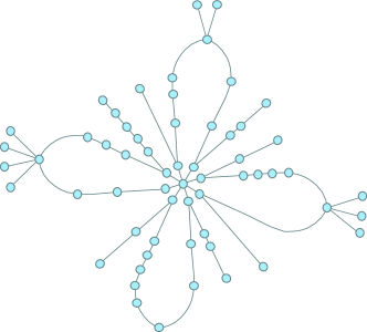
Figure 1: An example of a snowflake graph

Definition 2.4 ([15]).

The pathwidth of a graph $G$ is defined using its path decomposition, which is a sequence of subsets of vertices $\{X_{1},X_{2},\dots,X_{k}\}$, called bags, such that every vertex $v\in V$ appears in at least one bag and, for every edge $(u,v)\in E$, there exists a bag $X_{i}$ containing both $u$ and $v$. Furthermore, if a vertex $v\in V$ appears in two bags $X_{i}$ and $X_{j}$, it must also appear in all bags $X_{h}$ for $i\leq h\leq j$, ensuring a contiguous layout of $v$ in the sequence. The pathwidth of $G$ is the size of the largest bag in such a decomposition, minus one.

Observation 2.1.

Snowflake graphs have a pathwidth of at most 2.

Proof. Removing the center from a snowflake graph results in a collection of disjoint caterpillar graphs, each with a pathwidth of 1. Consider the path decomposition of the caterpillars. Reintroducing the center by adding it to every bag in the path decomposition constructs a valid path decomposition. Adding the center increases the pathwidth by at most 1, resulting in a pathwidth of 2 for snowflake graphs. $\Box$

3 Cactus Broadcaster: A 2-Approximation Algorithm for Cactus Graphs

This section begins by introducing a novel model, referred to as the multi-broadcasting model. Building on this foundation, we propose an algorithm that achieves a 2-approximation polynomial algorithm.

3.1 Multi-broadcasting Model

In the multi-broadcasting model, with parameter $k$, an informed vertex can simultaneously inform up to $k$ neighbors in a single round, a process we refer to as a super call. This model is closely related to the $k$-broadcasting problem, a variant of Telephone Broadcasting where an informed vertex can notify up to $k$ neighbors in each round. Grigni and Peleg [8] derived a tight bound for the $k$-broadcasting time $\mathcal{B}\boldsymbol{r}_{k}$ for a graph of size $n$, demonstrating that $\mathcal{B}\boldsymbol{r}_{k}\in\Theta(kL_{k}(n)n)$. In this expression, $L_{k}(n)$ represents the exact number of consecutive leading $k$s in the $(k+1)$-ary representation of $n-1$. Later, Harutyunyan and Liestman [10] improved this result for almost all values of $k$ and $n$. In contrast, the classic model allows each vertex to inform at most one of its uninformed neighbors per round. We will present a method to convert a broadcasting schema in the multi-broadcasting model into the classic model (without super calls). The final number of rounds in the classic model will be at most $k$ times the number of rounds in the multi-broadcasting model. Note that this model, along with the following lemma, applies not only to cactus graphs but also to every arbitrary graph. For the case of cactus graphs, we just need the case of $k=2$.

Lemma 3.1.

There is a polynomial algorithm that converts a broadcasting schema in the multi-broadcasting model to the classic model by keeping the broadcasting scheme valid and the total number of rounds at most $k$ times the number of rounds in the multi-broadcasting model.

Proof. To convert the multi-broadcasting model into the classic model, note that in the multi-broadcasting model, some informed nodes simultaneously inform up to $k$ uninformed neighbors. Let the total number of rounds in the multi-broadcasting model be $\mathcal{B}\boldsymbol{r}$. During the conversion, for each round $r\in[\mathcal{B}\boldsymbol{r}]$, the $k$ neighbors are informed sequentially in the classic model across $k$ separate rounds. Specifically, the first neighbor is informed in round $k(r-1)+1$, the second in $k(r-1)+2$, and so on, up to the $k$-th neighbor in $kr$. This ensures that the total number of classic rounds after conversion is at most $k\mathcal{B}\boldsymbol{r}$. The broadcasting scheme remains valid, as every informed node informs at most one neighbor in each classic round. Figure 2 shows an example of this conversion. $\Box$

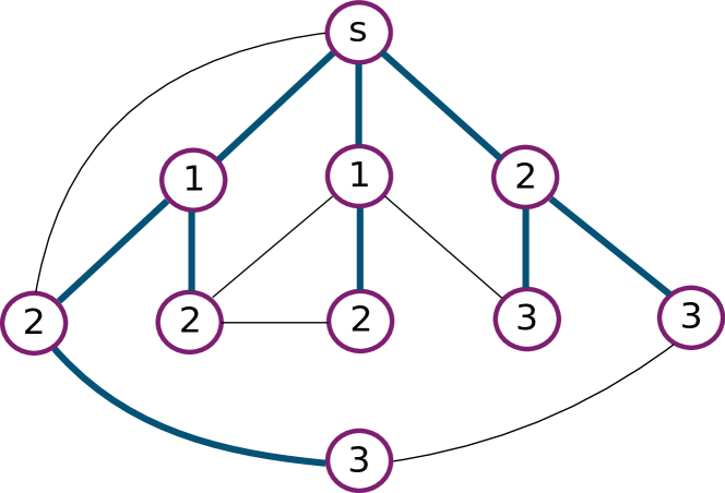
(a) The rounds in which each node is broadcasted in the multi-broadcasting model with $k=2$ are shown, where each informed node can simultaneously inform at most two uninformed neighbors per super round.

(b) The rounds in which each node is broadcasted in the classic model are shown, with each super round $r\in[\mathcal{B}\boldsymbol{r}]$ splits into two classic rounds of $2r-1$ and $2r$.

Figure 2: An example demonstrating the conversion process from the multi-broadcasting model to the classic model for the case of $k=2$. Highlighted edges represent the message propagation paths within the graph, and the numbers indicate the rounds in which nodes get informed.

3.2 Cactus Broadcaster Algorithm

This subsection presents Cactus Broadcaster, a 2-approximation algorithm for the Telephone Broadcasting problem on cactus graphs. It is a mutually recursive algorithm with two main functions: single-source-broadcaster($G,s$) and double-source-broadcaster($G,s_{1},s_{2}$). The single-source-broadcaster($G,s$) function is used to broadcast a connected subgraph $G$ using only one source $s$. The double-source-broadcaster($G,s_{1},s_{2}$) function is used to broadcast a connected subgraph $G$ using two sources $s_{1}$ and $s_{2}$ given that $s_{1}$ and $s_{2}$ are connected by a path in which every edge is a cut-edge, or in other words they used to be in a cycle together in the original graph. Note that a cut-edge is an edge in a graph whose removal increases the number of connected components.

  Input: A graph $G$ and a source node $s$.

  Output: The total broadcasting time of the algorithm on $G$ with source node $s$.

1: $\textit{broadcast\_times}\leftarrow\{\}$

2: for each connected component $G_{i}\in G\setminus\{s\}$ do

3:  if the component contains a single neighbor $v_{i}$ of $s$ then

4:   time $\leftarrow$ single-source-broadcaster($G_{i},v_{i}$)

5:  else if the component contains two neighbors $v_{i}$ and $u_{i}$ of $s$ then

6:   time $\leftarrow$ double-source-broadcaster($G_{i},v_{i},u_{i}$)

7:  broadcast_times $\leftarrow$ broadcast_times $\cup$ {time}

8: Sort broadcast_times in descending order

9: $\textit{max\_time}\leftarrow 0$

10: $\textit{num\_components}\leftarrow\text{length}(\textit{broadcast\_times})$

11: for $i$ in num_components do

12:  $\textit{total\_time}\leftarrow(i+1)+\textit{broadcast\_times}[i]$

13:  $\textit{max\_time}\leftarrow\max(\textit{max\_time},\textit{total\_time})$

14: return max_time

Algorithm 1 single-source-broadcaster($G,s$)

The single-source-broadcaster($G,s$) operates as follows: Removing the source node $s$ partitions its subgraph into disjoint connected components, each containing one or two of its immediate neighbors. Refer to Figure 3 for an example of the possible cases of connected components after removing the source. Importantly, a single subgraph cannot have more than two neighbors of the source, as all neighbors in the subgraph must be connected. Having more than two neighbors would imply an edge belonging to two cycles, which is impossible in cactus graphs. For each component $i$ with a single neighbor $v_{i}$, the broadcasting time is computed as single-source-broadcaster($G,v_{i}$) plus one round to inform $v_{i}$ using a classic call. For components $i$ with two neighbors $v_{i}$ and $u_{i}$, the broadcasting time is computed as double-source-broadcaster($G,v_{i},u_{i}$) plus one round to inform both $v_{i}$ and $u_{i}$ simultaneously using a super call.

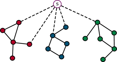
Figure 3: Two possible types for broadcasting to connected components after deleting $s$ in single-source-broadcaster($G,s$) are shown. In the first type, a super call is used to simultaneously inform the two red neighbours of $s$ (or its two blue neighbours). In the second type, the sole green neighbour of $s$ is informed via a regular call.

After calculating the broadcasting times for all components, we sort these values in descending order. We inform the component with the largest broadcasting time in the first round, the second-largest in the second round, and so on. This prioritization ensures that the subgraphs with the largest broadcasting times have the maximum remaining time for their sources to inform their subgraphs before the end of broadcasting. The final answer is the maximum value obtained by summing the round in which a component was informed and the total rounds needed to inform its entire subgraph. A pseudocode of this algorithm is provided in Algorithm 1.

  Input: A graph $G$ and two source nodes $s_{1}$ and $s_{2}$.

  Output: The total broadcasting time of the algorithm for $G$ given that $s_{1}$ and $s_{2}$ are informed.

1: $\textit{min\_broadcast\_time}\leftarrow\infty$

2: for each edge $e$ in the cycle of $G$ do

3:  $G_{e}\leftarrow G\setminus\{e\}$

4:  $G_{1}\leftarrow G_{e}\cap\text{vertices reachable from }s_{1}$

5:  $G_{2}\leftarrow G_{e}\cap\text{vertices reachable from }s_{2}$

6:  $T_{1}\leftarrow$single-source-broadcaster($G_{1},s_{1}$).

7:  $T_{2}\leftarrow$single-source-broadcaster($G_{2},s_{2}$).

8:  $\textit{broadcast\_time}\leftarrow\max(T_{1},T_{2})$.

9:  $\textit{min\_broadcast\_time}\leftarrow\min(\textit{min\_broadcast\_time},\textit{broadcast\_time})$.

10: return min_broadcast_time

Algorithm 2 double-source-broadcaster($G,s_{1},s_{2}$)

We outline the functionality of the double-source-broadcaster($G,s_{1},s_{2}$). Consider any valid broadcasting scheme, let informing edges be edges along which the message is propagated in the scheme. The informing edges form a spanning tree as it does not admit any cycle and covers all nodes.

As double-source-broadcaster also finds a broadcasting scheme, one edge from each cycle must be excluded. Thus, we need to remove one edge of the cycle containing $s_{1}$ and $s_{2}$ and broadcast the two disjoint parts of the graph through their respective inform nodes, $s_{1}$ or $s_{2}$. This exclusion is essential because attempting to broadcast using all edges of a cycle would result in a node being informed by two different neighbors, which is not feasible. Refer to Figure 4 for an example of the exclusion and the resulting subgraphs for $s_{1}$ and $s_{2}$.

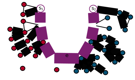
Figure 4: The connected subgraphs containing $s_{1}$ and $s_{2}$ after the exclusion of edge $e$ are shown in double-source-broadcaster. single-source-broadcaster can then be applied to each of the subgraphs with $s_{1}$ and $s_{2}$ as sources.

The algorithm evaluates all possible edges in the cycle, removes each one individually, and selects the edge that minimizes the total number of broadcasting rounds. Since excluding an edge from the cycle ensures that the immediate edge of the source $s_{1}$ or $s_{2}$ is no longer part of a cycle connected to the other source, we can independently apply single-source-broadcaster to $s_{1}$ and $s_{2}$ to handle their respective subgraphs. The overall broadcast time for the graph is then determined as the maximum of these two values. A pseudocode of this algorithm is provided in Algorithm 2.

For the last step, Cactus Broadcaster uses the method in Lemma 3.1 to transform the broadcasting scheme from the two functions mentioned above in the multi-broadcasting model, which includes super rounds, into a solution for the slow model consisting only of classic rounds.

Theorem 3.2.

Cactus Broadcaster is a polynomial-time algorithm for Telephone Broadcasting that achieves an approximation ratio of $2$ on cactus graphs.

To establish the theorem, we need to prove the following lemmas.

Lemma 3.3.

Cactus Broadcaster terminates in polynomial time.

Proof. In the double-source-broadcaster($G,s_{1},s_{2}$), the naive approach of checking all possible edge exclusions is exponential, as each node in the cycle can have attached subgraphs. This results in repeatedly calling the functions on subgraphs for each node. To optimize, we first calculate the broadcast time for the connected subgraphs after deleting the main cycle (the cycle in the original graph includes $s_{1}$ to $s_{2}$). An example of this approach is illustrated in Figure 5. Next, we select an edge in the main cycle to exclude and start the process from the node immediately adjacent to the excluded edge.

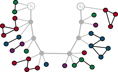
Figure 5: The resulting connected components, formed after deleting the nodes of the main cycle, are shown in different colors. The algorithm precomputes the broadcasting times for each connected component before edge exclusion in double-source-broadcaster.

Consider the part of the graph that needs to be informed by $s_{1}$. Starting with the node immediately adjacent to the excluded edge, we compute the broadcast time for its subgraph using precomputed values and do the same thing as we do in single-source-broadcaster, sorting based on the broadcasting time we found in descending order and informing them one by one. At last, store the result as $t_{\text{acc}}$. Moving to its neighbor in the main cycle, which is closer to $s_{1}$ and treated as its immediate parent, we incorporate $t_{\text{acc}}$ as the broadcasting time for another subgraph of it. We then sort the precomputed values for the subgraphs outside the main cycle along with $t_{\text{acc}}$. This process is repeated iteratively, moving toward $s_{1}$, until the total broadcast time is determined using single-source-broadcaster($G^{e}_{1},s_{1}$), where $G^{e}_{1}$ represents the part of $G$ connected to $s_{1}$ after removing the edge $e$ from the path. Figure 6 shows an example of this approach.

Figure 6: The resulting connected components for the purple node are shown after incorporating the subgraphs. The algorithm sorts the blue, red, and incorporated green components based on their broadcast times and then computes the broadcast time for the entire subgraph of the purple node.

The same procedure is applied for $s_{2}$, and by taking the maximum of the results from both $s_{1}$ and $s_{2}$, the algorithm determines the total broadcast time for the entire graph after removing the edge $e$. Thus, the maximum time required is $O(n.n.\log(n))$ for a graph with $n$ nodes.

To prove that the time complexity is $O(n^{3}\log(n))$, we define the following functions. The function $T_{1}(n)$ and $T_{2}(n)$ represent the maximum time required to process a subgraph of size $n$ using single-source-broadcaster and double-source-broadcaster, respectively. Let $T(n)$ be the maximum of these two functions.

single-source-broadcaster involves running the sub-functions with time $T(n_{i})$ on all the immediate neighbors of the source, along with an additional $O(n.\log(n))$ time to sort the subgraphs by the broadcasting times obtained from sub-functions. On the other hand, double-source-broadcaster includes precomputing the broadcast time for the subgraphs after deleting the nodes of the main cycle and, for each excluded edge, sorting the subgraphs while propagating toward the source, which takes $O(n.n.\log(n))$ time. For each $n$, set $H_{n}$ can be any set of positive integers $n_{i}$ such that $\sum n_{i}<n$.

$$T(n) =\max(T_{1}(n),T_{2}(n))$$

$$T_{1}(n) \leq\max_{H_{n}}\sum_{n_{i}\in H_{n}}T(n_{i})+O(n.\log(n))$$

$$T_{2}(n) \leq\max_{H_{n}}\sum_{n_{i}\in H_{n}}T(n_{i})+O(n.n.\log(n))$$

We use induction to prove that $T(n)\leq cn^{3}.\log(n)$, assuming $T(j)\leq cj^{3}.\log(j)$ for all $j<n$, in which $c$ is a constant number. Since $T_{1}(n)$ has a lower complexity than $T_{2}(n)$ and $T(n)$ is determined as the maximum of the two, it suffices to prove the result for $T_{2}(n)$:

$$T_{2}(n) \leq\max_{H_{n}}\sum_{n_{i}\in{H_{n}}}T(n_{i})+c^{\prime}n^{2}.\log(n)$$

$$\leq\max_{H_{n}}\sum_{n_{i}\in{H_{n}}}c.n_{i}^{3}.\log(i)+c^{\prime}n^{2}.\log(n)$$ using induction hypothesis

$$\leq c(n-1)^{3}.\log(n)+c^{\prime}n^{2}.\log(n) \max_{H_{n}}\sum_{n_{i}\in H_{n}}n_{i}<n$$

$$\leq(cn^{3}-cn^{2}).\log(n)+c^{\prime}n^{2}.\log(n)$$

$$\leq cn^{3}.\log(n) c\geq c^{\prime}$$ assuming

The lemma is proven through induction, with the base case being a graph containing a single source node that is already informed and letting the maximum time be at most $c$ in the base cases by setting $c$ large enough. $\Box$

Lemma 3.4.

The number of super rounds in Cactus Broadcaster does not exceed the number of rounds used by the optimal solution in the classic model.

Proof. We use induction on the number of nodes in the graph to prove the claim for both recursive functions single-source-broadcaster and double-source-broadcaster. In the base case, the graph consists of just informed nodes making the statement trivially true. For the inductive step, we aim to prove the claim for a graph with $n>1$ nodes, assuming it holds for all graphs with $j<n$ nodes.

First, we consider the double-source-broadcaster($G,s_{1},s_{2}$). The algorithm evaluates the removal of each edge in the cycle containing $s_{1}$ and $s_{2}$, selecting the edge $e$ that minimizes the total broadcasting time. Let the removal of edge $e$ partition the graph into two subgraphs, $G^{e}_{1}$ and $G^{e}_{2}$, to be broadcasted by $s_{1}$ and $s_{2}$, respectively. The broadcasting time for the graph is then determined based on these two subgraphs as follows,

$$\texttt{double-source-broadcaster($G,s_{1},s_{2}$)}=\min_{e}\max( \texttt{single-source-broadcaster($G^{e}_{1},s_{1}$)},$$

$$\texttt{single-source-broadcaster($G^{e}_{2},s_{2}$)})$$

Assume that the optimal solution removes an edge $e^{*}$ from the main cycle. Base on the induction hypothesis we know that $\texttt{single-source-broadcaster($G^{e^{*}}_{1},s_{1}$)}\leq OPT(G^{e^{*}}_{1},s_{1})$ and $\texttt{single-source-broadcaster($G^{e^{*}}_{2},s_{2}$)}\leq OPT(G^{e^{*}}_{2},s_{2})$. In this case, the broadcast time of the optimal solution would be

$$\mathcal{B}\boldsymbol{r}(OPT)=\max(OPT(G^{e^{*}}_{1},s_{1}),OPT(G^{e^{*}}_{2},s_{2}))$$

Since the algorithm identifies the edge removal that minimizes the broadcast time, we have $\mathcal{B}\boldsymbol{r}(ALG)\leq\mathcal{B}\boldsymbol{r}(OPT)$, ensuring that the algorithm’s broadcast time is at most that of the optimal solution.

Next, we address the case of the single-source-broadcaster. Upon removing the source, the graph splits into several connected disjoint components. These components are then sorted by the broadcasting times obtained from sub-functions, which are either single-source-broadcaster or double-source-broadcaster depending on the condition. In the algorithm, the neighbor(s) belonging to the largest broadcasting time is informed first, as this provides the maximum time to broadcast the message within its subgraph. The neighbor(s) in the second-largest broadcasting time is informed next, and so on.

The total broadcast time is determined by the maximum of the times it takes for each component to be fully broadcast after receiving information from the source, plus the time it takes for the source or sources to be informed.

Consider the optimal broadcasting scheme in the classic model. For a component $C_{i}$ with two sources, the time at which the first source is informed optimally is denoted by $\pi^{1}_{i}$, and the time at which the second source (if exists) is informed optimally is denoted by $\pi^{2}_{i}$, where $\pi^{1}_{i}<\pi^{2}_{i}$. If both sources were informed simultaneously via a super call at $\pi^{1}_{i}$, the broadcast time would get reduced compared to informing the first source at $\pi^{1}_{i}$ and waiting until $\pi^{2}_{i}$ to inform the second one. Thus, the following inequality holds:

$$\mathcal{B}\boldsymbol{r}(OPT)=\max_{i}(OPT(C_{i},(\pi^{1}_{i},\pi^{2}_{i}))) \geq\max_{i}(OPT(C_{i},(\pi^{1}_{i},\pi^{1}_{i})))$$

$$=\max_{i}(OPT(C_{i},(0,0)))+\pi^{1}_{i}$$

where $OPT(C_{i},(\pi^{1}_{i},\pi^{2}_{i}))$ is the optimal broadcasting time in the classic model given that the first source is informed at round $\pi^{1}_{i}$ and the second one (if exists) at round $\pi^{2}_{i}$. Denote the recursively found broadcast time for each component $C_{i}$ as $r_{i}$, which is determined by applying the subfunctions on $C_{i}$. This is equivalent to informing the entire component $C_{i}$ at time $0$.

$$\mathcal{B}\boldsymbol{r}(OPT) \geq\max_{i}(OPT(C_{i},(0,0)))+\pi^{1}_{i}$$

$$\geq\max_{i}(r_{i}+\pi^{1}_{i}) OPT(C_{i},(0,0))\geq r_{i}$$

$$\geq\min_{\pi^{\prime}}(\max_{i}(r_{i}+\pi^{\prime}_{i}))=\mathcal{B}\boldsymbol{r}(ALG)$$

The algorithm chooses $\pi^{\prime}_{i}$ such that $\max_{i}(r_{i}+\pi^{\prime}_{i})$ is minimized. This is ensured by sorting the times required to inform each subgraph in descending order and informing the neighbor(s) responsible for the subgraphs accordingly. Thus, $\mathcal{B}\boldsymbol{r}(\text{OPT})\geq\mathcal{B}\boldsymbol{r}(\text{ALG})$. As the lemma holds for both functions, it is proved. $\Box$

Proof of Theorem 3.2: By Lemma 3.3, we demonstrated that Cactus Broadcaster terminates in polynomial time. Furthermore, Lemmas 3.4 and 3.1 establish that Cactus Broadcaster’s broadcasting time is at most twice that of the optimal. This concludes the proof. $\Box$

4 Hardness Proof of Snowflake Graphs

The NP-hardness proof of Telephone Broadcasting in snowflake graphs proceeds through successive reductions: $3,4$-SAT to Twin Interval Selection, Dome Selection with Prefix Restrictions, Compatible Dome Selection, and finally Telephone Broadguess. To provide clarity, we first define the problems that form the foundation of our hardness proof.

Definition 4.1.

The $3,4$-SAT problem is a variant of the classical $3$-satisfiability ($3$-SAT) problem that imposes additional structural constraints on the input formula. It takes as input a boolean formula $\phi$ in the conjunctive normal form (CNF) with two key properties: each clause contains exactly three literals, and each variable appears in at most four clauses of $\phi$. The problem is whether there is a way of assigning boolean values to the variables that satisfy all constraints.

The $3,4$-SAT problem is known to be NP-complete [19].

Definition 4.2.

The Twin Interval Selection problem involves a pair input $(I,r)$, where $I=\{(I_{1},\overline{I_{1}}),(I_{2},\overline{I_{2}}),\dots,(I_{n},\overline{I_{n}})\}$ is a set of pairs of non-overlapping intervals of equal length called twin intervals. For each pair $(I_{i},\overline{I_{i}})$ we should select one of them. A restriction function $r:[m]\to[n]$ specifies the maximum allowed number of selected intervals at each time $t\in[m]$, in which the value $m$ denotes the largest endpoint of any interval in $I$. In other words, for any given time $t$, the number of selected intervals that include $t$ should be less than or equal to $r(t)$. The goal is to determine whether there is a valid selection that satisfies these restrictions.

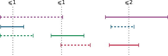
Figure 7: An instance of Twin Interval Selection is shown, where each pair of twin intervals is represented with the same color and height. Dotted intervals indicate unselected intervals, while solid intervals represent selected ones. The restriction is shown at three points, indicating that the total number of selected intervals at these times must not exceed the specified limits. One can readily check that the selected intervals form a valid solution.

An instance of Twin Interval Selection is shown in Figure 7. Before defining the next two problems, we first define a dome.

Definition 4.3.

A dome $(a,b,c,d)$ is defined as a set of at most two arcs $(a,d)$ and $(b,c)$ such that $a\leq b<c\leq d$ and $b-a=d-c$. When $(a,d)=(b,c)$, i.e., the dome consists of exactly one arc, we call it a singleton dome, and a regular dome otherwise, as illustrated in Figures 10 and 11 respectively.

The following two problems are defined over a set of domes $D=\{D_{1},D_{2},\dots,D_{n}\}$, where each dome $D_{i}$ is defined by two arcs with endpoints $(a_{i},d_{i})$ and $(b_{i},c_{i})$, such that $a_{i}\leq b_{i}<c_{i}\leq d_{i}$, and $b-a=d-c$. The maximum existing endpoint in $D$ is represented as $m$.

Definition 4.4.

The Dome Selection with Prefix Restrictions problem requires selecting exactly one arc for each dome, ensuring that at any time $t$, the total number of endpoints from the selected arcs lying at or before $t$ does not exceed $t$. The objective is to determine whether such a valid selection of arcs exists that satisfies these constraints.

Definition 4.5.

The Compatible Dome Selection problem aims to determine whether a valid selection of arcs, possibly shifted to the left, can be disjoint on their endpoints. In other words, for each dome, exactly one arc should be selected, which may either remain unchanged or be shifted to the left (each endpoint individually). The only condition is that the final selected endpoints must be distinct.

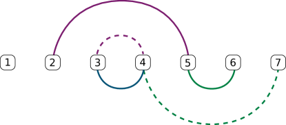
Figure 8: An instance of Dome Selection with Prefix Restrictions is shown, where each pair of arcs in a dome is represented with the same color. Dotted arcs denote unselected arcs, while solid arcs indicate selected ones. For the singleton dome, its only arc is always selected. The restriction of Dome Selection with Prefix Restrictions is satisfied in the presented solution, as for each time $t$, the number of selected endpoints preceding it is less than or equal to $t$. This instance can also be interpreted as an instance of Compatible Dome Selection, where the selected arcs can be shifted left, provided that the endpoints at each time remain distinct. This is achieved by keeping the purple and blue selected arcs at their locations while shifting the left endpoint of the selected green arc to time $t=1$.

An instance of Dome Selection with Prefix Restrictions and Compatible Dome Selection is shown in Figure 8.

Definition 4.6.

The Telephone Broadguess problem is the decision variant of the Telephone Broadcasting Problem. The input $(G,s,\mathcal{B}\boldsymbol{r})$, consists of a graph $G$, a vertex $s$ designated as the source node for information dissemination, and an integer value $\mathcal{B}\boldsymbol{r}$. The process begins having vertex $s$ informed in the first round. In each subsequent round, every informed vertex can inform at most one of its uninformed neighbors. The problem is whether it is possible to spread the information from $s$ to all vertices in $G$ within $\mathcal{B}\boldsymbol{r}$ rounds.

4.1 Reduction from 3,4-SAT to Twin Interval Selection

The first step in reducing $3,4$-SAT to Telephone Broadguess is to establish a reduction from $3,4$-SAT to Twin Interval Selection. This can be achieved by constructing a Twin Interval Selection instance for any given $3,4$-SAT instance and demonstrating the equivalence of solutions between the two problems.

4.1.1 Construction

Given an instance $\phi=(X,C)$ of $3,4$-SAT, we construct an instance of Twin Interval Selection as follows. For each variable $x_{i}\in X$ in the $3,4$-SAT instance, construct a pair of twin intervals, each of length $7$. The interval $[16i-16,16i-9]$ represents $x_{i}$, while $[16i-8,16i-1]$ represents $\overline{x_{i}}$.

Regarding clause gadgets, for each clause $C^{j}\in C$ and every literal $C^{j}_{k}\in C^{j}$, create a twin interval pair of unit length. The first interval is positioned at $[s+2q,s+2q+1]$, considering $s$ is the first endpoint of the interval associated with $\overline{C_{k}^{j}}$ and $C^{j}$ is the $q$-th occurrence of literal $C^{j}_{k}$. Moreover, the position of the second interval is $[16n+2j,16n+2j+1]$, in which $n=|X|$. Finally, regarding the restriction function, $r(t)=1$ for all $t\leq 16n$ and $r(t)=2$, otherwise.

Moreover, as the number of twin intervals is $|X|+|C|$, and the maximum time that we use is $16|X|+2|C|+1$, the reduction is polynomial.

4.1.2 Proof of Equivalence

To complete the reduction, we must establish the equivalence between instances of $3,4$-SAT and the constructed Twin Interval Selection instance.

Lemma 4.7.

Given a $3,4$-SAT instance $\phi$ and its corresponding Twin Interval Selection instance $\mathcal{I}_{\phi}$, $\phi$ is satisfiable if and only if $\mathcal{I}_{\phi}$ admits a valid selection of intervals.

We prove Lemma 4.7 with Lemma 4.8 and Lemma 4.9.

Lemma 4.8.

If $\phi$ is satisfiable, then $\mathcal{I}_{\phi}$ admits a valid interval selection.

Proof. Let $\sigma:X\to\{0,1\}$ be a satisfying assignment for $\phi$, where $X$ is the set of variables in $\phi$. We construct a selection $S$ for $\mathcal{I}_{\phi}$. For each variable $x_{i}\in X$, if $\sigma(x_{i})=1$, we select the interval associated with $x_{i}$ in $\mathcal{I}_{\phi}$ alongside the right intervals of all the clause gadget twin intervals that are related to literal $\overline{x_{i}}$ and the left intervals of all the ones related to literal $x_{i}$, and if $\sigma(x_{i})=1$, we select the exactly the opposite intervals of the previous case for each twin.

We now prove that $S$ satisfies all restrictions in $\mathcal{I}_{\phi}$. For $t>16n$, based on our construction, either zero or three intervals pass through these points. In the case of three intervals, one for each literal in the corresponding clause intersects with each other. Since $\sigma$ satisfies $\phi$, at least one literal in each clause is true. As a result, at least one of them is not selected. This ensures that the sum of values at these points is at most two, satisfying the restriction.

For $t\leq 16n$, at most two intervals pass through any such point of time. Also, based on the definition of $S$, whenever we choose an interval related to a variable, we do not choose the left intervals of the clause gadgets that intersect with it. Note that the right intervals of all clause gadgets are disjoint from the twin intervals related to the variables. Consequently, the sum of values at these points is at most $1$, satisfying the restriction $r(t)=1$. Thus, $S$ is a valid selection for $\mathcal{I}_{\phi}$.

$\Box$

Lemma 4.9.

If $\mathcal{I}_{\phi}$ admits a valid interval selection, then $\phi$ is satisfiable.

Proof. Let $S$ be a valid selection of intervals for $\mathcal{I}_{\phi}$. We construct an assignment $\sigma:X\to\{0,1\}$ for $\phi$ as follows: For each variable $x_{i}\in X$, set $\sigma(x_{i})=1$ if the interval associated with $x_{i}$ is in $S$, and set $\sigma(x_{i})=0$, otherwise.

We want to prove that $\sigma$ satisfies $\phi$. By construction, for each clause $C_{j}$ we know that all three right intervals of the twin intervals corresponding to three literals of $C_{j}$ contain time $16n+2j$. As $16n+2j>16n$, $r(t)=2$. Thus, at least one of these three intervals should not be selected in $S$. Thus, consider $C^{j}_{k}$ is the one that the left interval of its corresponding twin interval in the clause gadget is selected. Because the left interval overlaps with the variable gadget corresponding to $\overline{C^{j}_{k}}$ at some time $t$, and $r(t)=1$, the twin interval in the variable gadget related to $\overline{C^{j}_{k}}$ cannot be selected in $S$, thus $S$ must select the other interval in that twin, which is $C^{j}_{k}$. Therefore, $\sigma(C^{j}_{k})=1$. Consequently, each clause $C_{j}$ in $\phi$ has at least one true literal under $\sigma$. Therefore, $\sigma$ satisfies $\phi$.

$\Box$

Proof of Lemma 4.7: Based on Lemma 4.8 and 4.9, we have established that the $3,4$-SAT instance $\phi$ is satisfiable if and only if the constructed Twin Interval Selection instance $\mathcal{I}_{\phi}$ admits a valid selection. This completes the proof of equivalence and validates the reduction from $3,4$-SAT to Twin Interval Selection. $\Box$

4.2 Reduction from Twin Interval Selection to Dome Selection with Prefix Restrictions

Building upon our previously established reduction from $3,4$-SAT to Twin Interval Selection, we present a polynomial-time reduction from Twin Interval Selection to Dome Selection with Prefix Restrictions. Our approach involves constructing a Dome Selection with Prefix Restrictions instance from any given Twin Interval Selection instance and formally proving the equivalence of solutions between the two problems.

4.2.1 Construction

Given an arbitrary instance $\mathcal{I}$ of Twin Interval Selection, we construct the corresponding instance of Dome Selection with Prefix Restrictions as follows. For each pair of intervals $(I_{i},\bar{I_{i}})\in\mathcal{I}$, let $I_{i}=(a,b)$ and $\bar{I_{i}}=(c,d)$. We construct a regular dome for each interval pair by creating two arcs: one spans from $2a$ to $2d+1$, and the other spans from $2b+1$ to $2c$. Next, we apply a scaling factor of $3n$ to all endpoints in the timeline, where $n$ is the number of interval pairs in $\mathcal{I}$. The domes are scaled accordingly.

After scaling the timeline, additional domes, called singleton domes, are introduced. These singleton domes consist of a single arc with one endpoint at some point $t$ and the other at a point $t^{\prime}$, where $t^{\prime}$ is chosen to be after all other dome endpoints. Each singleton dome is assigned to a unique $t^{\prime}$. After adding all the singleton domes, the maximum time in Dome Selection with Prefix Restrictions is denoted as $m$, which is used in the rest of this section.

The number of singleton domes added at any point $t$ is determined by the function $d(t)$. If $t$ is a multiple of $6n$, then:

$$d(t)=t-c_{t}-\sum_{j<t}d(j)-r(t/6n),$$

and $d(t)=0$ otherwise. Here, $c_{t}=2|\mathfrak{D}_{4}^{t}|+|\mathfrak{D}_{3}^{t}|+|\mathfrak{D}_{2}^{t}|$, where $\mathfrak{D}_{i}^{t}$ represents the set of regular domes with exactly $i$ endpoints before or at time $t$. Figure 9 illustrates these dome types. Additionally, $r(t/6n)$ represents the restriction value at the point corresponding to $t$ in the original instance $\mathcal{I}$ (the corresponding time before scaling). It will be shown, in Observation 4.1, that $d(t)$ is always non-negative.

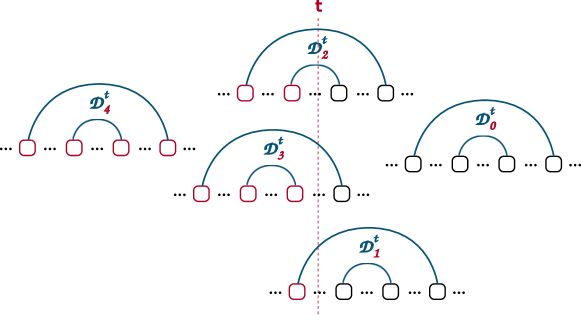
Figure 9: Different types of domes are shown, classified based on their positions relative to time $t$, where $\mathfrak{D}_{i}^{t}$ denotes the set of regular domes with $i$ endpoints at or before $t$.

4.2.2 Proof of Equivalence

To prove the reduction, we first need to establish the equivalence of solutions between the two problems. Additionally, we must demonstrate that they can be converted into each other in polynomial time based on the input size.

One can readily verify that the reduction operates in polynomial time. The timeline is expanded by a factor of $6n$, and a new time point is added for each singleton dome. Furthermore, the total number of singleton domes is bounded by $\mu^{2}$, where $\mu$ represents the maximum time of $\mathcal{I}$.

Observation 4.1.

$d(t)$ in the above construction cannot be negative.

Proof. Since for any $t$ that is not divisible by $6n$, $d(t)=0$ by definition, the lemma holds. When $t$ is divisible by $6n$, we have:

$$d(t) =t-c_{t}-\Sigma_{j<t}d(j)-r(t/6n)$$

$$=t-c_{t}-\Sigma_{j\leq(t-6n)}d(j)-r(t/6n)$$

$\Sigma_{j<t}d(j)=\Sigma_{j\leq(t-6n)}d(j)$ because any values of $d(j)$ between $t-6n$, the previous discreet multiple of $6n$, and $t$, the current discreet multiple of $6n$, is $0$.

$$d(t) =t-c_{t}-d(t-6n)-\Sigma_{j<t-6n}d(j)-r(t/6n)$$

$$=t-c_{t}-((t-6n)-c_{t-6n}-\Sigma_{j<t-6n}d(j)-r(\frac{t-6n}{6n}))-\Sigma_{j<t-6n}d(j)-r(t/6n)$$

$$=-c_{t}+6n+c_{t-6n}+r(\frac{t-6n}{6n})-r(t/6n)$$

As $c_{t-6n}$ and $r(\frac{t-6n}{6n})$ are both non-negative, and by definition, $r(t/6n)$ is at most $n$, we can conclude that:

$$d(t)\geq-c_{t}+6n-r(t/6n)\geq 5n-c_{t}$$

Next, we bound $c_{t}$ as follows:

$$c_{t}=2|\mathfrak{D}_{4}^{t}|+|\mathfrak{D}_{3}^{t}|+|\mathfrak{D}_{2}^{t}|\leq 2(|\mathfrak{D}_{4}^{t}|+|\mathfrak{D}_{3}^{t}|+|\mathfrak{D}_{2}^{t}|)\leq 2n$$

Thus, $d(t)\geq 5n-c_{t}\geq 3n$, which is non-negative. $\Box$

Observation 4.2.

For each dome $(a,b,c,d)$, we have $b-a=d-c$.

Proof. For each twin of intervals $I_{1}=(a^{\prime},b^{\prime})$ and $I_{2}=(c^{\prime},d^{\prime})$, and the length of intervals are the same, meaning $b^{\prime}-a^{\prime}=d^{\prime}-c^{\prime}$. Multiplying by two and adding one to each side, we have $(2b^{\prime}+1)-2a^{\prime}=(2d^{\prime}+1)-2c^{\prime}$. Based on the way of construction, the corresponding domes will be from $2a^{\prime}$ to $2d^{\prime}+1$, named as $a$ and $d$, and $2b^{\prime}+1$ to $2c^{\prime}$, named as $b$ and $c$. Thus, $b-a$ is equal to $(2b^{\prime}+1)-2a^{\prime}$ and $d-c$ is equal to $(2d^{\prime}+1)-2c^{\prime}$. The final scaling factor of $3n$ can be added to both sides of the equation without altering its validity. $\Box$

Lemma 4.10.

Consider $\mathcal{I}$ as an instance of Twin Interval Selection and $\mathcal{D}$ as the corresponding instance of Dome Selection with Prefix Restrictions. If $\mathcal{I}$ has a solution in Twin Interval Selection, then $\mathcal{D}$ has a solution in Dome Selection with Prefix Restrictions and vice versa.

First, we prove Lemma 4.11, which helps us for proving both sides of Lemma 4.10. Consider a solution $S$. Assume that for each dome $i$, the boolean value $x_{i}$ indicates whether the outer dome is selected in $S$. Specifically, $x_{i}=1$ refers to selecting the outer dome, while $\bar{x_{i}}=1$ refers to selecting the inner dome.

Lemma 4.11.

Given a solution $S$ of a Dome Selection with Prefix Restrictions instance, the number of chosen endpoints before or at the time $t$ is equal to $2|\mathfrak{D}_{4}^{t}|+|\mathfrak{D}_{3}^{t}|+\sum_{i\in\mathfrak{D}_{3}^{t}}\bar{x_{i}}+|\mathfrak{D}_{2}^{t}|+\sum_{i\in\mathfrak{D}_{1}^{t}}x_{i}+\sum_{j\leq t}d(j)$.

Proof. We structure the proof by dividing it into five cases, based on the time $t$ and the relative positions of the endpoints within each dome pair.

• For each dome with all $4$ endpoints before or at $t$, for each of the arcs, its two endpoints are before or at $t$, thus we have $2|\mathfrak{D}_{4}^{t}|$ endpoints.

• For each dome with exactly $3$ endpoints (all but the right endpoint of the outer arc) before or at $t$, by selecting any of the two arcs, the left endpoint of it is before or at $t$. However, selecting only the inner arc ensures that the right endpoint is at or before $t$, unlike the outer arc. Thus, we have $|\mathfrak{D}_{3}^{t}|+\sum_{i\in\mathfrak{D}_{3}^{t}}\bar{x_{i}}$ endpoints.

• For each dome with exactly $2$ endpoints (the left endpoint of each arc) before or at $t$, selecting either of them adds one endpoint to the number of chosen endpoints before $t$. Therefore, $|\mathfrak{D}_{2}^{t}|$ endpoints are before or at $t$.

• For each dome with exactly $1$ endpoint (right endpoint of the outer arc) before or at $t$, it only adds one to the number of endpoints when the outer arc is selected. Thus, the total number of these endpoints is $\sum_{i\in\mathfrak{D}_{1}^{t}}x_{i}$.

• Domes with all the endpoints after $t$ do not add any endpoints before or at it.

Considering the singleton domes added before time $t$, the proof of the lemma is complete. $\Box$

Lemma 4.12.

If $\mathcal{D}$ has a solution in Dome Selection with Prefix Restrictions, then $\mathcal{I}$ has a solution in Twin Interval Selection.

Proof. Consider a solution $S_{DSPR}$ of $\mathcal{D}$ in Dome Selection with Prefix Restrictions. We want to construct $S_{TIS}$ based on $S_{DSPR}$ and prove that it is a valid solution for $\mathcal{I}$. For each dome and its corresponding interval, if the inner arc is selected in $S_{DSPR}$, we select the right interval in $S_{TIS}$, and if the outer arc is selected by $S_{DSPR}$, we select the left interval in $S_{TIS}$.

We show that, in this way, for each time $t^{\prime}$ in $\mathcal{I}$, the number of selected intervals intersecting $t^{\prime}$ is less than or equal to $r(t^{\prime})$. In $S_{DSPR}$, the condition that is assumed to be satisfied is that the total number of endpoints of the selected arcs before or at time $t$ is less than or equal to $t$. Based on Lemma 4.11, we can derive the following inequality.

$$\sum_{i\in\mathfrak{D}_{3}^{t}}\bar{x_{i}}+\sum_{i\in\mathfrak{D}_{1}^{t}}x_{i} \leq t-c_{t}-\sum_{j\leq t}d(j)$$ (1)

$$=t-c_{t}-\sum_{j<t}d(j)-d(t)$$

$$=t-c_{t}-\sum_{j<t}d(j)-(t-c_{t}-\sum_{j<t}d(j)-r(t/6n))$$

$$=r(t/6n)$$ (2)

Thus, the right-hand side of the Inequality (2) is the restriction on the number of intersecting intervals in time $t^{\prime}=t/6n$. To complete the proof, we need to demonstrate that the left-hand side of Inequality (1) accurately represents the number of intersecting intervals at time $t^{\prime}$.

Consider a dome $i$, represented as $(a,b,c,d)$, with twin intervals $(a^{\prime},b^{\prime})$ and $(c^{\prime},d^{\prime})$. As $t=6t^{\prime}n$, $c=6nc^{\prime}$, and $d=6nd^{\prime}+3n$, one can imply that $t^{\prime}\in[c^{\prime},d^{\prime}]$ if and only if $i\in\mathfrak{D}_{3}^{t}$. The term $\sum_{i\in\mathfrak{D}_{3}^{t}}\bar{x_{i}}$ in Inequality (1) represents the domes in $\mathfrak{D}_{3}^{t}$ where the inner arc is selected, which corresponds to the intervals which their right intervals intersect time $t^{\prime}$ and are chosen. Similarly, the term $\sum_{i\in\mathfrak{D}_{1}^{t}}x_{i}$ calculates the number of left intervals selected which intersect time $t^{\prime}$. By summing these two cases, the left-hand side of the inequality represents the total number of selected intervals that intersect time $t^{\prime}$, while the right-hand side represents the constraint imposed for time $t^{\prime}$. Therefore $S_{TIS}$ is a valid solution for $\mathcal{I}$. $\Box$

Lemma 4.13.

If $\mathcal{I}$ has a solution in Twin Interval Selection, then $\mathcal{D}$ has a solution in Dome Selection with Prefix Restrictions.

Proof. Consider a solution $S_{TIS}$ of $\mathcal{I}$ in Twin Interval Selection. We want to construct $S_{DSPR}$ based on $S_{TIS}$ and prove that it is a valid solution for $\mathcal{D}$. For each dome and its corresponding interval, if the left interval is selected in $S_{TIS}$, we select the outer arc in $S_{DSPR}$, and if the right interval is selected $S_{TIS}$ we select the inner arc in $S_{DSPR}$.

In order to show that $S_{DSPR}$ is valid, we show that for each time $t$ in $\mathcal{D}$, the number of selected endpoints before or at $t$ is less than or equal to $t$. Note that based on the construction of $\mathcal{D}$, singleton nodes may be added with their right endpoints positioned after all existing endpoints. Let $m^{\prime}$ represent the maximum endpoint of the original domes in Dome Selection with Prefix Restrictions and $m$ the maximum endpoint after adding the singleton domes. For $t\in(m^{\prime},m]$, exactly one endpoint is added at each time after $m^{\prime}$. Thus, in comparison to time $m^{\prime}$, the right-hand side of the inequality which is $t$ is increased by $t-m^{\prime}$ as well as the left-hand side of the condition inequality for $\mathcal{D}$ at time $t$, which is the number of chosen endpoints. Therefore, if the condition holds for $m^{\prime}$, it remains valid over the range $(m^{\prime},m]$. We then proceed to verify the correctness for all $t\leq m$.

In $S_{TIS}$, the condition that is assumed to be satisfied is that for each time $t^{\prime}$, the total number of selected intervals intersecting that time is less than or equal to a restriction function $r(t^{\prime})$. First, consider the times $t$ that are multiples of $6n$, as the restriction values are defined at these specific times. Based on Lemma 4.11, we can rewrite the inequality at time $t=6nt^{\prime}$ in the Dome Selection with Prefix Restrictions instance as follows.

$$\sum_{i\in\mathfrak{D}_{3}^{t}}\bar{x_{i}}+\sum_{i\in\mathfrak{D}_{1}^{t}}x_{i} \leq t-c_{t}-\sum_{j\leq t}d(j)$$ (3)

$$=t-c_{t}-\sum_{j<t}d(j)-d(t)$$

$$=t-c_{t}-\sum_{j<t}d(j)-(t-c_{t}-\sum_{j<t}d(j)-r(t/6n))$$

$$=r(t/6n)=r(t^{\prime})$$ (4)

As we proved in Lemma 4.12, the left-hand side of Inequality (3) is equal to the number of selected intervals crossing $t^{\prime}$. Therefore, as $S_{TIS}$ is a valid solution, we know that for every time $t^{\prime}$, this number is not greater than $r(t^{\prime})$.

Next, we consider the times $t$ that are not in the form of $6t^{\prime}n$ and show that the following inequality, which is equivalent to the condition at time $t$ in the Dome Selection with Prefix Restrictions instance based on Lemma 4.11, holds for them.

$$\sum_{i\in\mathfrak{D}_{3}^{t}}\bar{x_{i}}+\sum_{i\in\mathfrak{D}_{1}^{t}}x_{i}+c_{t}+\sum_{j\leq t}d(j)\leq t$$

We analyze separately the case where times are in the form of $6t^{\prime}n+3n$. For twin intervals $(a,b)$ and $(c,d)$, the corresponding dome is $(6an,6bn+3n,6cn,6dn+3n)$. We want to show that if the inequality holds for $t=6t^{\prime}n$, it also holds for $t=6t^{\prime}n+3n$ as well. Since, by definition, the singleton domes are only added at times $t=6t^{\prime}n$, their total number before or at any time $t$ remains unchanged at all other times, including $t=6t^{\prime}n+3n$. The value $c_{t}$ is defined as $2|\mathfrak{D}_{4}^{t}|+|\mathfrak{D}_{3}^{t}|+|\mathfrak{D}_{2}^{t}|$, which is less than or equal to $2n$. Additionally, the term $\sum_{i\in\mathfrak{D}_{3}^{t}}\bar{x_{i}}+\sum_{i\in\mathfrak{D}_{1}^{t}}x_{i}$ is at most $n$. When transitioning from $t=6t^{\prime}n$ to $t=6t^{\prime}n+3n$, the right-hand side of the inequality increases by $3n$, while the left-hand side increases by at most $3n$. Therefore, if the inequality holds for $t=6t^{\prime}n$, it also holds for $t=6t^{\prime}n+3n$.

For any other times, since the dome endpoints are only at times $t=3t^{\prime}n$, the only value changing in the inequality is the time $t$, which strictly increases. An increase in $t$ raises the greater side of the inequality, ensuring that it remains valid. Thus, if the inequality holds for $6t^{\prime}n$, it also holds for any time $t\in(6t^{\prime}n,6t^{\prime}n+3n)$. Similarly, if the inequality holds for $6t^{\prime}n+3n$, then it holds for any $t\in(6t^{\prime}n+3n,6t^{\prime}n+6n)$.

Consequently, the lemma is proven to be true for all times $t$.

$\Box$

Proof of Lemma 4.10: Based on Lemma 4.12 and 4.13, we have established that if the Twin Interval Selection instance $\mathcal{I}$ has a solution in Twin Interval Selection, then the corresponding Dome Selection with Prefix Restrictions instance $\mathcal{D}$ has a solution in Dome Selection with Prefix Restrictions and vice versa. This completes the proof of equivalence and validates the reduction from Twin Interval Selection to Dome Selection with Prefix Restrictions. $\Box$

4.3 Reduction from Dome Selection with Prefix Restrictions to Compatible Dome Selection

Having established the reduction from Twin Interval Selection to Dome Selection with Prefix Restrictions, we proceed with a polynomial-time reduction from Dome Selection with Prefix Restrictions to Compatible Dome Selection.

Given that both Dome Selection with Prefix Restrictions and Compatible Dome Selection input spaces are a set of domes $\mathcal{D}=\{D_{1},D_{2},\ldots,D_{n}\}$ defined over a discrete timeline, we consider the same instance for our reduction to Compatible Dome Selection. As our reduction does not change the length of the instance, the reduction is polynomial. To complete the reduction, we need to prove that a solution exists for an instance in Dome Selection with Prefix Restrictions if and only if a solution exists for its corresponding instance in Compatible Dome Selection.

Lemma 4.14.

Given an instance $\mathcal{D}$, a solution exists for Dome Selection with Prefix Restrictions for instance $\mathcal{D}$ if and only if a solution exists for Compatible Dome Selection for the same instance.

We prove Lemma 4.14 with Lemma 4.15 and Lemma 4.16.

Lemma 4.15.

If an instance $\mathcal{D}$ has a solution in Dome Selection with Prefix Restrictions then there is a solution for it in Compatible Dome Selection as well.

Proof. Considering a solution $S_{DSPR}$ in Dome Selection with Prefix Restrictions, we design a solution $S_{CDS}$ for Compatible Dome Selection. By the Dome Selection with Prefix Restrictions condition, for every $t\in[m]$, the number of chosen endpoints before or at $t$ in $S_{DSPR}$ is less than or equal to $t$. Using this property, we create $S_{CDS}$ with mapping the selected endpoints in $S_{DSPR}$ to disjoint points in $[m]$ with Algorithm 3.

  Input: A Dome Selection with Prefix Restrictions solution $S_{DSPR}$.

  Output: A constructed solution to Compatible Dome Selection $S_{CDS}$.

1: Initialize $\textit{empty-spots}\leftarrow\emptyset$

2: for each $t\in[m]$ in ascending order do

3:  Add $t$ to empty-spots

4:  for each chosen endpoint at time $t$ in $S_{DSPR}$ do

5:   Assign the chosen endpoint to a $t^{\prime}\in\textit{empty-spots}$

6:   Remove the allocated $t^{\prime}$ from empty-spots

Algorithm 3 Dome Selection with Prefix Restrictions to Compatible Dome Selection Mapping

All chosen endpoints become disjoint. This is because we only add a time $t$ to empty-spots once when we are processing it in ascending order. Moreover, when a time $t\in\textit{empty-spots}$ has been allocated to an endpoint, we remove it from empty-spots ensuring that no more than one endpoint could ever be assigned to the same $t$.

Furthermore, each endpoint is moved to an earlier or equal position in the timeline. This is because when we are processing the selected endpoints of $S_{DSPR}$ at time $t$, $[m]\setminus[t]$ have not been added to empty-spots yet.

There are always sufficient time points in $T^{\prime}$ for allocating chosen endpoints due to the Dome Selection with Prefix Restrictions condition. To prove this, we note that the number of points at time $t$ added to empty-spots is exactly equal to $t$, and a time $t^{\prime}$ is removed from empty-spots only when we assign a chosen endpoint to it. Due to the Dome Selection with Prefix Restrictions conditions, we know that the number of endpoints occurring before or at a point $t$ in $S_{DSPR}$ must be less than or equal to $t$, hence empty-spots could never be empty while we allocate an endpoint.

The resulting solution $S_{CDS}$ satisfies the Compatible Dome Selection conditions, as all chosen endpoints are disjoint, and each endpoint is moved to an earlier or equal position.

$\Box$

Lemma 4.16.

If an instance $\mathcal{D}$ has a solution in Compatible Dome Selection there is a solution for the same instance for Dome Selection with Prefix Restrictions.

Proof. Suppose $S_{CDS}$ is a solution for $\mathcal{D}$ in Compatible Dome Selection. We know that all chosen endpoints in $S_{CDS}$ are disjoint after the shifting process. Therefore, $\forall t\in[m]$, the number of chosen endpoints before or at $t$ is less than or equal to $t$. This directly satisfies the Dome Selection with Prefix Restrictions condition that for all $t\in T$, the total number of chosen endpoints that lie before point $t$ must be less than or equal to $t$.

Furthermore, each shifted arc in $S_{CDS}$ corresponds to a chosen arc in $\mathcal{D}$. We show that if we shift $S_{CDS}$ endpoints to the right to get to their original set of chosen arcs in $\mathcal{D}$, it would form a valid solution in Dome Selection with Prefix Restrictions. This is because we know that the Dome Selection with Prefix Restrictions conditions hold for $S_{CDS}$, and moving the endpoints to the right does not increase the number of chosen endpoints before any time $t\in[m]$. $\Box$

Proof of Lemma 4.14: Based on Lemma 4.15 and 4.16, we have established that the Dome Selection with Prefix Restrictions instance $\mathcal{D}$ is satisfiable if and only if the same instance is also satisfiable for Compatible Dome Selection. This completes the proof of equivalence and validates the reduction from Dome Selection with Prefix Restrictions to Compatible Dome Selection. $\Box$

4.4 Last Reduction: Compatible Dome Selection to Telephone Broadguess

This section presents our final reduction, from Compatible Dome Selection to Telephone Broadguess for snowflake graphs. We first describe the transformation of a CDS instance into an instance of Telephone Broadguess. Subsequently, we prove the correctness of this reduction, as formalized in Lemma 4.17.

4.4.1 Construction

Consider an instance $\mathcal{D}$ of Compatible Dome Selection. Our goal in this section is to construct an instance $(G,r,\mathcal{B})$ of Telephone Broadguess, where the objective is to determine whether it is possible to broadcast the message in the snowflake graph $G$ from the source $r\in V(G)$ within at most $\mathcal{B}=2m$ rounds. Here, $m$ is the largest endpoint of any interval in $\mathcal{D}$. For a given round $x$, let $\bar{x}=\mathcal{B}-x$ denote the number of remaining rounds starting from round $x$.

(a) A singleton dome in a Compatible Dome Selection instance

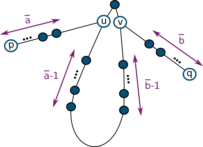
(b) The associated subgraph for Telephone Broadguess

Figure 10: Equivalent Compatible Dome Selection and Telephone Broadcasting Inputs for singleton domes.

We construct the graph $G$ by creating a subgraph for each dome in $\mathcal{D}$, with all subgraphs sharing a common root vertex $r$, referred to as the center. The construction of each subgraph depends on the dome type, whether it is a singleton dome or a regular dome.

The subgraph for a singleton dome $(a,b)$ is constructed as follows. Start with a path of $\overline{a}+\overline{b}$ vertices, labeling the first vertex as $u$ and the last as $v$. Attach a path of $\overline{a}$ vertices to $u$, with its last vertex labeled as $p$. Similarly, attach a path of $\overline{b}$ vertices to $v$, with its last vertex labeled as $q$. Finally, connect both $u$ and $v$ to $r$ to complete the subgraph. The construction is illustrated in Figure 10.

The subgraph for a regular dome $(a,b,c,d)$ is constructed as follows. Start with a path of $\overline{d}+\overline{b}+1$ vertices, labeling the first vertex as $u$, the last as $v$, and the $(\overline{b}+1)$-th vertex as $z$. Attach a separate path of $\overline{b}$ vertices to $u$, with its last vertex labeled as $p$. Similarly, attach a path of $\overline{d}$ vertices to $v$, with its last vertex labeled as $q$. Additionally, attach $\overline{a}-\overline{b}=\overline{c}-\overline{d}$ nodes directly to $z$. Finally, connect $u$ and $v$ to $r$ to complete the subgraph. The construction is illustrated in Figure 11.

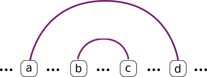
(a) A regular dome in a Compatible Dome Selection instance.

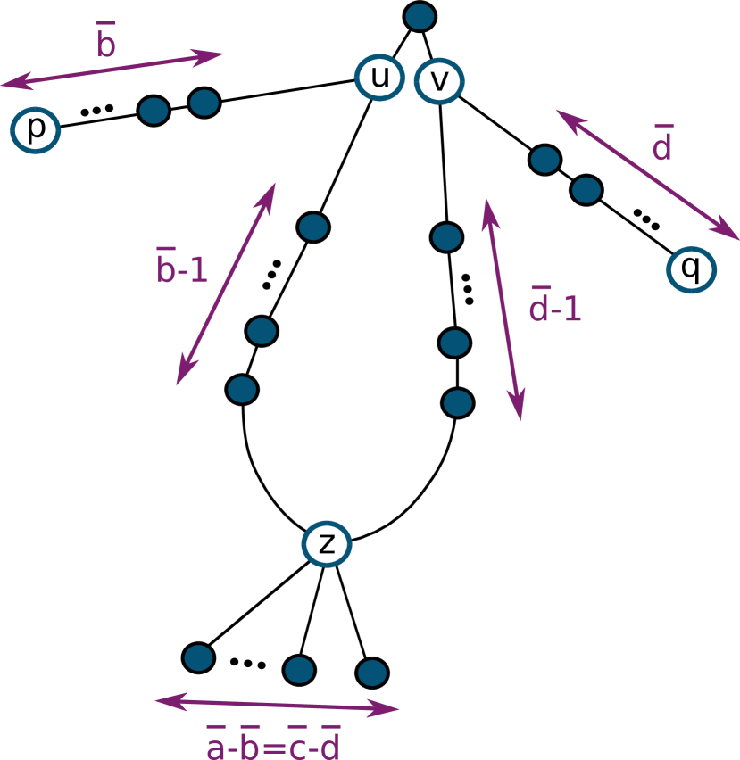
(b) Associated subgraph for Telephone Broadguess.

Figure 11: Equivalent Compatible Dome Selection and Telephone Broadguess instances for regular domes

Based on the construction, every two subgraphs mentioned above have exactly one vertex in common, which is the center. Furthermore, every subgraph has exactly one cycle. Thus, the final graph is a cactus graph. An example of the final snowflake graph after attaching all the subgraphs together is shown in Figure 1. Furthermore, one can readily observe that the size of graph $G$ is polynomial based on $n$ and $m$. Hence, our reduction is polynomial.

4.4.2 Proof of Equivalence

Lemma 4.17.

Given a Compatible Dome Selection instance $\mathcal{D}$ and its corresponding constructed Telephone Broadcasting in snowflake Graph instance $G$, $\mathcal{D}$ has a solution if and only if $G$ can be broadcasted within $\mathcal{B}=2m$ rounds.

Lemma 4.18.

If the Compatible Dome Selection instance $\mathcal{D}$ has a solution, then in the corresponding graph $G$, Telephone Broadcasting can be completed within $\mathcal{B}=2m$ rounds.

Proof. In a valid solution $S$ for Compatible Dome Selection, after selecting an arc from each dome, there is a way to shift them to the left such that the final endpoints of the selected shifted arcs are disjoint. Consider an arc $(a,b)$ is selected from a dome $D$ with its left-shifted version $(x,y)$ such that $x\leq a$ and $y\leq d$. We want to prove that if $r$ informs its two neighbors from the corresponding subgraph of the same dome at rounds $a$ and $b$, the whole subgraph can be informed within $\mathcal{B}$ rounds. Since $x\leq a$ and $y\leq d$, we can inform them at rounds $x$ and $y$ as well and be able to completely broadcast the whole subgraph. As the shifted endpoints in $S$ are distinct, $r$ can inform each subtree with the selected endpoints of its corresponding dome in $S$. This means $G$ can be informed within $\mathcal{B}$ rounds. The proof is divided into two cases based on the dome type.

Case 1: Regular domes.

By definition, we know that $\overline{a}>\overline{b}>\overline{c}>\overline{d}$. Thus, for instance, having $\overline{c}$ remaining rounds is enough to broadcast a path of length $\overline{d}$.

Assuming that the arc $(b,c)$ is selected, nodes $u$ and $v$ have $\overline{b}$ and $\overline{c}$ remaining rounds to broadcast the subgraph, respectively. The node $v$ is responsible for broadcasting up to the node $z$ and its attached nodes. It informs its neighbor in the main cycle in the first round and its neighbor in the path to $q$ in the second round, while the previously informed node informs its other neighbor in the main path. By continuing the broadcasting simultaneously in the main cycle and the attached path, after $(\overline{d}-1)+1+(\overline{c}-\overline{d})=\overline{c}$ rounds, all the nodes of the path up to $q$ (since $\overline{c}>\overline{d}$) and the nodes in the main cycle up to $z$ and its attached nodes are informed. Similarly, node $u$, by first informing its neighbor in the path to $p$ and then its neighbor in the main cycle, and continuing to broadcast simultaneously, can broadcast the path attached to $u$ and the main cycle up to $z$ in $\overline{b}$ rounds. This procedure is illustrated in Figure 12.

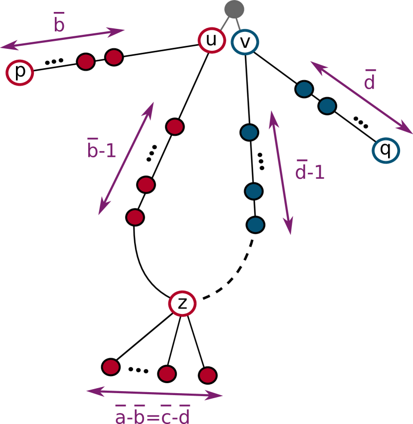
(a) By selecting the arc $(b,c)$, nodes $u$ and $v$ have $\bar{b}$ and $\bar{c}$ remaining broadcast rounds, respectively. Thus, node $v$ is responsible for continuing the broadcast until it reaches node $z$ and its associated subgraph, highlighted in red, while node $u$ is responsible for broadcasting the left side of the subgraph, highlighted in blue.

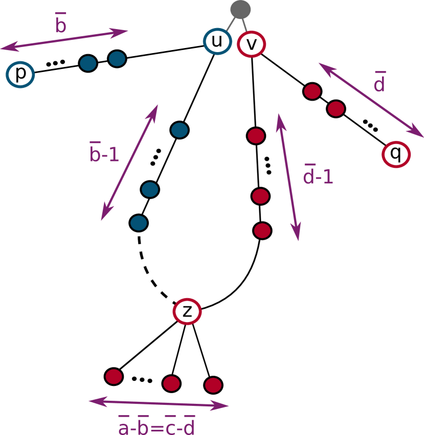
(b) By selecting the arc $(a,d)$, nodes $u$ and $v$ have $\bar{a}$ and $\bar{d}$ remaining broadcast rounds, respectively. Thus, node $u$ is responsible for continuing the broadcast until it reaches node $z$ and its associated subgraph, highlighted in red, while node $v$ is responsible for broadcasting the right side of the subgraph, highlighted in blue.

Figure 12: Two cases of selecting an arc in Compatible Dome Selection and the corresponding broadcasting scheme in Telephone Broadguess are presented.

Similarly, with the arc $(a,d)$ being selected, the node $u$ is responsible for first informing the neighbor in the main cycle and then the neighbor on the path to $p$, broadcasting simultaneously until reaching $z$ and broadcasting its attached nodes all in $\overline{a}$ rounds. The node $v$ can inform the path to $q$ and nodes of the main cycle until $z$ in $\overline{d}$ rounds. This procedure is illustrated in Figure 12. Thus, in both cases, the corresponding subgraph can be broadcasted within the specified rounds.

Case 2: Singleton domes.

Having only one arc $(a,b)$, nodes $u$ and $v$ have $\overline{a}$ and $\overline{b}$ remaining rounds to broadcast the subgraph, respectively. Each of them starts broadcasting to the path attached to it in the first round and broadcasts to the main cycle in the second round, ensuring complete broadcasting within the specified rounds. The procedure is illustrated in Figure 13.

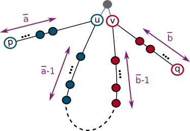
Figure 13: The corresponding broadcast scheme in Telephone Broadguess when there is a singleton dome. The only arc $(a,b)$ is selected, leaving nodes $u$ and $v$ with $\bar{a}$ and $\bar{b}$ remaining broadcast rounds, respectively. Thus, the left side of the subgraph, highlighted in blue, is broadcast by $u$, while the right side, highlighted in red, is broadcast by $v$.

$\Box$

Lemma 4.19.

If Telephone Broadcasting in a graph $G$ can be completed within $\mathcal{B}=2m$ rounds, then the corresponding Compatible Dome Selection instance $\mathcal{D}$ has a solution.

Proof. Consider a solution $S$ that can complete the Telephone Broadcasting in $\mathcal{B}$ rounds. For each subgraph, the center $r$ should inform its two neighbors in the subgraph in two different rounds. We will show that $s$ cannot inform just one of its neighbors from a subgraph and be able to completely broadcast the subgraph.

By definition of Telephone Broadcasting, at each round, we broadcast to only one neighbor of an informed node. Thus, the pairs of rounds in which each subgraph gets informed by $r$ in $S$ are disjoint. In order to prove the same set of pairs works as a solution for the Compatible Dome Selection instance, we need to show that each pair is indeed a left-shifted of one of the arcs of its corresponding dome. The proof is divided into two cases.

Case 1: Regular domes.

Since no dome endpoint can be beyond $m$ in Compatible Dome Selection, for each endpoint $x$, $\overline{x}=\mathcal{B}-x=2m-x\geq m$. Thus, $\overline{b},\overline{d}\geq m$. If we attempt to inform $v$ and sequentially broadcast the main cycle up to $u$, followed by broadcasting the path attached to $u$ up to $p$, it requires at least $(\overline{d}-1)+1+(\overline{b}-1)+1+\overline{b}\geq 3m>\mathcal{B}$, which is not feasible. Therefore, $p$ should be informed via $u$. Similarly, $q$ should be informed via $v$. The same rule applies to the subgraph constructed by singleton domes.

Let the rounds that $r$ informs nodes $u$ and $v$ be $x$ and $y$, respectively. As $u$ should inform $p$, $\overline{x}\geq\overline{b}$. Similarly, $\overline{y}\geq\overline{d}$. $z$ should be informed by either $v$ or $u$, and after that, $\overline{a}-\overline{b}=\overline{c}-\overline{d}$ rounds is needed for the broadcasting to complete. Thus, either $\overline{x}\geq(\overline{b}-1)+1+(\overline{a}-\overline{b})=\overline{a}$ or $\overline{y}\geq(\overline{d}-1)+1+(\overline{c}-\overline{d})=\overline{c}$.

In the first case, we have $\overline{x}\geq\overline{a}$ and $\overline{y}\geq\overline{d}$, resulting in $x\leq a$ and $y\leq d$, meaning that $(x,y)$ are the left-shifted version of $(a,d)$. In the second case, we have $\overline{x}\geq\overline{b}$ and $\overline{y}\geq\overline{c}$, resulting in $x\leq b$ and $y\leq c$, meaning that $(x,y)$ are the left-shifted version of $(b,c)$. Thus, in either case, it converts to a valid solution for Compatible Dome Selection.

Case 2: Singleton domes.

Consider the time that the Telephone Broadcasting solution informs nodes $u$ and $v$ as $x$ and $y$, respectively. Using the same approach as in the previous case of regular domes, it follows that $\overline{x}\geq\overline{a}$ and $\overline{y}\geq\overline{b}$, resulting in $x\leq a$ and $y\leq b$, meaning that $(x,y)$ are the left-shifted version of $(a,b)$. Thus, it converts to a valid solution for Compatible Dome Selection.

$\Box$

Proof of Lemma 4.17: Based on Lemma 4.18 and Lemma 4.19, we have established that the Compatible Dome Selection instance $\mathcal{D}$ is satisfiable if and only if we can complete broadcasting in the equivalent Telephone Broadcasting instance $G$ within $\mathcal{B}=2m$ rounds. This completes the proof of equivalence and validates the reduction from Compatible Dome Selection to Telephone Broadcasting. $\Box$

Theorem 4.20.

Telephone Broadcasting problem is NP-complete for snowflake graphs.

Proof. Through a series of reductions outlined in Lemma 4.7, 4.10, 4.14, and 4.17, we have established that Twin Interval Selection, Dome Selection with Prefix Restrictions, Compatible Dome Selection, and Telephone Broadguess are all NP-hard problems.

Telephone Broadcasting in general graphs is known to be in NP [17]. Together, these results establish that the binary version of Telephone Broadcasting (Telephone Broadguess) is NP-complete even when restricted to snowflake graphs. $\Box$

5 Constant-Factor Approximation for Bounded Pathwidth

Graphs with a pathwidth of $1$ are trees, for which the Telephone Broadcasting problem is solvable in polynomial time [7]. For graphs with a pathwidth greater than $1$, the Telephone Broadcasting problem is NP-hard, as established by our proof for snowflake graphs in Section 4. Note that, based on Observation 2.1, snowflake graphs have a pathwidth of $2$.

This section presents a constant-factor approximation for Telephone Broadcasting on graphs with bounded pathwidth. Consider a graph $G$ with source node $s$, where $\mathcal{B}\boldsymbol{r}(G,s)$ represents the optimal broadcasting time starting from $s$ in $G$. We want to demonstrate that the algorithm designed for graphs with bounded pathwidth by Elkin and Kortsarz [6], which achieves a performance ratio of $O\left(\frac{\log n}{\log\mathcal{B}\boldsymbol{r}(G,s)}\right)$, achieves a constant factor approximation for bounded pathwidth. A simple analysis suggests an approximation ratio of $O\left(\frac{\log n}{\log\log n}\right)$. This is because, in the best scenario, each informed node informs one new neighbor per round, resulting in the total number of informed nodes doubling in each step. Therefore, given that all $n$ nodes of the graph should be informed, the broadcasting time for the optimal solution is at least $\log n$.

In order to provide a constant factor approximation, we prove that $\mathcal{B}\boldsymbol{r}(G,s)\geq n^{\epsilon}$, where $n$ is the number of nodes in the graph and $\epsilon$ is a positive constant based on $w$. By combining these results, we conclude that the aforementioned algorithm achieves a performance ratio of $O\left(1/\epsilon\right)$, thereby providing a constant-factor approximation for graphs with bounded pathwidth.

Lemma 5.1.

After removing an arbitrary node $v$ from an arbitrary connected graph $G$, the sum of broadcasting times over the resulting connected components satisfies $\sum_{C_{i}\in G\setminus\{v\}}\mathcal{B}\boldsymbol{r}(C_{i},s_{i})\leq\mathcal{B}\boldsymbol{r}(G,s)(2\mathcal{B}\boldsymbol{r}(G,s)+1)$ for every arbitrary choice of $s$ and $s_{i}$s.

Proof. Based on the definition of $\mathcal{B}\boldsymbol{r}(G,s)$, a broadcasting scheme exists that starts at $s$ and informs the entire graph $G$ within $\mathcal{B}\boldsymbol{r}(G,s)$ rounds. The edges used to broadcast from one node to another form a broadcasting spanning tree as they do not admit any cycle and cover all nodes. In this rooted spanning tree, the node $v$ is used at some point to inform certain subtrees. Denote these subtrees by $S_{j}$ for $j\in[k]$. Additionally, the subtree containing the whole tree except the subtree of $v$ is denoted by $S_{0}$. Note that when $v=s$, $S_{0}$ is an empty set. Thus, when $v$ is removed, the graph is divided into $k+1$ connected subtrees, each with a designated node responsible for broadcasting within its subtree: for $j\in[k]$, the designated node $u_{j}$ is the $j$-th neighbor of $v$ that $v$ informed in the original graph, and for $S_{0}$, it is the original source $s$. Figure 14 provides an example of this process. Here, $k\leq\mathcal{B}\boldsymbol{r}(G,s)$, with $k=\mathcal{B}\boldsymbol{r}(G,s)$ implying that $v$ was the source node $s$, and all other nodes were directly connected to it. This is because $v$, like every other node, has at most $\mathcal{B}\boldsymbol{r}(G,s)$ rounds to inform its neighbors.

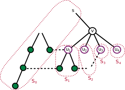
Figure 14: An illustration of the proof of Lemma 5.1. In this example, the sets $S_{0}$ to $S_{4}$ are shown, along with the two connected components formed after removing $v$: one containing $S_{4}$ and the other containing the remaining sets. The designated vertices are shown in purple. Solid edges represent those included in the broadcasting spanning tree, while dotted edges represent those that are not.

Let $C_{i}$ be the $i$-th connected component of $G\setminus\{v\}$. Each connected component may have one or more subtrees $S_{j}$, whose edges are referred to as original edges. To combine the subtrees $S_{j}$ within each component $C_{i}$ into a single spanning tree, incorporate edges from the graph $G$ that were not part of the broadcasting spanning tree. These newly added edges are referred to as auxiliary edges. By combining the original and auxiliary edges, we construct a spanning forest over the connected components $C_{i}$, which is then used to prove the lemma.

We select sources $s_{i}$ for each connected component $C_{i}$, which may not necessarily belong to the set of designated nodes. Considering the original edges, each $s_{i}$ lies within a tree $S_{j}$. To begin, we broadcast along the original edges until reaching the root of $S_{j}$ which is the designated node for $S_{j}$. Since the height of $S_{j}$ is at most $\mathcal{B}\boldsymbol{r}(G,s)$ (as the entire graph $G$ can be broadcasted within this many rounds) broadcasting from $s_{i}$ to $u_{j}$ cannot take more than $\mathcal{B}\boldsymbol{r}(G,s)$ rounds. Next, we broadcast the entire subtree $S_{j}$, which requires an additional $\mathcal{B}\boldsymbol{r}(G,s)$ rounds.

Now, we can use auxiliary edges to inform another subtree $S_{j}^{\prime}$ within the connected component $C_{i}$. After completing the broadcast within the spanning tree $S_{j}^{\prime}$ using the procedure described above with original edges in $2\mathcal{B}\boldsymbol{r}(G,s)$ rounds, we then utilize auxiliary edges to continue broadcasting to other subtrees within the connected component $C_{i}$. Suppose there are $t_{i}$ subtrees in a connected component $C_{i}$. In that case, we require at most $t_{i}-1$ rounds using auxiliary edges to traverse between subtrees, and at most $2\mathcal{B}\boldsymbol{r}(G,s).t_{i}$ rounds to broadcast within each subtree using original edges.

Since there are at most $\mathcal{B}\boldsymbol{r}(G,s)$ non-empty subtrees $S_{j}$ in the graph $G$, it follows that $\sum_{i}t_{i}\leq\mathcal{B}\boldsymbol{r}(G,s)$. For a connected component $C_{i}$, the broadcasting process takes $t_{i}(2\mathcal{B}\boldsymbol{r}(G,s)+1)$ rounds. Summing this across all connected components proves the lemma. $\Box$

Observation 5.1.

Lemma 5.1 is approximately tight for fan graphs.

Proof. A fan graph contains a path of length $n$, where each node in the path is connected to an additional central node $v$. Figure 15 shows the structure of a fan graph.

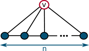
Figure 15: The structure of a fan graph is shown, where the $n$ nodes of the main path, colored in blue, are all connected to a central node $v$.

Starting with $v$ as the source, we have $\mathcal{B}\boldsymbol{r}(G,v)\leq\frac{n}{2\sqrt{n}}+1+\sqrt{n}+1=1.5\sqrt{n}+2$. This is achieved by selecting nodes at positions $1$ and $2i\sqrt{n}$ for $i\in[\sqrt{n}/2]$ along the path to serve as intermediate broadcasting points and broadcasting to them sequentially, followed by $\sqrt{n}+1$ rounds to complete broadcasting along the path from both sides of these nodes. However, $\mathcal{B}\boldsymbol{r}(G\setminus\{v\},s)=n-1$, by setting $s$ to one end of the path and proceeding node by node until reaching the final node of the path. Thus, $\mathcal{B}\boldsymbol{r}(G\setminus\{v\},s)=\Omega(\mathcal{B}\boldsymbol{r}^{2}(G,v))$ demonstrates the tightness of the analysis for fan graphs. $\Box$

Definition 5.2.

A standard path decomposition is a path decomposition in which the nodes in each bag are not a subset of the nodes in the preceding or succeeding bag along the path.

Observation 5.2.

For every arbitrary graph $G$ with pathwidth $w$, there exists a standard path decomposition with pathwidth $w$.

Proof. A path decomposition can always be converted to a standard path decomposition by merging any pair of adjacent bags where one is a subset of the other. This transformation preserves the validity of the path decomposition, as the larger bag covers all the edges of the smaller bag as well. The merging process is repeated until every pair of adjacent bags $A$ and $B$ have non-empty $A-B$ and $B-A$. $\Box$

Lemma 5.3.

For a connected graph $G$ with more than one vertices and bounded pathwidth $w$ and a standard path decomposition of length $\ell$, in which the first bag contains the source vertex $s$, we have $\mathcal{B}\boldsymbol{r}(G,s)\geq 27^{-w}(w!)^{-2}\ell^{4^{-w}}$.

Proof. Consider a standard path decomposition with pathwidth $w$ and length $\ell$. We add an edge between every pair of nodes within the same bag of the standard path decomposition if such an edge does not already exist, ensuring that all node pairs in a bag are directly connected. Adding edges cannot increase the broadcasting time. We demonstrate that the lemma remains valid even with these additional edges.

Let $f(\ell,w)=27^{-w}(w!)^{-2}\ell^{4^{-w}}$ be our lower bound function. First, we generalize the lemma to cover disconnected graphs that do not have any singleton connected component. This change helps prove the lemma using induction. For each connected component $C_{i}$ consider a source vertex $s_{i}$, which is in the leftmost bag of $C_{i}$ in the path decomposition. Note that the set of bags for every two connected components is disjoint as we connect every two vertices in each bag. We want to prove that $\sum_{C_{i}\in G}\mathcal{B}\boldsymbol{r}(C_{i},s_{i})\geq f(\ell,w)$.

We prove it using induction on the size of the graph $G$. The statement is true when $f(\ell,w)<\leq 1$ as the broadcasting time of each non-singleton connected component is greater than $1$. Based on the definition of our lower bound function $f$, it includes all cases where $\ell\leq 3w$. Part of the base of our induction is similar to the step. Thus, we prove both of them together.

If $G$ is not connected, we apply induction to each connected component, assuming the statement holds for smaller-sized graphs, and then sum the results. Each connected component corresponds to a consecutive set of bags in the standard path decomposition of $G\setminus\{v\}$. Since the function $f(\ell,w)$ is sublinear, the sum of the function applied to smaller values $\ell_{i}$ (where $\sum_{i}\ell_{i}=\ell$) is greater than the function applied to the total length $\ell$. Therefore, we have:

$$\sum_{C_{i}\in G}\mathcal{B}\boldsymbol{r}(C_{i},s_{i})\geq\sum_{C_{i}\in G}f(\ell_{i},w)\geq f(\ell,w)$$

In case $G$ is connected, consider the bags in the standard path decomposition containing a particular node. By construction, these bags form a consecutive sequence along the path, referred to as the node span. For the nodes of the first bag, their node spans form a prefix of the bags in the path decomposition. Let the bag span of a bag denote the union of the node span of its nodes. Let $M_{i}$ be the number of bags on the right side of bag $i$ that are in the bag span of bag $i$. Let $M=\max_{i}M_{i}$. We analyze two cases for the value of $M$ to establish the correctness of the induction.

If $M\leq\frac{\ell-1}{f(\ell,w)}$, consider the node newly introduced in the last bag of the standard path decomposition. We aim to calculate the minimum number of rounds required to reach this node from the source node in the first bag. In each round, the algorithm can advance its bag span at most $M$ bags to the right along the standard path decomposition. To reach its bag span to the last bag, which is $\ell-1$ bags away from the first bag, it requires at least $\frac{\ell-1-M}{M}$ broadcasting rounds. And, it needs an additional round to inform the node that is only in the last bag. Since $M\leq\frac{\ell-1}{f(\ell,w)}$, we have

$$\mathcal{B}\boldsymbol{r}(G,s)\geq\frac{\ell-1-M}{M}+1\geq f(\ell,w).$$

If $M>\frac{\ell-1}{f(\ell,w)}$, consider the bag $B_{m}$ with the largest bag span, $M_{m}=M$. There must be a node $v$ in bag $B_{m}$ with a node span of $M$ bags on the right side of $B_{m}$, meaning $v$ appears in $M+1$ consecutive bags (including $B_{m}$) along the standard path decomposition. Let $B_{e}$ be the rightmost bag containing $v$ and the induced subgraph of bags between $B_{m}$ and $B_{e}$ of the path (including $B_{m}$ and $B_{e}$) be denoted as $G_{2}$, which includes all nodes and edges present in these $M+1$ bags. To prove the statement, we prove that it suffices to show that $\mathcal{B}\boldsymbol{r}(G_{2},s_{2})\geq f(\ell,w)+2w$, where $s_{2}$ can be any vertex in $B_{m}$.

Suppose by contradiction that $\mathcal{B}\boldsymbol{r}(G,s)<f(\ell,w)$. It means there is a broadcasting scheme $S$ that can inform the entire graph, including vertices of $G_{2}$ in less than $f(\ell,w)$ rounds. The neighbor set of the vertices before $B_{m}$ is a subset of $B_{m}$ and they are all connected to each other and $v$. Consider a broadcasting scheme as follows. It skips the first rounds of $S$ until it reaches the first vertex of $B_{m}$, let this first vertex be $x$. After that, it informs every other vertex in bag $B_{m}$ in $w$ rounds as they are all connected to each other. Then it continues until it reaches the first vertex of $B_{e}$ and spends another $w$ rounds to inform all vertices in bag $B_{e}$, then it continues $S$ just for $G_{2}$. One can readily notice that this new broadcasting scheme is a valid scheme for $G_{2}$. This is because first, it informs all vertices in $G_{2}$ as $S$ informs all vertices in $G$. Second, each vertex is either in one of the bags $B_{l}$ and $B_{e}$ that gets informed in one of our additional $2w$ rounds, or it is not in the boundaries of $G_{2}$ and should be informed by vertices inside $G_{2}$ by $S$.

Overall the new broadcasting scheme takes less than $f(\ell,w)+2w$ rounds to inform all the vertices of $G_{2}$ starting by $x$, which implies $\mathcal{B}\boldsymbol{r}(G_{2},s_{2})<f(\ell,w)+2w$. This contradiction shows that in order to prove the statement of our induction, we just need to show $\mathcal{B}\boldsymbol{r}(G_{2},s_{2})\geq f(\ell,w)+2w$, for any $s_{2}\in B_{m}$.

Next, we remove the node $v$ from $G_{2}$ and call the resulting graph $G_{3}$. Let $c$ be the number of singleton connected components of $G_{3}$. If $c\geq f(\ell,w)+2$ then we would need at least $f(\ell,w)$ to just inform these singleton connected components and $v$ (except for the two singleton components that might be on the edges of $G_{2}$ (in bags $B_{m}$ and $B_{e}$), and the statement would be true. This is always the case when $w=1$ as after deleting one vertex we remain with singleton connected components. Thus, assuming $c<f(\ell,w)$, we delete all these singleton connected components from $G_{3}$, and call it $G_{4}$. The number of bags in $G_{4}$, called $M^{\prime}$, is at least $M^{\prime}>M-f(\ell,w)-2$ would Since $v$ was present in all bags of $G_{2}$, removing $v$ reduces the pathwidth by one. By the induction hypothesis, we have:

$$\sum_{C_{i}\in G_{4}\setminus\{v\}}\mathcal{B}\boldsymbol{r}(C_{i},s_{i}) \geq f(M^{\prime},w-1).$$

Using Lemma 5.1, we know that:

$$3\mathcal{B}\boldsymbol{r}^{2}(G_{2},s_{2})\geq \mathcal{B}\boldsymbol{r}(G_{2},s_{2})(2\mathcal{B}\boldsymbol{r}(G_{2},s_{2})+1)$$

$$\geq \sum_{C_{i}\in G_{3}\setminus\{v\}}\mathcal{B}\boldsymbol{r}(C_{i},s_{i})=\sum_{C_{i}\in G_{4}\setminus\{v\}}\mathcal{B}\boldsymbol{r}(C_{i},s_{i})$$

$$\implies \mathcal{B}\boldsymbol{r}(G_{2},s_{2})\geq\sqrt{\frac{\sum_{C_{i}\in G_{4}\setminus\{v\}}\mathcal{B}\boldsymbol{r}(C_{i},s_{i})}{3}}\geq\sqrt{\frac{f(M^{\prime},w-1)}{3}}.$$

We also need to prove that $M^{\prime}\geq\sqrt{\ell}$.

$$M^{\prime} >M-f(\ell,w)-2>\frac{\ell-1}{f(\ell,w)}-f(\ell,w)-2\geq\sqrt{\ell}$$

$$\Longleftarrow \frac{\ell-1}{f(\ell,w)}-f(\ell,w)-2\geq\sqrt{\ell}$$

$$\Longleftarrow \frac{\ell-1}{f(\ell,w)}\geq\sqrt{\ell}+f(\ell,w)+2$$

$$\Longleftarrow \ell-1\geq\sqrt{\ell}f(\ell,w)+f^{2}(\ell,w)+2f(\ell,w)$$

$$\Longleftarrow \ell-1\geq 2\ell^{3/4}/27+\ell^{1/2}/27^{2}+2\ell^{1/4}/27$$

$$\Longleftarrow \ell-1\geq\ell^{3/4}/3$$

$$\Longleftarrow \ell\geq 2/3,$$

The last inequality is true except for base cases that were handled before. By substituting $M=\sqrt{\ell}$, we have:

$$\mathcal{B}\boldsymbol{r}(G_{2},s_{2})\geq \sqrt{\frac{f(M^{\prime},w-1)}{3}}\geq\sqrt{\frac{f(\sqrt{\ell},w-1)}{3}}$$

$$\geq \sqrt{\frac{27^{-w+1}\ell^{4^{-w+1}/2}((w-1)!)^{-2}}{3}}$$

$$\geq 3.27^{-w}\ell^{-w}(w!)^{-2}w$$

$$\geq 3w.f(\ell,w)\geq f(\ell,w)-2w$$

Thus, as we discussed before, it implies that $\mathcal{B}\boldsymbol{r}(G,s)\geq f(\ell,w)$ $\Box$

Lemma 5.4.

For a connected graph $G$ with more than one vertices and bounded pathwidth $w$ and a standard path decomposition of length $\ell$, we have $\mathcal{B}\boldsymbol{r}(G,s)\geq 27^{-w}(w!)^{-2}\left(\frac{\ell}{2}\right)^{4^{-w}}$.

Proof. Similar to the proof of Lemma 5.3, we connect every pair of nodes within the same bag of the standard path decomposition by adding edges where they do not already exist. This guarantees that all node pairs in a bag are directly connected. Since adding edges cannot increase the broadcasting time, proving the lemma for this altered graph achieves a lower bound for the original graph as well.

By definition, vertex $s$ should be in a consecutive set of bags in the path decomposition. Let $B_{l}$ and $B_{r}$ be the leftmost and the rightmost bags containing $s$, respectively. Because there are $\ell$ bags in total, either the number of bags after $B_{l}$ or the number of bags before $B_{r}$ should be at least $\ell/2$, including $B_{l}$ and $B_{r}$ themselves. Without loss of generality assume that the number of bags after $B_{l}$, called $\ell^{\prime}$ is at least $\ell/2$.

Let $G^{\prime}$ be the induced graph of all vertices in the bags after $B_{l}$ (including $B_{l}$). First, we prove that $G^{\prime}$ is a connected graph. This is because all the vertices in $G$ that are not in $G^{\prime}$ are the vertices that do not appear in the bags after $B_{l}$. Thus, the neighbor set of such vertices in $G^{\prime}$ is a subset of $B_{l}$. Therefore, as all vertices of $B_{l}$ are already pairwise connected, adding the vertices of $V(G)\setminus V(G^{\prime})$ to $G^{\prime}$ does not reduce the number of connected components. Hence, because $G$ is a connected graph, $G^{\prime}$ has to be connected as well.

Second, based on Lemma 5.3, we know that

$$\mathcal{B}\boldsymbol{r}(G^{\prime},s)\geq 27^{-w}(w!)^{-2}\left(\ell^{\prime}\right)^{4^{-w}}\geq 27^{-w}(w!)^{-2}\left(\frac{\ell}{2}\right)^{4^{-w}}.$$ (5)

As we discussed earlier, the neighbor set of the vertices before $B_{l}$ is a subset of $B_{l}$ and they are all connected to each other and $s$. Suppose by contradiction $\mathcal{B}\boldsymbol{r}(G,s)<27^{-w}(w!)^{-2}\left(\frac{\ell}{2}\right)^{4^{-w}}$. It means there is a broadcasting scheme $S$ that can inform the entire graph which includes vertices of $G^{\prime}$ in less than $27^{-w}(w!)^{-2}\left(\frac{\ell}{2}\right)^{4^{-w}}$ rounds. Consider a broadcasting scheme as follows. It starts with $w$ rounds informing all other vertices in bag $B_{l}$ and then follows the rest of the rounds as the same as $S$ for just the vertices of $G^{\prime}$. Thus, it takes less than $27^{-w}(w!)^{-2}\left(\frac{\ell}{2}\right)^{4^{-w}}$ rounds. Moreover, it informs all the vertices of $G^{\prime}$, this is because after informing bag $B_{l}$, the set of uninformed vertices of $G^{\prime}$ gets completely disconnected from the rest of the uninformed vertices. Thus, $\mathcal{B}\boldsymbol{r}(G^{\prime},s)<27^{-w}(w!)^{-2}\left(\frac{\ell}{2}\right)^{4^{-w}}$, which is a contradiction with Inequality (5). This contradiction proves the lemma. $\Box$

Theorem 5.5.

A polynomial-time algorithm exists for Telephone Broadcasting in graphs with constant pathwidth $w$, achieving an approximation ratio of $O(4^{w})$.

Proof. In the standard path decomposition, each bag contains at most $w+1$ nodes. The number of bags satisfies $\ell\geq\frac{n}{w+1}$ as each node has to be present in at least one bag. Substituting this into Lemma 5.4, we obtain:

$$\mathcal{B}\boldsymbol{r}(G,s)\geq 27^{-w}(w!)^{-2}\left(\frac{n}{2(w+1)}\right)^{4^{-w}}$$ (6)

The approximation ratio of the algorithm introduced by Elkin and Kortsarz [6] is given by $O\left(\log n/\log\mathcal{B}\boldsymbol{r}(G,s)\right)$. Using Inequality (6) and assuming $w\ll n$, we derive:

$$O\left(\frac{\log n}{\log\left(27^{-w}(w!)^{-2}\left(\frac{n}{2(w+1)}\right)^{4^{-w}}\right)}\right) =O\left(\frac{\log n}{\log(27^{-w})+\log((w!)^{-2})+\log\left(\frac{n}{2(w+1)}\right)^{4^{-w}}}\right)$$

$$=O\left(\frac{\log n}{4^{-w}(\log n-\log{2(w+1}))}\right)$$

$$=O(4^{w})$$

$\Box$

6 Concluding Remarks

In this paper, we resolved an open problem by proving the NP-completeness of Telephone Broadcasting for cactus graphs as well as graphs of pathwidth $2$. We also introduced a constant-factor approximation algorithm for graphs of bounded pathwidth and a $2$-approximation algorithm for cactus graphs. As a topic for future work, one may consider improving the approximation factor for graphs of bounded pathwidth or cactus graphs; in particular, it is open whether Polynomial Time Approximation Schemes (PTASs) exist for these graphs. The algorithmic ideas in this work may apply to broadcasting to other families of sparse graphs.

References

- Ben-Moshe et al. [2012] Boaz Ben-Moshe, Amit Dvir, Michael Segal, and Arie Tamir. Centdian computation in cactus graphs. Journal of Graph Algorithms and Applications, 16(2):199–224, 2012.
- Bhabak and Harutyunyan [2015] Puspal Bhabak and Hovhannes A. Harutyunyan. Constant approximation for broadcasting in k-cycle graph. In Proceedings of first Conference of Algorithms and Discrete Applied Mathematics (CALDAM), volume 8959, pages 21–32, 2015.
- Čevnik and Žerovnik [2017] Maja Čevnik and Janez Žerovnik. Broadcasting on cactus graphs. Journal of Combinatorial optimization, 33:292–316, 2017.
- Ehresmann [2021] Anne-Laure Ehresmann. Approximation algorithms for broadcasting in flower graphs. Master’s thesis, Concordia University, 2021.
- Elkin and Kortsarz [2002] Michael Elkin and Guy Kortsarz. Combinatorial logarithmic approximation algorithm for directed telephone broadcast problem. In Proceedings of the thiry-fourth annual ACM symposium on Theory of computing, pages 438–447, 2002.
- Elkin and Kortsarz [2006] Michael Elkin and Guy Kortsarz. Sublogarithmic approximation for telephone multicast. Journal of Computer and System Sciences, 72(4):648–659, 2006.
- Fraigniaud and Mitjana [2002] Fraigniaud and Mitjana. Polynomial-time algorithms for minimum-time broadcast in trees. Theory of Computing Systems, 35(6):641–665, 2002.
- Grigni and Peleg [1991] Michelangelo Grigni and David Peleg. Tight bounds on minimum broadcast networks. SIAM Journal on Discrete Mathematics, 4(2):207–222, 1991.
- Harutyunyan and Maraachlian [2007] Hovhannes Harutyunyan and Edward Maraachlian. Linear algorithm for broadcasting in unicyclic graphs. In Proceedings of the 13th Annual International Conference on Computing and Combinatorics, pages 372–382, 2007.
- Harutyunyan and Liestman [2001] Hovhannes A Harutyunyan and Arthur L Liestman. Improved upper and lower bounds for k-broadcasting. Networks: An International Journal, 37(2):94–101, 2001.
- Harutyunyan and Maraachlian [2008] Hovhannes A Harutyunyan and Edward Maraachlian. On broadcasting in unicyclic graphs. Journal of combinatorial optimization, 16:307–322, 2008.
- Harutyunyan et al. [2023] Hovhannes A Harutyunyan, Narek Hovhannisyan, and Edward Maraachlian. Broadcasting in chains of rings. In Proceedings of the Fourteenth International Conference on Ubiquitous and Future Networks, pages 506–511, 2023.
- Hedetniemi et al. [1988] Sandra M Hedetniemi, Stephen T Hedetniemi, and Arthur L Liestman. A survey of gossiping and broadcasting in communication networks. Networks, 18(4):319–349, 1988.
- Kortsarz and Peleg [1995] Guy Kortsarz and David Peleg. Approximation algorithms for minimum-time broadcast. SIAM Journal on Discrete Mathematics, 8(3):401–427, 1995.
- Robertson and Seymour [1983] Neil Robertson and Paul D Seymour. Graph minors. i. excluding a forest. Journal of Combinatorial Theory, Series B, 35(1):39–61, 1983.
- Shang et al. [2010] Weiping Shang, Pengjun Wan, and Xiaodong Hu. Approximation algorithms for minimum broadcast schedule problem in wireless sensor networks. Frontiers of Mathematics in China, 5:75–87, 2010.
- Slater et al. [1981] Peter J. Slater, Ernest J. Cockayne, and Stephen T. Hedetniemi. Information dissemination in trees. SIAM Journal on Computing, 10(4):692–701, 1981.
- Tale [2024] Prafullkumar Tale. Double exponential lower bound for telephone broadcast. arXiv preprint arXiv:2403.03501, 2024.
- Tovey [1984] Craig A Tovey. A simplified np-complete satisfiability problem. Discrete applied mathematics, 8(1):85–89, 1984.