Quantum entanglement correlations in double quark PDFs

Abstract

Methods from Quantum Information Theory are used to scrutinize quantum correlations encoded in the two-quark density matrix over light-cone momentum fractions $x_{1}$ and $x_{2}$. A non-perturbative three quark model light-cone wavefunction predicts significant non-classical correlations associated with the “entanglement negativity” measure for asymmetric and small quark momentum fractions. We perform one step of QCD scale evolution of the entire density matrix, not just its diagonal (dPDF), by computing collinearly divergent corrections due to the emission of a gluon. Finally, we present first qualitative numerical results for single-step scale evolution of quantum entanglement correlations in double quark PDFs. At a higher $Q^{2}$ scale, the non-classical correlations manifest in the dPDF for nearly symmetric momentum fractions.

I Introduction

Multi parton interactions (MPI) may occur in high energy proton-proton or proton-nucleus collisions whereby two or more partons from the projectile proton undergo a hard scattering off the target. The simplest such MPI process corresponds to double parton scattering which involves double parton distributions (dPDFs) [1, 2, 3, 4]; we refer to ref. [5] for a review of the theory of double parton scattering. A setup for the computation of double parton distributions via lattice QCD has been described in ref. [6]. dPDFs describe the joint distribution of two partons with light-cone (LC) momentum fractions $x_{1}$ and $x_{2}$, respectively, in the proton.

dPDFs provide very interesting insight into parton correlations in the proton. Indeed, a number of authors have concluded that a simple factorized dPDF, lacking correlations when $x_{1}+x_{2}<1$, of the form

$$f_{ij}(x_{1},x_{2},Q^{2})=f_{i}(x_{1},Q^{2})\,f_{j}(x_{2},Q^{2})\,\Theta(1-x_{1}-x_{2})$$ (1)

does not provide a good approximation to the full dPDF [1, 2, 3, 7, 8]. Here, $i$ and $j$ denote parton flavors, and it has been assumed that the MPI involve a single hard scale $Q^{2}$, for simplicity. We shall first consider the double quark PDF at a low virtuality $Q_{0}^{2}$ of order a hadronic scale; henceforth $Q_{0}^{2}$ will be omitted from the arguments of the dPDFs. If the dPDF at the initial scale $Q_{0}^{2}$ lacks correlations then factorization of the dPDF is preserved by QCD evolution. In sec. III we perform a single evolution step towards higher $Q^{2}$ of the entire density matrix including its off-diagonal elements. This provides first qualitative insight into double parton quantum correlations encoded in the density matrix at $Q^{2}>Q_{0}^{2}$.

A variety of initial conditions for dPDFs with correlations have been proposed. The model by Gaunt and Sterling (GS) [2] for the valence quark dPDFs corresponds to

$$f_{ij}(x_{1},x_{2})=f_{i}(x_{1})\,f_{j}(x_{2})\,\frac{(1-x_{1}-x_{2})^{2}}{(1-x_{1})^{2+n}\,(1-x_{2})^{(2+n)}}$$ (2)

with $n=0.5$. It is understood that the support of this function is restricted to $x_{1},x_{2}>0$ and $x_{1}+x_{2}\leq 1$. In this model correlations arise mainly due to the phase space restriction and the dPDF approaches a factorized form as $x_{1}+x_{2}\ll 1$.

Another model (“model II” in [7]) for correlated valence quark dPDFs has been proposed by Broniowski and Arriola (BA)

$$f_{ij}(x_{1},x_{2})=f_{i}(x_{1})\,f_{j}(x_{2})\,\frac{725}{28}\frac{(x_{1}+x_{2})^{2}}{(1-x_{1})(1+6x_{1}+16x_{1}^{2}+6x_{1}^{3}+x_{1}^{4})(1-x_{2})(1+6x_{2}+16x_{2}^{2}+6x_{2}^{3}+x_{2}^{4})}\ .$$ (3)

This model respects the quark number and momentum sum rules. However, here $f_{ij}(x_{1},x_{2})/f_{i}(x_{1})\,f_{j}(x_{2})$ does not vanish as $x_{1}+x_{2}\to 1$.

In passing we mention also ref. [10] who proposed a construction of initial conditions (at a low $Q^{2}$ scale) for double gluon PDFs from single gluon PDFs. Here we focus on quark dPDFs.

Valence double quark PDFs have also been computed in a “bag model” of the proton [11]. In a “rigid bag” approximation the dPDF factorizes and there are no correlations. However, other treatments of the bag do break factorization into single quark PDFs. In the bag model we do not have a simple analytic form of the dPDF like in the two models mentioned above, and so we will not consider it further in this paper. We do note, however, that this model in principle does provide the complete two-quark density matrix including its off-diagonal elements. Hence, it may be possible to distinguish quantum vs. classical correlations using methods similar to those employed here.

Rinaldi et al. have derived double quark distributions from a constituent quark model light-cone wavefunction (LCwf) of the proton [12, 13, 14] by “tracing over” the remaining quark. This way, all sum rules are satisfied by construction. A rather similar approach is presented here. However, our formulation also provides the off-diagonal elements of the two-quark density matrix. While not required for the construction of the dPDF, knowledge of the entire density matrix is needed to determine the nature of correlations, such as quantum vs. classical, by the application of methods from Quantum Information Theory (QIT).

While the present focus is on double quark PDFs as a function of LC momentum fraction, we note that “flavor interference dPDFs” have recently been mentioned in the literature [15]. These correspond to off-diagonal elements of the two-quark density matrix over flavor, analogous to the off-diagonal elements of the two-quark density matrix over $x$ considered here. As already mentioned above, the novel aspect here is to show how specific methods from QIT can be employed to scrutinize the classical vs. quantum nature of double quark correlations.

There has been great interest recently in understanding various aspects of entanglement of quarks and gluons in the proton, initiated primarily by the work of Kharzeev et al. [16, 17, 18] as well as Kovner et al. [19, 20, 9, 21, 22]. Ref. [23], which focuses on the rapidity evolution of the entanglement entropy, provides a list of additional references on this topic. Moreover, Hatta et al. have recently analyzed entanglement of spin and orbital angular momentum degrees of freedom [24, 25].

I.1 Detection of Quantum Correlations

Our goal is to identify specific correlations in the two-quark density matrix (and hence, the dPDF) which cannot arise classically and therefore must be quantum in nature. General information theoretical analysis of correlations is basis-independent and so requires the eigenvalues of the density matrix, meaning that knowledge of the entire matrix, not just its diagonal, is necessary. We will briefly summarize the relevant QIT theory for the sake of completeness.

Given two systems (e.g. quark 1 and quark 2) separately described by density matrices $\rho^{A}$ and $\rho^{B}$ in Hilbert spaces $\mathcal{H}^{A}$ and $\mathcal{H}^{B}$, there are multiple possibilities for the behavior of the combined system. If the subsystems are disjoint, then the total density matrix $\rho=\rho^{A}\otimes\rho^{B}$ is called a product state and clearly has no correlations between the two systems. In the case of two quarks, this corresponds to a factorized dPDF as in (1), however without the kinematic constraint that $x_{1}+x_{2}\leq 1$.

To introduce correlations, we have to create a mixed state as some weighted sum over product states, as the GS and BA dPDFs do in (2) and (3). A special case is a state that can be written as a classical probability distribution over product states

$$\rho^{AB}=\sum_{i}p_{i}\>\rho_{i}^{A}\otimes\rho_{i}^{B}$$ (4)

with $\sum p_{i}=1$, called a separable state. These states exhibit correlations between the two subsystems, but the correlations can be entirely explained classically. Note that the subsystems can be quantum in nature—we are only commenting on the relationships between them. On the other hand, a state which is not separable must have correlations due to quantum entanglement.

Identifying whether or not a given density matrix is separable is known to be NP-hard [26, 27], so there is no known universal test. However, many partial methods [28, 29, 30] have been formulated for use on specific subsets of density matrices.

One standard measure of entanglement is the entanglement entropy [31]. Given a pure bipartite system $\rho^{AB}$ over $\mathcal{H}^{A}\otimes\mathcal{H}^{B}$, we can form a reduced density matrix $\rho^{A}$ by only tracing over $\mathcal{H}^{B}$. The (von Neumann) entanglement entropy is then defined as

$$S_{{\rm vN}}(\rho^{A})=-\text{tr}\,(\rho^{A}\log\rho^{A})\ .$$ (5)

This definition is symmetric over $A$ and $B$; tracing over $\mathcal{H}^{A}$ and calculating $S_{{\rm vN}}(\rho_{B})$ instead will yield the same value. If $S_{{\rm vN}}(\rho_{A})>0$, we conclude that the two subsystems are entangled. In the next section we start from a pure state describing the proton, but then immediately perform a partial trace over all but two degrees of freedom (d.o.f.) to obtain a mixed state $\rho_{x_{1}x_{2},x_{1}^{\prime}x_{2}^{\prime}}$ with $S_{{\rm vN}}>0$. Since our two-quark density matrix is already mixed, we cannot use the entanglement entropy to draw conclusions about the nature of correlations between the LC momentum fractions of the quarks.

Another operation we can perform on the bipartite density matrix $\rho^{AB}$ is to transpose only one of the subsystems $\rho^{B}$; this is called the partial transpose and is written $\rho^{T_{B}}$. The Peres-Horodecki criterion  [32, 33] states that if this partial transpose has any negative eigenvalues, it cannot be separable, and hence must exhibit some quantum correlations. The absolute value of the sum of these negative eigenvalues is called the negativity $\mathcal{N}(\rho)$. This is a partial result since the inverse of the criterion, that $\mathcal{N}(\rho)=0$ implies that $\rho$ is separable, is only true when $\dim(\mathcal{H}^{A}\otimes\mathcal{H}^{B})$ is either $2\times 2$ or $2\times 3$.

Many other computable quantities, such as the coherent information [34], exist to study quantum correlations between subsystems. Nevertheless, we shall rely on the Peres-Horodecki criterion and entanglement negativity in our analysis of double quark PDFs in the proton. In fact, we are mostly interested not in quantifying the overall “degree of entanglement correlations” but rather in investigating how such correlations affect the dPDF. In this regard, working with the partially transposed density matrix is useful because its negative eigenvalues can be “purged” to construct a nearby density matrix with negativity zero from which the corresponding dPDF follows. This is the idea we pursue in the next section.

II Double Quark Parton Distribution for the Three Quark Fock State

II.1 The Three Quark Fock State

The proton state $\left|P\right\rangle$ can be written as a coherent superposition of all possible Fock states multiplied by their respective Fock space amplitudes, the light-cone wavefunctions (LCwf). For moderate momentum fractions $x_{i}\sim 0.1$ and transverse momenta $|\vec{k}_{i}|\sim\Lambda_{\text{QCD}}$, the three valence quark state should dominate and we approximate the light-cone state of the proton by an effective three-quark wavefunction:

$$\left|P\right\rangle=\left|P^{+},P_{\perp}\!\!\>=0\right\rangle=\int_{[0,1]^{3}}[{\rm d}x_{i}]\int[{\rm d}^{2}k_{i}]\ \Psi_{\text{qqq}}(k_{1},k_{2},k_{3})\ \left|k_{1};k_{2};k_{3}\right\rangle$$ (6)

where

$$[{\rm d}x_{i}]=\prod_{i=1\cdots 3}\frac{{\rm d}x_{i}}{2x_{i}}\,\delta\left(1-\sum_{i}x_{i}\right)\ ,\ \ [{\rm d}^{2}k_{i}]=\prod_{i=1\cdots 3}\frac{{\rm d}^{2}k_{i}}{(2\pi)^{3}}\,(2\pi)^{3}\,\delta\left(\sum_{i}\vec{k}_{i}\right)\ ,$$ (7)

and $k_{i}=(x_{i}P^{+},\vec{k}_{i})$ are the three-momenta of the constituent quarks. The spatial wavefunction is symmetric under exchange of any two quarks, $\Psi_{\text{qqq}}(k_{1},k_{2},k_{3})=\Psi_{\text{qqq}}(k_{2},k_{1},k_{3})$ etc. Since our focus is on correlations in momentum space, we will always trace out spin-flavor and color d.o.f. and assume that eq. (6) provides an effective description of the state in momentum space.

To construct the corresponding density matrix we choose basis states of the form

$$\left|\alpha\right\rangle=\frac{1}{16\pi^{3}}\,\frac{\left|x_{1},\vec{k}_{1};x_{2},\vec{k}_{2};x_{3},\vec{k}_{3}\right\rangle}{\sqrt{x_{1}x_{2}x_{3}}}~\longrightarrow~\left<P|\alpha\right>=\frac{\Psi^{*}_{\text{qqq}}(x_{i},\vec{k}_{i})}{2\sqrt{x_{1}x_{2}x_{3}}}\,\delta\!\left(1-\sum x_{i}\right)\delta\!\left(\sum\vec{k}_{i}\right)~.$$ (8)

The density matrix for the proton state is then

$$\rho_{\alpha\alpha^{\prime}}=\frac{\Psi^{*}_{\text{qqq}}(x_{i}^{\prime},\vec{k}_{i}^{\prime})}{2\sqrt{x_{1}^{\prime}x_{2}^{\prime}x_{3}^{\prime}}}\,\frac{\Psi_{\text{qqq}}(x_{i},\vec{k}_{i})}{2\sqrt{x_{1}x_{2}x_{3}}}~,$$ (9)

where the matrix “indices” are $\alpha=\{x_{1},\vec{k}_{1},x_{2},\vec{k}_{2}\}$, $\alpha^{\prime}=\{x_{1}^{\prime},\vec{k}_{1}^{\prime},x_{2}^{\prime},\vec{k}_{2}^{\prime}\}$; it is implied that the r.h.s. is evaluated for $x_{3}=1-x_{1}-x_{2}$ and $\vec{k}_{3}=-\vec{k}_{1}-\vec{k}_{2}$ (and similar for the primed variables). The trace of the density matrix is computed as

$$\text{tr}\,\rho=\int{{\rm d}x_{1}}{{\rm d}x_{2}}\int\frac{{\rm d}^{2}k_{1}}{16\pi^{3}}\frac{{\rm d}^{2}k_{2}}{16\pi^{3}}\,\rho_{\alpha\alpha}=2\int[{\rm d}x_{i}]\,\,\frac{1}{4}\int[{\rm d}^{2}k_{i}]\,\left|\Psi_{\text{qqq}}(x_{i},\vec{k}_{i})\right|^{2}\ .$$ (10)

We can then construct the reduced density matrix for $x_{1}$ and $x_{2}$ by tracing over the remaining degrees of freedom, given by an integral over the quark transverse momenta

$$\rho_{x_{1}x_{2},x_{1}^{\prime}x_{2}^{\prime}}=\frac{1}{4}\int[{\rm d}^{2}k_{i}]\,\rho_{\alpha\alpha^{\prime}}~.$$ (11)

This reduced density matrix, which has non-zero entropy, will be evaluated in sec. II.3 below.

To date the exact light-cone wavefunction of the proton is unknown, of course, as it requires solving the QCD Hamiltonian. Here we employ a simple model due to Brodsky and Schlumpf (BS) [35, 36] where we take

$$\Psi_{\text{qqq}}=N\sqrt{x_{1}x_{2}x_{3}}\ e^{-\mathcal{M}^{2}/2\beta^{2}}\ ,$$ (12)

with $\mathcal{M}^{2}=\sum(\vec{k}_{i}^{2}+m_{q}^{2})/x_{i}$ being the invariant mass squared of the non-interacting three quark system [37]. The parameters $m_{q}=0.26\ \text{GeV}$ and $\beta=0.55\ \text{GeV}$ have been tuned in refs. [35, 36] to reproduce various properties of the proton such as its electromagnetic form factors. The normalization factor $N$ of the LCwf is determined from $\text{tr}\,\rho=1$.

More involved approaches consider various model Hamiltonians with interactions, and the quark model LCwf are then obtained numerically. Ref. [38] has recently studied quark and gluon entanglement in the proton in this way. However, the wavefunctions and density matrices are then available only numerically. For this first exploration of quantum correlations associated with the entanglement negativity measure we consider the simple BS model above.

II.2 Purging Entanglement Negativity with the PEN transformation

The PEN algorithm, introduced and detailed in ref. [39], can be used to remove the negativity of a density matrix. Namely, it takes a density matrix $\rho$ and produces a new density matrix $\rho^{\prime}$ such that $\mathcal{N}(\rho^{\prime})=0$ by replacing all negative eigenvalues of $\rho^{T_{2}}$ with zeroes. In short, after diagonalizing $\rho^{T_{2}}$ the negative eigenvalues are replaced by 0; we then undo the unitary transformation to the eigenbasis of $\rho^{T_{2}}$ and the partial transposition, and finally rescale the matrix by $1/(1+\mathcal{N}(\rho))$ so that $\text{tr}\,\rho^{\prime}=1$. Note that $\rho^{\prime}$ is not guaranteed to be separable, except for small Hilbert spaces where the Peres-Horodecki criterion is sufficient to establish separability. However, since the negative eigenvalues of the partial transpose of $\rho$ are necessarily associated with quantum correlations, these specific correlations must be removed when the associated eigenvalue is sent to zero.

In some low-dimensional cases such as Bell states, where $\rho^{T_{2}}$ features a single non-degenerate negative eigenvalue, $\rho^{\prime}$ is the closest separable state to $\rho$, i.e. a separable Werner state [40]. If $\rho$ is separable to begin with then the PEN transformation reduces to the identity and $\rho^{\prime}=\rho$.

II.3 Leveraging Center of Mass Variables

In this section we construct the reduced density matrix for the LC momentum fraction degrees of freedom of two quarks. The transverse momentum integrals over the BS wavefunction in eq. (11) can be done by hand, yielding

$$\rho_{x_{1}x_{2},x_{1}^{\prime}x_{2}^{\prime}}\sim\frac{\exp\left[-\frac{m_{q}^{2}}{2\beta^{2}}(A_{1}+A_{2}+A_{3})\right]}{A_{1}A_{2}+A_{1}A_{3}+A_{2}A_{3}}$$ (13)

with $A_{i}=\frac{1}{x_{i}}+\frac{1}{x_{i}^{\prime}}$. Recall that $x_{3}$ is not an independent variable, and should be read as shorthand for $1-x_{1}-x_{2}$ (likewise for $x_{3}^{\prime}$). We now have a mixed density matrix with two subsystems for the two valence quark LC momentum fractions.

The denominator $A_{1}A_{2}+A_{1}A_{3}+A_{2}A_{3}$ does not seem readily factorizable into a polynomial in $x_{1}$ times a polynomial in $x_{2}$ on the diagonal, suggesting that this is not a classical dPDF i.e. it cannot be written as a classical mixture of product states. Our goal is to confirm this guess by numerically exhibiting the presence of quantum correlations in the dPDF. If we go about this the naive way, using the PEN algorithm to erase the negativity of $\rho_{x_{1}x_{2},x_{1}^{\prime}x_{2}^{\prime}}$, the resulting density matrix does not respect the kinematic $x_{1}+x_{2}\leq 1$ constraint of the problem and gives an unphysical dDPF. The simple reason for this is that given $x_{1}+x_{2}\leq 1$ and $x_{1}^{\prime}+x_{2}^{\prime}\leq 1$, partial transposition (swapping $x_{2}$ and $x_{2}^{\prime}$) does not necessarily respect these constraints.

The solution is to use center-of-mass (c.o.m.) coordinates that decouple relative and c.o.m. motion, and factorize the constraints of the problem [37]. By finding the dPDF in the c.o.m. variables, using the PEN algorithm on the c.o.m. density matrix, then changing back to our original variables $x_{1}$ and $x_{2}$, we remove negativity while preserving the momentum constraint.

A set of suitable relative light-cone coordinates for three particles constrained to $x_{1}+x_{2}+x_{3}=1$ are [37]

$$\xi=\frac{x_{1}}{x_{1}+x_{2}}\ ,\ \eta=x_{1}+x_{2}\ ,$$ (14)

with $\xi$, $\eta\in[0,1]$. In terms of these variables,

$$2[{\rm d}x_{i}]\,\,\frac{1}{4}[{\rm d}^{2}k_{i}]=\frac{{\rm d}\xi\,{\rm d}\eta}{2\xi(1-\xi)\,2\eta(1-\eta)}\,\,\frac{1}{4}[{\rm d}^{2}k_{i}]~,$$ (15)

and

$$\rho_{\xi\eta,\xi^{\prime}\eta^{\prime}}=\frac{1}{4}\int[{\rm d}^{2}k_{i}]\,\frac{\Psi^{*}_{\text{qqq}}(\xi^{\prime}\eta^{\prime},\eta^{\prime}(1-\xi^{\prime}),1-\eta^{\prime},\vec{k}_{1},\vec{k}_{2},\vec{k}_{3})}{\sqrt{4\eta^{\prime}(1-\eta^{\prime})\xi^{\prime}(1-\xi^{\prime})}}\,\frac{\Psi_{\text{qqq}}(\xi\eta,\eta(1-\xi),1-\eta,\vec{k}_{1},\vec{k}_{2},\vec{k}_{3})}{\sqrt{4\eta(1-\eta)\xi(1-\xi)}}$$ (16)

is the reduced density matrix over the remaining $\xi$, $\eta$ degrees of freedom. It is normalized such that

$$1=\int{\rm d}\xi{\rm d}\eta\,\rho_{\xi\eta,\xi\eta}\ .$$ (17)

So far $\xi$ and $\eta$ are continuous variables on $[0,1]$. In order to evaluate $\rho_{\xi\eta,\xi^{\prime}\eta^{\prime}}$ on a computer and analyze it with information theoretical techniques, we need a finite dimensional matrix. This is achieved by discretizing the unit interval into a finite number of bins of size $\Delta\xi$ and $\Delta\eta$. The discretized density matrix is

$$\tilde{\rho}_{\xi\eta,\xi^{\prime}\eta^{\prime}}={\Delta\xi\,\Delta\eta}\ \rho_{\xi\eta,\xi^{\prime}\eta^{\prime}}\ .$$ (18)

We can then construct the partial transpose $\tilde{\rho}^{T_{2}}$ and numerically calculate the negativity. For the BS light-cone wavefunction, we employed $\Delta\xi=\Delta\eta$ bins of width $\frac{1}{N}$ for $N=20,40,80,160$ and found that $\mathcal{N}(\tilde{\rho}_{\xi\eta,\xi^{\prime}\eta^{\prime}})$ converges to $\sim\!0.035$. This is because as the number $N$ of bins increases, the eigenvalue density of $\tilde{\rho}^{T_{2}}$ asymptotically approaches the form

$$\frac{{\rm d}N_{\lambda}}{{\rm d}\lambda}=\left((N+1)^{2}-\sum_{i=1}^{n}C_{i}\right)\delta(\lambda)+\sum_{i=1}^{n}C_{i}\,\delta(\lambda-\lambda_{i})$$ (19)

where $C_{i}$ is the multiplicity of the nonzero eigenvalue $\lambda_{i}$. There are $N_{\lambda}=(N+1)^{2}$ total eigenvalues of the partial transpose, but all but a few of them remain in a delta function peak at zero. The nonzero eigenvalues do not drift as $N$ changes, so increasing $N$ only increases the resolution for these values. One notable nonzero eigenvalue is $-0.03$ which provides most of the contribution to the negativity of $\tilde{\rho}$.

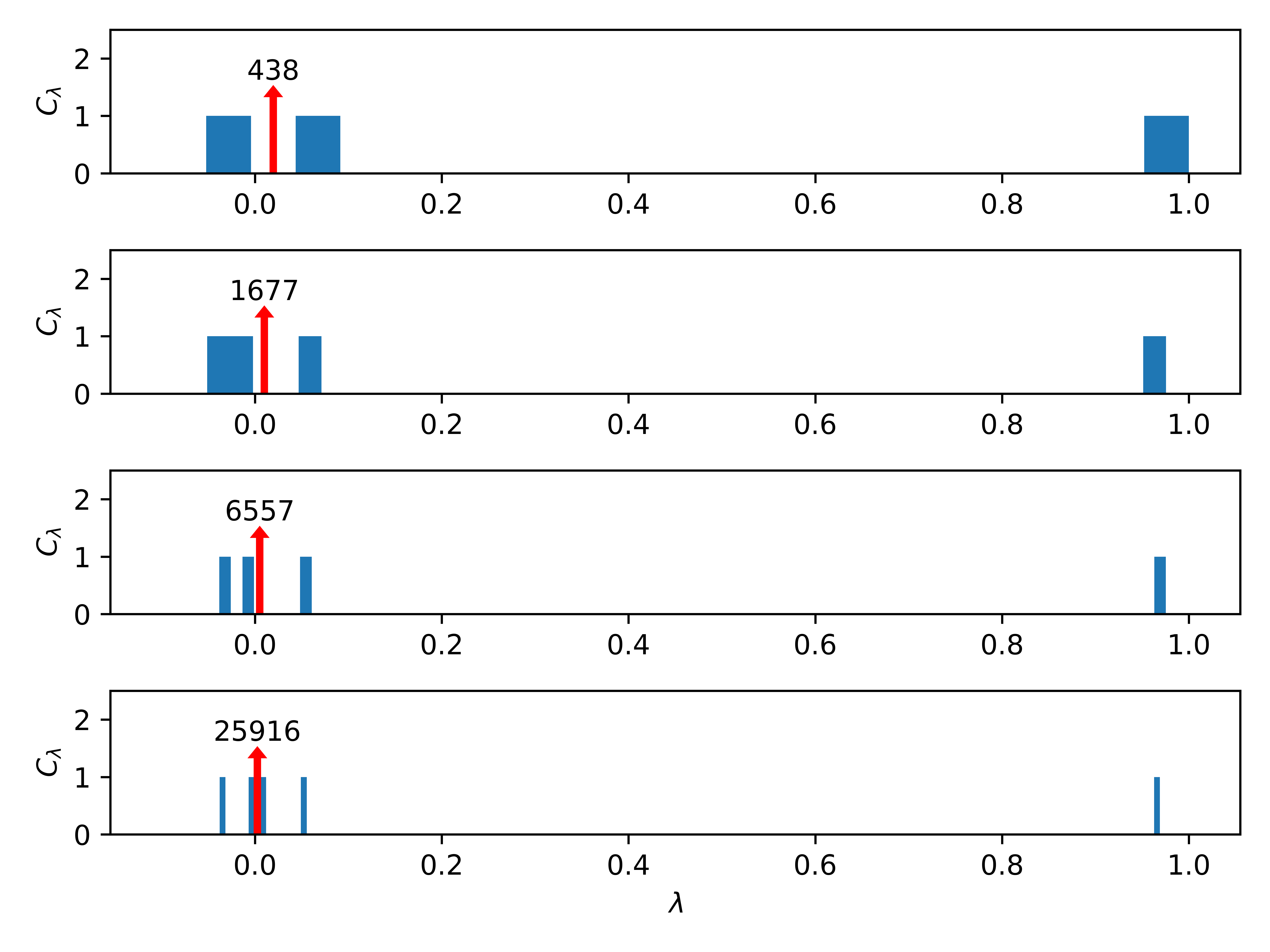
Figure 1: Eigenvalue spectrum of the partial transpose $\tilde{\rho}^{T_{2}}$ for $\frac{1}{\Delta\xi}=\frac{1}{\Delta\eta}=$ 20, 40, 80, 160. The red arrows at the origin signify $\delta(\lambda)$ peaks in the continuum limit. We have chosen to show these peaks as arrows labeled with their correct height, rather than plotting these peaks and obscuring the nonzero eigenvalues.

Once we use the PEN algorithm to purge the negative eigenvalues of the partial transpose, we can return to (discrete) $x_{1}$-$x_{2}$ space for example, to compute single and double PDFs as functions of $x_{1},x_{2}$ as described below.

For the BS light-cone wavefunction, we find the negativity of $\rho_{\xi\eta,\xi^{\prime}\eta^{\prime}}$ to be $\sim\!0.035$. This may be interpreted in the sense that quantum correlations are weak. However, we already mentioned at the end of sec. I.1 that we are mostly interested not in the overall (averaged over momentum fractions) “degree of entanglement”, but in how the presence of quantum correlations affects the dPDF. In the following section we shall see that purging the negativity of the density matrix can result in substantial modification of the dPDF, at least in specific regions of $x_{1}$-$x_{2}$ space.

II.4 Numerical Results for the Quark dPDF

We can compare the structure of the dPDF, both pre- and post-PEN, to models such as the GS model (2) and the BA model (3) by plotting the ratio of the dPDF to the product of two single-quark PDFs,

$$C(x_{1},x_{2})=\frac{f_{qq}(x_{1},x_{2})}{f_{q}(x_{1})\,f_{q}(x_{2})}~.$$ (20)

If the dPDF is simply a product of two single-quark PDFs without any correlations, then this ratio is 1. The dPDF is given by the diagonal elements of the reduced density matrix defined above in eqs. (9, 11),

$$f_{qq}(x_{1},x_{2})=\rho_{x_{1}x_{2},x_{1}x_{2}}~.$$ (21)

This relation can be confirmed by direct computation of the matrix element in the proton state (6) of the operator

$$\frac{\pi\,P^{+}}{(2\pi)^{3}}\,\int{\rm d}^{2}z\int{\rm d}z_{1}^{-}{\rm d}z_{2}^{-}{\rm d}z_{3}^{-}\,e^{-ix_{2}P^{+}(z_{1}^{-}-z_{2}^{-})-ix_{1}P^{+}z_{3}^{-}}O(z_{1}^{-}+\vec{z},z_{2}^{-}+\vec{z})\,O(z_{3}^{-},0)$$ (22)

with $O(z,y)=\bar{q}(z)\gamma^{+}q(y)$, and $q(z)$ the quark field operator at point $z$. (The notation $z^{-}+\vec{z}$ refers to a vector with LC minus component $z^{-}$, and transverse components $\vec{z}$ which represent the transverse spatial separation of the quarks.) In sec. III.3 below we verify that $f_{qq}(x_{1},x_{2})$ satisfies the dPDF DGLAP equation upon emission of a collinear gluon.

The single quark PDF is given by the integral of the dPDF over $x_{2}$ from 0 to $1-x_{1}$,

$$f_{q}(x_{1})=\int\limits_{0}^{1-x_{1}}{\rm d}x_{2}\,f_{qq}(x_{1},x_{2})~.$$ (23)

The dPDF momentum sum rule [2] is satisfied thanks to $f_{qq}(x_{1},x_{2})=f_{qq}(x_{1},1-x_{1}-x_{2})$. We also confirm that $3\int{\rm d}x_{1}\,x_{1}\,f_{q}(x_{1})=2\int[{\rm d}x_{i}]\,(x_{1}+x_{2}+x_{3})\,\frac{1}{4}\int[{\rm d}^{2}k_{i}]\,|\Psi_{\text{qqq}}(x_{1},x_{2},x_{3},\vec{k}_{1},\vec{k}_{2},\vec{k}_{3})|^{2}=\text{tr}\,\rho=1$.

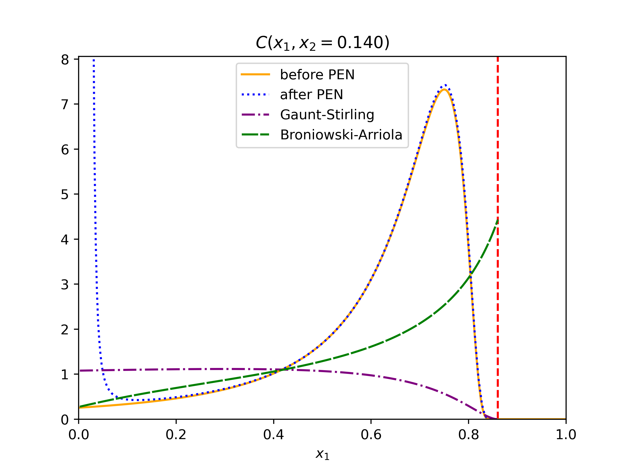
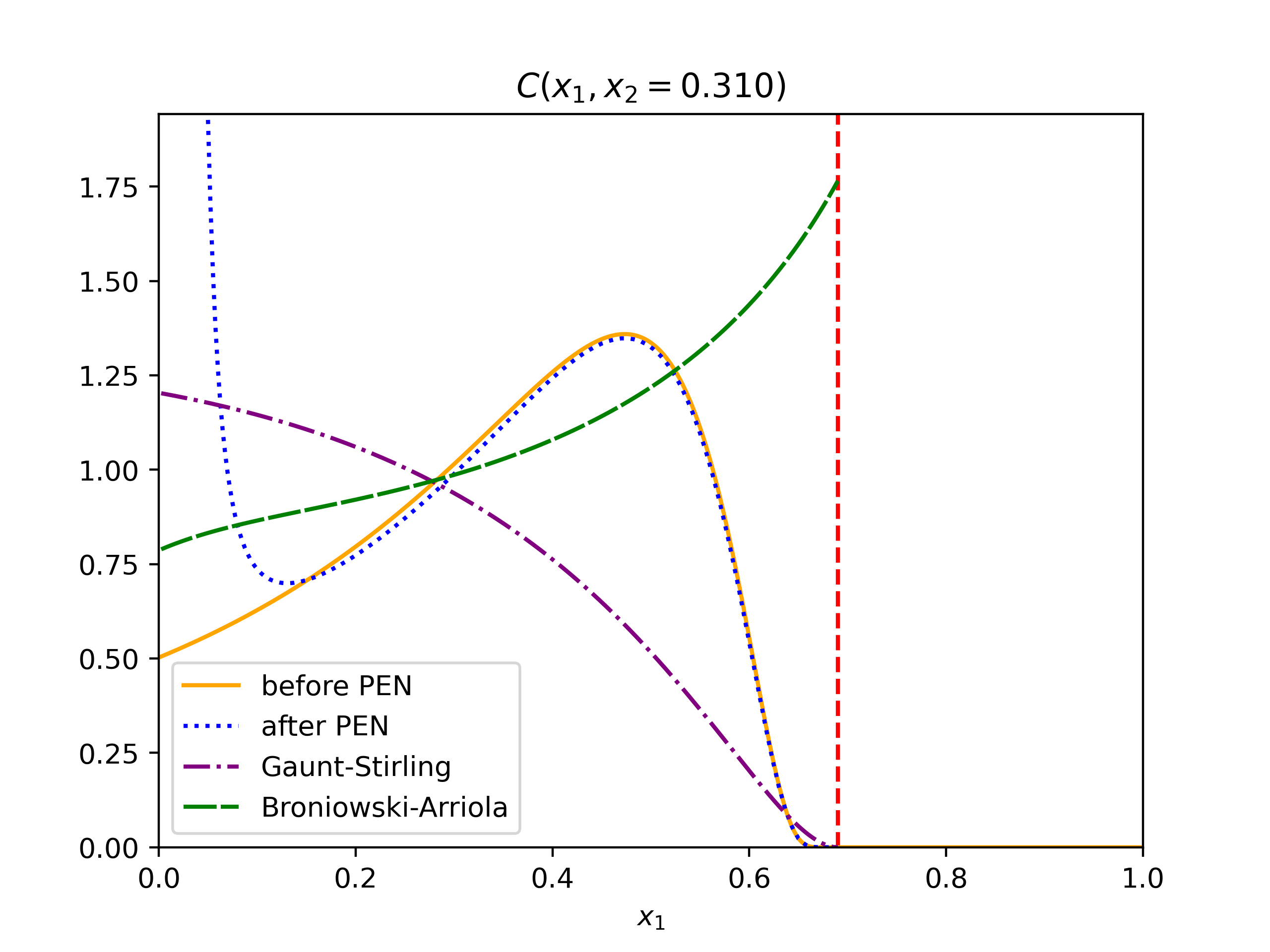
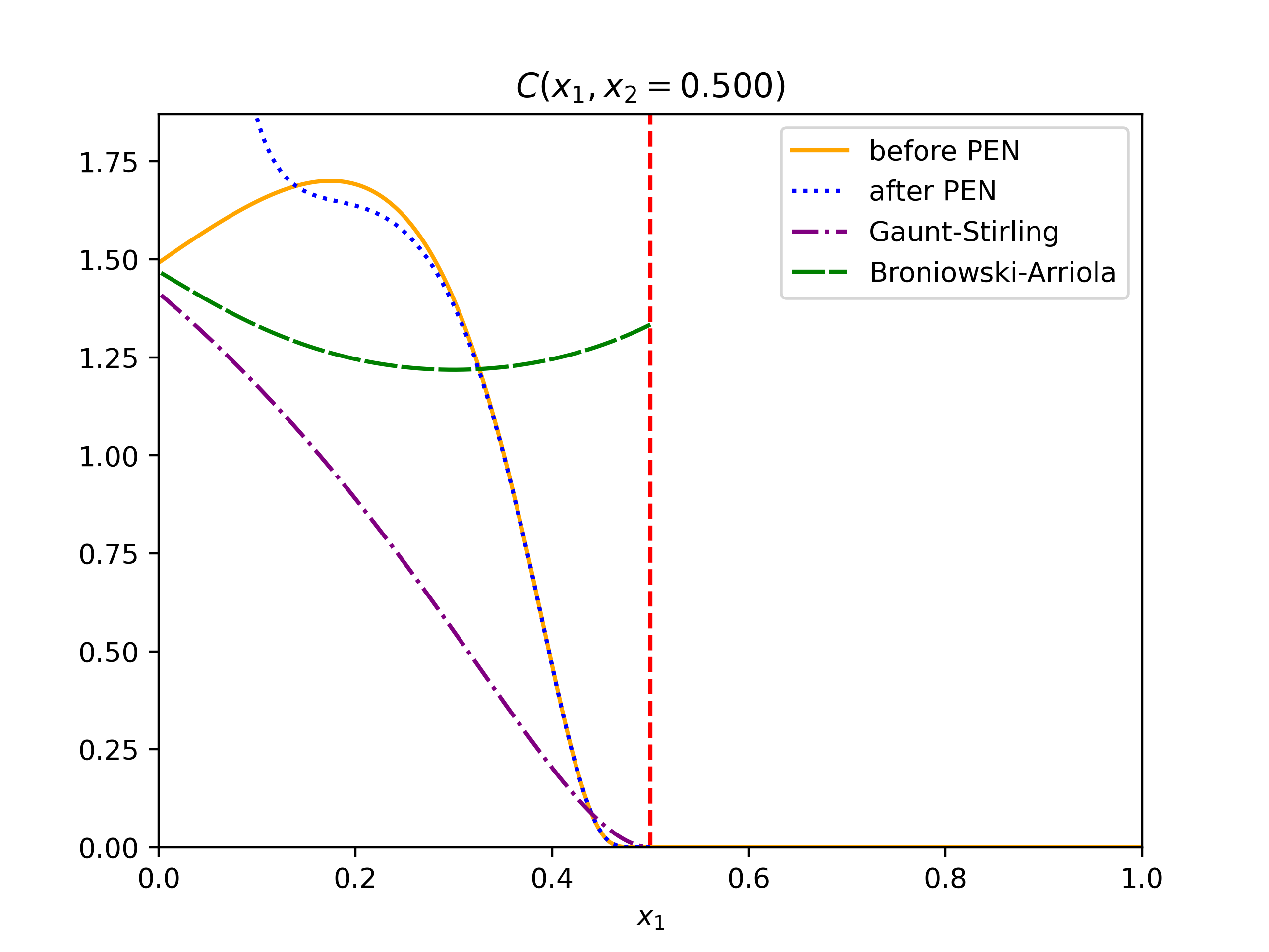
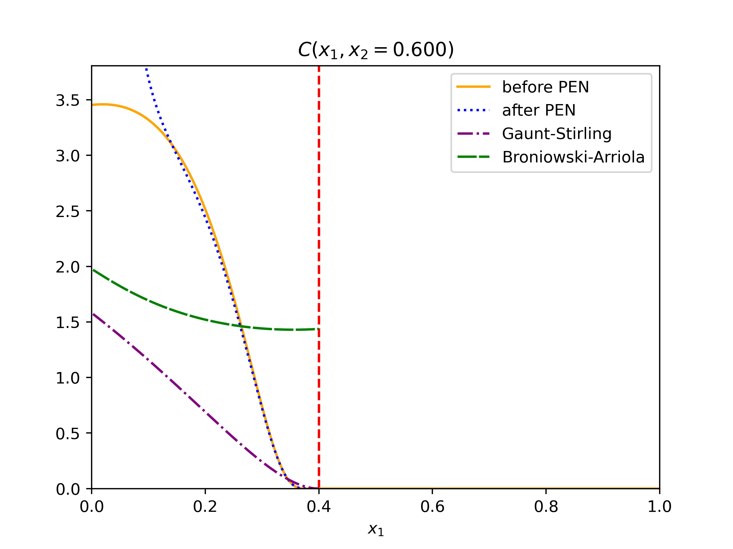
Figure 2: Some selected slices of constant $x_{2}$ for the ratio of the dPDF to the product of two PDFs. The vertical dashed line represents the kinematic boundary where $x_{1}+x_{2}=1$. The dash-dotted and dashed curves correspond to the GS [2] and BA [7] models given in eqs. (2,3), respectively. The solid and dotted curves refer to the dPDF obtained here from the Brodsky-Schlumpf model LCwf [35, 36] before and after the removal of quantum correlations via the PEN algorithm.

Fig. 2 shows $C(x_{1},x_{2})$ as a function of $x_{1}$ for various $x_{2}$. For small $x_{2}=0.14$, the GS model predicts weak correlations up to $x_{1}\approx 0.5$ which then turn into an anti-correlation as the boundary of phase space is approached. The correlation measure obtained from the BS wavefunction is close to the BA model for a large portion of phase space from $x_{1}\sim 0.05$ to $\sim 0.5$; the anti-correlation at small $x_{1}$, $C(x_{1},x_{2})<1$, weakens with increasing $x_{1}$. The BS wavefunction predicts a much stronger correlation for large $x_{1}\simeq 0.7$ but this extreme part of phase space is less relevant in practice. Removal of the quantum correlations associated with negativity (by application of PEN) does not affect the dPDF much when $x_{1}\gtrsim 0.1$ but it does lead to a strong correlation peak at small $x_{1}<0.1$. Hence, assuming that the GS, BA, and the BS LCwf models are close to the real dPDF of QCD we conclude that the LC quark model wavefunction requires the presence of subsystem quantum correlations so as not to strongly overpredict the dPDF at small $x_{2}$, and yet smaller $x_{1}<x_{2}$.

For $x_{2}\simeq 0.3$ we still see fair agreement between the dPDF from the BS wavefunction and the BA model from $x_{1}\sim 0.1$ to $\sim 0.5$. Here, the two qualitatively differ from the GS curve which shows a monotonic decrease and a suppressed dPDF at $x_{1}\geq 0.3$. However, the LC quark model and the GS model both predict a strong suppression of the dPDF towards the edge of phase space, unlike the BA model. We also again observe the appearance of a strong enhancement of the dPDF of the LC quark model at small $x_{1}\leq 0.1$ when the quantum correlations (associated with the negativity measure) of the two quark density matrix are removed.

For the panels in the first row of fig. 2 we may identify the following structure in the BS model. There exists a quantum correlated regime at small $x_{1}<x_{q}^{*}$ where the positive slope of $C(x_{1},x_{2})$ is due to quantum correlations; this regime extends up to about $x_{q}^{*}\approx 0.1$–$0.15$ where the dotted and solid lines merge. Beyond $x_{q}^{*}$, correlations are classical as the dotted and solid lines are on top of each other. However, we can subdivide this further into a classically correlated regime up to $x_{c}^{*}$, which is the point where the curves reach their maximum. In the classically correlated regime between $x_{q}^{*}$ and $x_{c}^{*}$, $C(x_{1},x_{2})$ again exhibits a positive slope. Lastly, beyond $x_{c}^{*}$ we have the cutoff regime where the dPDF drops to 0 very rapidly, faster than the sPDF $f_{q}(x_{1})$, and the slope of $C(x_{1},x_{2})$ is negative. This arises due to the increasing importance of the momentum constraint.

Proceeding to greater $x_{2}=0.5$ we again observe a strong enhancement of the dPDF at small $x_{1}\lesssim 0.2$ due to PEN. This quantum correlated regime then transitions right away into the cutoff regime, i.e. the intermediate classically correlated regime for $x_{q}^{*}<x_{1}<x_{c}^{*}$ has been “squeezed out” by the merging quantum correlated and cutoff regimes.

For $x_{2}=0.6$, the pre- and post-PEN curves exhibit similar behavior. Small phase space suppresses quantum correlations in that both curves exhibit a downward trend. However, the presence of quantum correlations again prevents a stronger enhancement of the dPDF below $x_{1}\sim 0.1$. This is maintained as $x_{2}$ heads towards the upper extreme of phase space.

Summarizing this section, we find that for rather asymmetric momentum fractions $x_{1}$ and $x_{2}$, and well below the kinematic boundary $x_{1}+x_{2}=1$, the BS model LCwf does exhibit significant quantum correlations associated with the negativity measure. On the other hand, for $x_{1}\simeq x_{2}$ or large $x_{1}+x_{2}$, while the dPDF can be substantially different from the product of single quark PDFs, nevertheless these correlations are not associated with entanglement negativity.

III Evolution to Higher Scales

So far we have considered the correlations of the dPDF at a low resolution scale $Q_{0}^{2}$ where a LC quark model may apply. Naturally, one may be interested in how Fig. 2 changes as we evolve to higher scales. The Dokshitzer-Gribov-Lipatov-Altarelli-Parisi (DGLAP) evolution of dPDFs to high $Q^{2}$ has been studied extensively in the literature, see e.g. [1, 2, 3, 4, 5, 7, 8, 10]. However, analysis of classical vs. quantum correlations using negativity and PEN requires knowledge of the entire density matrix, not just the diagonal elements, so we must evolve the entire density matrix. Hence, we require an extension of the dPDF DGLAP equations to off-diagonal density matrix elements. Here we consider only the first step of scale evolution where one of the three valence quarks splits into a quark and a gluon. We consider diagrams which exhibit a collinear divergence. In this section we will use expressions derived in sec. 3 of  [41], and in [42] where the quark wavefunction renormalization factor (virtual corrections) and the Fock space amplitude in LC gauge of the $|qqqg\rangle$ state (real emissions) have been determined.

III.1 Corrections to the density matrix due to one gluon emission

Depending on where we insert our basis states, $\rho_{\alpha\alpha^{\prime}}=\langle P|\alpha\rangle\,\langle\alpha^{\prime}|P\rangle$, we have to consider either a gluon emitted and absorbed by the same quark in $\left|P\right\rangle$ or $\left\langle P\right|$, i.e. a virtual correction, or a “real emission” diagram where a gluon is exchanged by quark $i$ in $\left|P\right\rangle$ and the corresponding quark in $\left\langle P\right|$.

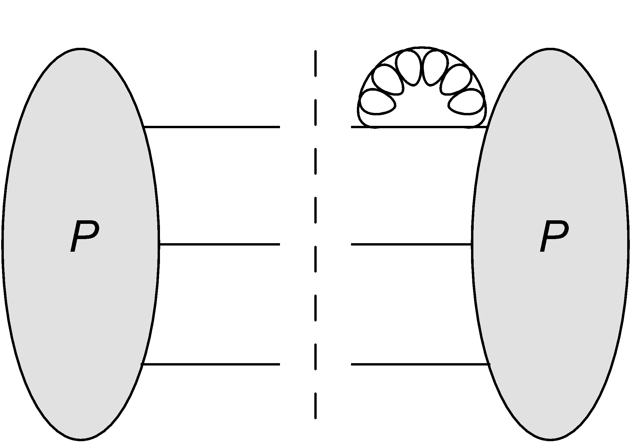
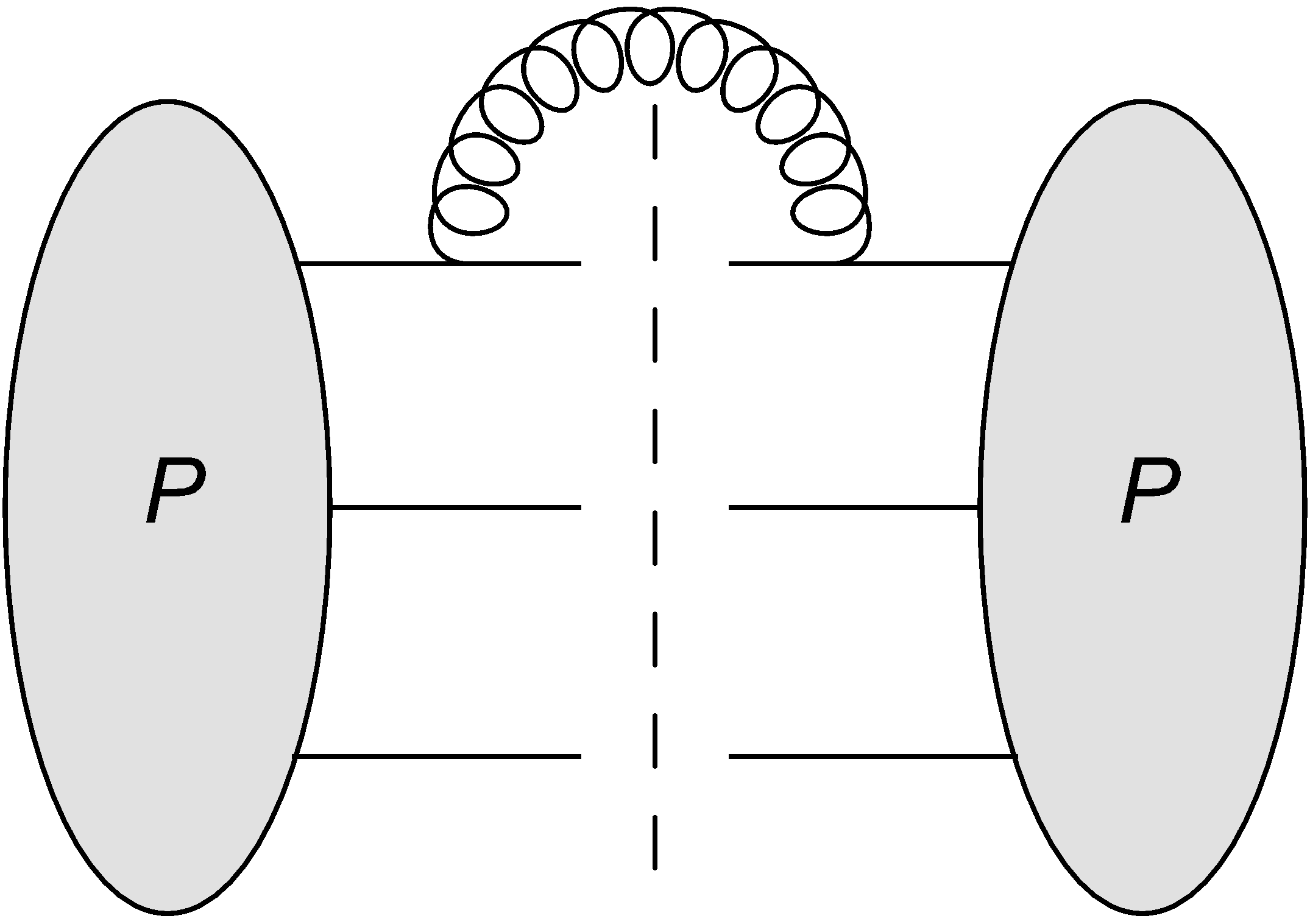
Figure 3: Two diagrams representing, respectively, the emission and absorption of a gluon by quark 1, and the exchange of a gluon between quarks 1’ and 1. The dashed line represents the insertion of two-quark basis states. There are six diagrams of the first type and three of the second type.

The first case gives the quark wavefunction renormalization factor $Z_{q}^{1/2}=(1-C_{q})^{1/2}\simeq 1-C_{q}/2$ via

$$C_{q}\left(x_{i};x,\frac{M_{\text{UV}}}{m_{\text{col}}}\right) =\frac{2g^{2}C_{F}N_{C}}{3}\int_{x}^{1}\frac{{\rm d}x_{g}}{x_{g}}\int\frac{\mathrm{d}^{2}k_{g}}{16\pi^{3}}\ \Theta(x_{i}-x_{g})\left[1+\left(1-z\right)^{2}\right]\left[\frac{1}{k_{g}^{2}+\Delta^{2}}-\frac{1}{k_{g}^{2}+\Lambda^{2}}\right]$$ (24)

$$=\frac{\alpha_{s}}{\pi}C_{F}\,\log\frac{M_{\text{UV}}^{2}}{m_{\text{col}}^{2}}\left[\log\frac{x_{i}}{x}-\frac{(3x_{i}-x)(x_{i}-x)}{4x_{i}^{2}}\right]\,\Theta(x_{i}-x)~.$$ (25)

Here $z=x_{g}/x_{i}$, and $\Delta=zm_{\text{col}}$ where $m_{\text{col}}$ denotes a quark mass regulator for the collinear singularity. $N_{C}=3$ the number of colors in QCD, $C_{F}=(N_{C}^{2}-1)/2N_{C}=4/3$ the quadratic Casimir of the fundamental representation, and $\alpha_{s}=g^{2}/4\pi$ the coupling. The factor $C_{F}[1+\left(1-z\right)^{2}]$ represents, of course, the splitting function $zP_{g\leftarrow q}(z)$.

We have regularized the UV divergence by introducing a cutoff with $\Lambda=zM_{\text{UV}}$, and the soft divergence by a cutoff $x$ on the LC momentum fraction of the gluon. The above expression corresponds to the first step of evolution taking us from the scale $m_{\text{col}}$ to $M_{\text{UV}}$. Since we consider just one single collinear gluon emission we must require that $C_{q}(x_{i})\ll 1$.

The wavefunction renormalization factor arises for each of the six quark lines:

$$\Psi^{*}_{\text{qqq}}(\xi^{\prime},\eta^{\prime},\vec{k}_{i}^{\prime})\,\Psi_{\text{qqq}}(\xi,\eta,\vec{k}_{i}) \rightarrow\Psi^{*}_{\text{qqq}}(\xi^{\prime},\eta^{\prime},\vec{k}_{i}^{\prime})\,\Psi_{\text{qqq}}(\xi,\eta,\vec{k}_{i})\left[1-\frac{1}{2}C_{q}\left(x_{1};x,\frac{M_{\text{UV}}}{m_{\text{col}}}\right)-\frac{1}{2}C_{q}\left(x_{1}^{\prime};x,\frac{M_{\text{UV}}}{m_{\text{col}}}\right)\right.$$

$$\hskip 145.70029pt-\frac{1}{2}C_{q}\left(x_{2};x,\frac{M_{\text{UV}}}{m_{\text{col}}}\right)-\frac{1}{2}C_{q}\left(x_{2}^{\prime};x,\frac{M_{\text{UV}}}{m_{\text{col}}}\right)$$

$$\hskip 145.70029pt-\left.\!\frac{1}{2}C_{q}\left(x_{3};x,\frac{M_{\text{UV}}}{m_{\text{col}}}\right)-\frac{1}{2}C_{q}\left(x_{3}^{\prime};x,\frac{M_{\text{UV}}}{m_{\text{col}}}\right)\right]\ .$$ (26)

Here the $x_{i}$ should be read as shorthands for the associated expressions in terms of $\xi$ and $\eta$ as defined in (14), i.e. $x_{1}=\xi\eta$, $x_{2}=\eta(1-\xi)$, and $x_{3}=1-\eta$. For clarity from now on we shall write the arguments of the three-quark wavefunction in the following order: $\Psi_{\text{qqq}}(x_{1},x_{2},\vec{k}_{1},\vec{k}_{2})$. It is understood that the third LC momentum fraction and transverse momentum is determined by conservation of momentum.

Tracing over the quark transverse momenta $\vec{k}_{i}$ then gives e.g.

$$\rho^{(11)}_{x_{1}x_{2},x_{1}^{\prime}x_{2}^{\prime}} =-\frac{g^{2}C_{F}}{(4\pi)^{2}}\,\log\frac{M_{\text{UV}}^{2}}{m_{\text{col}}^{2}}\,\,\frac{1}{4}\int[{\rm d}^{2}k_{i}]\int_{x}^{1}\frac{{\rm d}x_{g}}{x_{g}}\ \Theta(x_{1}-x_{g})\,\left[1+\left(1-z\right)^{2}\right]\frac{\Psi^{*}_{\text{qqq}}(x_{1}^{\prime},x_{2}^{\prime},\vec{k}_{1},\vec{k}_{2})}{2\sqrt{x_{1}^{\prime}x_{2}^{\prime}x_{3}^{\prime}}}\,\frac{\Psi_{\text{qqq}}(x_{1},x_{2},\vec{k}_{1},\vec{k}_{2})}{2\sqrt{x_{1}x_{2}x_{3}}}$$ (27)

$$=-\frac{g^{2}C_{F}}{(4\pi)^{2}}\,\log\frac{M_{\text{UV}}^{2}}{m_{\text{col}}^{2}}\,\int_{x}^{1}\frac{{\rm d}x_{g}}{x_{g}}\ \Theta(x_{1}-x_{g})\,\left[1+\left(1-z\right)^{2}\right]\,\rho^{\mathrm{qqq}}_{x_{1}x_{2},x_{1}^{\prime}x_{2}^{\prime}}~.$$ (28)

$\rho^{\mathrm{qqq}}_{x_{1}x_{2},x_{1}^{\prime}x_{2}^{\prime}}$ is the non-perturbative reduced density matrix of the three quark state before gluon emission, see sec. II. The trace of this density matrix is computed by setting $x_{1}=x_{1}^{\prime}$, $x_{2}=x_{2}^{\prime}$ and integrating with the measure ${\rm d}x_{1}{\rm d}x_{2}$, as already mentioned in eq. (10). Changing to unconstrained $\xi$, $\eta$ variables,

$$\rho^{(11)}_{\xi\eta,\xi^{\prime}\eta^{\prime}} =-\frac{g^{2}C_{F}}{(4\pi)^{2}}\,\log\frac{M_{\text{UV}}^{2}}{m_{\text{col}}^{2}}\,\,\frac{1}{4}\int[{\rm d}^{2}k_{i}]\int_{x}^{1}\frac{{\rm d}x_{g}}{x_{g}}\,\Theta(\xi\eta-x_{g})\left[1+\left(1-z\right)^{2}\right]$$

$$~~~~~~~~~~~~~\frac{\Psi^{*}_{\text{qqq}}(\xi^{\prime}\eta^{\prime},\eta^{\prime}(1-\xi^{\prime}),\vec{k}_{1},\vec{k}_{2})}{\sqrt{4\eta^{\prime}(1-\eta^{\prime})\xi^{\prime}(1-\xi^{\prime})}}\,\frac{\Psi_{\text{qqq}}(\xi\eta,\eta(1-\xi),\vec{k}_{1},\vec{k}_{2})}{\sqrt{4\eta(1-\eta)\xi(1-\xi)}}~.$$ (29)

The trace of this density matrix is computed by setting $\xi=\xi^{\prime}$, $\eta=\eta^{\prime}$ and integrating with the measure ${\rm d}\xi{\rm d}\eta$, cf. eqs. (15,17). Adding this contribution to $\rho_{\xi\eta,\xi^{\prime}\eta^{\prime}}$ on the r.h.s. of eq. (16) accounts for the ${\cal O}(\alpha_{s}\log{M_{\text{UV}}^{2}}/{m_{\text{col}}^{2}})$ virtual correction.

Now we consider the real emission correction between quarks $i$ and $i^{\prime}$. The four particle density matrix for the $1$ to $1^{\prime}$ gluon exchange (summed over gluon polarizations) is

$$\rho^{(11^{\prime})}_{\text{qqqg}} =\frac{g^{2}}{3}\sum_{m,m^{\prime}}\epsilon_{m^{\prime}n_{2}^{\prime}n_{3}^{\prime}}\,(t^{a^{\prime}})_{m^{\prime}n_{1}^{\prime}}\,\epsilon_{mn_{2}n_{3}}\,(t^{a})_{n_{1}m}\,\Theta(x_{1}-x_{g})\,\Theta(x_{1}^{\prime}-x_{g}^{\prime})$$

$$\hskip 100.00015pt\times\frac{\vec{n}\cdot\vec{n}^{\prime}}{(n^{2}+\Delta^{2})(n^{\prime 2}+\Delta^{\prime 2})}\,(2-z-z^{\prime}+zz^{\prime})\,\frac{\Psi^{*}_{\text{qqq}}(x^{\prime}_{1},x^{\prime}_{2},\vec{k}^{\prime}_{1},\vec{k}^{\prime}_{2})}{2\sqrt{x_{1}^{\prime}x_{2}^{\prime}x_{3}^{\prime}}}\,\frac{\Psi_{\text{qqq}}(x_{1},x_{2},\vec{k}_{1},\vec{k}_{2})}{2\sqrt{x_{1}x_{2}x_{3}}}$$ (30)

with $z=x_{g}/x_{1}$, $\Delta$ defined as before, $\vec{n}=\vec{k}_{g}-z\vec{k}_{1}$, and the primed variables defined analogously. Here we have used the Hilbert space basis introduced in eq. (8).

We need $x_{1}$ to refer to the daughter quark LC momentum when we project onto basis states, so we shift $x_{1}\mapsto x_{1}+x_{g}$. Doing this, then tracing over the gluon color and momentum as well as over the parent quark transverse momenta, yields

$$\rho^{(11^{\prime})}_{x_{1}x_{2},x_{1}^{\prime}x_{2}^{\prime}} ={2g^{2}C_{F}}\,\frac{1}{4}\int[{\rm d}^{2}k_{i}]\int_{x}^{1}\frac{{\rm d}x_{g}}{x_{g}}\,\Theta(1-x_{1}-x_{2}-x_{g})\,\Theta(1-x_{1}^{\prime}-x_{2}^{\prime}-x_{g})\int\frac{\mathrm{d}^{2}k_{g}}{16\pi^{3}}$$

$$\hskip 50.00008pt\times\frac{\vec{n}\cdot\vec{n}^{\prime}}{(n^{2}+\Delta^{2})(n^{\prime 2}+\Delta^{\prime 2})}\,(2-z-z^{\prime}+zz^{\prime})\,\frac{\Psi^{*}_{\text{qqq}}(x_{1}^{\prime}+x_{g},x^{\prime}_{2},\vec{k}_{1},\vec{k}_{2})}{2\sqrt{(x_{1}^{\prime}+x_{g})x_{2}^{\prime}x_{3}^{\prime}}}\,\frac{\Psi_{\text{qqq}}(x_{1}+x_{g},x_{2},\vec{k}_{1},\vec{k}_{2})}{2\sqrt{(x_{1}+x_{g})x_{2}x_{3}}}~,$$ (31)

where now $z=x_{g}/(x_{1}+x_{g})$, $z^{\prime}=x_{g}/(x_{1}^{\prime}+x_{g})$ due to the shifted arguments, and $x_{3}=1-x_{1}-x_{2}-x_{g}$ (and similar for $x_{3}^{\prime}$).

We then introduce the c.o.m. variables $\xi$ and $\eta$ in the same way as in (14) noting that now $x_{3}=1-\eta-x_{g}$ and $\eta<1-x_{g}$. Furthermore,

$$\frac{{\rm d}x_{1}\,{\rm d}x_{2}\,{\rm d}x_{3}}{4(x_{1}+x_{g})x_{2}x_{3}}\,\delta(1-x_{1}-x_{2}-x_{3}-x_{g})=\frac{{\rm d}\xi}{2\xi(1-\xi)}\frac{{\rm d}\eta}{2\eta(1-\eta)}\frac{\Theta(1-\eta-x_{g})}{\left(1+\frac{x_{g}}{\xi\eta}\right)\left(1-\frac{x_{g}}{1-\eta}\right)}$$ (32)

so that

$$\rho^{(11^{\prime})}_{\xi\eta,\xi^{\prime}\eta^{\prime}} ={2g^{2}C_{F}}\,\frac{1}{4}\int[{\rm d}^{2}k_{i}]\int_{x}^{1}\frac{{\rm d}x_{g}}{x_{g}}\frac{\Theta(1-\eta-x_{g})}{\sqrt{\left(1+\frac{x_{g}}{\xi\eta}\right)\left(1-\frac{x_{g}}{1-\eta}\right)}}\,\frac{\Theta(1-\eta^{\prime}-x_{g})}{\sqrt{\left(1+\frac{x_{g}}{\xi^{\prime}\eta^{\prime}}\right)\left(1-\frac{x_{g}}{1-\eta^{\prime}}\right)}}\int\frac{\mathrm{d}^{2}k_{g}}{16\pi^{3}}\frac{\vec{n}\cdot\vec{n}^{\prime}}{(n^{2}+\Delta^{2})(n^{\prime 2}+\Delta^{\prime 2})}$$

$$\hskip 85.00012pt\times(2-z-z^{\prime}+zz^{\prime})\,\frac{\Psi^{*}_{\text{qqq}}(\xi^{\prime}\eta^{\prime}+x_{g},\eta^{\prime}(1-\xi^{\prime}),\vec{k}_{1},\vec{k}_{2})}{\sqrt{4\eta^{\prime}(1-\eta^{\prime})\xi^{\prime}(1-\xi^{\prime})}}\,\frac{\Psi_{\text{qqq}}(\xi\eta+x_{g},\eta(1-\xi),\vec{k}_{1},\vec{k}_{2})}{\sqrt{4\eta(1-\eta)\xi(1-\xi)}}$$ (33)

with $z=x_{g}/(\xi\eta+x_{g})$, $z^{\prime}=x_{g}/(\xi^{\prime}\eta^{\prime}+x_{g})$. We verify that for $(\xi,\eta)\in(0,1)^{2}$ the arguments of the three-quark wavefunctions do not take unphysical values: $x_{g}<1-\eta$ implies $\xi\eta+x_{g}<(\xi-1)\eta+1<1$.

The previous expression is logarithmically UV divergent and we again introduce a UV regulator as

$$-{g^{2}C_{F}}\,\frac{1}{4}\int[{\rm d}^{2}k_{i}]\int_{x}^{1}\frac{{\rm d}x_{g}}{x_{g}}\frac{\Theta(1-\eta-x_{g})}{\sqrt{\left(1+\frac{x_{g}}{\xi\eta}\right)\left(1-\frac{x_{g}}{1-\eta}\right)}}\,\frac{\Theta(1-\eta^{\prime}-x_{g})}{\sqrt{\left(1+\frac{x_{g}}{\xi^{\prime}\eta^{\prime}}\right)\left(1-\frac{x_{g}}{1-\eta^{\prime}}\right)}}\int\frac{{\rm d}^{2}k_{g}}{16\pi^{3}}\,(2-z-z^{\prime}+zz^{\prime})$$

$$\hskip 60.00009pt\times\left[\frac{1}{n^{2}+\Lambda^{2}}+\frac{1}{n^{\prime 2}+\Lambda^{\prime 2}}\right]\frac{\Psi^{*}_{\text{qqq}}(\xi^{\prime}\eta^{\prime}+x_{g},\eta^{\prime}(1-\xi^{\prime}),\vec{k}_{1},\vec{k}_{2})}{\sqrt{4\eta^{\prime}(1-\eta^{\prime})\xi^{\prime}(1-\xi^{\prime})}}\,\frac{\Psi_{\text{qqq}}(\xi\eta+x_{g},\eta(1-\xi),\vec{k}_{1},\vec{k}_{2})}{\sqrt{4\eta(1-\eta)\xi(1-\xi)}}~.$$ (34)

All together we have

$$\rho^{(11^{\prime})}_{\xi\eta,\xi^{\prime}\eta^{\prime}} ={2g^{2}C_{F}}\frac{1}{4}\int[{\rm d}^{2}k_{i}]\int_{x}^{1}\frac{{\rm d}x_{g}}{x_{g}}\,\frac{\Theta(1-\eta-x_{g})}{\sqrt{\left(1+\frac{x_{g}}{\xi\eta}\right)\left(1-\frac{x_{g}}{1-\eta}\right)}}\,\frac{\Theta(1-\eta^{\prime}-x_{g})}{\sqrt{\left(1+\frac{x_{g}}{\xi^{\prime}\eta^{\prime}}\right)\left(1-\frac{x_{g}}{1-\eta^{\prime}}\right)}}(2-z-z^{\prime}+zz^{\prime})\int\frac{\mathrm{d}^{2}k_{g}}{16\pi^{3}}$$

$$\hskip 10.00002pt\times\left[\frac{\vec{n}\cdot\vec{n}^{\prime}}{(n^{2}+\Delta^{2})(n^{\prime 2}+\Delta^{\prime 2})}-\frac{1}{2}\frac{1}{n^{2}+\Lambda^{2}}-\frac{1}{2}\frac{1}{n^{\prime 2}+\Lambda^{\prime 2}}\right]\frac{\Psi^{*}_{\text{qqq}}(\xi^{\prime}\eta^{\prime}+x_{g},\eta^{\prime}(1-\xi^{\prime}),\vec{k}_{1},\vec{k}_{2})}{\sqrt{4\eta^{\prime}(1-\eta^{\prime})\xi^{\prime}(1-\xi^{\prime})}}\,\frac{\Psi_{\text{qqq}}(\xi\eta+x_{g},\eta(1-\xi),\vec{k}_{1},\vec{k}_{2})}{\sqrt{4\eta(1-\eta)\xi(1-\xi)}}~.$$ (35)

At this point we pause to verify that the trace of the density matrix is not only independent of the collinear and UV ($m_{\text{col}}$, $M_{\text{UV}}$) and soft ($x$) cutoffs but, in fact, that the ${\cal O}(\alpha_{s})$ correction cancels altogether so as to preserve the normalization $\text{tr}\,\,\rho=1$.

To compute the trace of (35) we set $\xi^{\prime}=\xi$, $\eta^{\prime}=\eta$, and integrate over ${{\rm d}\xi}{{\rm d}\eta}$. We can then proceed in two ways. First, we can use eq. (32) in reverse thereby also replacing $\xi\eta\to x_{1}$, $\eta(1-\xi)\to x_{2}$, implying $1-\eta-x_{g}\to x_{3}$. We then undo the shift of $x_{1}$ by letting $x_{1}\to x_{1}-x_{g}$ which also introduces a $\Theta(x_{1}-x_{g})$ function. The resulting expression cancels (at leading logarithmic accuracy, up to power corrections) the trace of $\rho^{(11)}$ from eq. (28) plus the same contribution from the trace of $\rho^{(1^{\prime}1^{\prime})}$.

Alternatively, we can also verify the cancellation of the integrals for $\text{tr}\,\rho^{(11^{\prime})}+\text{tr}\,\rho^{(11)}+\text{tr}\,\rho^{(1^{\prime}1^{\prime})}$ in the $\xi,\eta$ variables. In $\text{tr}\,\rho^{(11^{\prime})}$ we perform the transformation

$$\tilde{\eta}=\eta+x_{g}~~,~~\tilde{\xi}=\frac{\xi\eta+x_{g}}{\eta+x_{g}}$$ (36)

so that $1-\eta-x_{g}=1-\tilde{\eta}$, $\eta(1-\xi)=\tilde{\eta}(1-\tilde{\xi})$, and $\xi\eta+x_{g}=\tilde{\xi}\tilde{\eta}$ (similar for the primed variables). This gives rise to a factor $\Theta(\tilde{\xi}\tilde{\eta}-x_{g})$, which allows us to extend the range of both $\tilde{\xi}$ and $\tilde{\eta}$ to $[0,1]$, and restores $z=x_{g}/\tilde{\xi}\tilde{\eta}$ as well as $\Psi_{\text{qqq}}(\xi\eta+x_{g},\eta(1-\xi),\vec{k}_{1},\vec{k}_{2})=\Psi_{\text{qqq}}(\tilde{\xi}\tilde{\eta},\tilde{\eta}(1-\tilde{\xi}),\vec{k}_{1},\vec{k}_{2})$. Furthermore,

$$\frac{{\rm d}\eta\,{\rm d}\xi}{2\xi(1-\xi)\,2\eta(1-\eta)}\frac{1}{\left(1+\frac{x_{g}}{\xi\eta}\right)\left(1-\frac{x_{g}}{1-\eta}\right)}=\frac{{\rm d}\tilde{\eta}\,{\rm d}\tilde{\xi}}{2\tilde{\xi}(1-\tilde{\xi})\,2\tilde{\eta}(1-\tilde{\eta})}$$ (37)

Thus, we again obtain that the trace of eq. (35) cancels against $\text{tr}\,\rho^{(11)}$ (plus the same contribution from $\text{tr}\,\rho^{(1^{\prime}1^{\prime})}$).
  

We now continue our computation with the contribution from the $2$ to $2^{\prime}$ gluon exchange. Here we shift $x_{2}\to x_{2}+x_{g}$ so that $x_{2}$ now corresponds to the LC momentum fraction of daughter quark 2. The measure changes as

$$\frac{{\rm d}x_{1}\,{\rm d}x_{2}\,{\rm d}x_{3}}{4x_{1}(x_{2}+x_{g})x_{3}}\,\delta(1-x_{1}-x_{2}-x_{3}-x_{g})=\frac{{\rm d}\xi}{2\xi(1-\xi)}\frac{{\rm d}\eta}{2\eta(1-\eta)}\,\frac{\Theta(1-\eta-x_{g})}{\left(1+\frac{x_{g}}{(1-\xi)\eta}\right)\left(1-\frac{x_{g}}{1-\eta}\right)}~.$$ (38)

Then

$$\rho^{(22^{\prime})}_{\xi\eta,\xi^{\prime}\eta^{\prime}} ={2g^{2}C_{F}}\frac{1}{4}\int[{\rm d}^{2}k_{i}]\int_{x}^{1}\frac{dx_{g}}{x_{g}}\int\frac{\mathrm{d}^{2}k_{g}}{16\pi^{3}}\,\frac{\Theta(1-\eta-x_{g})}{\sqrt{\left(1+\frac{x_{g}}{(1-\xi)\eta}\right)\left(1-\frac{x_{g}}{1-\eta}\right)}}\,\frac{\Theta(1-\eta^{\prime}-x_{g})}{\sqrt{\left(1+\frac{x_{g}}{(1-\xi^{\prime})\eta^{\prime}}\right)\left(1-\frac{x_{g}}{1-\eta^{\prime}}\right)}}(2-z-z^{\prime}+zz^{\prime})$$

$$\hskip 10.00002pt\times\left[\frac{\vec{n}\cdot\vec{n}^{\prime}}{(n^{2}+\Delta^{2})(n^{\prime 2}+\Delta^{\prime 2})}-\frac{1}{2}\frac{1}{n^{2}+\Lambda^{2}}-\frac{1}{2}\frac{1}{n^{\prime 2}+\Lambda^{\prime 2}}\right]\,\frac{\Psi^{*}_{\text{qqq}}(\xi^{\prime}\eta^{\prime},\eta^{\prime}(1-\xi^{\prime})+x_{g},\vec{k}_{1},\vec{k}_{2})}{\sqrt{4\eta^{\prime}(1-\eta^{\prime})\xi^{\prime}(1-\xi^{\prime})}}\,\frac{\Psi_{\text{qqq}}(\xi\eta,\eta(1-\xi)+x_{g},\vec{k}_{1},\vec{k}_{2})}{\sqrt{4\eta(1-\eta)\xi(1-\xi)}}\ ,$$ (39)

where now $z=x_{g}/(\eta(1-\xi)+x_{g})$, $z^{\prime}=x_{g}/(\eta^{\prime}(1-\xi^{\prime})+x_{g})$, $\vec{n}=\vec{k}_{g}-z\vec{k}_{2}$, and $\Delta$, $\Lambda$ and the corresponding primed variables defined as before. For this contribution the transformation

$$\tilde{\eta}=\eta+x_{g}~~,~~\tilde{\xi}=\frac{\xi\eta}{\eta+x_{g}}~,$$ (40)

which corresponds to $\tilde{\xi}\tilde{\eta}=\xi\eta$, $\tilde{\eta}(1-\tilde{\xi})=\eta(1-\xi)+x_{g}$, is useful for checking the cancellation of the perturbative correction to the trace.

Finally, for the gluon exchange from $3$ to $3^{\prime}$, no shift from parent to daughter quark LC momentum is needed as we are interested in the reduced density matrix over quarks $1$ and $2$. The density matrix for this diagram is

$$\rho^{(33^{\prime})}_{\xi\eta,\xi^{\prime}\eta^{\prime}} ={2g^{2}C_{F}}\frac{1}{4}\int[{\rm d}^{2}k_{i}]\int_{x}^{1}\frac{dx_{g}}{x_{g}}\int\frac{\mathrm{d}^{2}k_{g}}{16\pi^{3}}\,\Theta(1-\eta-x_{g})\,\Theta(1-\eta^{\prime}-x_{g})\,(2-z-z^{\prime}+zz^{\prime})$$

$$\hskip 10.00002pt\times\left[\frac{\vec{n}\cdot\vec{n}^{\prime}}{(n^{2}+\Delta^{2})(n^{\prime 2}+\Delta^{\prime 2})}-\frac{1}{2}\frac{1}{n^{2}+\Lambda^{2}}-\frac{1}{2}\frac{1}{n^{\prime 2}+\Lambda^{\prime 2}}\right]\,\frac{\Psi^{*}_{\text{qqq}}(\xi^{\prime}\eta^{\prime},\eta^{\prime}(1-\xi^{\prime}),\vec{k}_{1},\vec{k}_{2})}{\sqrt{4\eta^{\prime}(1-\eta^{\prime})\xi^{\prime}(1-\xi^{\prime})}}\,\frac{\Psi_{\text{qqq}}(\xi\eta,\eta(1-\xi),\vec{k}_{1},\vec{k}_{2})}{\sqrt{4\eta(1-\eta)\xi(1-\xi)}}\ ,$$ (41)

with $z=x_{g}/(1-\eta)$, $z^{\prime}=x_{g}/(1-\eta^{\prime})$. Here the cancellation of the trace against the last line in (26) is seen immediately.

In summary, single step evolution of the three-quark density matrix from the scale $m^{2}_{\text{col}}=Q_{0}^{2}$ to the higher scale $M^{2}_{\text{UV}}=Q^{2}$ is performed by replacing $\Psi^{*}_{\text{qqq}}(\xi^{\prime}\eta^{\prime},\eta^{\prime}(1-\xi^{\prime}),\vec{k}_{1},\vec{k}_{2})\,\Psi_{\text{qqq}}(\xi\eta,\eta(1-\xi),\vec{k}_{1},\vec{k}_{2})$ in (16) by the sum of virtual corrections (26) followed by adding the density matrices (35, 39, 41) for real emissions. Our result applies in the leading $\log M_{\text{UV}}/m_{\text{col}}\gg 1$ approximation when the coupling $\alpha_{s}$ is sufficiently small, and perhaps the cutoff $x$ on the LC momentum fraction of the gluon is sufficiently large, so that the ${\cal O}(\alpha_{s})$ contribution to the wavefunction renormalization factor (25) is small.

III.2 Cancellation of Soft Divergence

In the previous section, we had to introduce a cutoff $x$ on the LC momentum of the gluon to handle the soft divergence. Here we show that this divergence cancels at leading logarithmic accuracy in the sum of real emissions and virtual corrections. Hence, the integration over $x_{g}$ could in principle extend to 0.

The expressions from the previous section simplify greatly when $x_{g}$ is much less than the typical momentum fraction of a quark, $\left\langle x_{\text{q}}\right\rangle$. We then have $z,z^{\prime}\ll 1$. The integral over the gluon transverse momentum $\vec{k}_{g}$ for the virtual correction in eq. (29) becomes

$$\int\frac{\mathrm{d}^{2}k_{g}}{16\pi^{3}}\left(\frac{1}{k_{g}^{2}+\Delta^{2}}-\frac{1}{k_{g}^{2}+\Lambda^{2}}\right)=\frac{1}{(4\pi)^{2}}\log\frac{M_{\text{UV}}^{2}}{m_{\text{col}}^{2}}\ .$$ (42)

For the real exchanges, the softness of the gluon implies that the daughter quark momentum is the same as that of the parent quark. Since $z,z^{\prime}\ll 1$, we have $\vec{n}=\vec{n}^{\prime}=\vec{k}_{g}$ and the integral over the gluon transverse momentum in $\rho^{(11^{\prime})}$ from eq. (35) becomes

$$2\int\frac{\mathrm{d}^{2}k_{g}}{16\pi^{3}}\left[\frac{k_{g}^{2}}{(k_{g}^{2}+\Delta^{2})(k_{g}^{2}+\Delta^{\prime 2})}-\frac{1}{2}\frac{1}{k_{g}^{2}+\Lambda^{2}}-\frac{1}{2}\frac{1}{k_{g}^{2}+\Lambda^{\prime 2}}\right]\ .$$ (43)

Consider now the sum of the gluon exchange between quarks 1 and $1^{\prime}$ plus the corresponding virtual corrections in the small $x_{g}$ limit:

$$\int\frac{\mathrm{d}^{2}k_{g}}{16\pi^{3}}\left[2\left(\frac{k_{g}^{2}}{(k_{g}^{2}+\Delta^{2})(k_{g}^{2}+\Delta^{\prime 2})}-\frac{1}{2}\frac{1}{k_{g}^{2}+\Lambda^{2}}-\frac{1}{2}\frac{1}{k_{g}^{2}+\Lambda^{\prime 2}}\right)-\left(\frac{1}{k_{g}^{2}+\Delta^{2}}-\frac{1}{k_{g}^{2}+\Lambda^{2}}\right)-\left(\frac{1}{k_{g}^{2}+\Delta^{\prime 2}}-\frac{1}{k_{g}^{2}+\Lambda^{\prime 2}}\right)\right]\ .$$ (44)

Note that

$$\frac{2k_{g}^{2}}{(k_{g}^{2}+\Delta^{2})(k_{g}^{2}+\Delta^{\prime 2})}=\frac{1}{k_{g}^{2}+\Delta^{2}}+\frac{1}{k_{g}^{2}+\Delta^{\prime 2}}+\frac{\Delta^{2}+\Delta^{\prime 2}}{2(k_{g}^{2}+\Delta^{2})(k_{g}^{2}+\Delta^{\prime 2})}~.$$ (45)

The last term does not contribute to the leading-log approximation and can be dropped. This results in a cancellation of the bracketed terms in (44), hence we can take $x\to 0$ with no overall soft divergence when considering the sum of these diagrams. No trace over $\xi$ or $\eta$ has been performed here: this cancellation occurs for the entire density matrix, not just the diagonal elements. The calculation is identical for quarks 2 and $2^{\prime}$, and 3 and $3^{\prime}$.

III.3 DGLAP evolution of the diagonal of the density matrix

In this section we obtain expressions for the derivative with respect to $Q^{2}=M_{\text{UV}}^{2}$ of the diagonal elements of the density matrix, i.e. the double quark PDF. These can be expressed in terms of convolutions of splitting functions and dPDFs.

We have from eq. (28), using relations (9,11),

$$Q^{2}\frac{\partial}{\partial Q^{2}}\rho^{(11)}_{x_{1}x_{2},x_{1}x_{2}}=Q^{2}\frac{\partial}{\partial Q^{2}}\rho^{(1^{\prime}1^{\prime})}_{x_{1}x_{2},x_{1}x_{2}}=-\frac{\alpha_{s}}{4\pi}\int\limits^{1}_{x/x_{1}}{\rm d}z\,P_{g\leftarrow q}(z)\,\rho^{\mathrm{qqq}}_{x_{1}x_{2},x_{1}x_{2}}~.$$ (46)

$\rho^{\mathrm{qqq}}_{x_{1}x_{2},x_{1}^{\prime}x_{2}^{\prime}}$ denotes the non-perturbative reduced density matrix obtained from the three quark LCwf before gluon emission, see sec. II. Similarly,

$$Q^{2}\frac{\partial}{\partial Q^{2}}\rho^{(22)}_{x_{1}x_{2},x_{1}x_{2}} =Q^{2}\frac{\partial}{\partial Q^{2}}\rho^{(2^{\prime}2^{\prime})}_{x_{1}x_{2},x_{1}x_{2}}=-\frac{\alpha_{s}}{4\pi}\int\limits^{1}_{x/x_{2}}{\rm d}z\,P_{g\leftarrow q}(z)\,\rho^{\mathrm{qqq}}_{x_{1}x_{2},x_{1}x_{2}}~,$$ (47)

$$Q^{2}\frac{\partial}{\partial Q^{2}}\rho^{(33)}_{x_{1}x_{2},x_{1}x_{2}} =Q^{2}\frac{\partial}{\partial Q^{2}}\rho^{(3^{\prime}3^{\prime})}_{x_{1}x_{2},x_{1}x_{2}}=-\frac{\alpha_{s}}{4\pi}\int\limits^{1}_{\frac{x}{1-x_{1}-x_{2}}}{\rm d}z\,P_{g\leftarrow q}(z)\,\rho^{\mathrm{qqq}}_{x_{1}x_{2},x_{1}x_{2}}~.$$ (48)

Continuing with the real emission corrections,

$$Q^{2}\frac{\partial}{\partial Q^{2}}\rho^{(11^{\prime})}_{x_{1}x_{2},x_{1}x_{2}} =\frac{2\alpha_{s}}{4\pi}\int\limits_{x_{1}/(1-x_{2})}^{x_{1}/(x_{1}+x)}\frac{{\rm d}z}{z}\,P_{g\leftarrow q}(1-z)\,\rho^{\mathrm{qqq}}_{\frac{x_{1}}{z}x_{2},\frac{x_{1}}{z}x_{2}}~,$$ (49)

$$Q^{2}\frac{\partial}{\partial Q^{2}}\rho^{(22^{\prime})}_{x_{1}x_{2},x_{1}x_{2}} =\frac{2\alpha_{s}}{4\pi}\int\limits_{x_{2}/(1-x_{1})}^{x_{2}/(x_{2}+x)}\frac{{\rm d}z}{z}\,P_{g\leftarrow q}(1-z)\,\rho^{\mathrm{qqq}}_{x_{1}\frac{x_{2}}{z},x_{1}\frac{x_{2}}{z}}~,$$ (50)

$$Q^{2}\frac{\partial}{\partial Q^{2}}\rho^{(33^{\prime})}_{x_{1}x_{2},x_{1}x_{2}} =\frac{2\alpha_{s}}{4\pi}\int\limits^{1}_{\frac{x}{1-x_{1}-x_{2}}}{\rm d}z\,P_{g\leftarrow q}(z)\,\rho^{\mathrm{qqq}}_{x_{1}x_{2},x_{1}x_{2}}~.$$ (51)

The last term simply cancels the corresponding virtual corrections.

The expressions above reproduce the standard equations for DGLAP evolution of double quark PDFs with the identification $f_{qq}(x_{1},x_{2})=\rho_{x_{1}x_{2},x_{1}x_{2}}$, which agrees with eq. (21). The standard form of the dPDF DGLAP equations is

$$\partial_{t}f_{qq}(x_{1},x_{2})=\int\limits_{0}^{1-x_{2}}{\rm d}u\,K(x_{1},u)\,f_{qq}(u,x_{2})+\int\limits_{0}^{1-x_{1}}{\rm d}u\,K(x_{2},u)\,f_{qq}(x_{1},u)~,$$ (52)

where $t=\log Q^{2}$. For example, the contribution involving the real emission kernel

$$K_{R}(x,u)=\frac{\alpha_{s}}{2\pi}\frac{1}{u}P_{qq}(x/u)\,\Theta(u-x)$$ (53)

corresponds exactly to the sum of (49, 50). To see this, use the relation $P_{gq}(1-z)=P_{qq}(z)$ and the transformation $u=x_{1}/z$ or $u=x_{2}/z$, and finally send the cutoff $x\to 0$. The virtual corrections serve to ensure conservation of probability.

Hence, the diagonal of the density matrix evolves according to dPDF DGLAP via a convolution with splitting functions, and independently of the off-diagonal elements.

III.4 Numerical Results

In this section we present first qualitative results on the evolution of quantum correlations in the dPDF to higher scales by evaluating the correction to the density matrix due to the emission of one collinear gluon. The full evolution equation would sum multiple parton splitting steps, a more involved task which we defer to future work.

To keep the perturbative correction small we employ an unrealistically small coupling, $\alpha_{s}=0.1$, and a fairly large cutoff $x=0.1$ on the LC momentum fraction of the gluon. The initial scale $Q_{0}$ corresponding to the quark mass regulator $m_{\text{col}}$ is set to the quark mass $m_{q}=0.26\ \text{GeV}$ encoded in the non-perturbative three-quark BS wavefunction presented at the end of sec. II.1. Also, we choose $Q=M_{\text{UV}}=10m_{\text{col}}$.

The computation of the evolved density matrix is numerically very challenging. It requires the evaluation of a seven dimensional integral, e.g. eq. (35), at each of $N^{2}\times N^{2}/2$ entries of the $(\xi,\eta)-(\xi^{\prime},\eta^{\prime})$ symmetric density matrix, where $N$ is the number of bins per variable. We have used the vegas+ v6.2 algorithm [43, 44] to estimate the density matrix with collinear gluon emission corrections. The evolved dPDF, as the diagonal of the density matrix, only requires $N^{2}$ integrations, so we have computed it with $N=100$ bins. On the other hand, studying the effects of the PEN transformation requires the entire density matrix, limiting us to $N=20$ bins. For this reason we refrain from showing the dPDF to sPDF ratio $C(x_{1},x_{2})$ but focus instead on the dPDF itself.

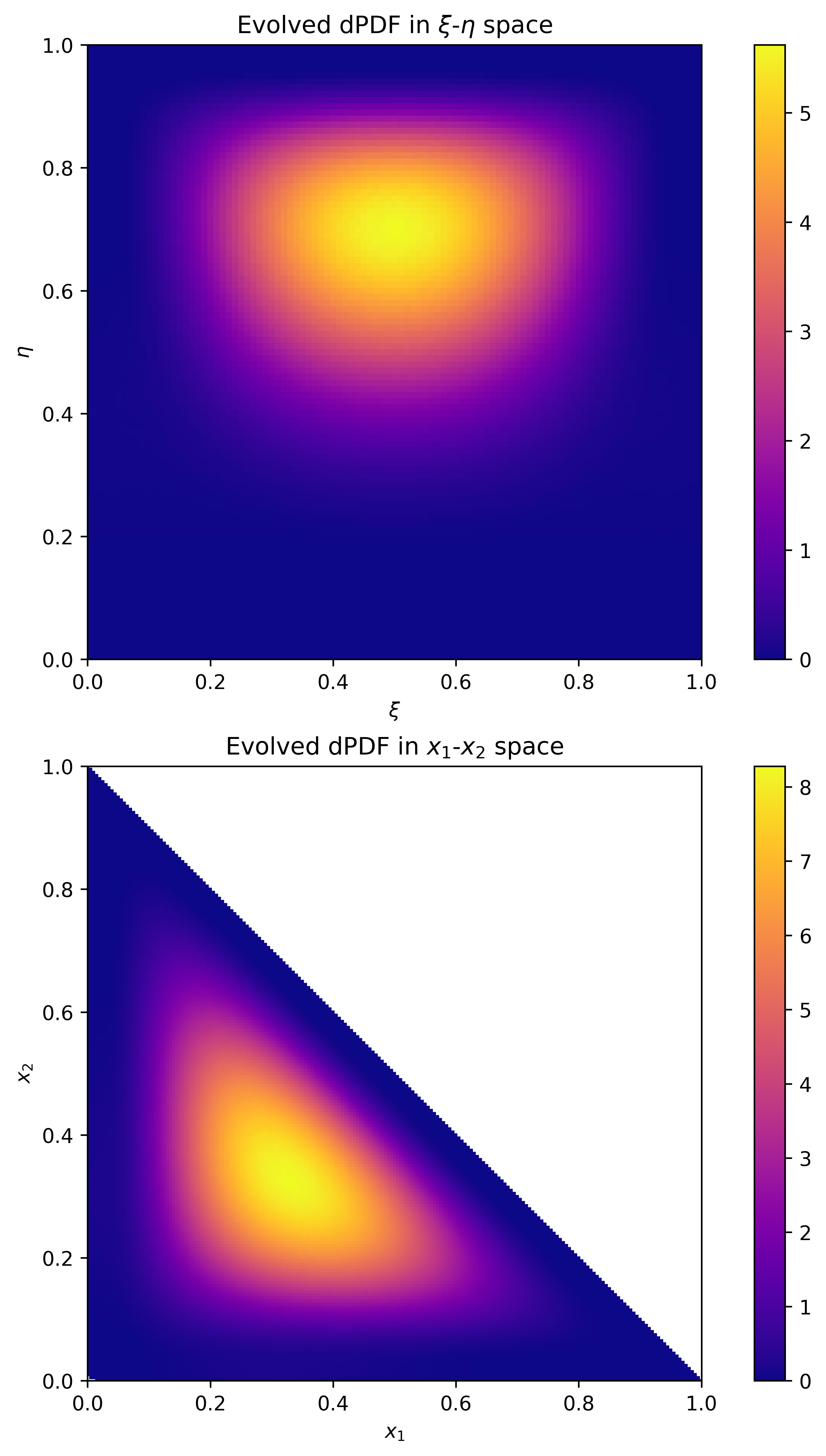
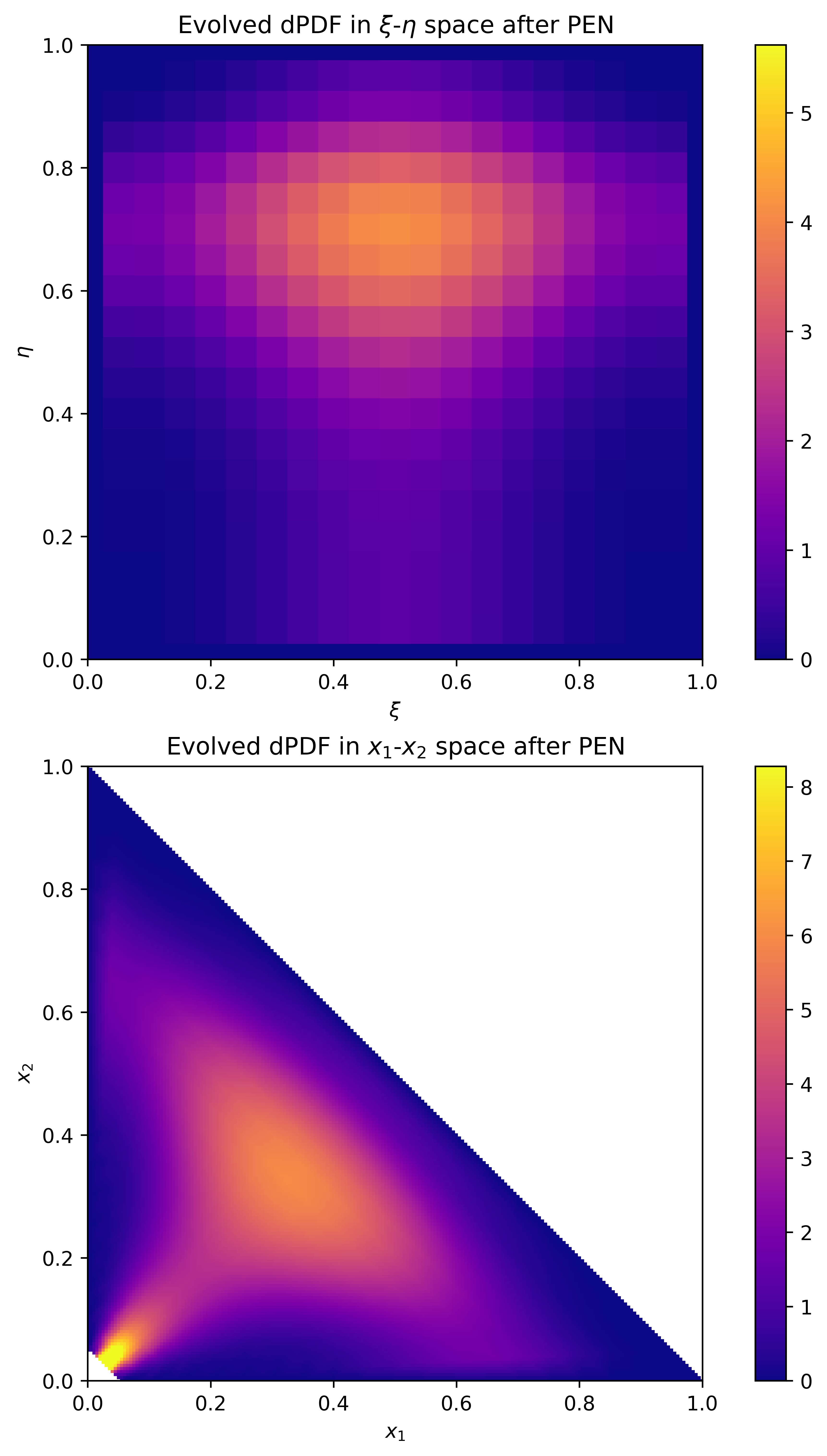
Figure 4: Contour plots of the dPDF at $Q^{2}/Q^{2}_{0}=100$ with $\alpha_{s}=0.1$, $x=0.1$, and $Q_{0}=m_{q}$ as a function of $\eta=x_{1}+x_{2}$ and $\xi=x_{1}/(x_{1}+x_{2})$ (top), and $x_{1}$ and $x_{2}$ (bottom). Left: the dPDF obtained here from the Brodsky-Schlumpf model LCwf with corrections due to collinear gluon emission. Right: same, after the removal of quantum correlations via the PEN transformation.

Our numerical results are shown in fig. 4. The maximum of the dPDF occurs at $\xi=1/2$, of course, and near $\eta=2/3$. The strength of this peak is reduced by the PEN transformation. On the other hand, it enhances the dPDF for asymmetric momentum fractions (small or large $\xi$) when either one of them is large ($\eta=2/3\pm 0.15$). PEN also enhances the dPDF for similar ($\xi=1/2\pm 0.15$) but fairly small ($\eta\lesssim 0.3$) momentum fractions. Put the other way: entanglement correlations associated with the negativity tend to suppress the dPDF for small (and similar) as well as for large but strongly asymmetric momentum fractions, but instead strengthen the peak near $x_{1}=x_{2}$ and $x_{1}+x_{2}=2/3$. Thus, after evolution to higher $Q^{2}$ the strongest effects from quantum correlations appear in a different regime than at the initial scale $Q_{0}^{2}$; we recall from sec. II.4 that for the non-perturbative constituent quark LCwf the strongest effects occurred for rather asymmetric momentum fractions $x_{1}$ and $x_{2}$, and well below the kinematic boundary $x_{1}+x_{2}=1$.

IV Summary

The density matrix $\rho_{x_{1}x_{2},x_{1}^{\prime}x_{2}^{\prime}}$ describing the LC momentum distributions of two quarks in the proton is obtained by tracing the pure proton state $\left|P\right\rangle\,\left\langle P\right|$ over all unobserved degrees of freedom. This, in general, results in a mixed state with non-zero von Neumann entropy. The purpose of this paper was to apply methods from Quantum Information Theory, specifically the negativity measure, to investigate quantum entanglement correlations of double quark momentum fractions.

The diagonal $f_{qq}(x_{1},x_{2})=\rho_{x_{1}x_{2},x_{1}x_{2}}$ of the density matrix corresponds to the double quark parton distribution (dPDF). In general the dPDF differs from the product of two single quark PDFs due to correlations. Classical correlations can be encoded in probabilistic mix of product states, i.e. a separable state (4); for such a state the “entanglement negativity” measure of Quantum Information Theory is zero. On the other hand, a non-zero negativity implies the presence of non-separable quantum correlations.

In sec. II we have computed the density matrix over the two-quark LC momentum fractions in an effective LC constituent quark model of the proton intended for not too small $x_{i}\sim 0.1$ or greater, and a low resolution scale $Q_{0}^{2}$. Upon purging the density matrix of its entanglement negativity and the associated quantum correlations, we observe strong modifications of the dPDF in some range of momentum fractions, specifically for asymmetric $x_{1},x_{2}$ far below the bound $x_{1}+x_{2}=1$. In fact, in this regime we find that purging the entanglement negativity turns a suppression of the quantum correlated dPDF (relative to a product of two single quark PDFs) into a strong enhancement. On the other hand, for large $x_{1}+x_{2}$ or $x_{1}\simeq x_{2}$ the effect of such quantum correlations in this model is found to be small whereas classical correlations enforce $f_{qq}(x_{1},x_{2})/f_{q}(x_{1})f_{q}(x_{2})\to 0$ as $x_{1}+x_{2}\to 1$.

In sec. III we derived the corrections to $\rho_{x_{1}x_{2},x_{1}^{\prime}x_{2}^{\prime}}$ due to the emission of one collinear gluon. This corresponds to one step of QCD scale evolution to $Q^{2}>Q_{0}^{2}$ of the entire density matrix, assuming $\alpha_{s}\log Q^{2}/Q_{0}^{2}\ll 1$; on the diagonal we recover the dPDF DGLAP evolution in terms of convolutions of splitting functions and dPDFs. From the density matrix at the new scale $Q^{2}$ we obtain first qualitative predictions for the QCD scale evolution of quantum entanglement in double quark states in the proton. Interestingly, at the higher scale we do observe significant effects due to quantum correlations for nearly symmetric momentum fractions, $x_{1}\simeq x_{2}$, for fairly small $x_{1}+x_{2}\lesssim 0.3$, where their effect is to suppress the dPDF. These initial explorations motivate the development of the complete QCD evolution equations of the full two-quark density matrix, to account for the emission of an entire ladder of partons. This work is in progress.

References

- Korotkikh and Snigirev [2004] V. L. Korotkikh and A. M. Snigirev, Double parton correlations versus factorized distributions, Phys. Lett. B 594, 171 (2004), arXiv:hep-ph/0404155 .
- Gaunt and Stirling [2010] J. R. Gaunt and W. J. Stirling, Double Parton Distributions Incorporating Perturbative QCD Evolution and Momentum and Quark Number Sum Rules, JHEP 03, 005, arXiv:0910.4347 [hep-ph] .
- Blok et al. [2011] B. Blok, Y. Dokshitzer, L. Frankfurt, and M. Strikman, The Four jet production at LHC and Tevatron in QCD, Phys. Rev. D 83, 071501 (2011), arXiv:1009.2714 [hep-ph] .
- Diehl et al. [2012] M. Diehl, D. Ostermeier, and A. Schafer, Elements of a theory for multiparton interactions in QCD, JHEP 03, 089, [Erratum: JHEP 03, 001 (2016)], arXiv:1111.0910 [hep-ph] .
- Diehl and Gaunt [2018] M. Diehl and J. R. Gaunt, Double parton scattering theory overview, Adv. Ser. Direct. High Energy Phys. 29, 7 (2018), arXiv:1710.04408 [hep-ph] .
- Jaarsma et al. [2023] M. Jaarsma, R. Rahn, and W. J. Waalewijn, Towards double parton distributions from first principles using Large Momentum Effective Theory, JHEP 12, 014, arXiv:2305.09716 [hep-ph] .
- Broniowski and Arriola [2014] W. Broniowski and E. R. Arriola, Valence double parton distributions of the nucleon in a simple model, Few-Body Syst 55, 381 (2014), arXiv:1310.8419 [hep-ph] .
- Golec-Biernat and Lewandowska [2014] K. Golec-Biernat and E. Lewandowska, How to impose initial conditions for QCD evolution of double parton distributions?, Phys. Rev. D 90, 014032 (2014), arXiv:1402.4079 [hep-ph] .
- Armesto et al. [2019] N. Armesto, F. Dominguez, A. Kovner, M. Lublinsky, and V. Skokov, The Color Glass Condensate density matrix: Lindblad evolution, entanglement entropy and Wigner functional, JHEP 05, 025, arXiv:1901.08080 [hep-ph] .
- Golec-Biernat et al. [2015] K. Golec-Biernat, E. Lewandowska, M. Serino, Z. Snyder, and A. M. Stasto, Constraining the double gluon distribution by the single gluon distribution, Phys. Lett. B 750, 559 (2015), arXiv:1507.08583 [hep-ph] .
- Chang et al. [2013] H.-M. Chang, A. V. Manohar, and W. J. Waalewijn, Double Parton Correlations in the Bag Model, Phys. Rev. D 87, 034009 (2013), arXiv:1211.3132 [hep-ph] .
- Rinaldi et al. [2014] M. Rinaldi, S. Scopetta, M. Traini, and V. Vento, Double parton correlations and constituent quark models: a Light Front approach to the valence sector, JHEP 12, 028, arXiv:1409.1500 [hep-ph] .
- Rinaldi and Ceccopieri [2017] M. Rinaldi and F. A. Ceccopieri, Relativistic effects in model calculations of double parton distribution function, Phys. Rev. D 95, 034040 (2017), arXiv:1611.04793 [hep-ph] .
- Rinaldi et al. [2016] M. Rinaldi, S. Scopetta, M. C. Traini, and V. Vento, Correlations in Double Parton Distributions: Perturbative and Non-Perturbative effects, JHEP 10, 063, arXiv:1608.02521 [hep-ph] .
- Reitinger et al. [2024] D. Reitinger, C. Zimmermann, M. Diehl, and A. Schäfer, Double parton distributions with flavor interference from lattice QCD, JHEP 04, 087, arXiv:2401.14855 [hep-lat] .
- Kharzeev and Levin [2017] D. E. Kharzeev and E. M. Levin, Deep inelastic scattering as a probe of entanglement, Phys. Rev. D 95, 114008 (2017), arXiv:1702.03489 [hep-ph] .
- Kharzeev [2021] D. E. Kharzeev, Quantum information approach to high energy interactions, Phil. Trans. A. Math. Phys. Eng. Sci. 380, 20210063 (2021), arXiv:2108.08792 [hep-ph] .
- Kharzeev and Levin [2021] D. E. Kharzeev and E. Levin, Deep inelastic scattering as a probe of entanglement: Confronting experimental data, Phys. Rev. D 104, L031503 (2021), arXiv:2102.09773 [hep-ph] .
- Kovner and Lublinsky [2015] A. Kovner and M. Lublinsky, Entanglement entropy and entropy production in the Color Glass Condensate framework, Phys. Rev. D 92, 034016 (2015), arXiv:1506.05394 [hep-ph] .
- Kovner et al. [2019] A. Kovner, M. Lublinsky, and M. Serino, Entanglement entropy, entropy production and time evolution in high energy QCD, Phys. Lett. B 792, 4 (2019), arXiv:1806.01089 [hep-ph] .
- Duan et al. [2022] H. Duan, A. Kovner, and V. V. Skokov, Gluon quasiparticles and the CGC density matrix, Phys. Rev. D 105, 056009 (2022), arXiv:2111.06475 [hep-ph] .
- Dumitru et al. [2023] A. Dumitru, A. Kovner, and V. V. Skokov, Entanglement entropy of the proton in coordinate space, Phys. Rev. D 108, 014014 (2023), arXiv:2304.08564 [hep-ph] .
- Hentschinski et al. [2024] M. Hentschinski, D. E. Kharzeev, K. Kutak, and Z. Tu, QCD evolution of entanglement entropy, Rept. Prog. Phys. 87, 120501 (2024), arXiv:2408.01259 [hep-ph] .
- Hatta and Montgomery [2024] Y. Hatta and J. Montgomery, Maximally entangled gluons for any , (2024), arXiv:2410.16082 [hep-ph] .
- Bhattacharya et al. [2024] S. Bhattacharya, R. Boussarie, and Y. Hatta, Spin-orbit entanglement in the Color Glass Condensate, Phys. Lett. B 859, 139134 (2024), arXiv:2404.04208 [hep-ph] .
- Gurvits [2003] L. Gurvits, Classical deterministic complexity of Edmonds’ Problem and quantum entanglement, in 35th annual ACM symposium on Theory of computing (2003).
- Gharibian [2010] S. Gharibian, Strong NP-hardness of the quantum separability problem, Quant. Inf. Comput. 10, 0343 (2010), arXiv:0810.4507 [quant-ph] .
- Gühne and Tóth [2009] O. Gühne and G. Tóth, Entanglement detection, Phys. Rept. 474, 1 (2009), arXiv:0811.2803 [quant-ph] .
- Horodecki et al. [2009] R. Horodecki, P. Horodecki, M. Horodecki, and K. Horodecki, Quantum entanglement, Rev. Mod. Phys. 81, 865 (2009), arXiv:quant-ph/0702225 .
- Chruscinski and Sarbicki [2014] D. Chruscinski and G. Sarbicki, Entanglement witnesses: construction, analysis and classification, J. Phys. A 47, 483001 (2014), arXiv:1402.2413 [quant-ph] .
- Donald et al. [2002] M. J. Donald, M. Horodecki, and O. Rudolph, The uniqueness theorem for entanglement measures, Journal of Mathematical Physics 43, 4252–4272 (2002).
- Peres [1996] A. Peres, Separability Criterion for Density Matrices, Phys. Rev. Lett. 77, 1413 (1996), arXiv:quant-ph/9604005 [quant-ph] .
- Horodecki et al. [1996] M. Horodecki, P. Horodecki, and R. Horodecki, Separability of mixed states: necessary and sufficient conditions, Phys. Lett. A 233, 1 (1996), arXiv:quant-ph/9605038 [quant-ph] .
- Wilde [2011] M. M. Wilde, From Classical to Quantum Shannon Theory 10.1017/9781316809976.001 (2011), arXiv:1106.1445 [quant-ph] .
- Schlumpf [1993] F. Schlumpf, Relativistic constituent quark model of electroweak properties of baryons, Phys. Rev. D 47, 4114 (1993), [Erratum: Phys.Rev.D 49, 6246 (1994)], arXiv:hep-ph/9212250 .
- Brodsky and Schlumpf [1994] S. J. Brodsky and F. Schlumpf, Wave function independent relations between the nucleon axial coupling and the nucleon magnetic moments, Phys. Lett. B 329, 111 (1994), arXiv:hep-ph/9402214 .
- Bakker et al. [1979] B. L. G. Bakker, L. A. Kondratyuk, and M. V. Terentev, On the formulation of two-body and three-body relativistic equations employing light front dynamics, Nucl. Phys. B 158, 497 (1979).
- Qian et al. [2024] C. Qian, S. Xu, Y.-G. Yang, and X. Zhao, Quark and gluon entanglement in the proton based on a light-front Hamiltonian, (2024), arXiv:2412.11860 [hep-ph] .
- Dumitru and Kolbusz [2023] A. Dumitru and E. Kolbusz, Quark pair angular correlations in the proton: Entropy versus entanglement negativity, Phys. Rev. D 108, 034011 (2023), arXiv:2303.07408 [hep-ph] .
- Dahl et al. [2007] G. Dahl, J. Leinaas, J. Myrheim, and E. Ovrum, A tensor product matrix approximation problem in quantum physics, Linear Algebra and its Applications 420, 711 (2007).
- Dumitru and Kolbusz [2022] A. Dumitru and E. Kolbusz, Quark and gluon entanglement in the proton on the light cone at intermediate , Phys. Rev. D 105, 074030 (2022), arXiv:2202.01803 [hep-ph] .
- Dumitru and Paatelainen [2021] A. Dumitru and R. Paatelainen, Sub-femtometer scale color charge fluctuations in a proton made of three quarks and a gluon, Phys. Rev. D 103, 034026 (2021), arXiv:2010.11245 [hep-ph] .
- Lepage [2021] G. P. Lepage, Adaptive multidimensional integration: VEGAS enhanced, J. Comput. Phys. 439, 110386 (2021), arXiv:2009.05112 [physics.comp-ph] .
- Lepage [2013] G. P. Lepage, vegas 6.2 – project description, https://pypi.org/project/vegas/ (2013).