A Hybrid Supervised and Self-Supervised Graph Neural Network for Edge-Centric Applications

Abstract

This paper presents a novel graph-based deep learning model for tasks involving relations between two nodes (edge-centric tasks), where the focus lies on predicting relationships and interactions between pairs of nodes rather than node properties themselves. This model combines supervised and self-supervised learning, taking into account for the loss function the embeddings learned and patterns with and without ground truth. Additionally it incorporates an attention mechanism that leverages both node and edge features. The architecture, trained end-to-end, comprises two primary components: embedding generation and prediction. First, a graph neural network (GNN) transform raw node features into dense, low-dimensional embeddings, incorporating edge attributes. Then, a feedforward neural model processes the node embeddings to produce the final output. Experiments demonstrate that our model matches or exceeds existing methods for protein-protein interactions prediction and Gene Ontology (GO) terms prediction. The model also performs effectively with one-hot encoding for node features, providing a solution for the previously unsolved problem of predicting similarity between compounds with unknown structures.

I Introduction

Graphs are versatile structures used to model relationships between entities, particularly in scenarios where data does not have an Euclidean structure. Each node in a graph represents an entity, and edges describe relationships between pairs of nodes. Furthermore, nodes and edges can have features that describe properties associated with them. This flexibility makes graphs useful in various applications, including social networks [1], recommendation systems[2, 3], and bioinformatics, where they are employed to model intricate biological interactions [4].

Early approaches to graph analysis focused on using metrics such as connectivity, centrality, and other structural properties to describe graph features [5]. While useful for analyzing static properties, these methods do not learn from the graph in a way that captures complex relationships or patterns within the data. One of the earliest methods for generating node embeddings from graphs is DeepWalk [6]. This approach uses random walks to explore each node’s local neighborhood and then applies a skip-gram model to convert these walks into dense embeddings. However, it does not leverage edge weighting, which can limit its applicability. LINE [7] follows, focusing on preserving both first- and second-order proximity in the embeddings but also does not consider edge features. Node2Vec [8] extends the random walk approach by adjusting the exploration strategy for more flexible neighborhood sampling; however, it relies on fixed, non-learnable edge weights, which limits its adaptability. Despite their successes, these approaches have critical limitations: they do not share parameters across nodes, leading to inefficiencies as graphs grow, and they struggle to generalize to dynamic or unseen graphs [9]. These shortcomings underscore the need for more advanced methods capable of capturing both node and edge information in a flexible, scalable manner, setting the stage for more powerful models.

Graph Neural Networks (GNNs) have emerged as a powerful approach for addressing the limitations of traditional methods by learning from the structure of graph neighborhoods [10]. These models aim to generate new representations for entities based on their connections within the graph, leveraging the inherent relationships between nodes and edges. There are two primary approaches for constructing GNNs: spectral and spatial methods, each with its own advantages, drawbacks, and applications.

Spectral methods define graph convolutions using spectral graph theory, where the graph is transformed into the spectral domain, typically employing the graph Fourier transform [11, 12]. By leveraging the spectral components of the Laplacian matrix, these methods capture global patterns in the graph. However, they can be computationally expensive, especially for large-scale graphs, due to the need for eigenvalue decomposition of the Laplacian matrix [13, 14]. Furthermore, spectral-based models often struggle to generalize to graphs with different structures, limiting their applicability in inductive learning tasks [15, 16]. To address these issues, the GCN/ChebNet method was proposed, which uses polynomial approximations of spectral filters to reduce computational overhead [12]. However, these methods require the graph to remain unchanged during the learning process, limiting their flexibility in dynamic graph scenarios.

Spatial approaches define convolutions directly on the graph by aggregating information from neighboring nodes [10]. These methods propagate information locally, with each node passing messages to its neighbors, refining node representations iteratively [15]. Spatial methods in graph learning offer key advantages over spectral approaches, particularly in computational efficiency and flexibility. Unlike spectral methods, which require costly eigenvalue decomposition of the graph Laplacian, spatial methods operate directly on the graph structure, making them more scalable for large graphs with millions of nodes and adaptable to dynamic graphs without recalculating eigenvalues. They also generalize better to unseen nodes or graphs during training, a process known as inductive learning. This is particullarly important in scenarios where new data is constantly encountered [17]. Spatial methods also allow edge features into the learning process, which can provide relevant information for modeling complex relationships between nodes.

One of the most recent approaches in this field is the Message Passing Neural Network (MPNN) [18], which has proven effective across tasks ranging from protein-protein interaction prediction to gene regulatory network analysis [19, 20]. MPNNs are a class of GNN designed to handle graph-based tasks by iteratively passing messages between nodes and updating node representations based on the messages sent by their local neighborhood. The core idea is to aggregate information from a node’s neighbors and use this information to update the node’s feature representation. This process is particularly powerful for capturing the structural dependencies within graphs, making MPNNs highly versatile.

Formally, MPNNs operate through three main phases: message passing, node updating, and readout. At step $t$, the features $\mathbf{x}_{p}^{(t)}$ of node $p$ are updated by aggregating messages from its neighboring nodes according to:

$$m_{p}^{(t+1)}=\sum_{q\in\mathcal{N}(p)}M_{t}\left(\mathbf{x}_{p}^{(t)},\mathbf{x}_{q}^{(t)},e_{pq}\right)$$ (1)

where $\mathcal{N}(p)$ denotes the set of neighbors of node $p$, and $M_{t}$ is the message function that depends on both node features and edge features $e_{pq}$. The features of the central node $p$ are then updated using information from its neighboring nodes:

$$\mathbf{x}_{p}^{(t+1)}=U_{t}\left(\mathbf{x}_{p}^{(t)},m_{p}^{(t+1)}\right)$$ (2)

where $U_{t}$ is the node update function, which typically combines the features of neighboring nodes with aggregated messages, using schemes such as sum, mean, or maximum to update each node’s representation. After several iterations of message passing, the final node states can be aggregated using a readout function:

$$\hat{y}=R\left(\{\mathbf{x}_{p}^{(K)}|p\in\mathcal{G}\}\right)$$ (3)

The readout function $R$ in Eq 3 aggregates information from all nodes to produce a graph-level or sub-graph-level representation $\hat{y}$, which can be used for classification or regression tasks involving graph, nodes or edges. This architecture has proven highly effective in many applications, yet it has limitations in handling edge-centric tasks, which involve learning relationships between pairs of nodes rather than individual nodes.

Despite the success of MPNNs in node-level tasks, significant challenges remain when it comes to generalizing to large-scale or highly complex graphs and addressing edge-centric tasks such as regression and classification on graph edges. Many traditional GNN models, including MPNNs, focus primarily on node-level features while underutilizing the information contained in edge attributes, which is particularly relevant in fields like bioinformatics, where interactions between entities often occur at the edge level [4].

Based on the strengths of MPNNs, in this work we proposes a new MPNN-based model trained with a custom loss function designed to handle both supervised and self-supervised learning. Our model incorporates both node and edge features into the prediction process, making it capable of handling complex relationships between entities in graphs. Furthermore, we employ an attention mechanism inspired by transformers [21], which enhances the model’s ability to capture intricate dependencies within the graph. This architecture also proves robust even when simple one-hot encodings are used for node features, allowing the model to perform effectively even in cases where node information is sparse or missing.

II Materials and methods

This work presents a neural model composed of two main parts: an embedding block and a prediction block. The prediction block produces an estimation for pairs of nodes in the graph. This section presents the theoretical concepts and materials used in this work. First, we describe the embedding block. Then, we show the prediction block and its components, and explain the process of building the dataset.

II-A Graph and subgraph definitions

Let $\mathcal{G}=\{v,e\}$ be a graph, where $v$ is the set of $|v|$ nodes in the network, and $e$ denotes the set of edges connecting the theme. Let $\mathbf{X}\in\mathbb{R}^{|v|\times d}$ be the feature matrix of nodes in $\mathcal{G}$, where $d$ is the number of features for each node. Furthermore, let $\mathcal{E}\in\mathbb{R}^{|e|\times q}$ denote the edge feature matrix, where each row represents the features associated with a specific edge in the graph. These edge features may or may not exist and can be a vector of arbitrary size $q$. Figure 1a shows an example of a typical graph and its elements.

The subgraph $\mathcal{G}^{\prime}_{i,j}=\{v_{i,j},e_{i,j}\}\subseteq\mathcal{G}$ is defined as being induced by nodes $i$ and $j$ (Figure 1b), where $v_{i,j}=\{\mathcal{N}(i),\mathcal{N}(j)\}$ are the nodes included, and $e_{i,j}$ are the connections between them. The set $\mathcal{N}(k)$ is represented by the direct neighbors that share an edge with node $k$. Additionally, the edge features matrix $\mathbf{E}^{\prime}_{\mathcal{G}^{\prime}_{i,j}}\in\mathbb{R}^{|e_{i,j}|\times q}$ is associated with $|e_{i,j}|$ number of connections in the subgraph $\mathcal{G}^{\prime}_{i,j}$. The feature matrix $\mathbf{X}^{\prime}_{\mathcal{G}^{\prime}_{i,j}}\in\mathbb{R}^{|v_{i,j}|\times d}$ is also defined for the $|v_{i,j}|$ nodes in the subgraph $\mathcal{G}^{\prime}_{i,j}$.

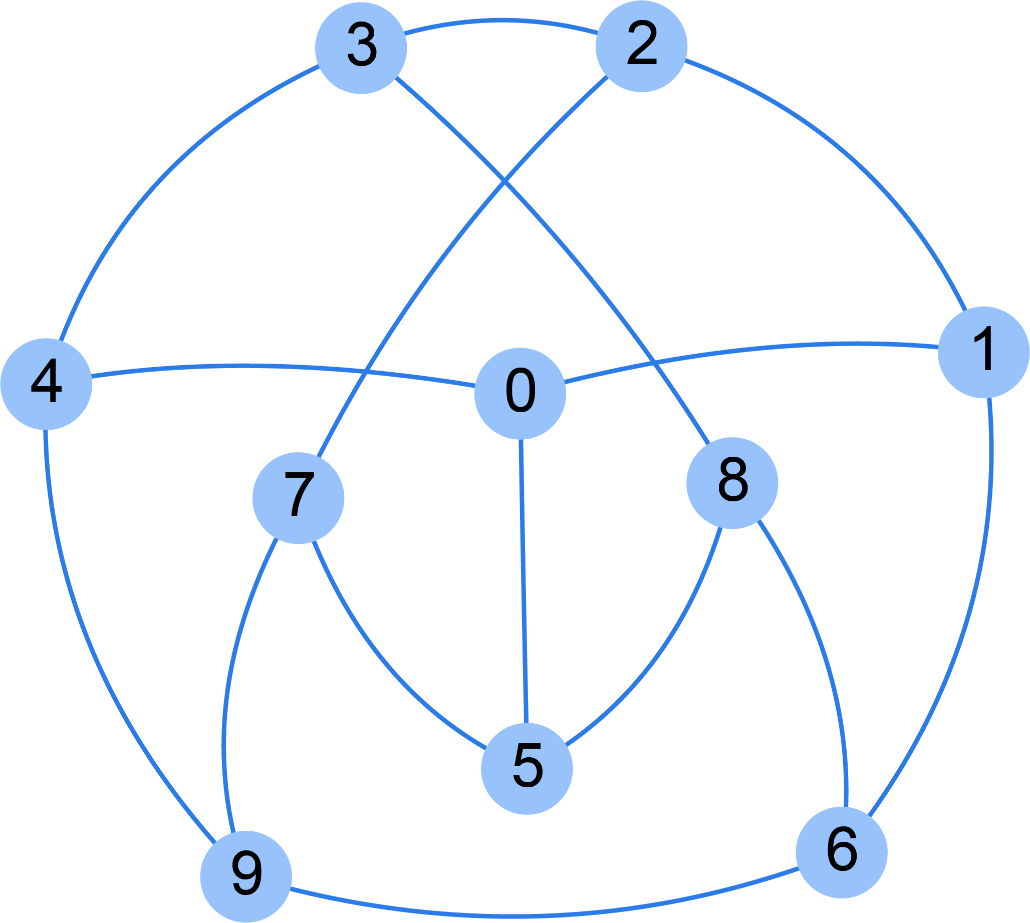
((a))

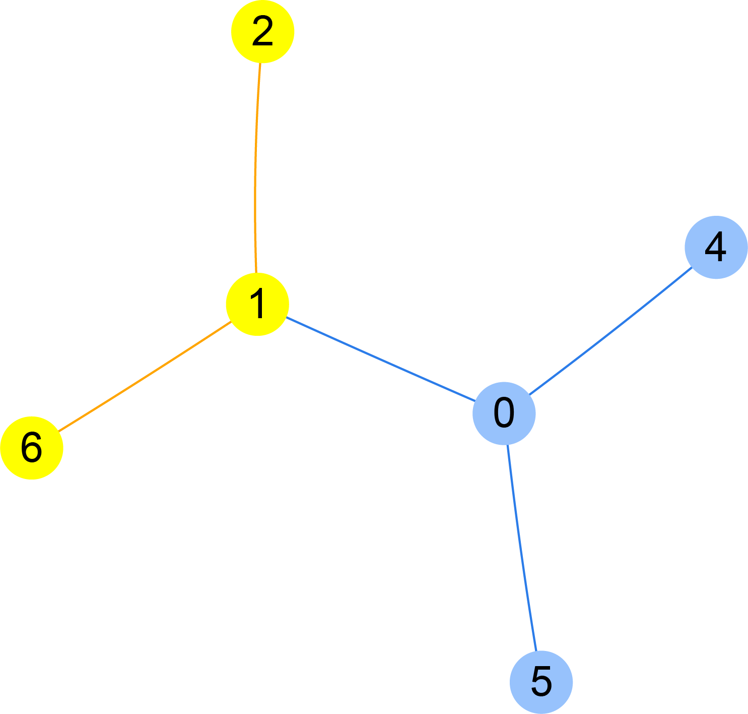
((b))

Figure 1: (a) Example of a graph $\mathcal{G}$. (b) Example of pattern subgraph $\mathcal{G}^{\prime}_{0,1}$ induced for nodes 0 and 1. Nodes and edges related to node 1 are highlighted in yellow, while those related to node 0 are shown in blue. These represent the first-degree neighbors of each node within the subgraph. These graphs represent only the structure; in this representation, each node is associated with a feature vector, and each edge has corresponding edge features.

II-B Proposed model

Our model operates on subgraphs $\mathcal{G}^{\prime}$, structured around two central nodes. This approach is essential for edge-centric tasks, where the aim is to predict the presence or properties of connections between specific pairs of nodes. The subgraph is constructed to enrich the representation of these central nodes by leveraging their local neighborhood. In each subgraph, the central nodes and their direct neighbors, along with all existing edges among these nodes, form the context for learning.

The model processes each subgraph in two stages: embedding generation and prediction. In the embedding generation phase, the node features within the subgraph are transformed into dense, low-dimensional vectors $\mathbf{Z}$ that capture both structural and feature-based information. These embeddings, particularly those of the central nodes, are then concatenated and passed to the prediction module to estimate the desired property associated with their connection. The entire model is trained end-to-end using a loss function that combines supervised and self-supervised training, allowing it to learn meaningful patterns even for nodes with limited or missing initial information. Figure 2 illustrates the model’s architecture, with detailed descriptions of each component provided in the following sections.

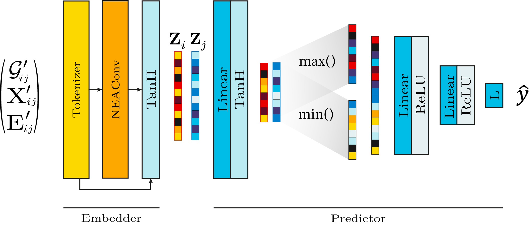
Figure 2: Model architecture overview. The input consists of the pattern subgraph $\mathcal{G}^{\prime}_{i,j}$, node features $\mathbf{X}^{\prime}_{\mathcal{G}^{\prime}_{i,j}}$, and edge features $\mathbf{E}^{\prime}_{\mathcal{G}^{\prime}_{i,j}}$. These inputs are processed through the embedding generation block: Tokenizer, the NodeEdgeAttentionConv (NEAConv) layer, and Tanh to form the embeddings $Z_{i}$ and $Z_{j}$. The embeddings then pass through a linear layer followed by a Tanh activation, are reordered, and finally fed into a three-layer perceptron to produce the output.

II-C Embedding generation

This block involves two components: the tokenizer and the NodeEdgeAttentionConv (NEAConv) layer, as illustrated in Figure 2. Node embeddings are compact, low-dimensional representations of graph nodes, integrating both node and edge features. Our model effectively generates these embeddings, capturing the underlying graph structure and node characteristics even when one-hot encoding is used as node features. This capability ensures efficient information propagation and accurate downstream predictions. We focus on the architecture and mechanisms used in our model to produce these meaningful representations that encode the underlying graph structure, node characteristics, and edge information.

The tokenizer takes the node features $\mathbf{X}^{\prime}_{\mathcal{G}^{\prime}_{i,j}}$ as input and projects them into a more suitable space for inference using a Multi-Layer Perceptron (MLP), yielding a new representation $\widetilde{\mathbf{X}}^{\prime}_{\mathcal{G}^{\prime}_{i,j}}$. This representation is then processed by the NEAConv layer, a message-passing neural network specifically designed for edge-centric tasks. In this layer, custom message and update functions are defined to align with our model architecture.

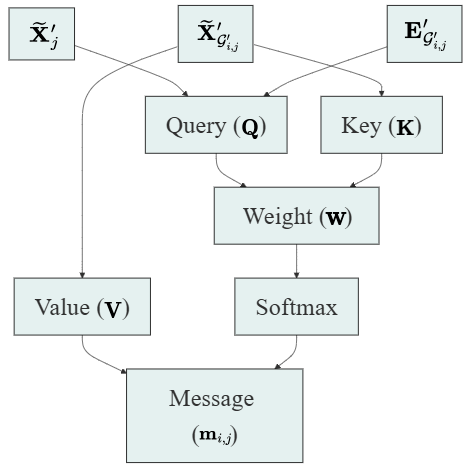
Figure 3: Diagram illustrating the attention mechanism in the message function. It shows how node and edge features are transformed into key, query, and value vectors to assign attention weights, facilitating effective information aggregation from neighboring nodes.

Figure 3, shows the message-passing process involved in the NEAConv layer. The information of each target node $i,j\in\mathcal{G}^{\prime}_{i,j}$ is updated through the attention mechanism described in Figure 3. For a given node $j$, the algorithm initially projects the tokenized features of the node $\widetilde{\mathbf{X}}^{\prime}_{j}$ and those of all the pattern $\widetilde{\mathbf{X}}^{\prime}_{\mathcal{G}^{\prime}_{i,j}}$ into three new spaces with the same dimension as the original.

These nonlinear projections are performed by three separate perceptrons, each consisting of a linear layer followed by a sigmoid activation: The query vector $\mathbf{Q}$ is generated from the concatenation of the target node features $\widetilde{\mathbf{X}}^{\prime}_{j}$ and, when available, the edge features $\mathbf{E}^{\prime}_{\mathcal{G}^{\prime}_{i,j}}$, capturing the relevance of the target node within the context of its surrounding neighborhood. The key vector $\mathbf{K}$ is derived from the source nodes’ features $\widetilde{\mathbf{X}}^{\prime}_{\mathcal{G}^{\prime}_{i,j}}$, encoding essential information about the source nodes to be compared with the query vector. The value vector $\mathbf{V}$, also generated from the source nodes’ features $\widetilde{\mathbf{X}}^{\prime}_{\mathcal{G}^{\prime}_{i,j}}$, carries the information that will be propagated to the target node. The vector weight $\mathbf{w}$ which represents the importance of each source node’s information for the target node, is calculated as:

$$\mathbf{w}=\text{sum}(\mathbf{Q}\odot\mathbf{K},\text{dim}=1)$$ (4)

where $\mathbf{Q}\odot\mathbf{K}$ represents the element-wise (Hadamard) product of the two tensors. This vector $\mathbf{w}$ is then normalized using a softmax function. The normalized vector $\mathbf{w}$ is then used to construct the new representation $\widehat{\mathbf{X}}^{\prime}_{j}$ of the central node, through the weighted combination of the representations $\mathbf{V}$ of the neighboring nodes. The update function concatenates the aggregated messages:

$$\widehat{\mathbf{X}}^{\prime}_{j}=\sum_{k\in\mathcal{N}(j)}\ \mathbf{m}_{k,j}$$ (5)

with the original tokenized node features $\widetilde{\mathbf{X}}^{\prime}_{j}$ resulting in updated embeddings that integrate both the aggregated information and the original features:

$${\mathbf{Z}_{j}=Tanh\left(\left[\widehat{\mathbf{X}}^{\prime}_{j},\widetilde{\mathbf{X}}^{\prime}_{j}\right]\right)}$$ (6)

II-D Prediction step

The prediction module in our model is a multilayer perceptron (MLP) designed to process the generated node embeddings and produce task-specific predictions. To ensure that the model’s predictions are invariant to the permutation of the nodes, we first perform a reordering of the features from the node embeddings. This reordering helps in capturing the important features across different nodes while maintaining the permutation invariance property. Initially, we extract the minimum and maximum values along the feature dimension of the node embeddings. These extracted features are then concatenated to form a new feature representation that encapsulates the critical information from the node embeddings. The architecture of the MLP consists of three linear layers, each followed by an activation function, to produce the final prediction output.

II-E Loss function

The proposed loss function is build for optimizing node embeddings and predictions simultaneously. This is defined as:

$$\mathcal{L}=\alpha\mathcal{L}_{\text{supervised}}+\beta\mathcal{L}_{\text{cosine}}+\gamma\mathcal{L}_{\text{cosine\_pred}}$$ (7)

where $\alpha$, $\beta$, and $\gamma$ are weighting coefficients.

$\mathcal{L}_{\text{supervised}}$ and $\mathcal{L}_{\text{cosine}}$ are supervised terms that guide the model to align its predictions and embeddings with the true labels, while $\mathcal{L}_{\text{cosine\_pred}}$ serves as a self-supervised term, refining the embeddings by aligning the predictions with the cosine similarity of the node embeddings. All three terms follow the same structure: for regression tasks, the Mean Squared Error (MSE) is used, and for classification tasks, the cross-entropy loss is applied.

The term $\mathcal{L}_{\text{supervised}}$ minimizes the difference between the predicted outputs $\hat{Y}$ and the true labels $Y$, ensuring accurate predictions. Similarly, $\mathcal{L}_{\text{cosine}}$ compares the cosine similarity of the node embeddings, denoted as $\widetilde{Y}$ (see equation 8), to the ground truth $Y$, guiding the model to learn embeddings that reflect meaningful relationships between nodes. Both terms apply MSE for regression and cross-entropy for classification, depending on the task.

$$\widetilde{Y}=cosine\_similarity(\mathbf{Z}_{i},\mathbf{Z}_{j})$$ (8)

In addition to the supervised terms, the loss function includes a self-supervised component, $\mathcal{L}_{\text{cosine\_pred}}$, which aligns the predicted output $\hat{Y}$ with the cosine similarity of the node embeddings $\widetilde{Y}$. This self-supervised term helps the model learn robust representations even for nodes with unknown or incomplete information by structuring the embeddings in a meaningful way. As a result, the model becomes more adaptable to scenarios where data is missing, improving its generalization and performance. During training, if an input pattern does not hace true labels assigned, only the third term will be used, allowing the model to learn in a unsupervized way.

The combination of these terms allows the model to learn more robust and generalizable embeddings, as well as make accurate predictions. The inclusion of nodes with unknown information in the loss function ensures that the embeddings capture the overall structure and relationships within the graph, improving the representation of all nodes, regardless of the availability of explicit labels.

III Datasets

Experimental evaluation of the proposed model was performed using three bioinformatic tasks: protein-protein interaction prediction, Gene Ontology (GO) annotation prediction, and metabolic compounds structural similarity prediction. The first task entails identifying potential interactions between proteins by analyzing structural, sequence, and functional data. The second task involves assigning an annotation of molecular functions, biological processes, or cellular components to genes or proteins based on the annotations of the known genes and all genes expression data. Finally, the last task consists of predicting the similarity between metabolic compounds that participate in the same metabolic network based on the structure of the neighborhood they share, without considering their molecular structure.

III-A Protein-Protein Interaction

Five datasets used by Yang et al. [22] were taken into account for this task. HPRD dataset involves  36k pairs of known protein interactions (positive patterns), and  36k pairs of artificial interactions constructed by randomly pairing proteins from different subcellular locations (negative patterns). Human dataset includes  9k proteins, and  72k interactions; E. coli dataset comprises  2k proteins and 13k interactions; Drosophila dataset involves  7k proteins and  44k interactions; C. elegans dataset consists of  2,5k proteins, with  8k interactions. In all cases, datasets are balanced including equal number of positive and negative interactions.

The graph for each dataset was constructed by first calculating the similarity matrix between proteins using ClustalO [23]. This similarity matrix was then used by the k-Nearest Neighbors Graph (KNNG) algorithm [24] to create an undirected graph, with the number of neighbors $k$ determined experimentally. Various $k$ values were tested, keeping the model configuration fixed, to identify the optimal $k$ for capturing meaningful connections in the graph. Node features were build from sequence representations generated by the The Composition of Triads (CT) method, proposed by Shen et al. [25], represents protein sequences by projecting them into a vector space that counts the frequency of triad types. Initially, amino acids are grouped into seven categories based on dipole and side chain volume. Each amino acid in the sequence is then replaced by its category label, transforming the protein sequence into a sequence of integers. A sliding window of size three moves along this sequence to count occurrences of each triad type, treating every three consecutive amino acids as a unit. With seven categories, this yields 343 unique triad combinations. Similarity matrix between proteins were used as edge features.

III-B Gene Ontology (GO) terms

For this task, the objective is to predict new annotations for genes with unknow labels in the GO. The model was evaluated on three organisms: Saccharomyces cerevisiae, Arabidopsis thaliana, and Dictyostelium discoideum. These organisms were selected due to their extensive functional annotations, ensuring precise performance evaluation. The datasets used in this work are described in [26].

Gene expression data for the YEAST dataset, involving Saccharomyces cerevisiae, was sourced from [27]. From an initial 2,467 genes, 605 with 79 microarray values were selected after excluding those with missing data. GO annotations were applied following CAFA challenge guidelines [28]. After filtering out terms annotated to fewer than three genes, 422 genes remained for Biological Process (BP), 386 for Molecular Function (MF), and 442 for Cellular Component (CC). The ARA dataset, involving circadian-regulated genes in Arabidopsis thaliana under cold stress, comprised 1,546 genes, with 656 retaining BP annotations after filtering. Ultimately, 521 genes remained for BP, 315 for MF, and 740 for CC [29]. Gene expression data from Dictyostelium discoideum over a 24-hour development cycle constituted the DICTY dataset [30]. Initially, 707 genes with BP annotations were selected, and after filtering, 652 genes remained for BP, 366 for MF, and 630 for CC.

The expression vectors of each gene were used as node features, representing the gene’s expression profile, while the semantic similarity between each gene pair was used as edge features and to construct the $\mathcal{G}$ graph using the KNNG, which was then transformed into an undirected graph. Various $k$ values were tested, keeping the model configuration fixed, to identify the optimal $k$. The model is used to predict the semantic similarity for all unknown genes.

III-C Metabolic pathways

For this study, the objective is to predict the similarity of compounds included in metabolic pathways. We expanded upon our previous work [31] on the glycolysis metabolic pathway to include five additional metabolic pathways. Now encompasses the following pathways: Glycolysis, Starch and sucrose metabolism, Pentose phosphate pathway, Citrate cycle (TCA cycle), Pyruvate metabolism and Propanoate metabolism.

This expanded dataset comprises a total of 207 compounds, of which 174 have known structures and 33 have unknown structures. The dataset was constructed following the methodology in our previous work [31, 32]. Data were extracted from the KEGG (v95.2) database. For compounds with known structures, molecular structures were downloaded in SMILES format from the PubChem database. The RDKit library was used to calculate MACC keys [33] fingerprints for all compounds with known structures, as demonstrated in our previous work [32], where we showed the effectiveness of these fingerprints for this task. The Tanimoto coefficient [34] was then applied to calculate the similarity between compounds, as defined by:

$$T(\mathbf{c}_{i},\mathbf{c}_{j})=\frac{\sum_{k}(\mathbf{c}_{i}^{k}\wedge\mathbf{c}_{j}^{k})}{\sum_{k}(\mathbf{c}_{i}^{k}\vee\mathbf{c}_{j}^{k})}$$ (9)

where $\wedge$ and $\vee$ are the binary operators $and$ and $or$, respectively, and $\mathbf{c}_{i}$ and $\mathbf{c}_{j}$ are binary representations of the structures of compounds $i$ and $j$. The Tanimoto coefficient takes values in the range $[0,1]$ and calculates the proportion of shared features between the two structures. In total, 21,528 patterns were defined, resulting from the pairwise combinatorics of the 174 compounds with known structures and their interactions with compounds of unknown structure. Of these patterns, 5,390 are related to compounds with unknown structures.

For this dataset, one-hot vectors were used as node features to represent the compounds, while a one-hot vector based on the enzyme family that mediates the reaction served as edge features. These enzyme families are determined by the first digit of their KEGG EC number, ranging from 1 to 7 (e.g., 1 for Oxidoreductases, 2 for Transferases, and so forth). The EC numbers, standardized by the IUBMB/IUPAC, classify enzymes based on their biochemical reactions and are used in KEGG as ortholog identifiers (KOs) to link reactions with protein sequence data. In cases where multiple enzymes were involved, their one-hot vectors were aggregated. The construction of the metabolic pathway graph involved representing each compound as a node and connecting two nodes with an edge if they participated in a reaction as substrate and product. A comprehensive graph was built by integrating all reactions from the six specified metabolic pathways.

IV Results

The performance measure for protein-protein interaction (PPI) prediction was evaluated using the F1-score, which is derived from precision and recall. Precision is defined as the ratio of true positive predictions to the total predicted positives, expressed mathematically as:

$$\text{Precision}=\frac{TP}{TP+FP}$$ (10)

where $TP$ represents the number of true positives and $FP$ represents the number of false positives.

Recall, also known as sensitivity, is defined as the ratio of true positive predictions to the total actual positives, given by the equation:

$$\text{Recall}=\frac{TP}{TP+FN}$$ (11)

where $FN$ denotes the number of false negatives.

The F1-score is the harmonic mean of precision and recall, providing a single metric that balances both measures. It is calculated using the following equation:

$$F1=2\times\frac{\text{Precision}\times\text{Recall}}{\text{Precision}+\text{Recall}}$$ (12)

This score is particularly useful in the context of PPI prediction, as it takes into account both the accuracy of positive predictions and the ability to identify all relevant interactions.

For GO terms prediction results are reported according to the CAFA rules, with the maximum F1-measure ($\text{F}1_{max}$), which considers predictions across the full spectrum from high to low sensitivity. The calculation of $\text{F}1_{max}$ is conducted through a systematic approach to evaluate the quality of predictions in biological functions. First, the results of the predictions and the actual annotations for the functions being assessed are collected. Next, precision and recall are calculated for each function, considering all possible thresholds to observe how these metrics vary. The decision thresholds are then adjusted, and for each threshold, the F1 measure, which combines precision and recall into a single metric, is computed. $\text{F}1_{max}$ is defined as the maximum F1 value obtained by varying the thresholds, allowing for the identification of the threshold that maximizes this metric. Ultimately, a higher $\text{F}1_{max}$ value indicates a better balance between precision and recall, reflecting greater effectiveness in the predictions made.

For similarity prediction between compounds, the Mean Absolute Error (MAE) was utilized to report performance. The MAE is defined as the average of the absolute differences between predicted and actual values, providing a measure of the accuracy of predictions. It is calculated using the following equation:

$$\text{MAE}=\frac{1}{n}\sum_{i=1}^{n}|y_{i}-\hat{y}_{i}|$$ (13)

where $n$ represents the number of predictions, $y_{i}$ denotes the actual value, and $\hat{y}_{i}$ indicates the predicted value. The use of MAE allows for a straightforward interpretation of prediction errors, as it reflects the average magnitude of errors in a set of predictions without considering their direction.

IV-A Protein-Protein Interaction (PPI) prediction

The experiment was conducted using a 5-fold cross-validation, repeated 10 times, to mitigate the effect of random initialization. This procedure averaged the results over multiple runs, reducing variability in the final performance metrics. The same folds were used by our model and the baseline for a fair comparison. Preliminary experiments indicate that a tokenizer composed of two linear layers using ReLU and a final Tanh activation function produced the best results.

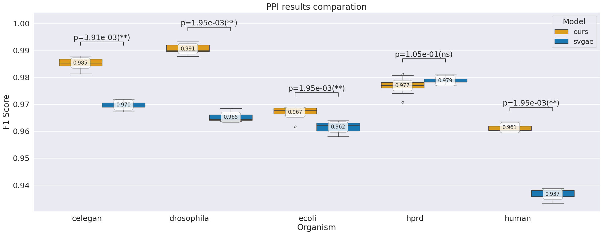
Figure 4: Comparison of the performance between our model and the SVGAE model across different organisms. Each boxplot represents the distribution of the F1 scores obtained from the 10 times 5-fold cross-validation. The boxplots show the mean F1 score for each k-fold, and the small box inside each plot indicates the overall mean F1 score across all k-folds. The p-value from the Wilcoxon signed-rank test is also indicated, showing the significance level of the difference between models.

To evaluate the performance of the proposed model, we compared it with the Signed Variational Graph Auto-Encoder (SVGAE) [22], a state-of-the-art approach specifically designed for protein-protein interaction (PPI) prediction. SVGAE has demonstrated significant accuracy improvements over traditional sequence-based methods and achieved leading performance on various datasets described in the corresponding section. SVGAE was selected as a benchmark due to its effective utilization of graph structures for capturing complex relationships in biological networks, aligning well with the edge-centric design of their model.

Figure 4 shows the F1 score performance of both models on each dataset. Each boxplot represents the distribution of F1 scores from the 10 repeated runs of 5-fold cross-validation, with boxplot pairs comparing our model to SVGAE on each dataset. As indicated by the Wilcoxon signed-rank test, our model significantly outperformed SVGAE on four datasets—C. elegans, Drosophila, E. coli, and Human—with notably low p-values (p $<$ 0.001). For the HPRD dataset, however, there was no significant difference in performance between the two models, suggesting comparable predictive accuracy in this specific case.

IV-B Gene Ontology (GO) term prediction

For this task, we compared our method against a baseline sequence approach used in the CAFA challenge [28, 35] (BLAST[36]) and three state-of-the-art approaches: NMF-GO [37], deepGOplus [38], and exp2GO [26]. Following the experimental setup used by NMF-GO and exp2GO, we trained on historical GOA files (2016) and validated predictions using the 2017 GOA file.

The 2016 dataset was split into training and validation sets (16% of the data) and the model was trained using the loss function described in Eq 7 and the same tokenizer architecture (linear, ReLU, linear, Tanh), applied when node features were available, as in the case of PPI prediction. The model was used to predict the semantic similarity matrix between genes, filling the gaps left because it was not possible to calculate semantic distances over the GO for unannotated genes. Early stopping with the validation set was performed by calculating the F1 score using a Bayesian probability method to predict the GO terms, as described in [26]. Five runs were performed with different initialization seeds, and the run with the lowest validation F1 score was selected. This approach efficiently evaluates the model’s ability to predict GO terms on newly annotated proteins.

Figure 6 presents a comparison of the different models across the datasets, organized into three subplots corresponding to the Molecular Function (MF), Biological Process (BP), and Cellular Component (CC) subontologies. Each subplot illustrates the performance of the models based on the $\text{F}1_{max}$ score across various species within the dataset, with the x-axis representing the different models and the y-axis indicating their respective $\text{F}1_{max}$ values. In the MF subontology, the performance among the models is closely matched, with the proposed model showing a slight improvement for the Dicty species. Moving to the BP subontology, although the proposed model does not outperform exp2go, it still performs commendably, reflecting its capability in this area. Finally, in the CC subontology, the proposed model demonstrates a slight advantage over the others, highlighting its overall effectiveness in predicting functional similarity across diverse biological contexts.

To conduct a statistical analysis of the results, the Friedman test and critical difference diagram [39], followed by the post-hoc Nemenyi test, were employed to assess the significance of the performance differences between the models.

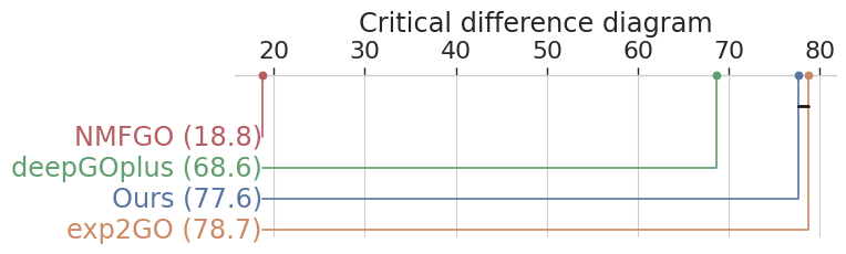
Figure 5: The critical difference (CD) diagram presents the statistical significance of the results. Models connected by a black line have no statistically significant difference. The CD value is 1.36.

The Friedman test results indicate that there are significant differences in the performance of the models being compared (p=$1e\!-\!6$). The critical difference diagram in Figure 5 shows that both the proposed model and exp2GO are the best methods for gene function prediction, with no statistically significant difference between them (p = $0.237$). However, there is a significant difference between the proposed model and deepGOplus (p = $1e\!-\!3$) as well as NMFGO (p = $1e\!-\!3$).

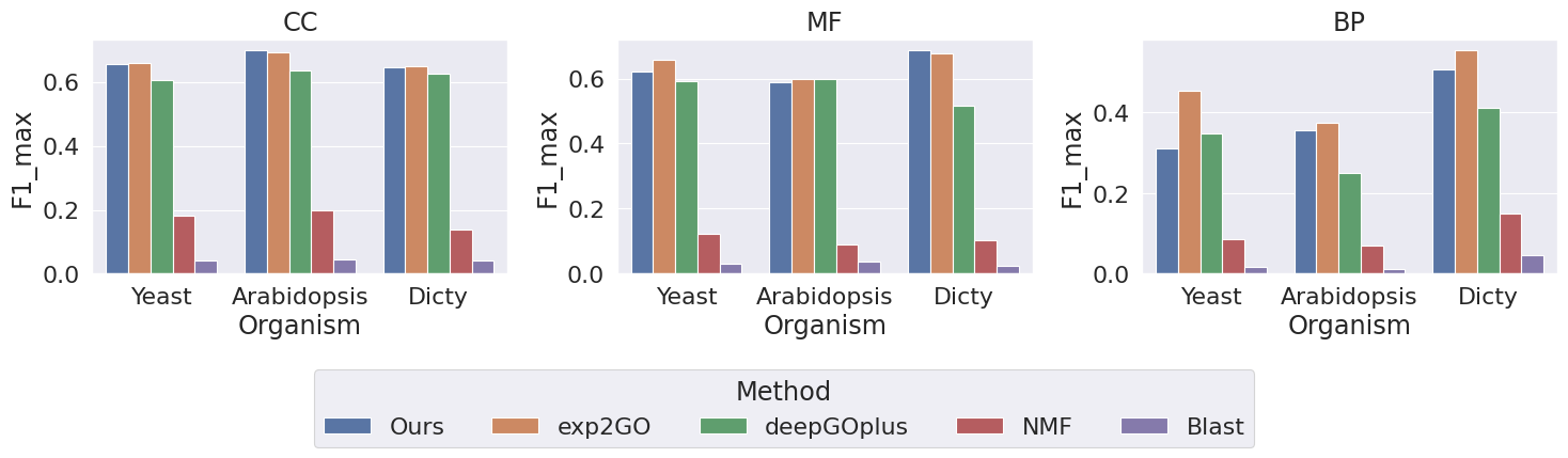
Figure 6: Bar plot comparing the maximum F1 scores of different models across each subontology (Cellular Component, Molecular Function, and Biological Process) for each organism. The plot highlights the performance of our model against other methods (exp2GO, deepGOplus, and NMFGO) across all subontologies and organisms.

IV-C Compounds similarity prediction

In this section, the findings on compound similarity are presented. While traditional approaches often rely on structural information, they face limitations when the compound structure is not available. We address this issue by using one-hot encoding as input features, enabling the model to predict similarity even in the absence of structural data.

For this task, the tokenizer employed a simpler architecture compared to previous experiments, consisting of a single linear layer followed by a Tanh activation function, effectively handling one-hot encoded features through extensive experimentation. Using this setup, we conducted a 5-fold cross-validation, obtaining a Mean Absolute Error (MAE) of 0.013. Given that the Tanimoto coefficient ranges from 0 to 1, this error represents only 1.3%, indicating a high degree of accuracy in our model’s predictions.

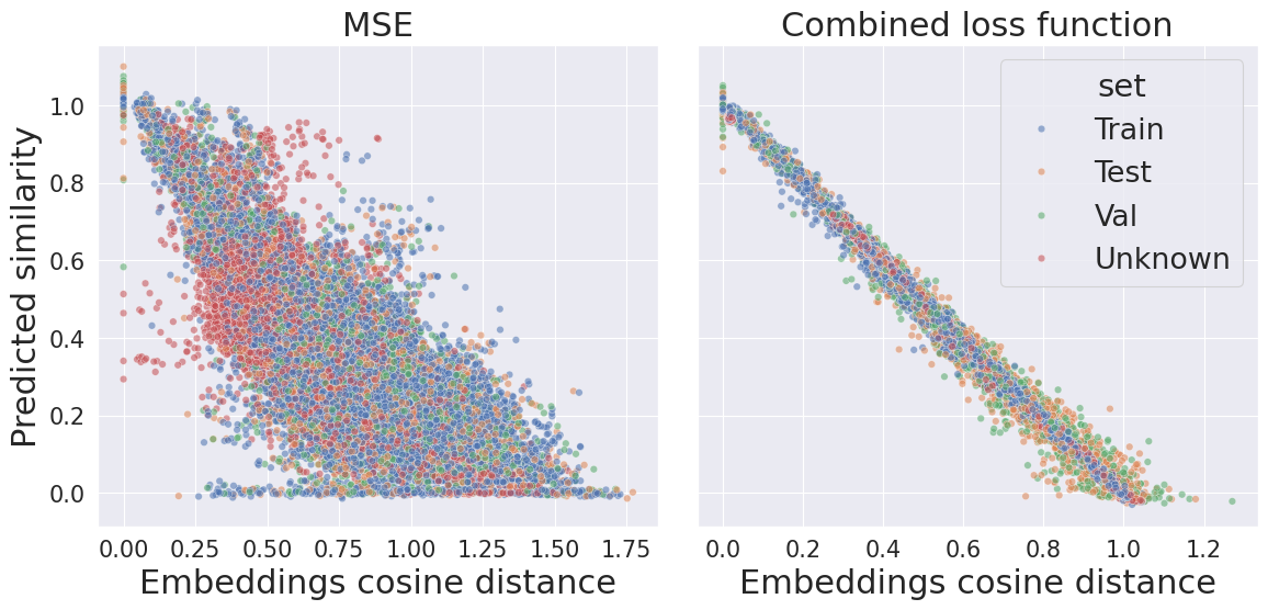
Figure 7: Comparison of embedding spatial distribution using MSE (right) and combined cost function (left). The combined cost function improves the linear relationship between compound similarity and cosine distance.

Figure 7 shows two subplots comparing predicted similarity (y-axis) to the cosine distance of embeddings (x-axis) under different cost functions. The right subplot displays results using our combined cost function, while the left shows the Mean Squared Error (MSE) approach. The combined cost function not only enhances the spatial organization of embeddings but also establishes a clearer linear relationship between compound similarity and cosine distance, facilitating accurate predictions. This arrangement enables both compounds with known and unknown structures to be effectively ordered within the embedding space, optimizing the predictor’s performance.

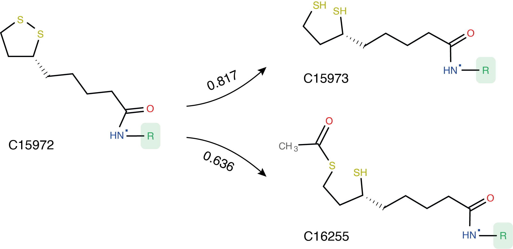
Figure 8: Partial structures of the compounds with KEGG ID C15972, C15973, and C16255. Generic substituents, marked in green as ’-R’, indicate that any functional group substituting for a hydrogen atom in the base compound structure, making it impossible to create a fingerprint for the compound. The arrows indicate predicted similarity values between compounds.

Figure 8 shows partial structures of the compounds with KEGG IDs C15972, C15973, and C16255. Although the molecular structures are partially known, each includes a generic substituent ’-R’, making it difficult to objectively assess similarity, as this information cannot be used to build fingerprints. This limitation, however, does not affect our approach, which instead represents compounds using embeddings learned from the graph topology of the metabolic pathway. For instance, our method predicts a similarity score of 0.817 between C15972 and C15973, which aligns with visual analysis as both compounds share a high proportion of their molecular structures. Similarly, a score of 0.636 between C15972 and C16255 reflects a moderate structural similarity, as these compounds share some structural elements but to a lesser extent than C15972 and C15973.

Figure 9 presents a PCA projection plot of the embeddings for the analyzed compounds into the first two principal components, learned using our loss function. In this plot, colors indicate similarity to a reference compound, glucose-1-P, marked in red. As we move away from this reference compound, similarity values decrease gradually, with colors transitioning towards violet. This gradient effectively captures the similarity relationships within the dataset.

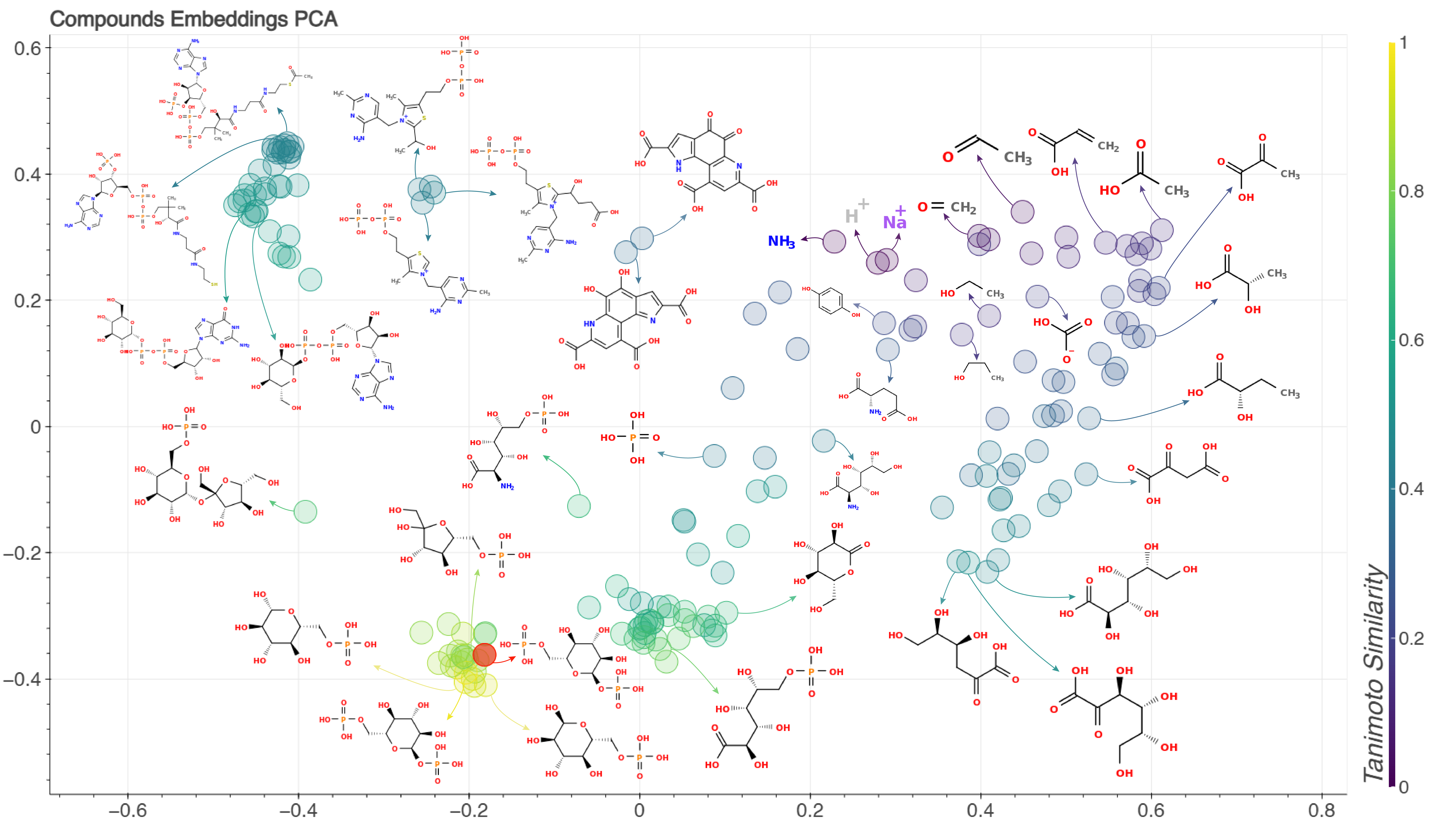
Figure 9: PCA plot of embeddings for the analyzed compounds. Colors represent similarity to a reference compound (glucose-1-P), indicated in red. Similarity values decrease (colors shift towards violet) as the distance from the reference compound increases. Additionally, some compounds are shown with their molecular structures.

V Conclusion

This study introduces a novel model based on Message Passing Neural Networks (MPNNs) designed to address edge-centric tasks in graph-based learning. By integrating an attention mechanism, the proposed architecture effectively utilizes both node features and edge attributes, enhancing its performance in edge regression and classification tasks where traditional methods have often faced limitations.

The custom loss function introduced in this model combines supervised and self-supervised learning, allowing it to optimize both predictions and embeddings simultaneously. This approach ensures robust generalization, even in scenarios with limited or missing information about nodes. By utilizing cosine similarity between node embeddings and predictions, the model effectively organizes learned representations, facilitating the modeling of complex relationships within dynamic graphs.

Experimental results across multiple datasets demonstrate that the proposed model outperforms state-of-the-art methods in protein-protein interaction (PPI) prediction while remaining competitive in Gene Ontology (GO) term prediction. The model also demonstrates that k-Nearest Neighbors Graphs (KNNG) based on node similarity measures are effective for graph construction, enhancing the model’s capacity to propagate information from neighboring nodes and enrich node descriptors.

Moreover, the model presents a novel solution to the problem of predicting similarity between compounds with unknown structure, using one-hot encoding as node features to compensate for the absence of detailed structural information. This approach not only enables accurate similarity predictions without requiring compound structure but also proves valuable in scenarios with limited or missing node features, generating meaningful representations even with sparse data. Its effectiveness in this area suggests potential applications in drug discovery, molecular similarity assessment, and similarity search.

In conclusion, the proposed model offers a flexible and powerful solution for a range of graph-based applications. Future research may focus on extending its capabilities to other fields of application, for example in recommendation systems, and social network analytics, among others that may benefit from the capabilities of predicting properties of pairs of nodes. In all our experiments we have used a one-layer MPNN, but we need to explore the possibility of using additional layers of MPNN in the Embedder section. Furthermore, future investigations will consider methods to generate predictions with associated uncertainty intervals, providing a measure of confidence in the model’s predictions.

References

- [1] S. P. Tiwari, “Social Media Based Recommender System for E- Commerce Platforms,” International Journal of Research in Engineering and Science (IJRES), pp. 87–98, 2021.
- [2] H. Steck, L. Baltrunas, E. Elahi, D. Liang, Y. Raimond, and J. Basilico, “Deep Learning for Recommender Systems: A Netflix Case Study,” AI Magazine, vol. 42, no. 3, pp. 7–18, Nov. 2021, number: 3.
- [3] P. Covington, J. Adams, and E. Sargin, “Deep Neural Networks for YouTube Recommendations,” in Proceedings of the 10th ACM Conference on Recommender Systems. Boston Massachusetts USA: ACM, Sep. 2016, pp. 191–198.
- [4] Z. Wu, S. Pan, F. Chen, G. Long, C. Zhang, and P. S. Yu, “A comprehensive survey on graph neural networks,” IEEE transactions on neural networks and learning systems, vol. 32, no. 1, pp. 4–24, 2020.
- [5] M. E. Newman, “The structure and function of complex networks,” SIAM Review, vol. 45, pp. 167–256, 3 2003.
- [6] B. Perozzi, R. Al-Rfou, and S. Skiena, “DeepWalk: Online Learning of Social Representations,” in Proceedings of the 20th ACM SIGKDD international conference on Knowledge discovery and data mining, Aug. 2014, pp. 701–710, arXiv:1403.6652 [cs].
- [7] J. Tang, M. Qu, M. Wang, M. Zhang, J. Yan, and Q. Mei, “Line: Large-scale information network embedding,” in Proceedings of the 24th International Conference on World Wide Web, ser. WWW ’15, vol. 14. International World Wide Web Conferences Steering Committee, May 2015, p. 1067–1077.
- [8] A. Grover and J. Leskovec, “node2vec: Scalable Feature Learning for Networks,” in Proceedings of the 22nd ACM SIGKDD International Conference on Knowledge Discovery and Data Mining. San Francisco California USA: ACM, Aug. 2016, pp. 855–864.
- [9] W. L. Hamilton, R. Ying, and J. Leskovec, “Representation learning on graphs: Methods and applications,” 9 2017.
- [10] J. Zhou, G. Cui, S. Hu, Z. Zhang, C. Yang, Z. Liu, L. Wang, C. Li, and M. Sun, “Graph neural networks: A review of methods and applications,” AI Open, vol. 1, pp. 57–81, 2020.
- [11] J. Bruna, W. Zaremba, A. Szlam, and Y. LeCun, “Spectral networks and locally connected networks on graphs,” arXiv preprint arXiv:1312.6203, 2013.
- [12] M. Defferrard, X. Bresson, and P. Vandergheynst, “Convolutional neural networks on graphs with fast localized spectral filtering,” in Advances in neural information processing systems, 2016, pp. 3844–3852.
- [13] D. I. Shuman, S. K. Narang, P. Frossard, A. Ortega, and P. Vandergheynst, “The emerging field of signal processing on graphs: Extending high-dimensional data analysis to networks and other irregular domains,” IEEE Signal Processing Magazine, vol. 30, pp. 83–98, 2013.
- [14] X. Zhu and M. Rabbat, “Approximating signals supported on graphs,” ICASSP, IEEE International Conference on Acoustics, Speech and Signal Processing - Proceedings, pp. 3921–3924, 2012.
- [15] M. M. Bronstein, J. Bruna, Y. LeCun, A. Szlam, and P. Vandergheynst, “Geometric deep learning: going beyond euclidean data,” 11 2016.
- [16] Z. Wu, S. Pan, F. Chen, G. Long, C. Zhang, and P. S. Yu, “A comprehensive survey on graph neural networks,” 2019.
- [17] Z. Zhang, P. Cui, and W. Zhu, “Deep learning on graphs: A survey,” 2020.
- [18] J. Gilmer, S. S. Schoenholz, P. F. Riley, O. Vinyals, and G. E. Dahl, “Message passing neural networks,” Lecture Notes in Physics, vol. 968, pp. 199–214, 2020.
- [19] D. K. Duvenaud, D. Maclaurin, J. Iparraguirre, R. Bombarell, T. Hirzel, A. Aspuru-Guzik, and R. P. Adams, “Convolutional networks on graphs for learning molecular fingerprints,” in Advances in neural information processing systems, 2015, pp. 2224–2232.
- [20] S. Kearnes, K. McCloskey, M. Berndl, V. Pande, and P. Riley, “Molecular graph convolutions: moving beyond fingerprints,” Journal of computer-aided molecular design, vol. 30, pp. 595–608, 2016.
- [21] A. Vaswani, N. Shazeer, N. Parmar, J. Uszkoreit, L. Jones, A. N. Gomez, Łukasz Kaiser, and I. Polosukhin, “Attention is all you need,” Advances in Neural Information Processing Systems, vol. 2017-December, pp. 5999–6009, 6 2017.
- [22] F. Yang, K. Fan, D. Song, and H. Lin, “Graph-based prediction of protein-protein interactions with attributed signed graph embedding,” BMC Bioinformatics, vol. 21, pp. 1–16, 7 2020.
- [23] F. Sievers, A. Wilm, D. Dineen, T. J. Gibson, K. Karplus, W. Li, R. Lopez, H. McWilliam, M. Remmert, J. Söding, J. D. Thompson, and D. G. Higgins, “Fast, scalable generation of high-quality protein multiple sequence alignments using clustal omega,” Molecular Systems Biology, vol. 7, p. 539, 2011.
- [24] R. Paredes, E. Chávez, K. Figueroa, and G. Navarro, “Practical construction of k-nearest neighbor graphs in metric spaces,” Lecture Notes in Computer Science (including subseries Lecture Notes in Artificial Intelligence and Lecture Notes in Bioinformatics), vol. 4007 LNCS, pp. 85–97, 2006.
- [25] J. Shen, J. Zhang, X. Luo, W. Zhu, K. Yu, K. Chen, Y. Li, and H. Jiang, “Predicting protein-protein interactions based only on sequences information,” Proceedings of the National Academy of Sciences of the United States of America, vol. 104, pp. 4337–4341, 3 2007.
- [26] L. D. Persia, T. Lopez, A. Arce, D. H. Milone, and G. Stegmayer, “exp2go: Improving prediction of functions in the gene ontology with expression data,” IEEE/ACM transactions on computational biology and bioinformatics, vol. 20, pp. 999–1008, 3 2023.
- [27] M. B. Eisen, P. T. Spellman, P. O. Brown, and D. Botstein, “Cluster analysis and display of genome-wide expression patterns,” Proceedings of the National Academy of Sciences of the United States of America, vol. 95, pp. 14 863–14 868, 12 1998.
- [28] N. Zhou, Y. Jiang, T. R. Bergquist, A. J. Lee, B. Z. Kacsoh, A. W. Crocker, K. A. Lewis, G. Georghiou, H. N. Nguyen, M. N. Hamid, L. Davis, T. Dogan, V. Atalay, A. S. Rifaioglu, A. Dalklran, R. C. Atalay, C. Zhang, R. L. Hurto, P. L. Freddolino, Y. Zhang, P. Bhat, F. Supek, J. M. Fernández, and B. Gemovic, “The cafa challenge reports improved protein function prediction and new functional annotations for hundreds of genes through experimental screens,” Genome Biology, vol. 20, pp. 1–23, 11 2019.
- [29] C. Espinoza, T. Degenkolbe, C. Caldana, E. Zuther, A. Leisse, L. Willmitzer, D. K. Hincha, and M. A. Hannah, “Interaction with diurnal and circadian regulation results in dynamic metabolic and transcriptional changes during cold acclimation in arabidopsis,” PloS one, vol. 5, 2010.
- [30] L. Kreppel, P. Fey, P. Gaudet, E. Just, W. A. Kibbe, R. L. Chisholm, and A. R. Kimmel, “dictybase: a new dictyostelium discoideum genome database,” Nucleic acids research, vol. 32, 1 2004.
- [31] E. Borzone, L. E. Di Persia, and M. Gerard, “Neural model-based similarity prediction for compounds with unknown structures,” in Applied Informatics, H. Florez and H. Gomez, Eds. Cham: Springer International Publishing, 2022, pp. 75–87.
- [32] E. Borzone, L. Ezequiel, D. Persia, and M. Gerard, “Evaluación de un modelo neuronal para la estimación de similaridad entre compuestos a partir de representaciones one-hot,” 2022.
- [33] J. L. Durant, B. A. Leland, D. R. Henry, and J. G. Nourse, “Reoptimization of mdl keys for use in drug discovery,” Journal of chemical information and computer sciences, vol. 42, pp. 1273–1280, 11 2002.
- [34] D. Bajusz, A. Rácz, and K. Héberger, “Why is tanimoto index an appropriate choice for fingerprint-based similarity calculations?” Journal of Cheminformatics, vol. 7, pp. 1–13, 12 2015.
- [35] P. Radivojac, W. T. Clark, T. R. Oron, A. M. Schnoes, and T. Wittkop, “A large-scale evaluation of computational protein function prediction,” Nature Methods 2013 10:3, vol. 10, pp. 221–227, 1 2013.
- [36] S. F. Altschul, W. Gish, W. Miller, E. W. Myers, and D. J. Lipman, “Basic local alignment search tool,” Journal of molecular biology, vol. 215, pp. 403–410, 1990.
- [37] G. Yu, K. Wang, G. Fu, M. Guo, and J. Wang, “Nmfgo: Gene function prediction via nonnegative matrix factorization with gene ontology,” IEEE/ACM transactions on computational biology and bioinformatics, vol. 17, pp. 238–249, 1 2020.
- [38] M. Kulmanov and R. Hoehndorf, “Deepgoplus: improved protein function prediction from sequence,” Bioinformatics (Oxford, England), vol. 36, pp. 422–429, 1 2020.
- [39] DemšarJanez, “Statistical comparisons of classifiers over multiple data sets,” The Journal of Machine Learning Research, vol. 7, pp. 1–30, 12 2006.