Systematic Abductive Reasoning via Diverse Relation Representations in Vector-symbolic Architecture

Abstract

In abstract visual reasoning, monolithic deep learning models suffer from limited interpretability and generalization, while existing neuro-symbolic approaches fall short in capturing the diversity and systematicity of attributes and relation representations. To address these challenges, we propose a Systematic Abductive Reasoning model with diverse relation representations (Rel-SAR) in Vector-symbolic Architecture (VSA) to solve Raven’s Progressive Matrices (RPM). To derive attribute representations with symbolic reasoning potential, we introduce not only various types of atomic vectors that represent numeric, periodic and logical semantics, but also the structured high-dimentional representation (SHDR) for the overall Grid component. For systematic reasoning, we propose novel numerical and logical relation functions and perform rule abduction and execution in a unified framework that integrates these relation representations. Experimental results demonstrate that Rel-SAR achieves significant improvement on RPM tasks and exhibits robust out-of-distribution generalization. Rel-SAR leverages the synergy between HD attribute representations and symbolic reasoning to achieve systematic abductive reasoning with both interpretable and computable semantics.

I Introduction

Raven’s Progressive Matrices (RPM) are a family of psychological intelligence tests widely used for the assessment of abstract reasoning [carpenter1990one, bilker2012development]. From a cognitive psychology perspective, abstract visual reasoning in RPM tests involves constructing high-level representations from images and deriving potential relations from these representations [carpenter1990one, mitchell2021abstraction]. Endowing artificial intelligence with such capabilities is now regarded as a crucial step toward achieving human-level intelligence. However, many recent monolithic deep learning models, which do not explicitly separate perception and reasoning [barrett2018measuring, hill2019learning, zhang2019learning, zheng2019abstract, hu2021stratified, benny2021scale], face inherent challenges, such as poor interpretability, limited robustness and generalization, and difficulties in module reuse [zhang2021abstract]. Neuro-symbolic architecture, which combines neural visual perception with symbolic reasoning, offers a promising approach to overcoming these challenges and achieving human-level interpretability and generalization [marcus2003algebraic, zhang2021abstract, hersche2023neuro].

In neuro-symbolic architectures (NSA), Marcus argues that symbol-manipulation in cognition involves representing relations between variables [marcus2003algebraic]. For RPM tests, object attributes serve as the variables, while potential rules involve the relations. Nevertheless, due to incomplete attribute and relation representations, achieving systematic abduction and execution is still a critical challenge for NSA when performing RPM tests. From the perspective of attributes, recent models such as PrAE [zhang2021abstract], the ALANS learner [zhang2022learningb], and NVSA (neuro-vector-symbolic architecture) [hersche2023neuro] construct attribute representations through neural perception frontends. Notably, the NVSA model achieves hierarchically structured VSA representations of image panels, capturing multiple objects with multiple attributes [hersche2023neuro]. Regarding relation representations, PrAE and NVSA achieve abstract reasoning through probabilistic abduction and execution [zhang2021abstract] and distributed vector-symbolic architecture (VSA) [hersche2023neuro], respectively. Both models rely on predetermined multiple rule templates, each specialized for distinct individual RPM rules. To address the limitations in rule expressiveness, the ALANS learner utilizes learnable rule operators in the abstract algebraic structure, without manual definition for every rules [zhang2022learningb]. Additionally, the ARLC model adopts a more expressive VSA-based rule template, operating in the rule parameter space [camposampiero2024towards]. Both models offer improved interpretabiltiy and generalizability. Despite their advances, previous models fall short in capturing the diversity and systematicity of attribute and relation representations. In contrast, human cognition demonstrates rich and flexible internal representations [mansouri2020emergence, marcus2020insights], including arithmetic and logic, and rule-based reasoning systems in cognition are productive and systematic [sloman1996empirical]. Therefore, the abstract visual reasoning performance of these models remains open to further improvement.

Previous research indicates that Vector Symbolic Architecture (VSA), a form of high-dimensional (HD) distributed representation, possesses algebraic properties for mathematical operations and can also achieve structured symbolic representations of data [plate1994distributed, Frady_Kleyko_Kymn_Olshausen_Sommer_2021, kleyko2022survey]. In this work, to achieve comprehensive relation representations, we introduce various types of VSA-based atomic HD vectors with distinct semantic representations, including numeric values, periodic values, and logical values. Given that reasoning in RPM problems involves the overall attributes of multiple objects, we further introduce the structured HD representation (SHDR) for the nxn Grid. They serve as attribute representations necessary for abductive reasoning. Meanwhile, we propose numerical and logical relation functions as relation representations that take multiple HD attribute representations as input and define relations among them. Unlike rule templates designed for individual rules, the two proposed relation functions are specifically tailored to numerical and logical types, providing strong rule expressiveness.

Here, we propose a Systematic Abductive Reasoning model with diverse relation representations (Rel-SAR) for solving RPM, inspired by the original NVSA model [hersche2023neuro]. In the Rel-SAR model, visual attribute extraction and rule inference are implemented within a fully unified computational framework in the VSA machinery. The model comprises a neuro-vector frontend for perceiving object attributes of all raw images in RPM problems and a generic vector-symbolic backend for achieving symbolic reasoning. The perception frontend operates on scene-based SHDR of each image panel, which contains multiple objects, each with various attributes, and predicts HD attribute representations by VSA-based symbolic manipulations. The reasoning backend implements the core idea of systematic abductive reasoning: if the given attributes in an RPM adhere to a specific numerical or logical rule, then the relation representations of all attribute pairs can be defined using the corresponding relation functions with identical parameters. These diverse relation representations are involved in both rule abduction and execution phases, enhancing interpretability and improving the capacity for systematic abductive reasoning.

II Related Work

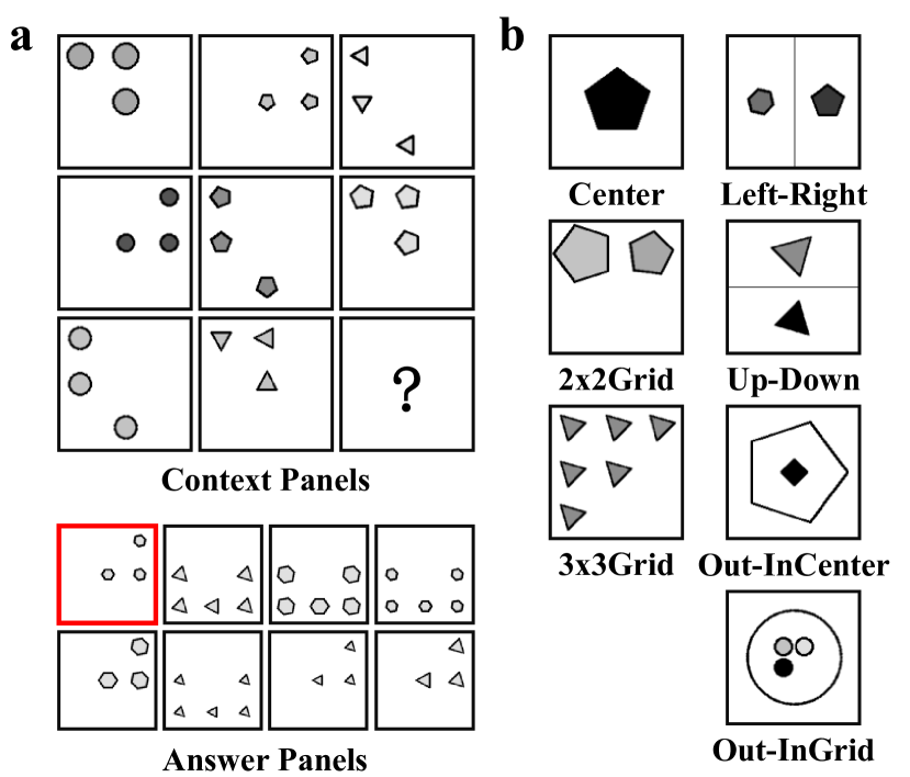
Figure 1: Illustrations for RAVEN dataset. (a) An example of RPM test from RAVEN[zhang2019raven] dataset. In an RPM test, there are 8 context panels and 8 candidate panels. Participants are required to identify the underlying rules governing various attributes within the context panels. Subsequently, participants use these rules to infer the attributes of the missing panel (represented by ”?”) and choose the most appropriate option (highlighted with a red box) from the answer panels. (b) The RAVEN dataset includes seven configurations: Center, 2x2Grid, 3x3Grid, Left-Right (L-R), Up-Down (U-D), Out-InCenter (O-IC) and Out-InGrid (O-IG) [zhang2019raven]. Four types of rules, i.e., Constant, Progression, Arithmetic, and Distribute Three, are applied to five attributes, i.e., Position, Number, Type, Size, and Color, in a row-wise manner. The I-RAVEN dataset [hu2021stratified] is a variant of RAVEN, where answer sets are generated using an attribute bisection tree.

The Raven Progressive Matrices (RPM) is a widely used nonverbal intelligence test designed to assess abstract reasoning. To explore the limitations of current machine learning approaches in solving abstract reasoning tasks, two automatically generated RPM-based datasets—RAVEN [zhang2019raven] and I-RAVEN [hu2021stratified]—have been introduced (Figure 1). Early efforts on RPM primarily employed Relation Network (RN) [santoro2017simple] and their variants [barrett2018measuring, jahrens2020solving, zheng2019abstract, benny2021scale] to extract relations between context panels. Concurrently, CoPINet [zhang2019learning], MLCL [malkinski2022multi], and DCNet [zhuo2022effective] integrate contrastive learning in their models. Approaches like MRNet [benny2021scale] and DRNet [zhao2024learning] aimed to enhance perception capabilities, while SRAN [hu2021stratified] and PredRNet [yang2023neural] abstract relations using stratified models and prediction errors, respectively. In addition, several methods have focused on scene decomposition and feature disentanglement [wu2020scattering, mondal2023learning, spratley2020closer]. Although these monolithic deep learning models achieve high accuracy, they often suffer from limited interpretability and systematic generalization capabilities.

Another branch for solving RPM is based on neuro-symbolic architectures, which explicitly distinguish between perception and reasoning. PrAE [zhang2021abstract] employs an object CNN to generate probabilistic scene representations and uses predetermined rule templates for probabilistic abduction and execution. Inspired by abstract algebra and representation theory, ALANS [zhang2022learningb], which shares the same perception frontend as PrAE, transforms probabilistic scene distributions into matrix-based algebraic representations. The algebraic reasoning backend of ALANS induces potential rules through trainable operator matrices, eliminating the need for manual rule definitions. In abstract reasoning, Vector Symbolic Architectures (VSA) serve as a bridge between perception and reasoning modules by leveraging its structured distribution representations and algebraic properties. NVSA [hersche2023neuro] projects each RPM panel into a high-dimensional vector using a trainable CNN and derives probability mass functions (PMFs) by querying an external codebook. Its reasoning backend embeds these PMFs into distributed VSA representations and performs rule abduction and execution using templates based on VSA algebraic operations. NVSA provides a differentiable and transparent implementation of probabilistic abductive reasoning by leveraging VSA representations and operators. However, its perception frontend requires searching a large external codebook, and its reasoning backend still relies on predetermined rule templates. In contrast, Learn-VRF [hersche2024probabilistic], focuses on reasoning by learning VSA rule formulations, eliminating the need for predetermined templates. ARLC [camposampiero2024towards] further enhances reasoning by incorporating context augmentation and extending rule templates to accommodate more diverse rules. While ARLC and Learn-VRF implement systematic rule learning, they still struggle to process all RPM rules due to limitations in attribute representation. Recently, a class of methods known as relational bottlenecks has been proposed to enable efficient abstraction, but their capacity to handle complex relations remains uncertain[webb2020emergent, altabaa2023abstractors, kerg2022neural, webb2024relational]. To address this limitation, Rel-SAR transforms perceptual inputs into high-dimensional attribute representations with symbolic reasoning potential and abducts both logical and numerical rules within a unified framework.

III Preliminaries

III-A VSA models utilized in this study

VSAs are a class of computational models that utilize high-dimensional distributed representations [kleyko2022survey]. VSA models used in this study are Holographic Reduced Representations (HRR) and its form in the frequency domain, referred to as Fourier Holographic Reduced Representations (FHRR)[plate1995holographic]. A random FHRR atomic vector, denoted as $\boldsymbol{\theta}:=\left\{\theta_{i}\right\}_{i=1}^{d}$, is composed of elements $\theta_{i}$ that are independently sampled from a uniform distribution, specifically $\theta_{i}\sim\mathcal{U}(-\pi,\pi)$ [plate1995holographic]. The corresponding HRR atomic vector, $\boldsymbol{x}$, is then obtained by applying the Inverse Fast Fourier Transform (IFFT) to $\boldsymbol{\theta}$:

$$\boldsymbol{x}=\mathcal{F}^{-1}\left(e^{j\boldsymbol{\theta}}\right)$$ (1)

Here, $\mathcal{F}$ and $\mathcal{F}^{-1}(\cdot)$ represent the Fast Fourier Transform (FFT) and Inverse FFT (IFFT), respectively. When the dimension $d$ is sufficiently large, these randomly generated vectors exhibit pseudo-orthogonality, making them suitable for representing distinct symbols or concepts.

The similarity between any two vectors is a crucial metric for evaluating the distributed representations in VSAs. In FHRR and HRR, cosine similarity is employed to measure the similarity between two vectors [kleyko2022survey]:

$$\begin{split}sim(\boldsymbol{\theta},\boldsymbol{\phi})&=\frac{1}{d}\sum_{i=1}^{d}{\cos\left(\theta_{i}-\varphi_{i}\right)}\\ sim(\boldsymbol{x},\boldsymbol{y})&=\frac{\boldsymbol{x}\cdot\boldsymbol{y}}{\left|\boldsymbol{x}\right|\left|\boldsymbol{y}\right|}\end{split}$$ (2)

where $\boldsymbol{\theta}$ and $\boldsymbol{\phi}$ denote two FHRR vectors, and $\boldsymbol{x}$ and $\boldsymbol{y}$ two HRR vectors. The similarity $sim(\cdot,\cdot)$ ranges from -1 to +1, and above two similarity measures are equivalent. The pseudo-orthogonality refers to the case where the similarity $sim(\cdot,\cdot)\approx 0$.

III-B Basic operations and structured symbolic representations

All computations within VSAs are composed of several basic vector algebraic operations, with the primary ones being binding ($\circ$), bundling ($+$) and unbinding ($\oslash$) (Table I). The binding operation ($\circ$) is employed to form a representation of an object that contains information about the context in which it was encountered [kleyko2022survey]. The bundling operation ($+$), also known as superposition, generates a composite high dimensional vector that combines several lower-level representations. In calculation, binding has a higher priority than bundling. The unbinding operation ($\oslash$), which is the inverse of binding, extracts a constituent from the compound data structure. Binding and bundling are referred to as composition operations, while unbinding is considered a decomposition operation. All operations do not change the vector dimensionality.

Through the combination of these operations, VSAs can effectively achieve structured symbolic representations [kleyko2022survey]. For instance, consider a scene $\boldsymbol{s}$ in which a triangle $\boldsymbol{t}$ is positioned on the left $\boldsymbol{p}_{L}$ and a circle $\boldsymbol{c}$ on the right $\boldsymbol{p}_{R}$. This scene can be represented as $\boldsymbol{s}=\boldsymbol{p}_{L}\circ\boldsymbol{t}+\boldsymbol{p}_{R}\circ\boldsymbol{c}$ by the role-filler pair [kanerva2009hyperdimensional]. By applying the inverse vector of the left position $\boldsymbol{p}_{L}^{-1}$ to unbind $\boldsymbol{s}$, we can retrieve an approximate vector representing the content at the left position, i.e., $\boldsymbol{p}_{L}^{-1}\otimes\boldsymbol{s}\approx\boldsymbol{t}$. Moreover, the triangle $\boldsymbol{t}$ can itself be a compositional scene, where attributes such as color and size are combined into a triangle scene in a similar manner. This decomposable, structure-sensitive, high-dimensional distributed representation has the potential to disentangle complex scenes while maintaining the advantages of traditional connectionist approaches [hersche2023neuro].

III-C The fractional power encoding method

In this study, the rules in RPM are primarily numerical. We introduce the VSA representation of numerical values using the fractional power encoding method (FPE-VSA) [plate1994distributed, Frady_Kleyko_Kymn_Olshausen_Sommer_2021]. Let $x\in\mathbb{R}$ be a real number and $X\in\mathbb{R}^{d}$ a randomly sampled base vector. The VSA representation $\boldsymbol{v}(x)\in\mathbb{R}^{d}$ for any value $x$ is obtained by repeatedly binding the base vector $X$ with itself $x$ times, as follows:

$$\boldsymbol{v}\left(x\right):=\left(X\right)^{\left(\circ x\right)}$$ (3)

The FPE method maps arbitrary real numbers to corresponding HD vector, and has the following properties:

$$\boldsymbol{v}\left(x_{1}+x_{2}\right)=\boldsymbol{v}\left(x_{1}\right)\circ\boldsymbol{v}\left(x_{2}\right)$$ (4)

This demonstrates that addition $+$ in the real number domain can be represented by the binding operation $\circ$ in the vector domain.

TABLE I: Basic oprations of FHRR and HRR.

Operations	Impl. on FHRR	Impl. on HRR
Binding($\boldsymbol{x}\circ\boldsymbol{y}$)	$\left(\boldsymbol{\theta}+\boldsymbol{\phi}\right)mod\,\,2\pi$	$\mathcal{F}^{-1}\left(\mathcal{F}\left(\boldsymbol{x}\right)\cdot\mathcal{F}\left(\boldsymbol{y}\right)\right)$
Bundling($\boldsymbol{x}+\boldsymbol{y}$)	$angle\left(e^{j\boldsymbol{\theta}}+e^{j\boldsymbol{\phi}}\right)$	$\boldsymbol{x}+\boldsymbol{y}$
Inverse($\boldsymbol{x}^{-1}$)	$\left(-\boldsymbol{\theta}\right)\,\,mod\,\,2\pi$	$\mathcal{F}^{-1}\left(1/\mathcal{F}\left(\boldsymbol{x}\right)\right)$
Unbinding($\boldsymbol{x}\oslash\boldsymbol{y}$)	$\boldsymbol{\theta^{-1}}\circ\boldsymbol{\phi}$	$\boldsymbol{x^{-1}}\otimes\boldsymbol{y}$

IV Methodology

IV-A Atomic HD vectors with semantic representations

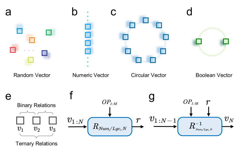
Figure 2: Atomic HD representations and relation functions. (a-d) The Rel-SAR model utilizes four types of atomic HD vectors. Random Vectors (RVs), sampled independently, are used to represent distinct and unrelated symbols or concepts. Numeric Vectors (NVs) are used to represent real numbers and support VSA-based addition-type arithmetic operations. Circular Vectors (CVs) represent periodic values and enable addition-type arithmetic operations with periodicity. Boolean Vectors (BVs), representing logical values of False and True, support VSA operations for logical reasoning. (e) In the RAVEN dataset, for a given attribute, the HD attribute representations in a row of three image panels involve binary or ternary relations. (f) Relation functions describe the numerical or logical relations between multiple HD vector representations $\boldsymbol{v}_{1:N}$, where $N=2$ for binary and $N=3$ for ternary relations. These relations are governed by the operator powers $OP_{1:M}$ and the output $\boldsymbol{r}$. (g) For a given relation defined by $OP_{1:M}$ and $\boldsymbol{r}$, inverse relation functions infer the last HD vector representation $\boldsymbol{v}_{N}$ according to the first $N-1$ representations $\boldsymbol{v}_{1:N-1}$.

In neuro-vector-symbolic systems, atomic HD vector representations with meaningful semantics are essential for perception and reasoning. We introduce four types of atomic HD vectors used in our model (Figure 2): Random Vectors (RVs), Numeric Vectors (NVs), Circular Vectors (CVs), and Boolean Vectors (BVs). The definitions and properties of these vectors are universal within the VSA framework.

IV-A1 Random Vector

RVs are sampled from specific distributions according to the VSA models, as mentioned in the preliminary section. Due to the absence of numerical or logical relations among RVs and their pseudo-orthogonality in the HD vector space (Figure 2a), they are often used to represent symbols and concepts assumed to be independent and dissimilar.

IV-A2 Numeric Vector

NVs, generated using the fractional power encoding (FPE-VSA, Equation 3) [plate1994distributed], are employed to represent real numbers (Figure 2b). NVs $\boldsymbol{v}(r)\in\mathbb{R}^{d}$ can be used to perform addition-type arithmetic operations through the binding (Equation 4) [Frady_Kleyko_Kymn_Olshausen_Sommer_2021].

IV-A3 Circular Vector

CVs are a special class of NVs used to represent periodic values (Figure 2c). Given a base vector $P$, where each phase of its elements $\rho_{i}$ is sampled from a discrete distribution ( e.g., for FHRR, $\rho_{i}\sim\mathcal{U}\left(2\pi j/L,\forall j\in\left\{1,\cdots,L\right\}\right)$, with $L$ being an even number), CVs are defined as $\boldsymbol{p}(r):=(P)^{(\circ r)}$. These CVs are pseudo-orthogonal to one another and exhibit periodicity with a period of $L$ [Frady_Kleyko_Kymn_Olshausen_Sommer_2021]:

$$\boldsymbol{p}\left(r+L\right)=\boldsymbol{p}\left(r\right)$$ (5)

If $L$ is odd, the corresponding CVs with period $L$ can be obtained by selecting every other CV from those with period $2L$.

IV-A4 Boolean Vector

BVs are a specific type of CVs with a period of $L=2$, used to represent Boolean values (Figure 2d). Following a similar generation method as for CVs, we can generate vectors with a period of $L=2$, $\boldsymbol{e}\left(0\right)$ and $\boldsymbol{e}\left(1\right)$, to represent False and True, respectively. Basic logic operations using BVs are implemented as shown in Table II, where $\boldsymbol{a},\boldsymbol{b}\in\{\boldsymbol{e}(0),\boldsymbol{e}(1)\}$ represent arbitrary Boolean values.

TABLE II: Logic operations implemented by BV

Operation	Implementation on BV
NOT	$\lnot\boldsymbol{a}=\boldsymbol{a}\circ\boldsymbol{e}\left(1\right)$
XOR	$\boldsymbol{a}\oplus\boldsymbol{b}=\boldsymbol{a}\circ\boldsymbol{b}$
AND	$\boldsymbol{a}\land\boldsymbol{b}=\boldsymbol{a}^{\left(\circ sim\left(\boldsymbol{a},\boldsymbol{b}\right)\right)}$
OR	$\begin{aligned} \boldsymbol{a}\lor\boldsymbol{b}&=\left(\boldsymbol{a}\oplus\boldsymbol{b}\right)\circ\left(\boldsymbol{a}\land\boldsymbol{b}\right)\\ \,\,&=\boldsymbol{a}\circ\boldsymbol{b}\circ\boldsymbol{a}^{\left(\circ sim\left(\boldsymbol{a},\boldsymbol{b}\right)\right)}\\ \end{aligned}$

IV-B Relation functions based on atomic HD representations

The rules for abductive reasoning in RPM involve binary and ternary relations among the attributes of corresponding objects in each row of three panels (Figure 2e and Figure 1a), as well as numerical and logical relations. In this work, we design general relation functions based on VSA algebra, utilizing the aforementioned atomic vector representations, to be used for rule abductions.

IV-B1 Relation functions

Relation functions, which describe the relations between multiple HD vector representations, are categorized into two types: numerical and logical. Among the atomic HD representations, Numeric Vectors (NVs) and Circular Vectors (CVs) are involved in numerical relations, while Boolean Vectors (BVs) are involved in logical relations.

The numerical relation function, $R_{Num}$, is defined as follows (Figure 2f):

$$\boldsymbol{r}_{Num}=R_{Num}\left(\boldsymbol{v}_{1:N},OP_{1:M}\right)=\circ_{i=1}^{N}\boldsymbol{v}_{i}^{\left(\circ op_{i}\right)}$$ (6)

where $N$ represents the arity of the relation function, and $\boldsymbol{v}_{1:N}:=\left\{\boldsymbol{v}_{i}\right\}_{i=1}^{N}$ denotes the input set of HD vector representations. $M$ is the number of operator powers and $OP_{1:M}:=\left\{op_{i}\right\}_{i=1}^{M}$ represents the operator powers, which can be considered as parameters of the relation function. The notation $\circ_{i=1}^{N}$ denotes the sequential binding operation applied to the $N$ HD vector representations. $\boldsymbol{r}_{Num}$ is the output HD representation. For the binary numerical relation function, $N=2$ and $M=2$, while for the ternary numerical relation function, $N=3$ and $M=3$. Based on the arithmetic properties of NVs and CVs, $R_{Num}$ can describe the additive relations of these two types of HD vector representations. The combination of $OP_{1:M}$ and $\boldsymbol{r}_{Num}$ determines the specific numerical relation in this vector-symbolic method.

Similarly, the simplified logical relation function, $R_{Lgc}$, is defined as follows (Figure 2f):

$$\boldsymbol{r}_{Lgc}=R_{Lgc}\left(\boldsymbol{v}_{1:N},OP_{1:M}\right)=\left(op_{1}\boldsymbol{v}_{1}\land op_{2}\boldsymbol{v}_{2}\right)\circ op_{3}\boldsymbol{v}_{3}$$ (7)

where $\boldsymbol{v}_{1:N}:=\left\{\boldsymbol{v}_{i}\right\}_{i=1}^{N}\in\{\boldsymbol{e}(0),\boldsymbol{e}(1)\}$ denotes the input set of BVs. The full version of logical relation function is described in Appendix LABEL:sec:appendix_1. Here, we consider only the ternary logical relation, so $N=3$ and $M=3$. The parameter $OP_{1:M}:=\left\{op_{i}\right\}_{i=1}^{M}$, where $op_{i}\in\{0,1\}$ determines whether to negate $\boldsymbol{v}_{i}$, with negation ($\lnot$) applied when $op_{i}=1$ and no negation applied when $op_{i}=0$ (see Appendix LABEL:sec:appendix_1). The symbol $\land$ denotes the AND operation, as shown in Table II. Based on the computational properties of BVs detailed in Table II, $R_{Lgc}$ can describe the ternary logical relations involved in RPM. The combination of the operator $OP_{1:M}$ and the output $\boldsymbol{r}_{Lgc}$ determines the specific logical relation in this vector-symbolic method.

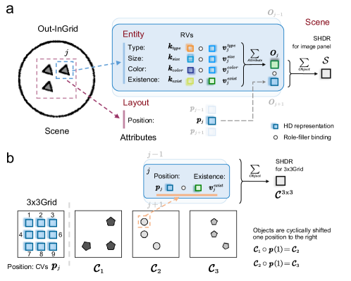
Figure 3: Structured HD representations (SHDR) for the image panel and the nxn Grid. (a) SHDR for the image panel (Equation 10). Taking the Out-InGrid configuration as an example, an image panel contains multiple objects, each with four entity attributes: type, size, color, and existence. Through the first layer of role-filler binding, these attributes are combined to form a SHDR for each object. Additionally, at the layout level, each object has a position attribute. By applying a second layer of role-filler binding, the SHDR for the entire image panel is constructed. (b) SHDR for the nxn Grid (Equation 12). Taking the 3x3Grid configuration as an example, the position vectors for all objects are represented using circular vectors (CVs) with a period of $3\times 3=9$. The SHDR $\mathcal{C}^{3\mathrm{x}3}$ for this 3x3Grid is obtained by performing role-filler binding between the corresponding position vectors $\boldsymbol{p}_{j}$ and existence vectors $\boldsymbol{v}_{j}$. Due to the periodic nature of the position vectors, as all objects shift positions cyclically, the SHDR undergoes a binding operation with the position vectors corresponding to the magnitude of the shift.

IV-B2 Inverse relation functions

Rule execution in RPM requires inferring the third attribute value based on the first two attribute values in a row of panels, given a known relation. It represents an inverse problem of rule abduction. In the vector-symbolic method, given the operator power ${OP_{1:M}}$ and the output $\boldsymbol{r}$, the last vector representation $\boldsymbol{v}_{N}$ can be inferred from the first $N-1$ inputs $\boldsymbol{v}_{1:N-1}$ using the inverse of the relation functions (Figure 2g). According to Equation 6, the inverse numerical relation function is defined as follows:

$$\boldsymbol{v}_{N} =R_{Num}^{-1}\left(\boldsymbol{v}_{1:N-1},OP_{1:M},\boldsymbol{r}\right)$$ (8)

$$=\left(\circ_{i=1}^{N-1}\boldsymbol{v}_{i}^{\left(\circ\left(-op_{i}/op_{M}\right)\right)}\right)\circ\boldsymbol{r}^{\left(\circ\left(-1/op_{M}\right)\right)}$$

Similarly, according to Equation 7, the inverse logical relation function is defined as follows:

$$\boldsymbol{v}_{N} =R_{Lgc}^{-1}\left(\boldsymbol{v}_{1:N-1},OP_{1:M},\boldsymbol{r}\right)$$ (9)

$$=op_{3}\left(op_{1}\boldsymbol{v}_{1}\land op_{2}\boldsymbol{v}_{2}\right)$$

.

IV-C Structured high-dimensional representation and its attribution decomposition

VSA can create structured symbolic representations using atomic HD vector representations and decouple them directly from these structures through algebraic operations [hersche2023neuro]. This subsection presents the process of constructing a structured HD representation (SHDR) for an image panel and its decomposition to retrieve individual attribute representations. Additionally, an SHDR for the nxn Grid ($n=2,3$) at the component level is also introduced.

IV-C1 SHDR for the image panel

In RAVEN dataset, each image panel consists of objects, with each object characterized by multiple attributes. Consequently, the structured HD representation (SHDR) for each image panel can be obtained through two layers of role-filler bindings (Figure 3a). First, the bundling operation is used to construct an SHDR for each object at the entity level by combining its attributes. Then, another bundling operation aggregates these object-level representations to construct a SHDR of the image panel at the scene level. Therefore, each image panel $\mathcal{X}\in\mathbb{R}^{r\times r}$, with a resolution $r\times r$, can be represented by an SHDR $\mathcal{S}\in\mathbb{R}^{d}$ as follows:

$$\mathcal{S} =\sum_{j=1}^{N_{pos}}{\boldsymbol{p}_{j}\circ\boldsymbol{O}_{j}}$$ (10)

$$=\sum_{j=1}^{N_{pos}}{\boldsymbol{p}_{j}\circ\left(\sum_{attr\in ATTR}{\boldsymbol{k}_{attr}\circ\boldsymbol{v}_{j}^{attr}}\right)}$$

Here, $\boldsymbol{O}_{j}$ represents the SHDR of the $j$th object with different attributes at the entity level, incorporating attributes such as type, size, color, and existence. The attribute set is $ATTR=\left\{type,size,color,exist\right\}$. At the entity level, the key vector $\boldsymbol{k}_{attr}$ denotes the class of a specific attribute $attr\in ATTR$, while the value vector $\boldsymbol{v}_{j}^{attr}$ indicates the attribute’s value at the position $j$. At the scene level, the position vector $\boldsymbol{p}_{j}$ specifies the location of the $j$-th object.

IV-C2 Representation decomposition

Given an estimated SHDR $\hat{\mathcal{S}}\in\mathbb{R}^{d}$ of an image panel, all SHDRs of objects $\hat{\boldsymbol{O}}_{j}$ at the entity level, along with the corresponding attribute representations $\hat{\boldsymbol{v}}_{j}^{attr}$, can be derived through a series of unbinding operations [kleyko2022survey]. The decomposition process is shown as follows:

$$\begin{cases}\hat{\boldsymbol{O}}_{j}=\boldsymbol{p}_{j}\oslash\hat{\mathcal{S}}=\boldsymbol{p}_{l}^{-1}\circ\hat{\mathcal{S}}\\ \hat{\boldsymbol{v}}_{j}^{attr}=\boldsymbol{k}_{attr}\oslash\hat{\boldsymbol{O}}_{j}=\boldsymbol{k}_{attr}^{-1}\circ\hat{\boldsymbol{O}}_{j}\\ \end{cases}$$ (11)

It is important to note that due to inaccuracies in the estimated SHDR $\hat{\mathcal{S}}$ and the noise introduced by the unbinding operation, the estimated attribute representations $\hat{\boldsymbol{v}}_{j}^{attr}$ may not fully match the original $\boldsymbol{v}_{j}^{attr}$ used in Equation 10.

IV-C3 SHDR for the nxn Grid component

In the RAVEN dataset, three figure configurations—2x2Grid, 3x3Grid, and Out-InGrid—include components where objects are arranged in an nxn grid pattern at the layout level [zhang2019raven]. Since the positions in the nxn Grid involve component-level rule reasoning, the SHDR for the nxn Grid component ($n=2,3$), focusing only on positions and object existence, is introduced as follows (Figure 3b):

$$\mathcal{C}^{\mathrm{nxn}}=\sum_{j=1}^{n\times n}{\boldsymbol{p}_{j}\circ\boldsymbol{v}_{j}^{exist}}$$ (12)

IV-D Rules from the perspective of relation functions

TABLE III: Attribute representations and the relation functions involved in rule abductions