Incorporating stochastic gene expression, signaling-mediated intercellular interactions, and regulated cell proliferation in models of coordinated tissue development

Abstract

Formulating quantitative and predictive models for tissue development requires consideration of the complex, stochastic gene expression dynamics, its regulation via cell-to-cell interactions, and cell proliferation. Including all of these processes into a practical mathematical framework requires complex expressions that are difficult to interpret and apply. We construct a simple theory that incorporates intracellular stochastic gene expression dynamics, signaling chemicals that influence these dynamics and mediate cell-cell interactions, and cell proliferation and its accompanying differentiation. Cellular states (genetic and epigenetic) are described by a Waddington vector field that allows for non-gradient dynamics (cycles, entropy production, loss of detailed balance) which is precluded in Waddington potential landscape representations of gene expression dynamics. We define an epigenetic fitness landscape that describes the proliferation of different cell types, and elucidate how this fitness landscape is related to Waddington’s vector field. We illustrate the applicability of our framework by analyzing two model systems: an interacting two-gene differentiation process and a spatiotemporal organism model inspired by planaria.

I Introduction

Cell and tissue development is a complex and multifaceted dynamical process, involving gene regulatory dynamics, cell-to-cell interactions, and differential cell proliferation and death rates. The conceptual model of Waddington’s landscape has been a guiding paradigm for understanding the mechanisms of cell development [1, 2, 3]. Waddington’s landscape suggests that the internal dynamics of a differentiating cell follow that of a particle in a rugged high-dimensional “potential” landscape. However, the internal dynamics of cell states (e.g., gene expression profiles) are only one aspect of tissue development. Proliferation and death of individual cells give rise to population dynamics akin to that seen under Darwinian evolution [4, 5]. Additionally, intracell gene dynamics and population-level birth-death processes are coupled through cell-to-cell signaling and metabolic interactions [5, 6]. Thus, a complete description of development must describe an interacting population of cells, not just the gene dynamics within a single cell.

The conceptual framework of Waddington’s landscape has been translated into a variety of mathematical models. For example, Waddington’s landscape has been interpreted as a potential landscape acting on single-cell gene expression [7, 3, 8, 9, 10, 11, 6] and on population level phenotypes [12]. In the typical single-cell interpretation, a cell’s state is modeled as a particle with position ${\bm{x}}$ in a potential energy landscape $U({\bm{x}})$ in a noisy environment. This model implies that one can reconstruct $U({\bm{x}})$ from data using the simple relationship $U({\bm{x}})=-\log p_{\rm ss}({\bm{x}})$, where $p_{\rm ss}({\bm{x}})$ is the steady-state distribution of states empirically measured. Such formulae have been applied to real datasets [13] but its use is hampered by its inherent limitation to a single cell (or to non-interacting and non-proliferating populations) and the assumption of both gradient dynamics and dynamics that obey detailed balance among gene regulation states.

When cell division and death are considered, the concept of a fitness landscape becomes relevant. In evolutionary population dynamics, high fitness genotypes elicit high proliferation rates; this concept must be adapted to the context of development, where all cells have the same genotype. Mathematical models of development often consider a single-cell fates and state changes [14, 13, 15, 8, 3, 16, 17, 18, 19, 20, 21, 22]; those that incorporate cell population dynamics through birth and death typically neglect cell-cell interactions [23, 24, 25, 26, 27, 28]. In kinetic theories that combine internal cell state dynamics with state-dependent division and death rates, tractable dynamical equations describing population-level quantities can be derived if there are no cell-cell interactions [29, 30, 31, 32]. However, in developing tissue, cell division and death are tightly coordinated through cell-cell interactions mediated by secreted chemical signals that influence gene expression in other cells [33, 34]. Failure of this regulated tissue development can lead to pathologies such as cancer [35, 36]. Thus, effective theoretical approaches that incorporate regulated intracell gene expression with population-level birth-death processes will provide critical tools for modeling and analyzing tissue development and evolution.

In this paper, we present a general framework for modeling a general developmental process in which cell-cell interactions regulate gene expression and cell proliferation. Our framework describes a population of individual (discrete) cells, rather than assuming an infinite continuum of cells, as has been done in other works [26, 25, 5, 6]. In the tissue development context, our framework also includes spatial structure, enabling models of coordinated tissue development in which a small initial population of stem cells robustly develops into a stable and self-healing tissue. Our approach incorporates all known important processes in an interpretable way, allowing us to better define the concepts of the Waddington landscape and fitness landscape in the context of development. Rather than use a Waddington landscape that assumes gradient dynamics, we use a Waddington vector field to account for non-gradient dynamics of gene expression. Such detailed-balance-violating stochastic dynamics is expected in an energy-consuming process such as cell state regulation and homeostasis.

We also define an effective epigenetic fitness landscape. Whereas a fitness landscape describes differential proliferation of different genotypes, our epigenetic fitness landscape describes the differential proliferation of cells of the same genotype type but differing epigenetic state, capturing the fact that different attractors of the gene regulatory dynamics induce different cell division and death rates. In addition, we show how our general model can be reduced to simpler forms by applying common assumptions. Often, such assumptions are implicitly included in models of development, leading to confusion regarding the realm of applicability of such models. Our general framework provides a starting point for deriving simpler, interpretable models by applying explicitly-stated assumptions. We present two models of the robust development of a stable tissue population as proof-of-concept examples. The first is a well-mixed model of gene-regulated stem cell differentiation, and the second is a spatiotemporal model of a regenerating organism, similar to planaria.

II Mathematical Framework

Here, we assemble all the relevant physical processes that are understood to play roles in a developing tissue. The dependencies (and feedback) across scales and among these mechanisms are clearly delineated by proper definitions and judicious approximations/assumptions.

II.1 Intracellular state dynamics

Let ${\bm{z}}\in\mathbb{R}^{d_{z}}$ denote the internal state of a cell. ${\bm{z}}$ specifies the state of the relevant gene regulatory network(s) in the cell, and, in principle, could also specify the methylation of DNA, chromatin structure, spatial organization of organelles, and/or any other relevant variables. While a complete specification of the gene regulatory network state requires specification of both protein and mRNA concentrations within the cell, the relatively fast timescales of mRNA transcription and degradation compared to protein translation and degradation can justify a quasi-steady state approximation where only protein concentrations need be specified. We label cells by a superscript $\alpha$, i.e., ${\bm{z}}^{\alpha}$ is the state of cell $\alpha$, where $\alpha=1,...,N(t)$, and $N(t)$ is the total number of cells which varies from cell division and death .

To allow for spatial resolution, let $\bm{r}^{\alpha}\in\mathbb{R}^{3}$ denote cell $\alpha$’s position in 3-dimensional space. Interactions between cells are typically mediated by signaling molecules; suppose there are $L$ relevant signaling molecules and let $c_{\ell}(\bm{r},t)$ denote the concentration of signaling molecule $\ell$ ($\ell=1,...,L$) at position $\bm{r}$ at time $t$. For notational convenience, let ${\bm{c}}(\bm{r},t)=(c_{1}(\bm{r},t),...,c_{L}(\bm{r},t))$ denote the list of signaling molecule concentrations. For cell $\alpha$ at position $\bm{r}^{\alpha}$, the dynamics of its state ${\bm{z}}^{\alpha}(t)$ are modeled by a stochastic differential equation (SDE):

$$\mbox{d}{\bm{z}}^{\alpha}=\bm{F}({\bm{z}}^{\alpha};{\bm{c}}^{\alpha})\mbox{d}t+\sigma({\bm{z}}^{\alpha};{\bm{c}}^{\alpha})\mbox{d}\bm{B}^{\alpha},$$ (1)

where ${\bm{c}}^{\alpha}\equiv{\bm{c}}(\bm{r}^{\alpha},t)$ are the signaling concentrations experienced by cell $\alpha$ at time $t$. $\bm{F}({\bm{z}};{\bm{c}})$ defines a ${\bm{c}}$-dependent vector field that maps $\mathbb{R}^{d_{z}}\to\mathbb{R}^{d_{z}}$ and which describes the deterministic component of the cell state dynamics. We call $\bm{F}({\bm{z}};{\bm{c}})$ Waddington’s vector field, and it is presumed to have stable attractors corresponding to stable cell types. Importantly, the signaling molecule concentration ${\bm{c}}^{\alpha}$ influences the dynamics of the state ${\bm{z}}^{\alpha}$, and the dynamics of ${\bm{c}}(\bm{r},t)$ are governed by the states and positions of all cells (as described below). Hence, the signaling molecules can mediate cell-to-cell interactions, allowing the tissue to develop in a coordinated way. In the special case that $\bm{F}({\bm{z}};{\bm{c}})$ is the negative gradient of a function, $\bm{F}({\bm{z}};{\bm{c}})=-\nabla_{\bm{z}}U({\bm{z}};{\bm{c}})$, then $U({\bm{z}};{\bm{c}})$ would be the traditional Waddington landscape. However, we do not assume that $\bm{F}({\bm{z}};{\bm{c}})$ is the gradient of any function, and in section IV we review and discuss the limitations of the traditional Waddington landscape picture. Noise is characterized by the $d_{b}$-dimensional Brownian noise $\mbox{d}\bm{B}^{\alpha}$ and by the amplitude $\sigma({\bm{z}};{\bm{c}})$, a $d_{z}\times d_{b}$ matrix which may depend on the cell state and signaling molecule concentrations that the cell experiences.

II.2 Cell-cell interactions through signaling molecules

The dynamics of signaling molecule concentrations can be modeled by any variety of molecular transport models. For example, a deterministic PDE describing excretion, absorption, and diffusion of signaling molecules takes on the typical form [38]

$$\partial_{t}c_{\ell}(\bm{r},t)=D_{\ell}\nabla^{2}c_{\ell}-d_{\ell}c_{\ell}+\sum_{\text{cells }\alpha}\!\!\lambda_{\ell}(\bm{r}-\bm{r}^{\alpha}\!,{\bm{z}}^{\alpha}),$$ (2)

where $\lambda_{\ell}(\bm{r}-\bm{r}^{\alpha}\!,{\bm{z}}^{\alpha})$ is the excretion rate of signaling molecule $\ell$ at position $\bm{r}$ from a cell in state ${\bm{z}}^{\alpha}$ centered at $\bm{r}^{\alpha}$, and the sum runs over all cells. The function $\lambda_{\ell}(\bm{r}-\bm{r}^{\alpha}\!,{\bm{z}}^{\alpha})$ is localized about $\bm{r}^{\alpha}$ and represents the spatial extent of a cell that exports signaling molecule. Diffusion and degradation of molecule $\ell$ is described by the coefficients $D_{\ell}$ and $d_{\ell}$, respectively. A natural choice of boundary condition for Eq. 2 is $c_{\ell}(\bm{r})\to 0$ as $|\bm{r}|\to\infty$. Alternatively, to model in subcompartments or spatially defined microenvironments, Eq. 2 can be considered in finite regions of space each with appropriate boundary conditions. For a closed environment, one would use reflecting boundary conditions for $c_{\ell}(\bm{r})$. Eq. 2 neglects reactions amongst the signaling molecules and models deterministic or locally averaged concentrations, appropriate for molecular transport at high concentrations and/or fast molecular timescales. At very low signaling molecule densities, intrinsic molecular stochasticity may be important and any number of stochastic models [39, 40, 41] and simulation approaches [42, 43] are available. Fig. 1 provides a schematic of signaling-molecule-mediated interactions among cells at positions $\bm{r}^{\alpha}$, with potentially different internal states ${\bm{z}}^{\alpha}$.

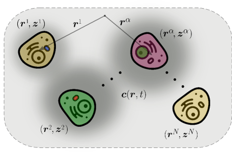
Figure 1: Schematic of cells at various positions $\bm{r}^{\alpha}$ and in various gene expression states ${\bm{z}}^{\alpha},\,\alpha=1,2,...,N$. Cell-cell interactions mediated by position-dependent signaling molecule concentrations ${\bm{c}}(\bm{r},t)\equiv\big{(}c_{1}(\bm{r},t),...,c_{L}(\bm{r},t)\big{)}$ which are represented in gray-scale. Cells can produce signaling molecules at rates that depend on ${\bm{z}}$; gene expression is in turn influenced by the concentrations that a cell senses, leading to potentially complex cell-cell interactions.

II.3 Cell migration

Cells may also migrate by exerting forces on neighboring cells or on their substrate; this migration may be influenced by signaling molecules (chemokines). Such coordinated movement is essential for tissue development [44, 45]. One can straightforwardly couple molecular signaling with cell motion [46], and a general stochastic model for cell motion can be expressed using an SDE such as

$$\mbox{d}\bm{r}^{\alpha}(t)=\bm{g}(\bm{r}^{\alpha},S(t))\mbox{d}t+\eta(\bm{r}^{\alpha},S(t))\mbox{d}\bm{W}^{\alpha}$$ (3)

where $S(t)=\{(\bm{r}^{\alpha}(t),{\bm{z}}^{\alpha}(t))\}_{\alpha=1}^{N(t)}$ is the full state of the tissue population and $\mbox{d}\bm{W}^{\alpha}$ is a 3-dimensional Brownian noise. The mean velocity $\bm{g}$ and noise amplitude $\eta$ (a $3\times 3$ matrix) can depend on the cell’s position $\bm{r}^{\alpha}$ as well as on the full state of the tissue $S(t)$. Although explicit dependence of $\bm{g}$ and $\eta$ on the spatial profile of signaling molecule concentrations is not included in Eq. 3, one could consider a velocity $\bm{g}$ which depends on $\nabla{\bm{c}}(\bm{r}^{\alpha},t)$, or on higher derivatives of the concentration profile. Eq. 3 is a Langevin equation for fluctuating cell positions. Many related models for cell motion, including anomalous diffusion and longer-ranged hopping have been developed [47, 48, 49].

II.4 Cell proliferation (and death)

During cell division—a process involving cellular-scale disruption and reorganization—a mother cell divides into two daughter cells which may acquire states that are different from the state of the mother. In our model, cells have a state-dependent and concentration-dependent division rate, denoted $\beta({\bm{z}};{\bm{c}})$ for a cell in state ${\bm{z}}$ and with signaling molecule concentrations ${\bm{c}}$ at its location (to be precise, cell $\alpha$ has division rate $\beta({\bm{z}}^{\alpha};{\bm{c}}^{\alpha})$, but we will drop the superscript $\alpha$ to avoid cumbersome notation). $\beta({\bm{z}};{\bm{c}})$ is a marginal probability over the joint distribution for the probability of a cell in state ${\bm{z}}$ dividing into daughters with states ${\bm{z}}^{\prime}$, ${\bm{z}}^{\prime\prime}$ and with positional displacements from the mother $\Delta\bm{r}^{\prime}$, $\Delta\bm{r}^{\prime\prime}$. This joint distribution is denoted as

$$\tilde{\beta}\big{(}{\bm{z}};{\bm{c}};{\bm{z}}^{\prime},{\bm{z}}^{\prime\prime},\Delta\bm{r}^{\prime},\Delta\bm{r}^{\prime\prime}\big{)}$$ (4)

and is invariant under exchange of ${\bm{z}}^{\prime}$ and ${\bm{z}}^{\prime\prime}$ and under exchange of $\Delta\bm{r}^{\prime}$ and $\Delta\bm{r}^{\prime\prime}$. Marginalizing, we find the overall division rate

$$\beta({\bm{z}};{\bm{c}})=\int\!\tilde{\beta}\big{(}{\bm{z}};{\bm{c}};{\bm{z}}^{\prime},{\bm{z}}^{\prime\prime}\!,\Delta\bm{r}^{\prime},\Delta\bm{r}^{\prime\prime}\big{)}\mbox{d}{\bm{z}}^{\prime}\mbox{d}{\bm{z}}^{\prime\prime}\mbox{d}\Delta\bm{r}^{\prime}\mbox{d}\Delta\bm{r}^{\prime\prime}.$$ (5)

Finally, cell death occurs at rate $\mu({\bm{z}};{\bm{c}})$, which can depend on both ${\bm{z}}$ and ${\bm{c}}$.

Eqs. 1, 2, and 3, along with system-specific models for birth and death rates, $\tilde{\beta}({\bm{z}};{\bm{c}};{\bm{z}}^{\prime},{\bm{z}}^{\prime\prime},\Delta\bm{r}^{\prime},\Delta\bm{r}^{\prime\prime})$ and $\mu({\bm{z}};{\bm{c}})$, form our general description of developing cell populations. The following section illustrates how common assumptions can be incorporated to significantly simplify the model.

III Simplifying assumptions

Here we describe a series of assumptions that can be applied to further simplify our mathematical model. Our examples in Sections V and VI show how various combinations of these assumption can be used to obtain models that capture different degrees of detail.

III.1 Fast equilibration of signaling molecule concentrations

Suppose the concentrations $c_{\ell}(\bm{r},t)$ reach steady state on timescales shorter than those associated with gene expression dynamics, cell movement, and cell division and death. We can approximate $c_{\ell}(\bm{r},t)$ by the quasi-steady state solution of Eq. 2 under the instantaneous state of the population $S(t)=\{{\bm{z}}^{\alpha}(t),\bm{r}^{\alpha}(t)\}_{\alpha=1}^{N(t)}$. We denote this quasi-steady state concentration profile by $c^{\rm ss}_{\ell}(\bm{r};S(t))$. For signaling molecule dynamics described by Eq. 2, $c^{\rm ss}_{\ell}(\bm{r};S(t))$ takes the explicit form

$$c^{\rm ss}_{\ell}\big{(}\bm{r};S(t)\big{)}=\sum_{\text{cells }\alpha}c^{(1)}_{\ell}(\bm{r}-\bm{r}^{\alpha},{\bm{z}}^{\alpha})$$ (6)

where $c^{(1)}_{\ell}(\bm{r},{\bm{z}})$ is the concentration profile produced by a single isolated cell at position $\bm{r}=\bm{0}$, given by the solution to

$$0=D_{\ell}\nabla_{\bm{r}}^{2}c^{(1)}_{\ell}(\bm{r},{\bm{z}})-d_{\ell}c^{(1)}_{\ell}(\bm{r},{\bm{z}})+\lambda_{\ell}(\bm{r},{\bm{z}})$$ (7)

with appropriate boundary conditions.

III.2 Well-mixed population

In a further approximation, that may apply to e.g., well-mixed populations of stem cells that differentiate in microenvironments, spatial distributions of cells and signaling molecules can both be treated as spatially averaged quantities. Hence, Eq. 3 can be ignored and $c_{\ell}$ is independent of $\bm{r}$. If the dynamics of $c_{\ell}$ are given by Eq. 2 with reflecting boundary conditions, then Eq. 2 can be replaced by an ODE for the mean concentration $\bar{c}(t)=(1/V)\int c_{\ell}(\bm{r})\mbox{d}\bm{r}$ over the closed volume $V$

$$\frac{\mbox{d}\bar{c}_{\ell}}{\mbox{d}t}=\sum_{\text{cells }\alpha}\bar{\lambda}_{\ell}({\bm{z}}^{\alpha})-d_{\ell}\bar{c}_{\ell}$$ (8)

where $\bar{\lambda}_{\ell}({\bm{z}})=(1/V)\int\lambda_{\ell}(\bm{r},{\bm{z}})\mbox{d}\bm{r}$ is the spatially averaged excretion rate of each of the uniformly distributed cells. If signaling molecules reach steady state rapidly, then the signaling molecule concentrations are

$$c^{\rm ss}_{\ell}=\frac{1}{d_{\ell}}\sum_{\text{cells }\alpha}\bar{\lambda}_{\ell}({\bm{z}}^{\alpha}).$$ (9)

III.3 Fast ${\bm{z}}$ dynamics and discrete cell types

For fast cell state dynamics, the state ${\bm{z}}^{\alpha}$ of cell $\alpha$ rapidly reaches an attractor of $\bm{F}({\bm{z}}^{\alpha};{\bm{c}}^{\alpha})$ but can make stochastic transitions to different attractors. Hence, we can approximate the continuous state space by the discrete set of attractors, labeled $q=1,...,Q$. Such a discrete approximation of an otherwise continuous or highly granular set of cell states has been shown to be useful in many developmental contexts such as embryonic stem cell differentiation [50, 21, 22]. The Waddington vector field $\bm{F}({\bm{z}}^{\alpha};{\bm{c}}^{\alpha})$ is then replaced by a matrix of jump rates, $F_{q,q^{\prime}}({\bm{c}}^{\alpha})$, specifying the jump rate from $q$ to $q^{\prime}$. These jump rates can, in principle, be estimated numerically via simulations of Eq. 1. Alternatively, if $\bm{F}({\bm{z}}^{\alpha};{\bm{c}}^{\alpha})$ is the gradient of a Waddington landscape, then Kramers’ rate formula can be used to approximate the jump rates [51].

The division rate at which cell $\alpha$ in attractor $q$ divides into daughter cells at attractor states $q^{\prime},q^{\prime\prime}$ with positional displacements $\Delta\bm{r}^{\prime},\Delta\bm{r}^{\prime\prime}$ is denoted $\tilde{\beta}_{q,q^{\prime},q^{\prime\prime}}({\bm{c}};\Delta\bm{r}^{\prime},\Delta\bm{r}^{\prime\prime})$. Just as for Eq. 4, $\tilde{\beta}_{q,q^{\prime},q^{\prime\prime}}({\bm{c}};\Delta\bm{r}^{\prime},\Delta\bm{r}^{\prime\prime})$ is invariant under exchange of $q^{\prime}$ and $q^{\prime\prime}$, as well as under exchange of $\Delta\bm{r}^{\prime}$ and $\Delta\bm{r}^{\prime\prime}$. The diagonal elements $\tilde{\beta}_{q,q,q}$ correspond to symmetric division in which both daughters have the same state as the mother, whereas elements with $q^{\prime}\neq q^{\prime\prime}$ correspond to asymmetric division. Letting ${\bm{z}}_{q}$ denote the attractor state $q$, these division rates are given by $\tilde{\beta}_{q,q^{\prime},q^{\prime\prime}}({\bm{c}};\Delta\bm{r}^{\prime},\Delta\bm{r}^{\prime\prime})=\tilde{\beta}({\bm{z}}_{q};{\bm{c}};{\bm{z}}_{q^{\prime}},{\bm{z}}_{q^{\prime\prime}},\Delta\bm{r}^{\prime},\Delta\bm{r}^{\prime\prime})$. The death rate in attractor $q$ is $\mu_{q}(c)=\mu({\bm{z}}_{q};{\bm{c}})$.

III.4 Unifying the assumptions

If all three of the above simplifying approximations (fast equilibration of signaling molecules, well-mixed population, and discrete cell types) hold, our model simplifies significantly. Let the vector ${\bf n}\equiv(n_{1},...,n_{Q})$ specify the cell populations in the tissue, where $n_{q}$ is the number of cells of type $q$. Let $\beta_{q,q^{\prime},q^{\prime\prime}}({\bm{c}})\equiv\int\tilde{\beta}_{q,q^{\prime},q^{\prime\prime}}({\bm{c}};\Delta\bm{r}^{\prime},\Delta\bm{r}^{\prime\prime})\mbox{d}\Delta\bm{r}^{\prime}\mbox{d}\Delta\bm{r}^{\prime\prime}$ be the division rate of a mother of type $q$ into daughters of type $q^{\prime},q^{\prime\prime}$. Signaling concentrations ${\bm{c}}({\bf n})$ are functions of only ${\bf n}$, and are determined by Eq. 9.

The probability $P({\bf n},t)$ of having a tissue state ${\bf n}$ at time $t$ evolves accord to the following master equation:

$$\partial_{t}P({\bf n},t)= \sum_{q,q^{\prime},q^{\prime\prime}}\Big{[}(n_{q}+1)\beta_{q,q^{\prime},q^{\prime\prime}}\big{(}{\bm{c}}({\bf n}_{q+,q^{\prime}-,q^{\prime\prime}-})\big{)}P({\bf n}_{q+,q^{\prime}-,q^{\prime\prime}-})-n_{q}\beta_{q,q^{\prime},q^{\prime\prime}}\big{(}{\bm{c}}({\bf n})\big{)}P({\bf n})\Big{]}$$ (10)

$$+\sum_{q,q^{\prime}}\Big{[}(n_{q}+1)F_{q,q^{\prime}}\big{(}{\bm{c}}({\bf n}_{q+,q^{\prime}-})\big{)}P({\bf n}_{q+,q^{\prime}-})-n_{q}F_{q,q^{\prime}}\big{(}{\bm{c}}({\bf n})\big{)}P({\bf n})\Big{]}$$

$$+\sum_{q}\Big{[}(n_{q}+1)\mu_{q}\big{(}{\bm{c}}({\bf n}_{q+})\big{)}P({\bf n}_{q+})-n_{q}\mu_{q}\big{(}{\bm{c}}({\bf n})\big{)}P({\bf n})\Big{]}$$

In analogy with the bookkeeping notation used in [29, 30], ${\bf n}_{q+,q^{\prime}-,q^{\prime\prime}-}$ denotes a system state with, compared to system state ${\bf n}$, one more type $q$ cell and one fewer cell of type $q^{\prime}$ and one fewer cell of type $q^{\prime\prime}$. Hence, ${\bf n}_{q+,q^{\prime}-,q^{\prime\prime}-}$ is the system state that converts into state ${\bf n}$ when a mother cell of type $q$ divides into daughter cells of type $q^{\prime}$ and $q^{\prime\prime}$. Similarly, ${\bf n}_{q+,q^{\prime}-}$ denotes a system state with one more type $q$ cell and one fewer type $q^{\prime}$ cell relative to system state ${\bf n}$. ${\bf n}_{q+}$ denotes a system state with one more type $q$ cell than in system state ${\bf n}$. Equation 10 represents a master equation for the probability density for populations of cells of multiple types and is a simpler form of master equations studied in [52, 29, 30]. For small populations and few accessible cell types, solving this linear master equation or simulating the process is computationally feasible.

III.5 Developmental Fitness landscape

Proliferation of certain cell types over others due to differing division and death rates is a crucial aspect of development. Differential proliferation is also key to evolutionary dynamics, where genotypes that induce high net growth rates eventually comprise larger portions of the overall population. In evolutionary dynamics, preferential growth is described by a fitness landscape, typically defined as a function which specifies the net growth (division minus death) rate $\phi_{g}$ of a cell or organism given its genotype $g$. Here, we adapt this concept to the context of cell development to define an epigenetic fitness landscape which specifies which cell types proliferate in the developing tissue.

A key difference between evolutionary dynamics (or speciation) and development is that, in a developing tissue, all cells have the same genotype (aside from rare mutations) and differences in cells’ division rates are due to differences in their cell type, determined by the internal state ${\bm{z}}$. We define the developmental fitness of cell type $q$, denoted $\phi_{q}({\bf n})$, as the net proliferation rate of type $q$ cells, absent production of type $q$ cells through division of other cell types or stochastic jumps from other cell types. $\phi_{q}({\bf n})$ depends on the tissue population state ${\bf n}$ due to cell-cell interactions via signaling molecules. In defining $\phi_{q}({\bf n})$, we adopt the assumptions from the previous sections, namely, fast equilibration of signaling molecules, well-mixed population, and discrete cell types. Within our framework, we can define fitness mathematically as

$$\phi_{q}({\bf n})= \beta_{q,q,q}\big{(}{\bm{c}}({\bf n})\big{)}-\beta_{q,\rm lost}\big{(}{\bm{c}}({\bf n})\big{)}$$ (11)

$$\qquad\quad-F_{q,\rm lost}\big{(}{\bm{c}}({\bf n})\big{)}-\mu_{q}\big{(}{\bm{c}}({\bf n})\big{)}$$

where $\beta_{q,q,q}({\bm{c}})$ is the rate of symmetric division in which a mother cell of type $q$ divides into two daughter cells of type $q$. $\beta_{q,\text{lost}}({\bm{c}})\equiv\sum_{q^{\prime}\neq q,q^{\prime\prime}\neq q}\beta_{q,q^{\prime},q^{\prime\prime}}({\bm{c}})$ is the rate at which a mother cell of type $q$ divides into daughter cells, both of whose cell types differ from that of the mother cell. Note that asymmetric division, where a cell of type $q$ divides into daughters of type $q$ and $q^{\prime}\neq q$, leaves the population of type $q$ cells unchanged, and therefore does not factor into the developmental fitness landscape. $F_{q,\text{lost}}({\bm{c}})=\sum_{q^{\prime}\neq q}F_{q,q^{\prime}}({\bm{c}})$ is the jump rate of type $q$ cells to a different type.

The following subsection shows how, in the limit of large tissue size, the developmental fitness landscape contributes to tissue dynamics through a simple equation.

III.6 Deterministic limit

In the limit of large tissue size, Eq. 10 predicts that cell densities in the tissue follow deterministic dynamics. This limit is analogous to how deterministic mass action equations (ODEs) emerge from a more microscopic chemical master equation description in the limit of large system size. Recall that Eq. 10 describes the population within a region of fixed volume, and denote this volume by $V_{0}$. Then, $\bm{\rho}\equiv{\bf n}/V_{0}$ are the cell type densities in the tissue described by Eq. 10. Now, consider a system with volume $V>V_{0}$ and take the limit that $V\to\infty$ while $\bm{\rho}$ remains fixed. The mass-action dynamics in this limit are described by

$$\frac{\mbox{d}\bm{\rho}}{\mbox{d}t}=\text{diag}(\bm{\phi}(\bm{\rho}V_{0}))\bm{\rho}+\bm{m}(\bm{\rho}V_{0})\bm{\rho}$$ (12)

where $\bm{\phi}({\bf n})=(\phi_{1}({\bf n}),...,\phi_{Q}({\bf n}))$ is the developmental fitness landscape defined in the previous section, and $\text{diag}(\bm{\phi}(\bm{\rho}V_{0}))$ denotes the $Q\times Q$ matrix with the elements of $\bm{\phi}(\bm{\rho}V_{0})$ on the diagonal. $\bm{m}(\bm{\rho}V_{0})$ is a zero-diagonal matrix which contains the jump rates and asymmetric division rates through which cells of one type produce cells of another type. The matrix elements are explicitly

$$m_{q,q^{\prime}}({\bf n})= F_{q^{\prime},q}\big{(}{\bm{c}}({\bf n})\big{)}+2\beta_{q^{\prime},q,q}\big{(}{\bm{c}}({\bf n})\big{)}$$ (13)

$$\qquad\qquad+2\!\sum_{q^{\prime\prime}\neq q}\beta_{q^{\prime},q,q^{\prime\prime}}\big{(}{\bm{c}}({\bf n})\big{)}.$$

The factor of 2 in the third term arises from the symmetry of $\beta_{q^{\prime},q,^{\prime\prime}}$ with respect to exchange of the final two indices.

Deterministic dynamical models of interacting population dynamics, as could be described by Eq. 12, have been used to model aspects of development [53]. Note that the stochastic fluctuations in the dynamics of $\bm{\rho}$ are proportional to $(V/V_{0})^{-1/2}$, which vanishes as $V\to\infty$. For large but finite $V$, the stochastic component of the dynamics can be obtained with the van Kampen system size expansion [54].

IV Waddington’s Landscape vs Waddington’s vector field

From among the various interpretations of Waddington’s landscape that have been studied. The most common interpretation that has emerged is that the vector field $\bm{F}({\bm{z}};{\bm{c}})$ in Eq. 1 is a negative gradient of a function $U({\bm{z}};{\bm{c}})$,

$$\bm{F}({\bm{z}};{\bm{c}})=-\nabla_{{\bm{z}}}U({\bm{z}};{\bm{c}}),$$ (14)

where $U({\bm{z}};{\bm{c}})$ is called a Waddington landscape [3, 25, 23, 9]. We call a stochastic dynamical system of this form, where the deterministic part is the negative gradient of a potential landscape, a gradient system. If the noise in Eq. 1 is additive (meaning $\sigma$ is independent of ${\bm{z}}$), then $U({\bm{z}};{\bm{c}})$ can be reconstructed from experimental measurement of the steady state distribution of cell states at fixed signaling molecule concentrations, $p_{\rm ss}({\bm{z}};{\bm{c}})$, via [3]

$$U({\bm{z}};{\bm{c}})=-\log p_{\text{ss}}({\bm{z}};{\bm{c}}).$$ (15)

The validity and generality of this Waddington landscape framework has been a topic of considerable discussion and disagreement. On one hand, it has been pointed out that realistic dynamics of protein and mRNA concentrations are not gradient systems, but rather have curl (or the higher-dimensional generalization of curl) [14, 16, 28]. On the other hand, it has been noted that for nearly all vector fields $\bm{F}$ without limit cycles (specifically, for Morse-Smale systems), the vector field $\bm{F}$ can be converted to the negative gradient of a potential landscape with a coordinate transformation [8]. Hence, a very broad class of models, including most models of protein and mRNA dynamics, can be expressed as gradient systems under a suitable choice of coordinates. This suggests that the Waddington landscape picture is highly general.

However, noise has a crucial effect which significantly hinders the generality of the landscape picture. Eq. 15 is valid only for additive noise, yet the noise in the dynamics of protein and mRNA concentrations is typically non-additive [9]. It was recently demonstrated how the mis-application of Eq. 15 to systems with non-additive noise can ‘add’ or ‘delete’ attractors, meaning that the reconstructed $U({\bm{z}};{\bm{c}})$ from Eq. 15 may have attractors not present in the true dynamics, or may not have attractors that are present in the true dynamics [9]. We demonstrate a similar effect for systems with curl: if Eq. 15 is mis-applied to a system with curl and with additive noise, the reconstruction of $U({\bm{z}};{\bm{c}})$ can also ‘add’ or ‘delete’ attractors (see appendix A). In fact, these two mis-applications of Eq. 15, to systems with non-additive noise and to systems with curl, are two sides of the same coin: if a non-gradient system with additive noise is converted via coordinate transformation to a gradient system, the noise will no longer be additive, so Eq. 15 will be invalid. Conversely, if a gradient system with non-additive noise is converted to a system with additive noise via coordinate transformation, the dynamics will no longer be gradient, so Eq. 14 will be invalid. In short, one can change coordinates to remove curl or non-additive noise, but not both. Hence, coordinate transformations cannot allow a system to simultaneously satisfy both Eqs. 14 and 15, so the Waddington landscape is not a general framework for studying gene regulatory dynamics.

We advocate for working directly with the vector field $\bm{F}({\bm{z}};{\bm{c}})$ that describes gene regulatory dynamics, which we call Waddington’s vector field, regardless of whether it is the negative gradient of a landscape. Importantly, the key conceptual clarity offered by Waddington’s landscape–that cell states are drawn into attractors governed by gene regulatory networks–remains valid in a ‘Waddington vector field’ picture. While some authors propose decomposing the vector field into gradient and curl parts [7, 14, 28, 6], this decomposition can be misleading because basins of attraction of the gradient part may not contain any attractor of $\bm{F}({\bm{z}};{\bm{c}})$, and we see no advantage to this decomposition. The Waddington vector field picture is, we argue, a clearer and mathematically precise framework to describe the gene regulatory dynamics in cell development.

V Example 1: Stem cell differentiation in a well-mixed microenvironment

Here, we present a model of tissue development which is derived by augmenting a prototypical model of Waddington’s landscape studied in [55, 14, 16]. In our model, $\bm{F}({\bm{z}};{\bm{c}})$ describes a hypothetical gene regulatory circuit involving two proteins, ${\rm A}$ and ${\rm B}$. ${\bm{z}}=(z_{\rm A},z_{\rm B})$ specifies the concentrations of these two proteins. $\bm{F}({\bm{z}};{\bm{c}})$ has three attractors corresponding to three cell types, which, for reasons that will become clear, we call stem cells $\mathcal{S}$, triggered stem cells $\mathcal{S}^{*}$, and differentiated cells $\mathcal{D}$. Cells interact via two signaling molecules with concentrations ${\bm{c}}=(c_{1},c_{2})$. These interactions induce stem cells to differentiate in a coordinated way, so that a stable population (i.e. a tissue) of differentiated cells is produced and maintained. Hence, while the previous models in [55, 14, 16] describe only single-cell differentiation, our model describes the coordinated development of tissue. After analyzing the dynamics of the full model, we show how the model can be simplified into a simple system of ODEs using the approximations developed in section III.

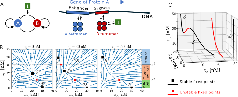
Figure 2: Example 1: Model of regulated stem cell differentiation. (A) Gene regulatory circuit. Left: Schematic of circuit showing upregulation (arrows), down regulation (flat arrows), and the effect of signaling molecule 1 concentration $c_{1}$ on amplification of the downregulation of ${\rm A}$ by ${\rm B}$. Right: Diagram of molecular mechanisms. Black arrows indicate molecular binding and unbinding of the A and B tetramers to the enhancer and silencer, and of signaling molecule 1 (green square) to B tetramer. Signaling molecule 2 controls cell proliferation and is not featured in this picture of individual-cell gene regulation dynamics. (B) Vector field $\bm{F}({\bm{z}};{\bm{c}})$ at three values of $c_{1}$. Attractors (black squares) are labelled by cell type: stem cells $\mathcal{S}$, triggered stem cells $\mathcal{S}^{*}$, and differentiated cells $\mathcal{D}$. Unstable fixed points indicated by red squares. Black dashed lines at $z_{\text{B}}=z^{\mathcal{S}}$ and $z^{\mathcal{D}}$ denote the boundary between stem cells and triggered stem, and between triggered stem cells and differentiated cells, respectively. (C) Fixed points of $\bm{F}({\bm{z}};{\bm{c}})$ as a function of $c_{1}$. Two saddle-node bifurcations result in the gain/loss of attractors $\mathcal{S}$ and $\mathcal{S}^{*}$.

The gene regulatory circuit that governs the dynamics of ${\bm{z}}$ is illustrated in Fig. 2A. Each gene (A and B) upregulates itself and downregulate the other. We make the common quasi-steady state assumption that mRNA transcription and degradation are fast relative to protein translation and degradation, so the state and dynamics are described in terms of only the protein concentrations ${\bm{z}}=(z_{\rm A},z_{\rm B})$. Signaling molecule “1” influences expression of gene A, but not gene B. Specifically, B tetramer (which downregulates gene A) can form a complex with signaling molecule 1, and this complex prevents any expression of A when bound to the silencer of A. This binding scheme gives rise to a Waddington vector field, shown in Fig. 2B, whose components are

$$F_{m}({\bm{z}};{\bm{c}})= r_{0,m}\big{(}1-E_{m}(z_{m})\big{)}\big{(}1-S_{m}(z_{m^{\prime}})\big{)}$$ (16)

$$\,\,+r_{E,m}E_{m}(z_{m})\big{(}1-S_{m}(z_{m^{\prime}})\big{)}$$

$$\,\,+r_{S,m}(c_{1})\big{(}1-E_{m}(z_{m})\big{)}S_{m}(z_{m^{\prime}})$$

$$\,\,+r_{ES,m}(c_{1})E_{m}(z_{m})S_{m}(z_{m^{\prime}})-k_{m}z_{m}$$

where $m,m^{\prime}=A,B$ or $B,A$. $E_{m}(z_{m})$ and $S_{m}(z_{m^{\prime}})$ are, respectively, the probabilities that the enhancer and silencer of gene $m$ have a bound tetramer, and are modeled by Hill functions:

$$E_{m}(z_{m})=\frac{z_{m}^{4}}{K_{E,m}^{4}+z_{m}^{4}},\,\,\,S_{m}(z_{m^{\prime}})=\frac{z_{m^{\prime}}^{4}}{K_{S,m}^{4}+z_{m^{\prime}}^{4}}.$$ (17)

The rates $r_{0,m}$, $r_{E,m}$, $r_{S,m}(c_{1})$, and $r_{ES,m}(c_{1})$ are the mean expression rates of gene $m$ with, respectively, neither enhancer nor silencer occupied, only enhancer occupied, only silencer occupied, and both enhancer and silencer occupied. The rates $r_{S,A}(c_{1})$ and $r_{ES,A}(c_{1})$ have a Michaelis-Menten type dependence on $c_{1}$:

$$r_{S,A}(c_{1})=\frac{r_{S,A}(0)\gamma}{\gamma+c_{1}},\quad r_{ES,A}(c_{1})=\frac{r_{ES,A}(0)\gamma}{\gamma+c_{1}}.$$ (18)

The factor $\gamma/(\gamma+c_{1})$ is the probability that a given B tetramer is not bound to a signaling molecule. All other rate parameters, $r_{0,m}$, $r_{E,m}$, $r_{S,B}$, $r_{ES,B}$, $r_{S,A}(0)$, and $r_{ES,A}(0)$ are constants (listed in Table 1, along with all other model parameters). Fig.  2B shows the Waddington vector field for three values of $c_{1}$: $c_{1}=0$ (left), $c_{1}=30$nM (middle), and $c_{1}=50$nM (right). For a particular choice of parameters, $\bm{F}({\bm{z}};{\bm{c}})$ reduces to the model in [55, 14].

The key role of signaling molecule $1$ is to regulate how stem cells are triggered for differentiation. Fig. 2B shows the attractors (black squares) for the three cell types ($\mathcal{S}$, $\mathcal{S}^{*}$, and $\mathcal{D}$). At intermediate $c_{1}$, stable attractors exist for both $\mathcal{S}$ and $\mathcal{S}^{*}$, but when $c_{1}$ drops sufficiently low, the $\mathcal{S}$ attractor disappears and stem cells move toward the triggered state $\mathcal{S}^{*}$. Hence, low $c_{1}$ triggers stem cells for differentiation, and as we will see below, these triggered stem cells undergo asymmetric division to produce differentiated cells. On the other hand, very high $c_{1}$ reverses the triggering (the $\mathcal{S}^{*}$ attractor disappears, so triggered stem cells revert to untriggered stem cells). Fig. 2C shows how the locations of the attractors (black) and unstable fixed points that separate the attractors (red) vary continuously with $c_{1}$. The unstable fixed point that separates the $\mathcal{S}$ and $\mathcal{S}^{*}$ attractors merges with $\mathcal{S}$ at low $c_{1}$, but merges with $\mathcal{S}^{*}$ at high $c_{1}$. These mergers of fixed points are saddle-node bifurcations.

Cell division rates depend on both the expression level $z_{\rm B}$ of protein B and the concentration $c_{2}$ of signaling molecule 2. The dependence on $z_{\rm B}$ gives rise to the defining behavior of the three cell types: stem cells divide symmetrically (both daughters are type $\mathcal{S}$), triggered stem cells divide asymmetrically (one daughter is $\mathcal{S}$ and the other $\mathcal{D}$), and differentiated cells do not divide. Mathematically, we model the birth rate by

$$\tilde{\beta}({\bm{z}};{\bm{z}}^{\prime},{\bm{z}}^{\prime\prime})=\hskip-2.84526pt\begin{cases}0&z_{\rm B}\leq z^{\mathcal{D}}\\[5.0pt] {\small\beta_{\mathcal{S}^{*}}\delta({\bm{z}}-{\bm{z}}^{\prime}-\bm{w}({\bm{z}}))}\\ \>\quad{\small\times\delta({\bm{z}}-{\bm{z}}^{\prime\prime}+\bm{w}({\bm{z}}))}&z^{\mathcal{S}}\!\geq z_{\rm B}\!>z^{\mathcal{D}}\\[6.0pt] \displaystyle\frac{a_{1}\delta({\bm{z}}-{\bm{z}}^{\prime})\delta({\bm{z}}-{\bm{z}}^{\prime\prime})}{1+a_{2}\exp(a_{3}c_{2})}&z_{\rm B}>z^{\mathcal{S}}.\end{cases}$$ (19)

where $z^{\mathcal{D}}<z^{\mathcal{S}}$ are threshold values for $z_{\rm B}$. Note that we do not include the $\Delta\bm{r}^{\prime},\Delta\bm{r}^{\prime\prime}$ dependencies because this model assumes a well-mixed (spatially uniform) system. The threshold concentrations $z^{\mathcal{S}}$ and $z^{\mathcal{D}}$ are indicated by dashed lines in Fig. 2B, and are determined by the (approximate) $z_{\rm B}$ values of the unstable fixed points of $\bm{F}$.

The vector $\bm{w}({\bm{z}})$ induces asymmetric division: when a triggered stem cell divides, one daughter has a state shifted by $\bm{w}({\bm{z}})$ relative to the mother, and the other daughter has state shifted by $-\bm{w}({\bm{z}})$. As a result, one daughter returns to the $\mathcal{S}$ attractor, while the other moves to the $\mathcal{D}$ attractor. Note that for ${\bm{z}}$ defined by concentrations, the concentrations ${\bm{z}}^{\prime}$ and ${\bm{z}}^{\prime\prime}$ in the daughter cells are related to that of the mother through $({\bm{z}}^{\prime}+{\bm{z}}^{\prime\prime})/2={\bm{z}}$. The death rate $\mu$ for all cells is assumed constant.

In this model, signaling molecule 1 is excreted by differentiated cells and signaling molecule 2 is excreted by stem cells. We use Eq. 9 to model signaling molecule concentrations, which assumes a well-mixed population and that concentrations rapidly reach steady state. The excretion rates of $c_{1}$ and $c_{2}$ are, respectively,

$$\bar{\lambda}_{1}({\bm{z}})=\begin{cases}0&z_{\rm B}>z^{\mathcal{D}}\\ L_{1}&z_{\rm B}\leq z^{\mathcal{D}}\end{cases}$$ (20)

and

$$\bar{\lambda}_{2}({\bm{z}})=\begin{cases}L_{2}&z_{\rm B}>z^{\mathcal{S}}\\ 0&z_{\rm B}\leq z^{\mathcal{S}}\end{cases}$$ (21)

Thus, according to Eq. 9, in a tissue with $N_{\mathcal{S}}$ stem cells and $N_{\mathcal{D}}$ differentiated cells, the concentrations are simply proportional to the cell numbers $n_{\mathcal{S}}$ and $n_{\mathcal{D}}$,

$$(c^{\rm ss}_{1},c^{\rm ss}_{2})=\Big{(}n_{\mathcal{D}}\mfrac{L_{1}}{d_{1}},n_{\mathcal{S}}\mfrac{L_{2}}{d_{2}}\Big{)}.$$ (22)

The signaling molecules’ influence on gene dynamics and birth rates gives rise to robust tissue development: from a wide range of initial conditions, the system dynamically approaches a stable tissue state with regulated relative cell type populations, as illustrated in Fig. 3A. The two signaling molecules govern the two key regulatory mechanisms: (i) the stem cell population, $n_{\mathcal{S}}$, is self-regulated due to the dependence of stem cell division on $c_{2}$. When $n_{\mathcal{S}}$ is low (high), $c_{2}$ is low (high), so stem cell division rate is high (low), replenishing (diminishing) $n_{\mathcal{S}}$ towards the stable, developed state; (ii) the dependence of $\bm{F}({\bm{z}};{\bm{c}})$ on $c_{1}$ leads to a thermostat-like behavior of stem cell triggering. When $n_{\mathcal{D}}$ is low (high), $c_{1}$ is low (high), so more (less) stem cells are triggered for asymmetric division. This thermostat-like behavior is apparent from Fig. 3A; whenever $n_{\mathcal{D}}$ drops below a threshold, stem cells are triggered, rapidly replenishing $n_{\mathcal{D}}$. In Fig. 3A specifically, an initial population of only four stem cells develops into the stable tissue state.

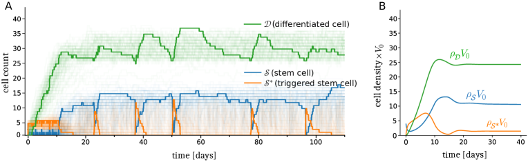
Figure 3: Example 1: Dynamics of cell populations. (A) Dynamical simulation starting from an initial condition with $N_{\cal S}=4$ and $N_{{\cal S}^{*}}=N_{D}=0$. The population dynamics exhibit thermostat-like behavior: when $N_{\cal D}$ falls below 26, stem cells are triggered for asymmetric division, which results in $N_{\cal D}$ being replenished. One-hundred trajectories were simulated by evaluating Eq. 1, coupled with a discrete cell birth-death process, using the standard Euler-Maruyama method. One representative trajectory is highlighted, while the other ninety-nine are lightly shaded. (B) Evolution of cell populations in the deterministic limit. The densities are multiplied by the normalizing volume $V_{0}$ to express densities on the same scale as particle counts. Note that the deterministic trajectories qualitatively reflect the overall dynamics shown in (A).

V.1 Deterministic limit

The deterministic limit described in section III.6 can be applied to obtain a highly simplified form of the model. Denote the cell densities for the three cell types as $\bm{\rho}=(\rho_{\mathcal{S}},\rho_{\mathcal{S}^{*}},\rho_{\mathcal{D}})$. The developmental fitness landscape is

$$\bm{\phi}({\bf n})=\big{(}\beta_{\mathcal{S}}(n_{\mathcal{S}})-F_{\mathcal{D},\mathcal{S}}(n_{\mathcal{D}}){-}\mu,\,\,-\beta_{\mathcal{S}^{*}}{-}\mu,\,\,-\mu\big{)}$$ (23)

where $\beta_{\mathcal{S}}(n_{\mathcal{S}})\equiv a_{1}/(1+a_{2}\exp{(a_{3}n_{\mathcal{S}}L_{2}/d_{2})})$, as determined by Eqs. 19 and 22. $F_{\mathcal{D},\mathcal{S}}(n_{\mathcal{D}})$ is the rate at which stem cells are triggered. $F_{\mathcal{D},\mathcal{S}}(n_{\mathcal{D}})$ can be estimated numerically by simulating the gene dynamics, and it is well approximated by a step function, equal to 0 for $n_{\mathcal{D}}>25$ and greater than 0 for $n_{\mathcal{D}}\leq 25$. The deterministic equations given by Eq. 12 written out explicitly are

$$\frac{\mbox{d}\rho_{\mathcal{S}}}{\mbox{d}t} =\big{(}\beta_{\mathcal{S}}(\rho_{\mathcal{S}}V_{0})-F_{\mathcal{D},\mathcal{S}}(\rho_{\mathcal{D}}V_{0})-\mu\big{)}\rho_{\mathcal{S}}+\beta_{\mathcal{S}^{*}}\rho_{\mathcal{S}^{*}}$$ (24)

$$\frac{\mbox{d}\rho_{\mathcal{S}^{*}}}{\mbox{d}t} =F_{\mathcal{D},\mathcal{S}}(\rho_{\mathcal{D}}V_{0})\rho_{\mathcal{S}}-\big{(}\beta_{\mathcal{S}^{*}}+\mu\big{)}\rho_{\mathcal{S}^{*}}$$

$$\frac{\mbox{d}\rho_{\mathcal{D}}}{\mbox{d}t} =\beta_{\mathcal{S}^{*}}\rho_{\mathcal{S}^{*}}-\mu\rho_{\mathcal{D}}.$$

Fig. 3B plots the solutions of these equations for the same initial conditions as in Fig. 2D. The transient thermostat-like behavior is lost, but the longer timescale results are qualitatively similar.

VI Example 2: Spatial model inspired by planaria

Here, we present a model of a spatially-structured multicellular organism which develops from a single cell. Additionally, if the developed organism is cut into pieces, each piece will regenerate into a new fully-developed organism (a phenomenon called fissiparous reproduction). This model is inspired by planaria worms, which exhibit a remarkable capacity for fissiparous reproduction: a fragment of a planarian as small as 1/279th of the full worm can regenerate into a new worm [56, 57].

In this model, cell state is described by the expression of a single gene, denoted gene A, whose expression is governed by a bistable regulatory circuit. The state $z$ is the concentration of protein A (we assume fast mRNA dynamics, as in example 1). Two stable states corresponding to two values of $z$ define two cell types: exterior cells (which have low $z$) and interior cells (which have high $z$). Cells excrete two signaling molecules, one which governs the $z$ dynamics and another which governs cell division rate. The cells live and migrate on a 2D substrate ($\bm{r}\in\mathbb{R}^{2}$), and they exert forces on one another which govern their movement.

The gene regulatory circuit is illustrated in Fig. 4A. Gene A upregulates itself when signaling molecule 1 is present. Specifically, protein A can bind to signaling molecule 1, and this heterodimer binds to the enhancer of gene A, increasing the expression of protein A. The Waddington vector field thus takes the form

$$F(z;c)=r_{0}+\frac{r_{1}c_{1}z^{2}}{K^{2}+z^{2}}-bz.$$ (25)

The values of the parameters $r_{0}$, $r_{1}$, $K$, and $b$, as well of the parameters introduced in the following equations, are given in Table 1.

Figure 4: Example 2: Model of a spatially structured organism with fissiparous reproduction. (A) Gene regulatory circuit, where gene A upregulates itself in the presence of signaling molecule 1. (B) Waddington vector field (blue arrows), attractors (black curves) and unstable fixed points (red curve) as a function of $c_{1}$. The lefthand attractor represents exterior cells and the righthand attractor represents interior cells. (C) Simulation of the dynamics, showing a single cell developing into a stable developed organism (day 0 through 4). At time $t=4.0$ days, the organism is bisected and the left half is removed. The organism then regrows (4.1 to 6.0 days). Top row: cell position (black dots) and the state level $z$ given by the color shading. Middle and bottom rows depict the corresponding concentrations $c_{1}$ and $c_{2}$, respectively.

Fig. 4B shows the dynamics (blue arrows) as well as the locations of the attractors (black) and unstable fixed points (red) of $F(z;c)$, for values of $c_{1}$ between 4 and 12 nM. The attractor at low (high) $z$, which corresponds to exterior (interior) cells, merges with the unstable fixed point at high (low) $c_{1}$ via a saddle-node bifurcation; when $c_{1}$ reaches this bifurcation, exterior (interior) cells convert to interior (exterior) cells. In this way, cell type is regulated by $c_{1}$.

Cell movement is described by Eq. 3 with

$$\bm{g}(\bm{r}^{\alpha},S)=\sum_{\alpha^{\prime}\neq\alpha}\bm{v}(\bm{r}^{\alpha}-\bm{r}^{\alpha^{\prime}})$$ (26)

where $\bm{v}(\bm{r})=v_{0}(\frac{r_{\text{min}}^{2}}{r^{3}}-\frac{r_{\text{min}}}{r^{2}})\bm{\hat{r}}$, where $\bm{\hat{r}}$ is the unit vector in the $\bm{r}$ direction and $v_{0}$ is a parameter that sets the velocity scale (see Table 1). We assume the motion is deterministic, so $\eta=0$ in Eq. 3. The velocity $\bm{v}(\bm{r})$ moves cells separated by a distance greater than $r_{\text{min}}$ closer together (e.g., response to an attractive force), but moves cells separated by less than $r_{\text{min}}$ further apart, corresponding to a close-ranged repulsive force. Hence, the cells that comprise the tissue adhere together with an average spacing of approximately $r_{\text{min}}$.

The spatial profile of signaling molecule concentrations is key to the regulation of cell number and cell type. We assume rapid equilibration of signaling molecule concentrations (section III.1), with $c_{\ell}^{\text{ss}}$ given by Eq. 6 with $z$-independent $c^{(1)}_{\ell}(\bm{r})=C_{\ell}\exp\big{(}-r^{2}/(2s_{\ell}^{2})\big{)}$ for $\ell=1,2$ and $r=|\bm{r}|$. While the concentration field $c^{(1)}_{\ell}(\bm{r})$ due to a single cell can be computed from Eq. 7, it can also be well-approximated by a Gaussian spread function with appropriately chosen variance $s_{\ell}^{2}$ (see Table 1). The concentration $c_{1}$ informs cells as to whether they are surrounded by many (high $c_{1}$) or few (low $c_{1}$) neighboring cells. The gene regulatory circuit ensures that cells with many neighbors become interior cells and cells with fewer neighbors become exterior cells.

As in Example 1, the concentration of molecule 2, $c_{2}$, mediates the total cell population by influencing cell division rates, which we model by

$$\tilde{\beta}({\bm{c}};\Delta\bm{r}^{\prime},\Delta\bm{r}^{\prime\prime})=\begin{cases}\beta_{0}\delta(\Delta\bm{r}^{\prime}){\cal N}(\Delta\bm{r}^{\prime\prime})&c_{2}<c_{2}^{*}\\ 0&c_{2}\geq c_{2}^{*},\end{cases}$$ (27)

where ${\cal N}(\bm{r})\equiv\frac{1}{2\pi\xi^{2}}e^{-\bm{r}^{2}/2\xi^{2}}$ is the 2-dimensional Gaussian density function with variance $\xi^{2}$. Note that the division rate is independent of $z$.

Fig. 4C shows a simulation of the model. Starting from a single cell at $t=0$, the organism grows into a fully-developed organism in roughly four days. For approximately the first two days, all cells are of the exterior type (purple). After the organism grows sufficiently large that $c_{1}$ concentration reaches a sufficient level, conversion to interior-type cells (yellow) occurs. In Fig. 4C, the top row indicates the positions and $z$-states of cells, the middle row shows signaling molecule 1 concentrations, and the bottom row shows signaling molecule 2 concentrations.

If the fully developed organism is bisected, each half regrows. In the simulation shown in Fig. 4C, the organism is bisected at time $t=4.0$ days along the dotted line shown in the figure, and the righthand portion is removed. The remaining lefthand portion then regrows into a new fully-developed organism in approximately 2 days. These results illustrate an extremely robust developmental process.

Table 1: Model Parameters for Examples 1 and 2.

Parameter	Value	[units]	Description
Example 1 Model Parameters
$a_{1}$	1	[day-1]	Max. stem cell division rate (Eq. 19)
$a_{2}$	0.15	[unitless]	Parameter in Eq. 19
$a_{3}$	0.5	[unitless]	Parameter in Eq. 19
$\beta_{\mathcal{S}^{*}}$	0.6	[day-1]	Triggered stem cell division rate (Eq. 19)
$\bm{w}({\bm{z}})$	$0.95(z_{\rm A},-z_{\rm B})$	$[z]$	Controls asymmetric division (Eq. 19)
$\mu$	0.02	[day-1]	Death rate
$L_{1}$, $L_{2}$	1	[nM]	Mean excretion rates of signaling molecules (Eqs. 20, 21)
$z^{\mathcal{S}}$	15	[nM]	Threshold value of $z_{\text{B}}$ between stem cells and triggered stem cells (Eqs. 19, 21)
$z^{\mathcal{D}}$	5	[nM]	Threshold value of $z_{\text{B}}$ between triggered stem and differentiated cells (Eqs. 19, 20)
$K_{E,m}$	5	[nM]	Equilibrium const. for tetramerization and binding of $m$=A, B to Enhancer (Eq. 17)
$K_{S,m}$	5	[nM]	Equilibrium const. for tetramerization and binding of $m$=A, B to Silencer (Eq. 17)
$\gamma$	20	[nM]	Equilibrium const. for signaling molecule 1 binding to B tetramer (Eq. 18)
$r_{0,A}$	500	[nM/day]	Expression rate of A when A enhancer and silencer of A are unoccupied (Eq. 16)
$r_{0,B}$	500	[nM/day]	Expression rate of B when B enhancer and silencer of B are unoccupied (Eq. 16)
$r(0)_{S,A}$	250	[nM/day]	Expression rate of A when A silencer is occupied and $c_{1}=0$ (Eq. 18)
$r(0)_{ES,A}$	1000	[nM/day]	Expression rate of A when A enhancer and silencer are occupied and $c_{1}=0$ (Eq. 18)
$r_{E,A}$	1500	[nM/day]	Expression rate of A when A enhancer is occupied (Eq. 16)
$r_{E,B}$	1000	[nM/day]	Expression rate of B when B enhancer is occupied (Eq. 16)
$r_{S,B}$	0	[nM/day]	Expression rate of B when B silencer is occupied (Eq. 16)
$r_{ES,B}$	500	[nM/day]	Expression rate of B when B enhancer and silencer are occupied (Eq. 16)
$k_{m}$	50	[day-1]	Degradation rate of $m$=A, B (Eq. 16)
$\sigma({\bm{z}};{\bm{c}})$	$0.1\begin{bmatrix}z_{\text{A}}&0\\ 0&z_{\text{B}}\end{bmatrix}$	[day-1/2]	Noise magnitude of gene dynamics (Eq. 1)
Example 2 Model Parameters
$\beta_{0}$	1	[day-1]	Division rate (Eq. 27)
$\xi$	2.5	[$\mu$m]	Std. dev. of displacement of daughter from mother (below Eq. 27)
$c_{2}^{*}$	23	[nM]	Threshold of $c_{2}$ above which cell division does not occur (Eq. 27)
$\mu$	0.1	[day-1]	Death rate
$C_{\ell}$	1	[nM]	Parameter controlling excretion rate of signaling molecule $\ell=1,2$
$s_{1}$	7	[$\mu$m]	Std. dev. of spatial profile of excretion of signaling molecule 1
$s_{2}$	30	[$\mu$m]	Std. dev. of spatial profile of excretion of signaling molecule 2
$r_{0}$	1000	[nM/day]	Expression rate of A when enhancer is unoccupied (Eq. 25)
$r_{1}$	2100	[nM/day]	Enhancement in expression rate when enhancer is occupied (Eq. 25)
$K$	35	[nM]	Equilibrium const. for dimerization and heterodimer-Enhancer binding (Eq. 25)
$b$	250	[day-1]	Degradation rate of protein A (Eq. 25)
$\sigma$	$0.1z$	[day-1/2]	Noise magnitude of gene dynamics (Eq. 1)
$v_{0}$	$10^{3}$	[$\mu$m2/day]	Parameter controlling velocity of cell movement (Eq. 26)
$r_{\text{min}}$	8	[$\mu$m]	Spatial extent of attractive forces between cells (Eq. 26)
$\eta$	0		Noise magnitude of cell movement (Eq. 3)

VII Summary and Conclusions

We have systematically constructed a general model for tissue development that incorporates intracellular gene expression dynamics, the effects of gene expression state on proliferation and death rates, heritability of cellular states during cell division, and cell-cell interactions via chemical signaling. Dissecting our interacting-cell framework into individual components, we provide a mathematically unambiguous definition of a “Waddington landscape” (described as a Waddington vector field to allow for nonequilibrium, driven dynamics) and, if cell states are discretized, a developmental “fitness landscape.”

Our general framework integrates submodels for four processes: stochastic changes in gene expression within each cell of the tissue (Eq. 1), chemical signals produced and received by cells affecting their gene expression dynamics (Eq. 2), spatial movement of cells (Eq. 3) which may affect their exposure to signaling molecules, and finally, stochastic cell proliferation (Eq. 10) that allows daughter cells to acquire different states than their mother (through the differential birth rate parameter function of Eq. 4). These distinct processes are coupled together through the chemical signaling field ${\bm{c}}$, the drift and diffusivity of cells (which may depend on cell state ${\bm{z}}$ and chemical field ${\bm{c}}$), and the differential birth rate which may also depend on mother-cell state and local chemical fields. These components represent an intermediate level of coarse-graining that allows for better interpretability than fine-grained computational models (such as CompuCell 3D [58]) or unwieldy kinetic theories [29, 30] that are difficult to marginalize to obtain equations for interpretable and measurable quantities, particularly if cells interact.

While the importance of cell-cell interactions and differential cell division and death rates for robust development is well understood [34, 59], the complexity of incorporating these features into mathematical models has been an obstacle in modeling studies. Many theoretical works study cell fate transitions for single cells [14, 13, 15, 8, 3, 16, 17, 18, 19, 20] or for populations of dividing but noninteracting cells without spatial structure [23, 24, 25, 26, 27, 28]. For example, cell-cell interactions mediated by a chemical signaling concentration field, as in Eq. 2, typically cannot be incorporated into kinetic equations [29, 30, 60] in a straightforward way. Models that include spatial structure governed by cell-cell interactions, but which do not incorporate tissue growth via coordinated cell division or death, have also been studied [38, 61]. The models developed in [5, 6] incorporate cell-cell interactions and differential cell division rates to describe coordinated tissue development; these models also provide a more detailed description of the cell cycle than our framework. However, unlike our framework, they describe the cell population as a continuous distribution of infinitely many cells rather than describing individual cells as discrete entities, and they do not incorporate spatial structure.

We applied our intermediate-grained stochastic dynamical framework to two biological canonical processes: stem cell differentiation in a well-mixed environment and a spatially-structured growth and regeneration process. While the examples in this work are simplified models intended to provide conceptual clarity of general mechanisms of robust tissue development, one should be able to apply our framework to many other developmental processes that involve chemical signaling such as morphogenesis, embryogenesis, organogenesis, and patterning [33, 62, 63].

Appendix A Mis-application of the Waddington Landscape Equations

The mis-application of Eqs. 14 and 15 to systems that are either non-gradient systems, or which have non-additive noise, can lead to artifacts in the reconstructed dynamics. As in Eq. 15, let $U_{R}({\bm{z}})=-\log p_{\rm ss}({\bm{z}})$ denote a reconstructed landscape where $p_{ss}({\bm{z}})$ is the steady state distribution of cell states generated by some stochastic dynamics $\mbox{d}{\bm{z}}=\bm{F}({\bm{z}})\mbox{d}t+\sigma({\bm{z}})\mbox{d}{\bf W}$. The reconstructed vector field $\bm{F}_{R}({\bm{z}})\equiv-\nabla U_{R}({\bm{z}})$ can have ‘false’ attractors (attractors that are absent in $\bm{F}({\bm{z}})$. An example of this is shown in Fig. 5A, with the false attractor indicated by a red square. Additionally, $\bm{F}_{R}({\bm{z}})$ may fail to have attractors that do exist in $\bm{F}({\bm{z}})$. An example of this is shown in Fig. 5B, with the true attractor that disappears in the reconstructed vector field indicated by an orange square.

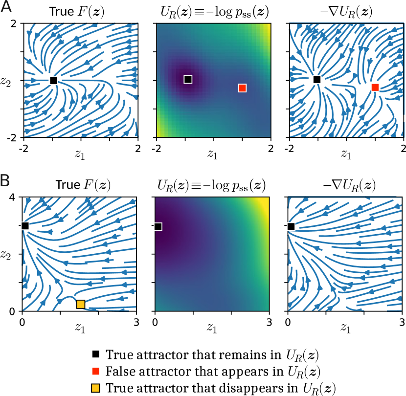
Figure 5: Artifacts due to the mis-application of Eqs. 14 and 15. (A) An example showing a false attractor (red square) which does not exist in the true vector field, but which appears in the reconstructed vector field. (B) An example showing a true attractor which disappears in the reconstructed vector field (orange square). The reconstructed landscapes $U_{R}({\bm{z}})$ are color coded where blue represents small values and yellow represents large values.

References

- [1] Conrad H Waddington. Canalization of development and the inheritance of acquired characters. Nature, 150(3811):563–565, 1942.
- [2] James E Ferrell. Bistability, bifurcations, and Waddington’s epigenetic landscape. Current Biology, 22(11):R458–R466, 2012.
- [3] Geoffrey Schiebinger. Reconstructing developmental landscapes and trajectories from single-cell data. Current Opinion in Systems Biology, 27:100351, 2021.
- [4] Leili Shahriyari and Natalia L Komarova. Symmetric vs. asymmetric stem cell divisions: an adaptation against cancer? PLoS ONE, 8(10):e76195, 2013.
- [5] Jinzhi Lei. A general mathematical framework for understanding the behavior of heterogeneous stem cell regeneration. Journal of Theoretical Biology, 492:110196, 2020.
- [6] Jinzhi Lei. Mathematical modeling of heterogeneous stem cell regeneration: from cell division to Waddington’s epigenetic landscape. arXiv preprint arXiv:2309.08064, 2023.
- [7] Jin Wang, Li Xu, and Erkang Wang. Potential landscape and flux framework of nonequilibrium networks: robustness, dissipation, and coherence of biochemical oscillations. Proceedings of the National Academy of Sciences, 105(34):12271–12276, 2008.
- [8] David A Rand, Archishman Raju, Meritxell Sáez, Francis Corson, and Eric D Siggia. Geometry of gene regulatory dynamics. Proceedings of the National Academy of Sciences, 118(38):e2109729118, 2021.
- [9] Megan A Coomer, Lucy Ham, and Michael PH Stumpf. Noise distorts the epigenetic landscape and shapes cell-fate decisions. Cell Systems, 13(1):83–102, 2022.
- [10] Meritxell Sáez, Robert Blassberg, Elena Camacho-Aguilar, Eric D Siggia, David A Rand, and James Briscoe. Statistically derived geometrical landscapes capture principles of decision-making dynamics during cell fate transitions. Cell Systems, 13(1):12–28, 2022.
- [11] Peijie Zhou and Tiejun Li. Construction of the landscape for multi-stable systems: Potential landscape, quasi-potential, A-type integral and beyond. The Journal of Chemical Physics, 144(9), 2016.
- [12] Archishman Raju, BingKan Xue, and Stanislas Leibler. A theoretical perspective on Waddington’s genetic assimilation experiments. Proceedings of the National Academy of Sciences, 120(51):e2309760120, 2023.
- [13] Daniel R Sisan, Michael Halter, Joseph B Hubbard, and Anne L Plant. Predicting rates of cell state change caused by stochastic fluctuations using a data-driven landscape model. Proceedings of the National Academy of Sciences, 109(47):19262–19267, 2012.
- [14] Jin Wang, Kun Zhang, Li Xu, and Erkang Wang. Quantifying the Waddington landscape and biological paths for development and differentiation. Proceedings of the National Academy of Sciences, 108(20):8257–8262, 2011.
- [15] Atefeh Taherian Fard, Sriganesh Srihari, Jessica C Mar, and Mark A Ragan. Not just a colourful metaphor: modelling the landscape of cellular development using Hopfield networks. NPJ Systems Biology and Applications, 2(1):1–9, 2016.
- [16] Xiaojie Qiu, Yan Zhang, Jorge D Martin-Rufino, Chen Weng, Shayan Hosseinzadeh, Dian Yang, Angela N Pogson, Marco Y Hein, Kyung Hoi Joseph Min, Li Wang, et al. Mapping transcriptomic vector fields of single cells. Cell, 185(4):690–711, 2022.
- [17] Anna-Simone Josefine Frank, Kamila Larripa, Hwayeon Ryu, and Susanna Röblitz. Macrophage phenotype transitions in a stochastic gene-regulatory network model. Journal of Theoretical Biology, 575:111634, 2023.
- [18] Yoshiyuki T Nakamura, Yusuke Himeoka, Nen Saito, and Chikara Furusawa. Evolution of hierarchy and irreversibility in theoretical cell differentiation model. PNAS NEXUS, 3(1):pgad454, 2024.
- [19] Gang Xue, Xiaoyi Zhang, Wanqi Li, Lu Zhang, Zongxu Zhang, Xiaolin Zhou, Di Zhang, Lei Zhang, and Zhiyuan Li. A logic-incorporated gene regulatory network deciphers principles in cell fate decisions. Elife, 12:RP88742, 2024.
- [20] Xinxin Chen, Ying Sheng, Liang Chen, Moxun Tang, and Feng Jiao. Quantifying cell fate change under different stochastic gene activation frameworks. Quantitative Biology, 13(1):e82, 2025.
- [21] Weikang Wang, Dante Poe, Yaxuan Yang, Thomas Hyatt, and Jianhua Xing. Epithelial-to-mesenchymal transition proceeds through directional destabilization of multidimensional attractor. eLife, 11:e74866, feb 2022.
- [22] Weikang Wang, Ke Ni, Dante Poe, and Jianhua Xing. Transiently increased coordination in gene regulation during cell phenotypic transitions. PRX Life, 2:043009, 2024.
- [23] Caleb Weinreb, Samuel Wolock, Betsabeh K Tusi, Merav Socolovsky, and Allon M Klein. Fundamental limits on dynamic inference from single-cell snapshots. Proceedings of the National Academy of Sciences, 115(10):E2467–E2476, 2018.
- [24] David S Fischer, Anna K Fiedler, Eric M Kernfeld, Ryan MJ Genga, Aimée Bastidas-Ponce, Mostafa Bakhti, Heiko Lickert, Jan Hasenauer, Rene Maehr, and Fabian J Theis. Inferring population dynamics from single-cell rna-sequencing time series data. Nature Biotechnology, 37(4):461–468, 2019.
- [25] Jifan Shi, Tiejun Li, Luonan Chen, and Kazuyuki Aihara. Quantifying pluripotency landscape of cell differentiation from scRNA-seq data by continuous birth-death process. PLoS Computational Biology, 15(11):e1007488, 2019.
- [26] Stephen Zhang, Anton Afanassiev, Laura Greenstreet, Tetsuya Matsumoto, and Geoffrey Schiebinger. Optimal transport analysis reveals trajectories in steady-state systems. PLoS Computational Biology, 17(12):e1009466, 2021.
- [27] Aden Forrow and Geoffrey Schiebinger. LineageOT is a unified framework for lineage tracing and trajectory inference. Nature Communications, 12(1):4940, 2021.
- [28] Jifan Shi, Kazuyuki Aihara, Tiejun Li, and Luonan Chen. Energy landscape decomposition for cell differentiation with proliferation effect. National Science Review, 9(8):nwac116, 2022.
- [29] Mingtao Xia and Tom Chou. Kinetic theory for structured populations: application to stochastic sizer-timer models of cell proliferation. Journal of Physics A: Mathematical and Theoretical, 54(38):385601, 2021.
- [30] Mingtao Xia and Tom Chou. Kinetic theories of state- and generation-dependent cell populations. Physical Review E, 110:064146, 2024.
- [31] Chris D. Greenman and Tom Chou. Kinetic theory of age-structured stochastic birth-death processes. Physical Review E, 93:012112, 2016.
- [32] Tom Chou and Chris D. Greenman. A hierarchical kinetic theory of birth, death and fission in age-structured interacting populations. J. Stat. Phys., 164:49–76, 2016.
- [33] Michael Barresi and Scott Gilbert. Developmental Biology, 13th Ed. Oxford University Press, 2023.
- [34] Dennis E Discher, David J Mooney, and Peter W Zandstra. Growth factors, matrices, and forces combine and control stem cells. Science, 324(5935):1673–1677, 2009.
- [35] Sui Huang. Genetic and non-genetic instability in tumor progression: link between the fitness landscape and the epigenetic landscape of cancer cells. Cancer and Metastasis Reviews, 32:423–448, 2013.
- [36] Sui Huang. Reconciling non-genetic plasticity with somatic evolution in cancer. Trends in Cancer, 7(4):309–322, 2021.
- [37] The labeling of cells is arbitrary. One straightforward labeling scheme is to label cells from oldest to youngest, i.e., cell is the oldest cell. When a cell dies, all cells younger than the dying cell are then re-labeled.
- [38] Hosein Fooladi, Parsa Moradi, Ali Sharifi-Zarchi, and Babak Hosein Khalaj. Enhanced Waddington landscape model with cell–cell communication can explain molecular mechanisms of self-organization. Bioinformatics, 35(20):4081–4088, 2019.
- [39] Niraj Kumar, Thierry Platini, and Rahul V. Kulkarni. Exact distributions for stochastic gene expression models with bursting and feedback. Phys. Rev. Lett., 113:268105, 2014.
- [40] Chen Jia and Ramon Grima. Small protein number effects in stochastic models of autoregulated bursty gene expression. The Journal of Chemical Physics, 152(8):084115, 2020.
- [41] Xinyu Wang, Youming Li, and Chen Jia. Poisson representation: a bridge between discrete and continuous models of stochastic gene regulatory networks. Journal of The Royal Society Interface, 20(208):20230467, 2023.
- [42] Daniel T Gillespie. Exact stochastic simulation of coupled chemical reactions. The Journal of Physical Chemistry, 81(25):2340–2361, 1977.
- [43] Daniel T Gillespie. The chemical Langevin equation. The Journal of Chemical Physics, 113(1):297–306, 2000.
- [44] Wang Xi, Thuan Beng Saw, Delphine Delacour, Chwee Teck Lim, and Benoit Ladoux. Material approaches to active tissue mechanics. Nature Reviews Materials, 4(1):23–44, 2019.
- [45] Jonas Ranft, Markus Basan, Jens Elgeti, Jean-Francois Joanny, Jacques Prost, and Frank Jülicher. Fluidization of tissues by cell division and apoptosis. Proceedings of the National Academy of Sciences, 107(49):20863–20868, 2010.
- [46] Sarah A Nowak, B Chakrabarti, Tom Chou, and Ajay Gopinathan. Frequency-dependent chemolocation and chemotactic target selection. Physical Biology, 7(2):026003, 2010.
- [47] Peter Dieterich, Rainer Klages, Roland Preuss, and Albrecht Schwab. Anomalous dynamics of cell migration. Proceedings of the National Academy of Sciences, 105(2):459–463, 2008.
- [48] Tajie H Harris, Edward J Banigan, David A Christian, Christoph Konradt, Elia D Tait Wojno, Kazumi Norose, Emma H Wilson, Beena John, Wolfgang Weninger, Andrew D Luster, et al. Generalized Lévy walks and the role of chemokines in migration of effector CD8+ T cells. Nature, 486(7404):545–548, 2012.
- [49] Felix Höfling and Thomas Franosch. Anomalous transport in the crowded world of biological cells. Reports on Progress in Physics, 76(4):046602, 2013.
- [50] Sumin Jang, Sandeep Choubey, Leon Furchtgott, Ling-Nan Zou, Adele Doyle, Vilas Menon, Ethan B Loew, Anne-Rachel Krostag, Refugio A Martinez, Linda Madisen, Boaz P Levi, and Sharad Ramanathan. Dynamics of embryonic stem cell differentiation inferred from single-cell transcriptomics show a series of transitions through discrete cell states. eLife, 6:e20487, 2017.
- [51] Peter Hänggi, Peter Talkner, and Michal Borkovec. Reaction-rate theory: fifty years after Kramers. Reviews of modern physics, 62(2):251, 1990.
- [52] R. Dessalles, M. D’Orsogna, and T. Chou. Exact steady-state distributions of multispecies birth–death–immigration processes: Effects of mutations and carrying capacity on diversity. J. Stat. Phys., 173:82–221, 2018.
- [53] Paras Jain, Ramanarayanan Kizhuttil, Madhav B Nair, Sugandha Bhatia, Erik W Thompson, Jason T George, and Mohit Kumar Jolly. Cell-state transitions and density-dependent interactions together explain the dynamics of spontaneous epithelial-mesenchymal heterogeneity. iScience, 2024.
- [54] Crispin W Gardiner. Handbook of stochastic methods for physics, chemistry and the natural sciences. Springer Series in Synergetics, 1985.
- [55] Sui Huang, Yan-Ping Guo, Gillian May, and Tariq Enver. Bifurcation dynamics in lineage-commitment in bipotent progenitor cells. Developmental Biology, 305(2):695–713, 2007.
- [56] Thomas Hunt Morgan. Experimental studies of the regeneration of Planaria maculata, volume 2. W. Engelmann, 1898.
- [57] Daniel Lobo, Wendy S Beane, and Michael Levin. Modeling planarian regeneration: a primer for reverse-engineering the worm. PLoS Computational Biology, 8(4):e1002481, 2012.
- [58] M. Swat, Gilberto L. Thomas, Julio M. Belmonte, A. Shirinifard, D. Hmeljak, and J. A. Glazier. Multi-scale modeling of tissues using compuCell3D. Computational Methods in Cell Biology, Methods in Cell Biology, 110:325–366, 2012.
- [59] Benoit G Godard and Carl-Philipp Heisenberg. Cell division and tissue mechanics. Current Opinion in Cell Biology, 60:114–120, 2019.
- [60] Mingtao Xia, Xiangting Li, and Tom Chou. Overcompensation of transient and permanent death rate increases in age-structured models with cannibalistic interactions. Physica D: Nonlinear Phenomena, 470:134339, 2024.
- [61] Matthew Smart and Anton Zilman. Emergent properties of collective gene-expression patterns in multicellular systems. Cell Reports Physical Science, 4(2), 2023.
- [62] Jeremy B. A. Green and James Sharpe. Positional information and reaction-diffusion: two big ideas in developmental biology combine. Development, 142(7):1203–1211, 04 2015.
- [63] Hans Meinhardt. Hierarchical inductions of cell states: A model for segmentation in Drosophila. Journal of Cell Science, 1986:357–381, 1986.