tcb@breakable
A Metric Topology of Deep Learning for Data Classification
Abstract
Empirically, Deep Learning (DL) has demonstrated unprecedented success in practical applications. However, DL remains by and large a mysterious “black-box”, spurring recent theoretical research to build its mathematical foundations. In this paper, we investigate DL for data classification through the prism of metric topology. Considering that conventional Euclidean metric over the network parameter space typically fails to discriminate DL networks according to their classification outcomes, we propose from a probabilistic point of view a meaningful distance measure, whereby DL networks yielding similar classification performances are close. The proposed distance measure defines such an equivalent relation among network parameter vectors that networks performing equally well belong to the same equivalent class. Interestingly, our proposed distance measure can provably serve as a metric on the quotient set modulo the equivalent relation. Then, under quite mild conditions it is shown that, apart from a vanishingly small subset of networks likely to predict non-unique labels, our proposed metric space is compact, and coincides with the well-known quotient topological space. Our study contributes to fundamental understanding of DL, and opens up new ways of studying DL using fruitful metric space theory.
Index Terms:
deep learning, classification, equivalent relation, metric space, compactness, quotient topologyI Introduction
I-A Background and paper contributions
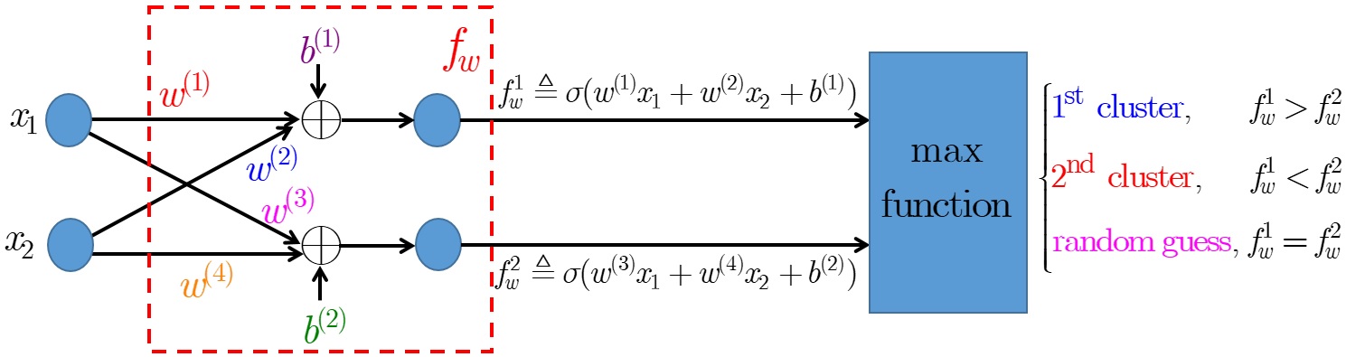
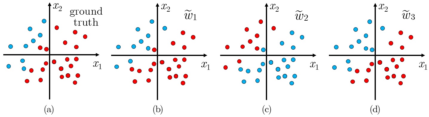
Deep learning (DL) is epoch-making and its study grows apace in the recent years [1, 2]. Despite phenomenal empirical performances having been demonstrated in many application domains, less is known about the theoretical side. Investigation into mathematics of DL is therefore underway, from training/architecture optimization [3, 4, 5, 6], generalization error analysis [7, 8, 9, 10], to interplay with quantum physics [11, 12, 13], towards building mathematical foundations underlying its sheer success. Our study in this paper is in pursuit of fundamental understanding of DL tasked with data classification, and is well motivated by the toy example given below. Consider a one-layer DL network consisting of six real parameters responsible for binary classification over , as depicted in Fig. 1; three distinct network parameter vectors , along with their pair-wise Euclidean distances, are then listed in Table I. For randomly sampled testing points, the labels output by are shown in Fig. 2, in which close network parameter vectors (say, and because , less than and ) are seen to perform nonetheless drastically different. Obviously, the Euclidean metric fails to discriminate networks according to their classification outcomes. This then inspires construction of a meaningful metric, against which DL networks yielding similar data classification performance are close. Not only can such a metric (if available) offer accurate performance assessment, but also give birth to a potential metric topology underlying DL for data classification, enriching theoretical research of DL with fruitful metric space theory [14, 15, 16].
| 0.283 | 3.959 | 4.243 |
In light of the above points, the main contributions of this paper can be summarized as follows.
-
1.
We propose a new distance measure from a probabilistic point of view, against which DL networks delivering similar classification outcomes are close. Conceptually, our proposed solution gauges the likelihood that the decisions of two networks disagree; in particular, the distance from a given DL network to the ground truth classifier turns out to be its generalization error [17, 8, 9, 18].
-
2.
We show the distance measure defines such an equivalent relation that networks yielding identical performances belong to the same equivalent class. The associated quotient set modulo the equivalent relation, therefore, is composed of disjoint equivalent classes, each one consisting of DL networks performing equally well.
-
3.
Importantly, our distance measure can provably serve as a metric on the quotient set. Under quite mild assumptions on the input data distribution it is shown that, apart from a vanishingly small subset of networks likely to predict non-unique labels, the proposed metric space is compact.
-
4.
Finally, it is shown that the proposed metric topology on the quotient set coincides with the well-known quotient topology [19], namely, the collection of all subsets of the quotient set whose inverse images under the projection map [20], in our case from the Euclidean network parameter space into the proposed metric space, are open.
I-B Related works
The study of DL from a topological perspective is of great relevance and received considerable attention of late [21, 22, 23, 24]. This is because, above all, a DL network is essentially a composition of continuous functions, and topology is concerned chiefly about continuous functions, the spaces being acted upon, and structural properties preserved. Additionally, topology can characterize intrinsic geometric features of large and complex datasets [25, 26, 27] that are very helpful to guide learning with big data. Existing related works can be categorized into the following three topics (some selected publications listed):
-
1.
Topological features of data and networks: Identification of topological invariants, or the likes, of complex datasets is addressed in [28, 29] to gain insights into the geometry of data. Evolution of the input geometric feature layer after layer is examined in [30], in order to clarify the possible induced deformation when data piping through the network. In addition, evolution of the network weights as a set of points of cloud during training is examined in [31] from a topological point of view. Related applications in material science and financial market analysis can be found in [32, 33].
-
2.
Topological signature extraction: Learning a task-optimal representation of the topological signatures and a related input-layer design formulation is addressed in [34]. Extension by using additional kernel methods for better encoding the learned feature is obtained in [35, 36]. Moreover, structured output spaces with controlled connectivity have been applied in autoencoder design to preserve essential topological properties [37]. Extraction of topological structures, embedded in the order of text sequences, for enhancing text classification is addressed in [38].
-
3.
Topology-aided training: Learning guided by topological priors towards better image segmentation is discussed in [39, 40]. By exploiting certain topological structures of convolutional networks, fast and efficient network training can be achieved [41]. Design of topological penalty for the training of classifiers in order to simplify decision boundaries in addressed in [42]. For fake news detection in natural language processing, incorporation of topological features is shown to improve training accuracy with limited data size [43].
All the aforementioned works focus on topological feature characterization and extraction, emphasizing on applications in network training and architecture design. Methodologically, they are capitalized on persistent homology, an algebraic-topology tool introduced in the recent advances of topological data analysis [44, 45, 46]; a detailed survey of such topological deep learning can be found in [47, 48, 49]. By sharp contrast, our study in this paper aims to assess accurate classification performance gap between DL networks, whereby a new metric topology of DL for data classification is developed and analyzed. To the best of our knowledge, formulation and analysis of DL under the metric topology framework remain lacking in the vast literature. Our study is the first attempt to fill this void, and presents new mathematical aspects of DL for data classification.
The rest of this paper is organized as follows. Section II first briefly goes through the network model. Section III introduces the proposed distance measure. Section IV then develops the proposed metric topology. Section V goes on to present key mathematical properties of the metric topology. Finally, Sections VI concludes this paper and discusses some future research directions. To ease reading, detailed mathematical proofs and derivations are relegated to Appendix.
I-C Notation list
For a Lebesgue measurable subset of the Euclidean space, the symbol represents its measure; if is finite, its cardinality. For a real matrix , is obtained by stacking the columns of consecutively [50]. is the subset of non-negative real numbers. denotes the Euclidean two-norm.
II Network model
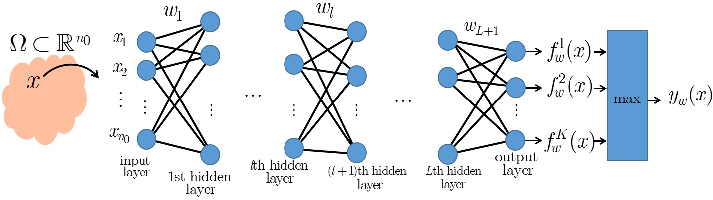
We consider an -hidden-layer DL network, with input domain and output space , whose purpose is to classify a given test data point into one of target classes; here we focus on the supervised learning case so that is known in advance. At the -th layer, (the th layer is the output layer), the output from the -th layer is mapped into according to
| (1) |
in which and are, respectively, the weight matrix and the bias vector, and is the element-wise activation function, each one assumed to be continuous and strictly increasing. Towards a compact description of the network, we stack the weight and bias of the -th layer into
| (2) |
concatenated one next to another to obtain the network parameter vector
| (3) |
In the sequel we denote by the collection of all network parameter vectors. The input-output relation of a DL network, represented by , can be described by a continuous function as
| (4) |
which is a composition of the mapping (1) layer after layer. Let be the th component of , and the label of the data point predicted by . Then we have
| (5) |
If is not a singleton, the network makes a random guess among the reported indexes. A schematic summary of the network model for data classification is given in Fig. 3. The following assumption is made throughput the paper.
Assumption 1.
The input domain is endowed with a probability measure so that is a probability space, where the event space is a sigma algebra of sunsets of , and the probability measure of is denoted by .
III Proposed distance measure
III-A Formulation
Construction of our proposed distance measure is built on an equivalent characterization of the decision rule (5). For definiteness, we decompose the output space into
| (6) |
in which
| (7) |
and is the union of boundaries between ’s. Clearly, the network predicts for a unique label, say, , once ; otherwise, i.e., , whenever . Therefore, the input subset of over which is
| (8) |
where stands for the inverse image of under ; all those with then belong to . The core idea behind is: If two networks and perform close, the event “ differs from throughout ” is of a small probability. To formalize matters, we consider the symmetric difference [51] between and , namely,
| Truncated Gaussian | 0.8513 | 0.1395 | 0.8482 |
|---|---|---|---|
| Uniform | 0.9118 | 0.0828 | 0.9196 |
| (9) |
and then propose the following distance measure
| (10) |
where the scalar is included as a normalization factor. For the three network parameter vectors in Table I, we compare in Table II their for input data sampled from the square region according to the truncated Gaussian (zero-mean and unit variance) and uniform distributions, respectively. The results show that is large, accounting for their drastically different classification outcomes seen in Fig 2, and is small, well justifying and perform close. This example bespeaks that, compared to the Euclidean metric (see Table I), our distance measure (10) can better discriminate networks according to their classification outcomes.
III-B Properties of
The distance measure (10) enjoys an appealing property, stated below.
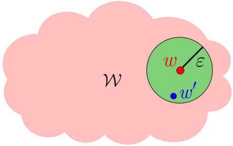
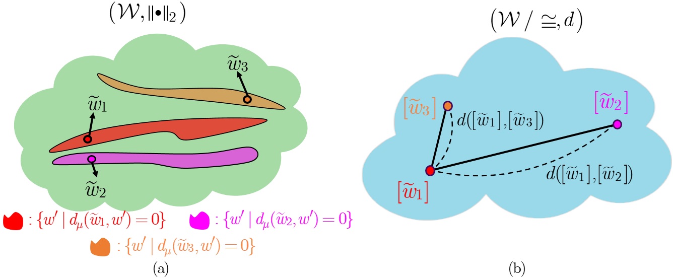
Hence, gauges how likely the decisions of and disagree. In particular, if is the ground truth classifier, is exactly the generalization error [8, 9] achieved by . In view of this, a network admitting a generalization error less than lies in the -neighborhood centered at the ground truth , as illustrated in Fig. 4. With such a nice geometry in mind, we embark on investigating the mathematical structure behind , say, if it is a metric [15, 16] over .
From (3.5), is for sure non-negative; also, it is symmetric and satisfies the triangular inequality, as asserted below.
However, it is easy to see from (10) that , i.e., the event “ agrees with ” is of zero probability, does not guarantee , meaning that is not a metric. Fortunately, the story does not just end here, as we elaborate more next.
IV Metric topology
IV-A Metric topology on quotient set of
We observe that defines an equivalent relation, hereafter denoted by , on . Indeed, reflexivity, i.e., , , and symmetry, i.e., implies , follow immediately from definition (10). Transitivity, that is, leads to , is a direct consequence of the triangular inequality in Property 2 (b). For , let
| (12) |
be the class consisting of all elements equivalent to , that is to say, of those networks performing as good as when judged according to the proposed distance measure (10). In (12), is the representation of the class. We then consider the quotient set of modulus the equivalent relation , namely,
| (13) |
Notably, the union of all equivalent classes in forms a disjoint partition of [19]. We prefer to because, in , each is deemed as a “point” to facilitate analyses (say, of performance gaps between distinct classes) on an elegant point-wise basis. On we go on to define by
| (14) |
in order to evaluate the distance between two equivalent classes . From (10) and (14), it is worthy of noting , which is exactly the distance between the representations and of the two classes. Even though is not a metric on , things are totally different if we instead look at the quotient set in conjunction with . To be specific, the next theorem holds.
Theorem IV.1.
The distance measure in (14) is a metric on the quotient set .
Proof.
Non-negativity, symmetry, and the triangle inequality hold immediately by using Property 2. It thus remains to prove if and only if . Assuming , we must have , implying . Conversely, if , then and yield different classification performances so that . The proof is completed. ∎
Hence, is a metric space of all equivalent classes of , each one composed of networks performing equally well. The distinctive features of our proposal are three-fold. First, while networks performing equally well are “spread over” when viewed from the Euclidean metric, they are identified as an equivalent class, thus a unity as a whole, under the proposed equivalent relation. Second, the endowed metric on the associated quotient set allows us to accurately assess the performance gap between distinct classes on a point-wise basis (see Fig. 5 for an illustration). Third, capitalized on the rich metric space theory, we stand to investigate some important properties about ; this is done in the next Section. Before that, we revisit the foregoing toy example in Introduction to illustrate the proposed metric topology.
IV-B Example
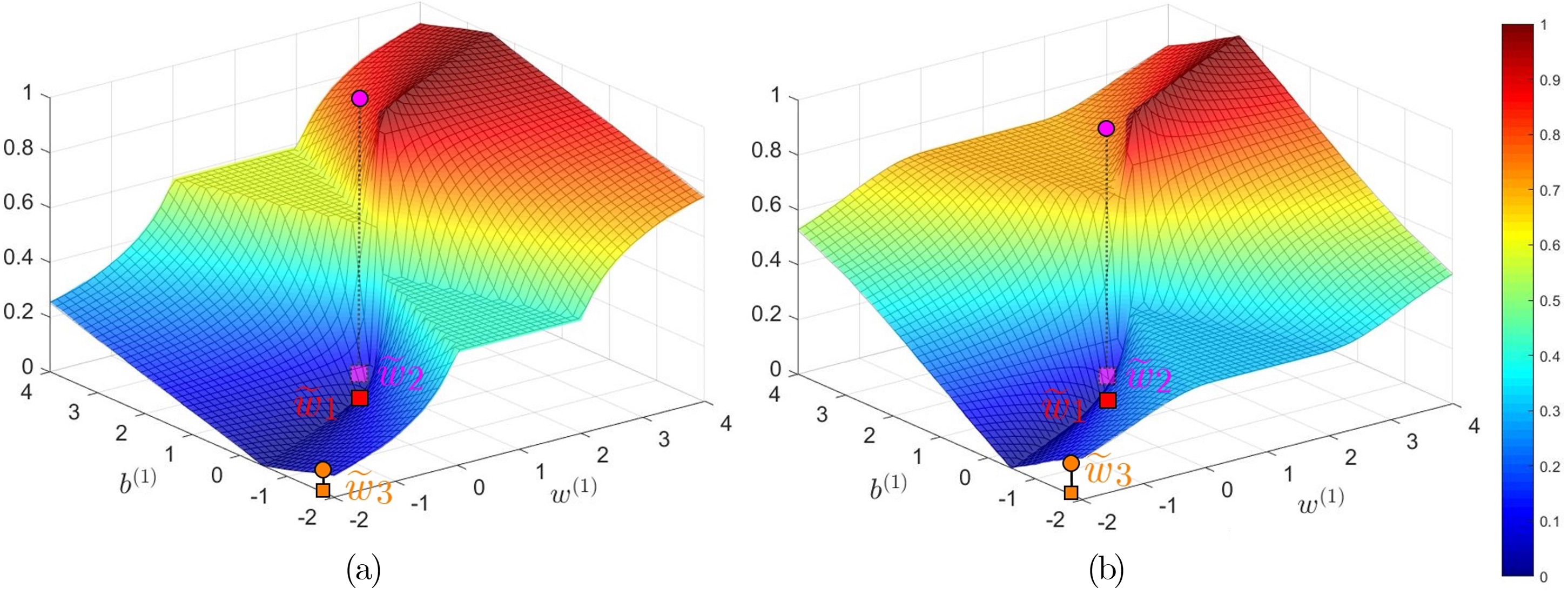
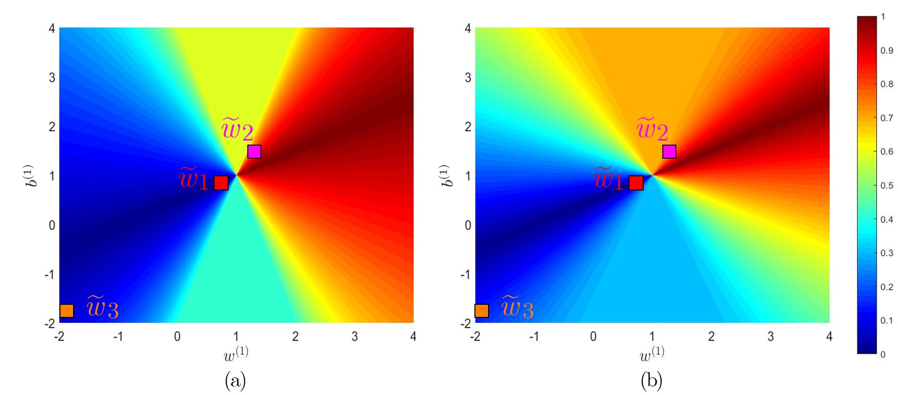
For the one-layer DL network with six real parameters shown in Fig. 1, it is impossible to directly depict the equivalent classes in the network parameter vector space . To ease illustration, we simply set so that only and remain free parameters; that is, we just look at the projections onto the two-dimensional -plane subject to the designated equality constraints. For given in Table I, Fig. 6-(a) and Fig. 6-(b) plot the computed with respect to the pairs ; the input data, drawn from , obey the two distributions considered above. In both figures, the pairs achieving zero distance (the darkest color) belong to . Notably, there is a sharp change in around . Actually, further zooming in on the plot shows the existence of a discontinuity at , which corresponds to the network parameter vector . Such an “all-one” network results in identical network outputs ( in Fig. 1), then making a random guess between the two indexes. Here, a pair other than represents a network certain to predict a unique label. Consequently, the vicinity of abounds in such “normal” networks from different equivalent classes, one with different distance : this accounts for the drastic change in around . A rigorous study of this phenomenon is addressed in the next section. To better visualize the “projected” equivalent classes, Fig. 7-(a) and Fig. 7-(b) plot the “bird’s eye view” of the level surfaces in Fig. 6-(a) and Fig. 6-(b), respectively. The pairs in the same equivalent class (of the same color) are seen to form a ray emanating from . The figures also clearly show the discontinuity is surrounded by elements from distinct equivalent classes.
V Theoretical results
Now we are in a position to state the main theoretical results of this paper. The analyses throughout are built on the following assumptions.
Assumption 2.
The input domain is bounded, say,
| (15) |
for some finite .
Assumption 3.
The set of network parameter vectors is bounded, i.e.,
| (16) |
for some finite .
Boundedness of the input domain is valid since practical data samples are of finite power; so is the boundedness of because real-world implementations prevent unlimited growth in the total network power. Without loss of generality, we therefore identify the input domain , and the network weight set as well, with a bounded and closed Euclidean two-norm ball so that both and are compact in the Euclidean metric; such a property can facilitate our on-going analytic study. Alongside the boundedness assumptions, the following condition to balance the probability measure of event subsets is required.
Assumption 4.
The probability measure of each event satisfies for some .
Assumption 4 excludes impulse-type probability densities; hence small (in Lebesgue measure) events are rare and, in particular, measure-zero events never occur. Such a requirement is fulfilled by many practical data distributions. Indeed, for the input domain in (15), we have , where being the Euler’s Gamma function [52], for the uniform distribution, and for the truncated Gaussian distribution with zero mean and identity covariance matrix.
V-A Projection map
In regards to equivalent relation and the associated quotient set, the projection map [19], specifically in our case defined by
| (17) |
is rather pivotal. Here we stress that is a mapping between two metric spaces, from the Euclidean into the quotient set endowed with the proposed metric (14). To proceed, we first recall from Section III-A that, for a given , is the associated input subset such that . If , the network then has a chance to predict for -distributed data non-unique labels. The set of such networks is virtually nil in the domain of , as asserted by the following theorem.
Theorem V.1.
Proof.
See Appendix C. ∎
On account of Theorem V.1, networks certain to predict for -distributed data a unique label are almost everywhere in . In the example given in Section IV-B, is a singleton of the all-one vector , corresponding to in the Fig. 6 and 7; it is clearly of Lebesgue measure zero. The projection map in (17) enjoys the following nice property.
Proof.
See Appendix D. ∎
Discontinuities of on the subset is not unexpected. This is because, for , hence , there exists in every its neighborhood a , with , such that is bounded from below by a small factor of , no matter how close and are. As an illustration using the example in Section IV-B, the discontinuity occurs at , aside from which the distance varies smoothly. Continuity of specified by the above theorem will be exploited to devise two important properties regarding the proposed metric topology, as done next.
V-B Properties of metric topology
First of all, we note that a subset of Lebesgue measure zero warrants the existence of an arbitrarily small open cover [15]. Therefore, given there exists an Euclidean open with such that . From now on we will call an -pruned network set, to retain all networks in except those in a “vanishingly small” open cover of . When restricted to , the resultant quotient set endowed with the proposed metric topology is compact. More precisely we have the following.
Theorem V.3.
In the literature of topological space, one natural and widely-considered topology on the quotient set modulo the equivalent relation is the quotient topology [19], which is the collection of all subsets such that the inverse image under the projection map is open in . The following theorem asserts that, if we choose to stay in , our proposed metric topology on coincides with the quotient topology.
Theorem V.4.
Under Assumptions 14, and given an -pruned , the collection of all open subsets in the metric space is the quotient topology on .
Proof.
It suffices to show that
-
(a)
For any , i.e., is open in , the inverse image is open in .
-
(b)
If is an open subset such that for some , then lies in .
Part (a) is clearly true thanks to the continuity of the projection shown in Theorem V.2. We then go on to prove part (b). Since is a closed subset of a bounded set in the Euclidean space, by the Heine–Borel theorem [16] is compact. Since the projection is continuous, is compact [15, Theorem 4.2.2] in . Since every compact set in a metric space is closed [15, p.174], is open in . The proof is thus completed. ∎
VI Summary and discussions
The less than tractable nonlinearity and layered architecture have posed a big challenge for theoretical analyses and study of DL. While researchers have raced for developing mathematical foundations of DL, current achievements would seem far from complete and unified. So new mathematical elements able to gain further insights into DL are definitely important and welcome. This paper presents some of our findings through the lens of metric topology, a fundamental and well-established tool in mathematical analysis yet still absent from the DL literature. We first propose a probabilistic-based distance measure, as a replacement of conventional Euclidean metric, to assess the performance gap between two networks according to their classification performances. This distance measure is reminiscent of the thread in statistical learning theory, specialized to the well-known generalization error of a network when compared against the ground truth classifier. Although not a metric among network parameter vectors, it defines an equivalent relation able to identify networks performing equally well with one single equivalent class. Our distance measure then provably serves as a metric on the quotient set modulo the equivalent relation. Under quite mild conditions, we go on to present a series of analyses into the proposed metric space. Continuity of the projection map, except for a Lebesgue measure zero subset of networks likely to mark ambiguous labels, is first established. Aided by this result, two important properties regarding our metric topology, namely, compactness and equivalence to the well-known quotient topology, are then established.
Our study opens up several interesting future research directions. First and foremost, how the proposed quotient set and metric space formulation can shed light on algorithmic design is of high interest. Since compactness implies completeness, one possible approach is devising new design objectives that are contraction [15, 16]; the celebrated Banach contraction mapping principle [53, 54] along with simple fixed-point iteration then offers a potential framework for algorithm design. Of further topological aspects yet to be explored is connectivity, an enabling property for developing algorithms on the basis of algebraic topology [55, 56, 57]. Although the metric topology proposed in this work is specifically constructed and applied to data classification problems, it can be extended to deal with DL-empowered regression and multi-armed bandit problems [58, 59] according to our preliminary investigation.
Appendix A Proof of Property 1
Appendix B Proof of Property 2
Part (a) holds directly holds from (9) and (10) since
| (20) | ||||
To prove part (b), let , therefore either or . For the case that , either or , which implies that
| (21) |
Similar to (21), for the case that we have
| (22) |
With (21) and (22), it follows that
| (23) | ||||
which in conjunction with the subadditivity of measure yields
| (24) | ||||
The proof is thus completed.
Appendix C Proof of Theorem V.1
By the definition (8), we have
| (25) | ||||
where (a) follows directly from the decision rule (5). Using (25) along with the union bound we reach
| (26) | ||||
Hence, once the right-hand-side of (26) is zero, which is true if
| (27) |
Under Assumption 4, a sufficient condition for (27) is
| (28) |
Indeed, supposing (28) is true (the proof of (28) is shown later) we immediately have
| (29) | ||||
where is the indicator function [60, p.68], (a) follows from the Tonelli’s theorem [60, Theorem 6.10], and (b) holds due to (28). Use the Tonelli’s theorem again to rewrite (29) as
| (30) | ||||
Hence, the equality holds almost everywhere in . As a result, we have
| (31) | ||||
Since, from Assumption 4,
| (32) | ||||
it follows
| (33) | ||||
Combining (LABEL:eq:6_7) and (LABEL:eq:6_9) then proves (27).
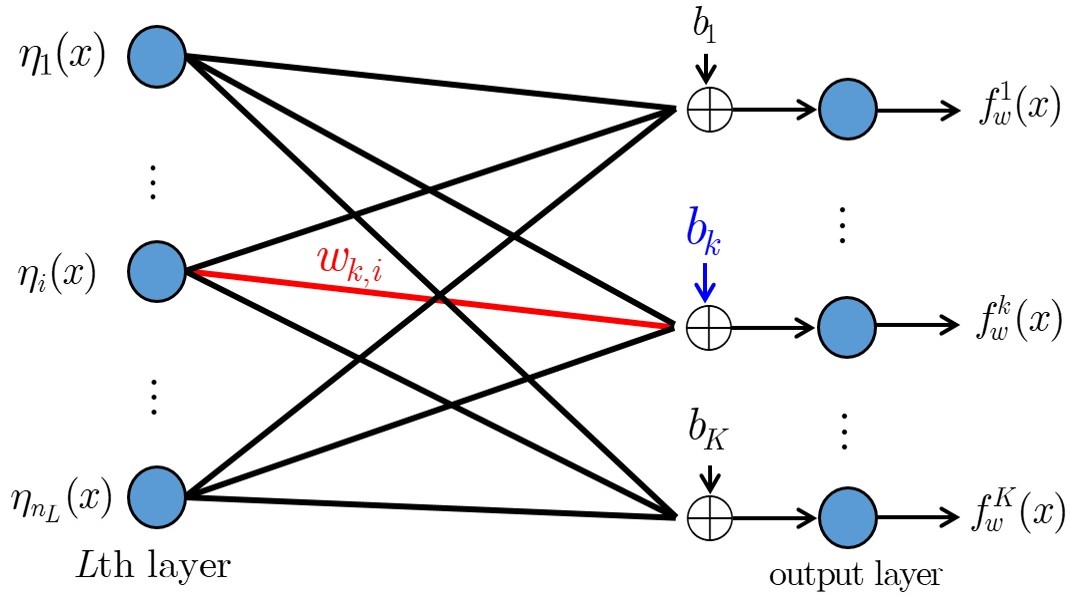
We then go on to prove (28). Towards this end, let be the output of the th node at the th layer, be the weight of the edge connecting the th node at the th layer and the th node at the output layer, and be the bias of the th node at the output layer; see Fig. 8 for an illustration. From (1), a compact representation of is
| (34) |
Since the activation function is strictly increasing, it is clear that if and only if
| (35) |
and therefore
| (36) |
Let us stack all the weight and bias parameters except into . Then we deduce from (36) that
| (37) | ||||
where (a) follows from the Tonelli’s theorem, and (b) holds since a singleton is measure zero in . The proof is thus completed.
Appendix D Proof of Theorem V.2
We first prove that the projection map (17) is continuous on . Let and such that . Our goal is to show as . Note that, since , (18) implies , consequently . Then, using (14), it follows
| (38) | ||||
where (a), (b), and (c) follow from (9), (8), and (7), respectively. Since is compact (under Euclidean metric) and , , are continuous functions, ’s are uniformly continuous [15, Theorem 4.6.2]. This guarantees for each the existence of a such that
| (39) |
If we pick , (39) then implies
| (40) |
In particular, for with , (40) implies
| (41) |
Accordingly, if , (41) then gives , thereby
| (42) |
Using (42), we immediately have
| (43) | ||||
Combining (38) and (LABEL:eq:6_19) yields
| (44) |
On the other hand, since , , is continuous over the input domain , associated with a positive integer the inverse image of under
| (45) |
is (Euclidean) open, thus measurable. Since as and is finite, the Bounded Convergence Theorem (e.g., [60, Theorem 10.11]) implies
| (46) | ||||
where (a) holds by the definition of below (8), and (b) holds due to . Setting on both sides of (44) along with (46) then gives . Thus, we complete the proof that the projection map (17) is continuous on . We then go on to show that the projection map (17) is discontinuous on . Let and . Since is of Lebesgue measure zero, there exists such that and thus . By the definition (14), we have
| (47) | ||||
where (a) holds since . Hence, is lower bounded by , no matter how small is. Hence, the projection map (17) is discontinuous on . The proof is thus completed.
References
- [1] I. Goodfellow, Y. Bengio, and A. Courville, Deep Learning. The MIT Press, 2016.
- [2] C. F. Higham and D. J. Higham, “Deep learning: An introduction to applied mathematicians,” SIAM Reviews, vol. 61, no. 4, pp. 860–891, 2019.
- [3] H. Bolcekei, P. Grohs, G. Kutynoik, and P. Petersen, “Optimal approximation with sparsely connected deep neural networks,” SIAM J. Mathematics of Data Science, vol. 1, no. 1, pp. 8–45, 2019.
- [4] M. Cacciola, A. Frangioni, X. Li, and A. Lodi, “Deep neural networks pruning via the structured perspective regularization,” SIAM J. Mathematics of Data Science, vol. 5, no. 4, pp. 1051–1077, 2023.
- [5] M. Elad, B. Kawar, and G. Vaksman, “Image denoising: The deep learning revolution and beyond,” SIAM J. Image Science, vol. 16, no. 3, pp. 1594–1654, 2023.
- [6] M. Soltanolkotabi, A. Javanmard, and J. D. Lee, “Theoretical insights into the optimization landscape of over-parametered shallow neural networks,” IEEE Trans. Information Theory, vol. 65, no. 2, pp. 742–769, Feb. 2019.
- [7] P. Grohs and G. Kutyniok, Mathematical Aspects of Deep Learning. Cambridge University Press, 2023.
- [8] M. Mohri, A. Rostamizadeh, and A. Talwalkar, Foundations of Machine Learning, 2nd ed. The MIT Press, 2018.
- [9] S. S. Shwartz and S. B. David, Understanding Machine Learning: From Theory to Algorithms. Cambridge University Press, 2014.
- [10] T. Wiatowski and H. Bolcskei, “A mathematical theory for deep conventional neural networks for feature extraction,” IEEE Trans. Information Theory, vol. 64, no. 3, pp. 1845–1866, 2018.
- [11] V. Dunjko and H. J. Briegel, “Machine learning and artificial intelligence in the quantum domain: a review of recent progress,” Reports on Progress in Physics, vol. 81, no. 7, 2018.
- [12] M. R. Hush, “Machine learning for quantum physics,” Science, vol. 355, no. 6325, p. 580, 2017.
- [13] M. Schuld, I. sinayskiy, and F. Petruccione, “An introduction to quantum machine learning,” Contemporary Physics, vol. 56, no. 2, pp. 172–185, 2015.
- [14] J. Heinonen, Lectures on Analysis on Metric Spaces. Springer, 2001.
- [15] J. E. Marsden and M. J. Hoffman, Elementary Classical Analysis. W. H. Freeman Co, 1993.
- [16] W. Rudin, Principles of Mathematical Analysis, 3rd ed. McGraw-Hill Education, 2023.
- [17] O. Bousquet and A. Elisseeff, “Stability and generalization,” J. Machine Learning Research, vol. 2, pp. 499–526, 2002.
- [18] C. Zhang, S. Bengio, M. Hardt, B. Recht, and O. Vinyals, “Understanding deep learning (still) requires rethinking generalization,” Communications of the ACM, vol. 63, no. 3, pp. 107–115, 2021.
- [19] T. W. Gamelin and R. E. Greene, Introduction to Topology, 2nd ed. Dover Publications. Inc., 1999.
- [20] J. R. Munkres, Topology, 2nd ed. Prentice Hall, Inc., 2000.
- [21] P. Bendich, J. S. Marron, E. Miller, A. Pieloch, and S. Skwerer, “Persistent homology analysis of brain artery trees,” The Annals of Applied Statistics, vol. 10, no. 1, pp. 198–218, 2016.
- [22] H. Lee, M. K. Chung, H. Kang, B. N. Kim, and D. S. Lee, “Discriminative persistent homology of brain networks,” IEEE International Symposium on Biomedical Imaging, pp. 841–844, 2011.
- [23] G. Singh, F. Memoli, and G. Carlsson, “Topological methods for the analysis of high dimensional data sets and 3d object recognition,” Eurographics Symposium on Point-Based Graphics, pp. 91–100, 2007.
- [24] H. Wu, A. Yip, J. Long, J. Zhang, and M. K. Ng, “Simplicial complex neural networks,” IEEE Trans. on Pattern Analysis and Machine Intelligence, vol. 46, no. 1, pp. 561–575, 2024.
- [25] G. Carlsson, “Topology and data,” Bulletin of the American Mathematical Society, vol. 46, no. 2, pp. 255–308, 2009.
- [26] H. Krim, T. Gentimis, and H. Chintakunta, “Discovering the whole by the coarse,” IEEE Signal Processing Magazines, vol. 33, no. 2, pp. 95–104, 2016.
- [27] X. G. Xia, “Small data, mid data, and big data versus algebra, analysis, and topology,” IEEE Signal Processing Magazines, vol. 34, no. 1, pp. 48–51, Jan. 2017.
- [28] H. Adams, T. Emerson, M. Kirby, R. Neville, C. Peterson, and P. Shipman, “Persistence images: A stable vector representation of persistent homology,” J. Machine Learning Research, vol. 18, no. 8, pp. 1–35, 2017.
- [29] P. Bubenik, “Statistical topological data analysis using persistence landscapes,” J. Machine Learning Research, vol. 16, no. 1, pp. 77–102, 2015.
- [30] G. Naitzat, A. Zhitnikov, and L. H. Lim, “Topology of deep neural networks,” J. Machine Learning Research, vol. 21, pp. 1–40, 2020.
- [31] M. Gabella, “Topology of learning in feedforward neural networks,” IEEE Trans. on Neural Networks and Learning Systems, vol. 32, no. 8, pp. 3588–3592, 2021.
- [32] M. Gidea, D. Goldsmith, Y. Katz, P. Roldan, and Y. Shmalo, “Topological recognition of critical transitions in time series of cryptocurrencies,” Physica A: Statistical mechanics and its applications, vol. 548, 2020.
- [33] Y. Hiraoka, T. Nakamura, A. Hirata, E. G. Escolar, K. Matsue, and Y. Nishiura, “Hierarchical structures of amorphous solids characterized by persistent homology,” Proceedings of the National Academy of Sciences, vol. 113, no. 26, pp. 7035–7040, 2016.
- [34] C. Hofer, R. Kwitt, M. Niethammer, and A. Uhl, “Deep learning with topological signatures,” in Proceedings of the 31st Conference of Neural Information Processing Systems, 2017.
- [35] V. Carrière, M. Cuturi, and S. Oudot, “Sliced wasserstein kernel for persistence diagrams,” in Proceedings of the 34th International Conference on Machine Learning, PMLR, vol. 70, 2017, pp. 664–673.
- [36] J. Reininghaus, S. Huber, U. Bauer, and R. Kwitt, “A stable multi-scale kernel for topological machine learning,” in Proceedings of the IEEE conference on computer vision and pattern recognition, 2015, pp. 4741–4748.
- [37] C. Hofer, R. Kwitt, M. Niethammer, and M. Dixit, “Connectivity-optimized representation learning via persistent homology,” Proceedings of Machine Learning Research, 2019.
- [38] S. Gholizadeh, A. Seyeditabari, and W. Zadrozny, “Topological signature of 19th century novelists: Persistent homology in text mining,” Big Data and Cognitive Computing, vol. 2, no. 4, 2018.
- [39] J. R. Clough, N. Byrne, I. Oksuz, V. A. Zimmer, J. A. Schnabel, and A. P. King, “A topological loss function for deep-learning based image segmentation using persistent homology,” IEEE Trans. on Pattern Analysis and Machine Intelligence, vol. 44, no. 12, pp. 8766–8778, Dec. 2022.
- [40] X. Hu, F. Li, D. Samaras, and C. Chen, “Topology-preserving deep image segmentation,” Advances in Neural Information Processing Systems 32, 2019.
- [41] E. R. Love, “Topological convolutional layers for deep learning,” J. Machine Learning Research, vol. 24, no. 59, pp. 1–35, 2023.
- [42] C. Chen, X. Ni, Q. Bai, and Y. Wang, “A topological regularizer for classifiers via persistent homology,” in Proceedings of the 22th International Conference on Machine Learning, PMLR, vol. 89, 2019, pp. 2573–2582.
- [43] R. Deng and f. Duzhin, “Topological data analysis helps to improve accuracy of deep learning models for fake news detection trained on very small training sets,” Big Data and Cognitive Computing, vol. 6, no. 3, 2022.
- [44] M. E. Aktas, E. Akbas, and A. E. Fatmaoui, “Persistence homology of networks: methods and applications,” Applied Network Science, vol. 4, no. 1, pp. 1–28, 2019.
- [45] S. Barbarossa and S. Sardellitti, “Topological signal processing: Making sense of data building on multiway relations,” IEEE Signal Processing Magazines, vol. 37, no. 6, pp. 174–183, Nov. 2020.
- [46] N. Otter, M. A. porter, U. Tillmann, P. Grindrod, and H. A. Harrington, “A roadmap for the computation of persistent homology,” EPJ Data Science, vol. 6, pp. 1–38, 2017.
- [47] H. Edelsbrunner and J. L. Harer, Computational Topology: An Introduction. American Mathematical Society, 2022.
- [48] L. Wasserman, “Topological data analysis,” Annual Review of Statistics and Its Application, vol. 5, no. 1, pp. 501–532, 2018.
- [49] A. Zia, A. Khamis, J. Nichols, U. B. Tayab, Z. Hayder, V. Rolland, E. Stone, and L. Petersson, “Topological deep learning: a review of an emerging paradigm,” Artificial Intelligence Review, vol. 57, no. 77, 2024.
- [50] H. D. Macedo and J. N. Oliveira, “Typing linear algebra: A biproduct-oriented approach,” Science of Computer Programming, vol. 78, no. 11, pp. 2160–2191, 2013.
- [51] V. I. Bogachev, Measure Theory. Springer, 2007.
- [52] S. Li, “Concise formulas for the area and volume of a hyperspherical cap,” Asian Journal of Mathematics Statistics, vol. 4, no. 1, pp. 66–70, 2011.
- [53] P. Agarwal, M. Jleli, and B. Samet, Fixed Point Theory in Metric Spaces: Recent Advances and Applications. Springer, 2018.
- [54] I. Gohberg and S. Goldberg, Basic Operator Theory. Birkhäuser, 1981.
- [55] A. Hatcher, Algebraic topology. Cambridge University Press, 2002.
- [56] E. H. Spanier, Algebraic topology. Springer-Verlag, 1966.
- [57] G. Strang, Linear Algebra and Learning from Data. Wellesley-Cambridge Press, 2019.
- [58] P. Xu, Z. Wen, H. Zhao, and Q. Gu, “Neural contextual bandits with deep representation and shallow exploration,” in International Conference on Learning Representations, 2022.
- [59] T. Zhu, G. Liang, C. Zhu, H. Li, and J. Bi, “An efficient algorithm for deep stochastic contextual bandits,” in Proceedings of the AAAI Conference on Artificial Intelligence, vol. 35, 2021, pp. 11 193–11 201.
- [60] R. L. Wheeden and A. Zygmund, Measure and Integral: An Introduction to Real Analysis, 2nd ed. CRC Press, 2015.