Bounding the Settling Time of Finite-Time Stable Systems using Sum of Squares

Abstract

Finite-time stability (FTS) of a differential equation guarantees that solutions reach a given equilibrium point in finite time, where the time of convergence depends on the initial state of the system. For traditional stability notions such as exponential stability, the convex optimization framework of Sum-of-Squares (SoS) enables the computation of polynomial Lyapunov functions to certify stability. However, finite-time stable systems are characterized by non-Lipschitz, non-polynomial vector fields, rendering standard SoS methods inapplicable. To this end, in this paper, we show that the computation of a non-polynomial Lyapunov function certifying finite-time stability can be reformulated as computation of a polynomial one under a particular transformation that we develop in this work. As a result, SoS can be utilized to compute a Lyapunov function for FTS. This Lyapunov function can then be used to obtain a bound on the settling time. We first present this approach for the scalar case and then extend it to the multivariate case. Numerical examples demonstrate the effectiveness of our approach in both certifying finite-time stability and computing accurate settling time bounds. This work represents the first combination of SoS programming with settling time bounds for finite-time stable systems.

1 Introduction

For nonlinear systems, there exist multiple non-equivalent notions of stability, including: Lyapunov stability, asymptotic stability, exponential stability, and rational stability (See (Khalil, 1991) and (Bacciotti and Rosier, 2005)). However, all of these notions of stability are asymptotic in the sense that none of them imply that solutions of a given system will ever reach a given stable set. By contrast, the notion of finite-time stability of a set, $X$, ensures that for any initial condition, $x$, there exists a time, $T(x)$ such that if $x(t)$ is a solution then $x(t)\in X$ for all $t\geq T(x)$.

Finite-time stability plays a critical role in control applications, such as the design of robust controllers for sliding mode control (SMC) algorithms (Polyakov and Poznyak, 2012; Polyakov and Fridman, 2014). Specifically, in SMC, asymptotic stability is only guaranteed once the solution reaches the sliding surface and hence twisting (Torres-Gonzalez et al., 2017; Levant, 1993) and super-twisting algorithms (Basin and Ramírez, 2014; Seeber et al., 2018; Moreno and Osorio, 2012) are explicitly designed to achieve finite-time convergence to this surface. In addition, continuity of, and bounds on, the settling time function $T(x)$ can be used, e.g. in robotics, to schedule a sequence of predefined motions – each of which presumes some initial pose Galicki (2015); Zhao et al. (2010); Kong et al. (2020). Consequently, there has been significant recent interest in finding methods for determining finite-time stability and establishing bounds on the settling function $T(x)$.

Methods for establishing finite-time stability are typically based on the use of Lyapunov functions and the comparison principle Bhat and Bernstein (2000, 1995, 1998); Haimo (1986); Venkataraman and Gulati (1990); Moulay and Perruquetti (2006). Because finite-time stability of an equilibrium necessarily implies a non-Lipschitz vector field, however, the Lyapunov framework is more nuanced than in the case of asymptotic stability notions and behaviour of the Lyapunov function near the equilibrium results in multiple Lyapunov characterizations (e.g. Lyapunov conditions in Bhat and Bernstein (2000) differ significantly from those in Roxin (1966)). Moreover, although the Lyapunov framework for finite-time stability is relatively well-established, and has been used in an ad hoc manner for particular applications Cortés (2006); Srinivasan et al. (2018); Mendoza-Avila et al. (2017); Seeber et al. (2018); Torres-Gonzalez et al. (2017); Wang and Xiao (2010), this framework has not resulted in algorithms for testing finite-time stability in the same way that Sum of Squares (SoS) is used to test rational stability of polynomial vector fields. The goal of this paper, then, is to establish such an algorithm.

For systems governed by polynomial vector fields, SoS programming, in conjunction with converse Lyapunov theorems, has proven to be an effective tool for stability certification (Topcu et al., 2008; Jarvis-Wloszek et al., 2005). Unfortunately, however, SoS methods are typically limited to analysis of systems with polynomial or rational vector fields and finite-time stable systems are typically characterized by non-polynomial dynamics. Attempts to extend SoS to non-polynomial vector fields include methods such as recasting, wherein the solutions of a non-polynomial system are embedded in a larger state-space with polynomial dynamics (Savageau and Voit, 1987) – to which SoS methods can be applied (Papachristodoulou and Prajna, 2005). However, such methods are conservative in that instability of the recast system does not imply instability of the original system. More significantly, of course, polynomial vector fields cannot be finite-time stable and hence such methods cannot be applied to the construction of finite-time stability tests using SoS.

In this paper, we specifically consider the case of a vector field defined by non-polynomial terms. Then, instead of recasting the dynamics using a polynomial vector field, we take an alternative approach wherein we first pose the problem of finding a Lyapunov function which verifies finite-time stability – Sec. 4. Such a condition includes fractional terms in both the dynamics and Lyapunov function. However, as demonstrated in Sec. 5, a change of variables in the Lyapunov inequalities allows the fractional inequality constraints to be represented by polynomial inequalities and SOS, where we define a map from the solution to polynomials and polynomial/SOS inequalities back to a fractional Lyapunov function which verifies the original stability conditions – Sec. 6. This approach allows us to avoid the conservatism imposed by recasting of the non-polynomial dynamics and results in accurate tests for finite-time stability and accurate bounds on the associated settling time function, $T(x)$. In Sec. 7 we verify the results using several test cases and use numerical simulation to evaluate the resulting bounds on settling time.

2 Notation

$\mathbb{R}^{n}$, $\mathbb{R}_{+}^{n}$, and $\mathbb{N}^{n}$ denote the space of $n$-dimensional vectors of real, positive real, and natural numbers, respectively. $\mathbb{R}[x]$ as the set of real-valued polynomials in variables $x$. The Euclidean norm of a vector $x=[x_{1},\cdots,x_{n}]^{T}\in\mathbb{R}^{n}$ is defined as $\|x\|=\sqrt{x_{1}^{2}+\cdots x_{n}^{2}}$. A neighborhood, $\mathcal{N}$ of a point, $x$ is any set which contains an open set $U$ such that $x\in U\subseteq\mathcal{N}$. The function $\operatorname{sgn}:\mathbb{R}\to\mathbb{R}$ is defined as:

$$\operatorname{sgn}(x)=\begin{cases}\frac{x}{|x|},&\text{if }x\neq 0,\\ 0,&\text{if }x=0.\end{cases}$$

In Thm. 6, we introduce elementwise vector operations for multiplication, $\operatorname{sgn}$ and exponent. Specifically, For $x\in\mathbb{R}^{n}$ and $q\in\mathbb{N}^{n}$, we define the vector $y=x^{q}$ as $y_{i}=x_{i}^{q_{i}}$. We also define vector-valued element-wise $\operatorname{sgn}$ and absolute value functions where if $x\in\mathbb{R}^{n}$ and $y=\operatorname{sgn}(x)$, then $y_{i}=sign(x_{i})$ and if $y=|x|$ then $y_{i}=|x_{i}|$. Finally, we define the element-wise (Hadamard) product of vectors so that if $y=z\cdot x$, then $y_{i}=z_{i}x_{i}$.

3 Sum of Squares Decomposition

In this section, we provide a brief overview of SoS polynomials and how semidefinite programming can be utilized to verify the existence of SoS decomposition. Specifically, a polynomial inequality of the form $p(x)\geq 0$ for all $x\in\mathbb{R}^{n}$ holds if $p$ is a Sum-of-Square polynomial.

Definition 1

A polynomial $p(x)\in\mathbb{R}[x]$ is called a sum of squares (SoS), denoted $p\in\Sigma_{s}$, if there exist polynomials $h_{i}(x)\in\mathbb{R}[x]$ for $i=1,2,\cdots,k$ (where $k\in\mathbb{N}$ ) such that

$$p(x)=\sum^{k}_{i=1}h_{i}(x)^{2}.$$

The existence of a SoS representation of a polynomial, $p$, can be tested using semidefinite programming (Parrilo, 2000). Specifically, $p(x)$ of degree $2d$ is SoS if and only if there exists a positive semidefinite matrix $Q$ such that $p=Z_{d}(x)^{T}QZ_{d}(x)$ where $Z_{d}(x)$ is the vector of monomials in $x$ of degree $d$ or less. In the case where the polynomial inequality is required to hold on a semialgebraic set (i.e. $p(x)\geq 0$ for all $x\in S$), we may use Positivstellensatz results. Specifically, a set $S$ is called semi-algebraic if it can be represented using polynomial equality and inequality constraints as

$$S=\left\{x:\begin{aligned} &g_{i}(x)\geq 0,\quad\forall i=1,\ldots,k,\quad k\in\mathbb{N},\\ &h_{j}(x)=0,\quad\forall j=1,\ldots,m,\quad m\in\mathbb{N}\end{aligned}\right\}.$$

Lemma 2

Given $S=\{x:g_{i}(x)\geq 0,h_{j}(x)=0\}$, suppose there exist $s_{i}\in\Sigma_{s}$ and $t_{j}\in\mathbb{R}[x]$ such that

$$p(x)=s_{0}(x)+\sum^{k}_{i=1}s_{i}(x)g_{i}(x)+\sum^{m}_{j=1}t_{j}(x)h_{j}(x),$$

where $k,m\in\mathbb{N}$. Then $p(x)\geq 0$ for all $x\in S$.

Necessity of this Positivstellensatz test in the case of strictly positive polynomials holds if $s_{i},h_{i}$ satisify an additional precompactness condition (Putinar, 1993, Lemma 4.1). All semialgebraic sets used in this paper satisfy this condition.

4 Problem Formulation

In this paper, we consider the class of nonlinear differential equations of the form

$$\frac{d}{dt}x(t)=f(x(t)),\quad x(0)=x_{0},\quad t\in[0,T),\quad T\in\mathbb{R}_{+},$$ (1)

where $x(t)\in\mathcal{D}\subseteq\mathbb{R}^{n}$ with $\mathcal{D}$ containing an open neighborhood of the origin. Furthermore, we suppose $f:\mathcal{D}\mapsto\mathbb{R}^{n}$ is continuous on $\mathcal{D}$ with $f(0)=0$. However, we do not require $f$ to be locally Lipschitz at the origin. For this reason, we require existence and uniqueness of solutions except possibly at the origin, where such uniqueness is as defined in (Bhat and Bernstein, 2000). In this case, we denote by $\phi:[0,T)\times\mathcal{D}\backslash\{0\}\mapsto\mathcal{D}\backslash\{0\}$ the corresponding solution map for which

$$\frac{d}{dt}\phi(t,x)=f(\phi(t,x)),\quad \forall x\in\mathcal{D}\backslash\{0\},t\in[0,T),$$

$$\phi(0,x)=x,\quad \forall x\in\mathcal{D}\backslash\{0\}.$$

For a nonlinear system with the associated solution map, we may define a notion of finite-time stability using the framework proposed in (Bhat and Bernstein, 2000).

Definition 3

Given $f$ and $\mathcal{O}\subset\mathcal{D}$ containing an open neighborhood of the origin, we say the solution map $\phi:[0,T)\times\mathcal{D}\backslash\{0\}\mapsto\mathcal{D}\backslash\{0\}$ is finite-time stable on $\mathcal{O}$ with settling time function $T:\mathcal{O}\backslash\{0\}\rightarrow\mathbb{R}_{+}$ if it is stable in the sense of Lyapunov and for every $x\in\mathcal{O}\backslash\{0\}$, $\phi(t,x)\in\mathcal{O}\backslash\{0\}$ for all $t\in[0,T(x))$ and $\lim_{t\to T(x)}\phi(t,x)=0.$ If $\mathcal{O}=\mathcal{D}=\mathbb{R}^{n}$, we say that $\phi$ is globally finite-time stable.

While the above definition of finite-time stability allows for any valid settling time function, to avoid ambiguity, henceforth we refer to “the settling time function” as the function, $T$, which is defined as $T(0)=0$ and $T(x)=\inf\{t\in\mathbb{R}_{+}\mid\phi(t,x)=0\}.$ The goal of this paper, is to prove finite-time stability of systems with fractional dynamics and to obtain least upper bounds on the associated settling time function. To achieve this goal, we rely on the Lyapunov characterization of finite-time stability and the associate settling time function developed in (Bhat and Bernstein, 2000, Theorem 4.2):

Theorem 4

Suppose there exists a continous function $V:\mathcal{D}\mapsto\mathbb{R}$ such that the following conditions hold:

1. $V$ is positive definite.

2. There exist real numbers $\mu$ and $\gamma\in(0,1)$ and an open neighborhood $\Omega\subseteq\mathcal{D}$ of the origin such that

   $$\dot{V}(x)+\mu V(x)^{\gamma}\leq 0,\quad x\in\Omega\backslash\{0\}.$$ (2)

Then the solution map $\phi_{f}:[0,T)\times\mathcal{D}\backslash\{0\}\rightarrow\mathcal{D}\backslash\{0\}$ of (1) is finite-time stable. Moreover, if $\mathcal{O}$ is contained in a sublevel set of $V$ contained in $\Omega$ and $T$ is the settling-time function, then

$$T(x)\leq\frac{1}{\mu(1-\gamma)}V(x)^{1-\gamma},\quad x\in\mathcal{O},$$ (3)

and $T$ is continuous on $\mathcal{O}$. If in addition $\mathcal{D}=\mathbb{R}^{n},V$ is proper, and $\dot{V}$ takes negative values on $\mathbb{R}^{n}\backslash\{0\},$ then the origin is a globally finite-time-stable equilibrium of (1).

While Thm. 4 provides sufficient conditions for finite-time stability in terms of a continuous Lyapunov function, these conditions are expressed using a fractional exponent, $\gamma\in(0,1)$. Furthermore, finite time stable systems are defined by non-polynomial vector fields – often containing fractional exponents. As such, typical SoS and polynomial programming methods cannot be applied. In the following section, we show how to reformulate the conditions of Thm. 4 using polynomials and polynomial inequalities.

5 A Polynomial Reformulation of the Finite-Time Stability Problem

The Lyapunov conditions in Thm. 4 contain fractional exponents (e.g. $\dot{V}\leq-V^{1/2}$) and finite-time stable systems typically include vector fields with fractional exponents (e.g. $\dot{x}=-x^{1/5}$). Such fractional terms prevent a straightforward application of polynomial optimization and SoS. In this section, we show how the conditions of Thm. 4 may be enforced without the use of fractional exponents.

To keep the exposition clear, we first state and prove the result for the scalar case, where $f:\mathbb{R}\rightarrow\mathbb{R}$. Building on the scalar case, we provide a similar result for the multivariate case in Thm. 6 later in the paper.

Theorem 5

Let $\mathcal{D}\subseteq\mathbb{R}$ and $f:\mathcal{D}\mapsto\mathbb{R}$ be continuous. Suppose for some $\Omega\subset\mathbb{R}$ there exist a continuously differentiable $V:\Omega\rightarrow\mathbb{R}$, positive constants $\mu,k$, and integers $p,q,r\in\mathbb{N}$ such that $V(0)=0,V(x)>0$ for any $x\in\Omega\backslash\{0\}$, $V(x)\leq k|x|^{r}$ for $x\in\Omega$ , and

$$\nabla_{x}V(x)f(\operatorname{sgn}(x)|x|^{q})\leq-\mu|x|^{p},\quad\forall x\in\Omega.$$ (4)

Let $\tilde{\Omega}:=\{z\in\mathcal{D}:\operatorname{sgn}(z)|z|^{1/q}\in\Omega\}$, $\gamma=\frac{1+p-q}{r}\in\mathbb{R}_{+}$ and $\tilde{\mu}=\frac{\mu}{qk^{\gamma}}$. Then there exists a continuously differentiable $\tilde{V}:\tilde{\Omega}\rightarrow\mathbb{R}$ such that $\tilde{V}(0)=0,\tilde{V}(z)>0$ for any $z\in\tilde{\Omega}\backslash\{0\}$, and

$$\nabla_{z}\tilde{V}(z)f(z)\leq-\tilde{\mu}\tilde{V}(z)^{\gamma},\quad\forall z\in\tilde{\Omega}.$$ (5)

For $z\in\tilde{\Omega}$, define

$$\tilde{V}(z)=V(\operatorname{sgn}(z)|z|^{1/q}).$$

First, $\tilde{V}(0)=V(0)=0$. Next, for any $z\in\tilde{\Omega},$ $\operatorname{sgn}(z)|z|^{1/q}\in\Omega$ and hence $\tilde{V}$ is well-defined on $\tilde{\Omega}$. Furthermore, $\tilde{V}(z)=V(\operatorname{sgn}(z)|z|^{1/q})>0$ for all $z\in\tilde{\Omega}.$

Next, since $V$ is continuously differentiable on $\Omega$ and

$$\frac{\partial}{\partial z}\operatorname{sgn}(z)|z|^{1/q}=\frac{\partial}{\partial z}\operatorname{sgn}(z)\frac{|z|}{|z|}|z|^{1/q}=\frac{\partial}{\partial z}z|z|^{1/q-1}$$

$$=|z|^{1/q-1}+\frac{1-q}{q}z|z|^{1/q-2}\operatorname{sgn}(z)$$

$$=|z|^{1/q-1}+\frac{1-q}{q}|z||z|^{1/q-2}=|z|^{1/q-1}+\frac{1-q}{q}|z|^{1/q-1}$$

$$=\left(1+\frac{1-q}{q}\right)|z|^{1/q-1}=\frac{1}{q}|z|^{1/q-1}$$

is continuous on $\tilde{\Omega}\backslash\{0\}$ (with left and right hand limits agreeing at $z=0$), we have that $\tilde{V}(z)=V(\operatorname{sgn}(z)|z|^{1/q})$ is continuously differentiable on $\tilde{\Omega}$.

Finally, using the chain rule and the expression for
$\frac{\partial}{\partial z}\operatorname{sgn}(z)|z|^{1/q}$, we have:

$$\nabla_{z}\tilde{V}(z)=\nabla_{x}V(\operatorname{sgn}(z)|z|^{1/q})\frac{1}{q}|z|^{1/q-1}.$$

We now observe that

$$\operatorname{sgn}(\operatorname{sgn}(z)|z|^{1/q})|\operatorname{sgn}(z)|z|^{1/q}|^{q}=\operatorname{sgn}(z)|z|=z$$

and hence for $z\in\Omega$, (4) implies

$$\nabla_{x}V(x)|_{x=\operatorname{sgn}(z)|z|^{1/q}}f(z)\leq-\mu|\operatorname{sgn}(z)|z|^{1/q}|^{p}=-\mu|z|^{p/q}.$$

Thus

$$\nabla_{z}\tilde{V}(z)f(z) =\nabla_{x}V(x)|_{x=\operatorname{sgn}(z)|z|^{1/q}}\frac{1}{q}|z|^{1/q-1}f(z)$$

$$\leq-\mu\frac{1}{q}|z|^{1/q-1}|z|^{p/q}=-\frac{\mu}{q}|z|^{\frac{1+p-q}{q}}.$$

However, we know that $V(x)\leq k|x|^{r}$ with $r=\frac{1+p-q}{\gamma}$ which implies

$$\tilde{V}(z)=V(\operatorname{sgn}(z)|z|^{1/q}) \leq k|\operatorname{sgn}(z)|z|^{1/q}|^{\frac{1+p-q}{\gamma}}$$

$$=k|z|^{\frac{1+p-q}{q\gamma}}.$$

Rasing both sides to the power of $\gamma$, we have:

$$\tilde{V}(z)^{\gamma}\leq k^{\gamma}|z|^{\frac{1+p-q}{q}}.$$

Hence, for any $z\in\tilde{\Omega}$ we obtain:

$$\nabla_{z}\tilde{V}(z)f(z)\leq-\frac{\mu}{q}|z|^{\frac{1+p-q}{q}}\leq-\frac{\mu}{qk^{\gamma}}\tilde{V}(z)^{\gamma}$$

as desired. Theorem 5 provides alternative conditions under which Theorem 4 can be used to prove finite-time stability and bound the settling time function. If the vector field, $f$ contains fractional exponents, e.g. $f(x)=-\operatorname{sgn}(x)|x|^{1/2}-x^{1/3}$ then by choosing $q$ to be the least common denominator of these fractional terms, $f(\operatorname{sgn}(z)|z|^{q})$ the fractional terms are eliminated – e.g. $f(\operatorname{sgn}(z)|z|^{6})=-x^{3}-x|x|$. While these alternative conditions are not entirely polynomial, they can then be tested using polynomial optimization as described in Section 6 and illustrated in Section 7 (Example 9). For the multivariate case, however, the conditions are slightly more involved, as seen in the following subsection.

5.1 Finite-Time Stability Conditions for Multivariate
Vector Fields

In Theorem 5 we have shown, in the scalar case, how fractional terms in the Lyapunov test for finite-time stability may be eliminated by a power substitution $x\mapsto\operatorname{sgn}(z)|z|^{q}$. In the multivariate case, we now present similar conditions, although in this case, we allow for multiple variable mappings – e.g. $x_{1}\mapsto\operatorname{sgn}(z_{1})|z_{1}|^{2}$ and $x_{2}\mapsto\operatorname{sgn}(z_{2})|z_{2}|^{6}$. As a result, however, there is an additional step in modifying the vector field so as to allow for a homogeneous bound on the derivative of the Lyapunov function – i.e. the conditions are expressed in terms of a modified vector field $\tilde{f}_{i}(z):=\frac{1}{q_{i}}f_{i}(z)|z_{i}|^{1/q_{i}-1}$.

Theorem 6

Let $\mathcal{D}\subseteq\mathbb{R}^{n}$ and $f:\mathcal{D}\mapsto\mathbb{R}^{n}$ be continuous. Suppose for some $\Omega\subset\mathbb{R}^{n}$ there exist a continuously differentiable $V:\Omega\rightarrow\mathbb{R}$, a vector $q\in\mathbb{N}^{n}$, and scalars $p,\mu,k,r\in\mathbb{R}_{+}$ such that $V(0)=0$, $V(x)>0\quad\text{for any }x\in\Omega\backslash\{0\}$, and $V(x)\leq k\lVert{x}\rVert^{r}$ for $x\in\Omega$. Moreover, suppose

$$\nabla_{x}V(x)^{T}\tilde{f}(\operatorname{sgn}(x)\cdot|x|^{q})\leq-\mu\lVert{x}\rVert^{p},\quad\forall x\in\Omega,$$ (6)

where $\tilde{f}_{i}(z):=\frac{1}{q_{i}}f_{i}(z)|z_{i}|^{1/q_{i}-1}$.

Let $\tilde{\Omega}=\{z\in\mathcal{D}:\operatorname{sgn}(z)\cdot|z|^{1/q}\in\Omega\}$, $\gamma=\frac{p}{r}$, and $\tilde{\mu}=\frac{\mu}{k}$. Then there exists a continuously differentiable $\tilde{V}:\tilde{\Omega}\rightarrow\mathbb{R}$ such that $\tilde{V}(0)=0$, $\tilde{V}(z)>0$ for any $z\in\tilde{\Omega}\backslash\{0\}$ and

$$\nabla_{z}V(z)^{T}f(z)\leq-\tilde{\mu}\tilde{V}(z)^{\gamma},\quad\forall z\in\tilde{\Omega}.$$ (7)

Let $V:\Omega\rightarrow\mathbb{R}$ be continuously differentiable and suppose there exist a vector $q\in\mathbb{N}^{n}$, and scalars $p,\mu,k,r\in\mathbb{R}_{+}$ such that the conditions of the theorem statement hold.

For $z\in\tilde{\Omega}$, define

$$\tilde{V}(z)=V(\operatorname{sgn}(z)\cdot|z|^{1/q}).$$

First, $\tilde{V}(0)=V(0)=0$. Next, for any $z\in\tilde{\Omega}$, $\operatorname{sgn}(z)\cdot|z|^{1/q}\in\Omega$ and hence $\tilde{V}$ is well-defined on $\tilde{\Omega}$. Furthermore, $V(x)>0$ for all $x\in{\Omega}\backslash\{0\}$ implies $\tilde{V}(z)=V(\operatorname{sgn}(z)\cdot|z|^{1/q})>0$ for all $z\in\tilde{\Omega}\backslash\{0\}$.

Next, since $\tilde{V}(z)=V(\operatorname{sgn}(z)\cdot|z|^{1/q})$, $V$ is continuously differentiable and, as in the scalar case,

$$\frac{\partial}{\partial z_{i}}\operatorname{sgn}(z_{i})|z_{i}|^{1/q_{i}}=\frac{1}{q_{i}}|z_{i}|^{1/q_{i}-1}$$

is continuous on $\tilde{\Omega}\backslash\{0\}$ , we have that $\tilde{V}(z)=V(\operatorname{sgn}(z)\cdot|z|^{1/q})$ is continuously differentiable on $\tilde{\Omega}$.

Finally, using the chain rule and the expression for $\frac{\partial}{\partial z_{i}}\operatorname{sgn}(z_{i})|z_{i}|^{1/q_{i}}$, we have

$$\frac{\partial\tilde{V}(z)}{\partial z_{i}}=\frac{\partial V(x)}{\partial x_{i}}|_{x_{i}=\operatorname{sgn}(z_{i})|z_{i}|^{1/q_{i}}}\frac{1}{q_{i}}|z_{i}|^{1/q_{i}-1}.$$

Hence for $z\in\tilde{\Omega}$,

$$\nabla_{z}\tilde{V}(z)^{T}f(z) =\sum_{i=1}^{n}\frac{\partial\tilde{V}(z)}{\partial z_{i}}f_{i}(z)$$

$$=\sum_{i=1}^{n}\partial_{i}V(\operatorname{sgn}(z)\cdot|z|^{1/q})\underbrace{f_{i}(z)\frac{1}{q_{i}}|z_{i}|^{1/q_{i}-1}}_{\tilde{f}_{i}(z)}$$

$$=\sum_{i=1}^{n}\partial_{i}V(\operatorname{sgn}(z)\cdot|z|^{1/q})\tilde{f}_{i}(z).$$

Now by assumption we have for $x\in\Omega$:

$$\sum_{i=1}^{n}\frac{\partial V(x)}{\partial x_{i}}\tilde{f}_{i}(\operatorname{sgn}(x)\cdot|x|^{q})\leq-\mu\lVert{x}\rVert^{p}$$

and since $\operatorname{sgn}(\operatorname{sgn}(z_{j})|z_{j}|^{1/q_{j}})|\operatorname{sgn}(z_{j})|z_{j}|^{1/q_{j}}|^{q_{j}}=z_{j}$ , for $z\in\tilde{\Omega}$ we have that

$$\sum_{i=1}^{n}\partial_{i}V(\operatorname{sgn}(z)\cdot|z|^{1/q})\tilde{f}_{i}(z) \leq-\mu\lVert{\operatorname{sgn}(z)\cdot|z|^{1/q}}\rVert^{p}$$

$$=-\mu\lVert{|z|^{1/q}}\rVert^{p}$$

where recall from notation that the vector $|z|^{1/q}$ has elements $|z_{i}|^{1/q_{i}}$. Hence,

$$\nabla_{z}\tilde{V}(z)^{T}f(z)=\sum_{i=1}^{n}\frac{\partial\tilde{V}(z)}{\partial z_{i}}f_{i}(z)\\ =\sum_{i=1}^{n}\partial_{i}V(\operatorname{sgn}(z)\cdot|z|^{1/q})\tilde{f}_{i}(z)\leq-\mu\lVert{|z|^{1/q}}\rVert^{p}.$$

However, we know that for $x\in\Omega$:

$$V(x)\leq k\lVert{x}\rVert^{r}.$$

Now for any $z\in\tilde{\Omega}$, there exists $x\in\Omega$ such that $x_{i}=\operatorname{sgn}(z_{i})|z_{i}|^{1/q_{i}}$, hence

$$\tilde{V}(z)=V(\operatorname{sgn}(z)\cdot|z|^{1/q}) \leq k\lVert{\operatorname{sgn}(z)\cdot|z|^{1/q}}\rVert^{r},$$

$$=k\lVert{|z|^{1/q}}\rVert^{r}.$$

Raising both sides to the power $\gamma=p/r$ and dividing by $k$, we obtain

$$\frac{1}{k}\tilde{V}(z)^{\gamma}\leq\lVert{|z|^{1/q}}\rVert^{p}$$

which implies

$$-\lVert{|z|^{1/q}}\rVert^{p}\leq-\frac{1}{k}\tilde{V}(z)^{\gamma}.$$

Therefore, for $z\in\tilde{\Omega}$, we can conclude:

$$\sum_{i=1}^{n}\frac{\partial\tilde{V}(z)}{\partial z_{i}}f_{i}(z)\leq-\mu\lVert{|z|^{1/q}}\rVert^{p}\leq-\frac{\mu}{k}\tilde{V}(z)^{\gamma}$$

which implies

$$\nabla_{z}\tilde{V}(z)^{T}f(z)\leq-\tilde{\mu}\tilde{V}(z)^{\gamma}.$$

as desired.

Similar to Thm. 5, Thm. 6 provides alternative conditions under which the stability conditions of Thm. 4 are satisfied. Like in the scalar case, through judicious choice of $q_{i}$, the conditions of Thm. 6 eliminate fractional terms from the Lyapunov conditions. Unlike, Thm. 5, however, the $\tilde{f}(\operatorname{sgn}(x)\cdot|x|^{q})$ function in the conditions of Thm. 6 may contain rational terms. For example, if $f_{1}(x,y)=-\operatorname{sgn}(x)\sqrt{|x|}-\sqrt[3]{y}$ and we choose $q_{1}=2$ and $q_{2}=3$, then $\tilde{f}_{1}(\operatorname{sgn}(z)\cdot|z|^{q})=-\frac{1}{2}\frac{z_{1}+z_{2}}{|z_{1}|}$. Fortunately, these rational conditions can also be tested using polynomial optimization as described in Section 6 and illustrated in Section 7 (Example 10).

Having formulated alternative Lyapunov stability conditions, we now combine Thm. 6 with Thm. 4 to formally show that these imply that the solution map, $\phi$, associated with vector field, $f$, is finite time stable and provides a bound on the associated settling time function.

Corollary 7

Let $\mathcal{D}\subseteq\mathbb{R}^{n}$ and $f:\mathcal{D}\mapsto\mathbb{R}^{n}$ be continuous. Suppose for some $\Omega\subset\mathbb{R}^{n}$ that contains an open neighborhood of the origin, there exist a continuously differentiable $V:\Omega\rightarrow\mathbb{R}$, a vector $q\in\mathbb{N}^{n}$, and scalars $k,p,r,\mu\in\mathbb{R}_{+}$ such that $V(0)=0,V(x)>0$ for any $x\in\Omega\backslash\{0\}$, $V(x)\leq k\|x\|^{r}$ for $x\in\Omega$, and

$$\nabla_{x}V(x)^{T}\tilde{f}(\operatorname{sgn}(x)\cdot|x|^{q})\leq-\mu\|x\|^{p},\quad\forall x\in\Omega,$$ (8)

where $\tilde{f}_{i}(z):=\frac{1}{q_{i}}f_{i}(z)|z_{i}|^{1/q_{i}-1}$.

Let $\gamma=\frac{p}{r}$, $\tilde{\mu}=\frac{\mu}{k}$, $\tilde{\Omega}=\{z\in\mathcal{D}:\operatorname{sgn}(z)\cdot|z|^{1/q}\in\Omega\}$, and $\tilde{V}(z):=V(\operatorname{sgn}(z)\cdot|z|^{1/q})$. Then the solution map $\phi_{f}:[0,T)\times\mathcal{D}\backslash\{0\}\rightarrow\mathcal{D}\backslash\{0\}$ of (1) is finite-time stable. Additionally, if $\mathcal{O}$ is contained in a sublevel set of $\tilde{V}$ that is itself contained in $\tilde{\Omega}$, and $T$ is the settling-time function, then for $z\in\mathcal{O}$:

$$T(z)\leq\frac{1}{\tilde{\mu}(1-\gamma)}\tilde{V}(z)^{1-\gamma}.$$ (9)

Suppose the conditions of the corollary statement are satisfied. Then by Thm. 6, if $\tilde{\Omega}=\{z\in\mathcal{D}:\operatorname{sgn}(z)\cdot|z|^{1/q}\in\Omega\}$, $\gamma=\frac{p}{r}$ and $\tilde{\mu}=\frac{\mu}{k}$, there exists a continuously differentiable $\tilde{V}:\tilde{\Omega}\rightarrow\mathbb{R}$ such that $\tilde{V}(0)=0$, $\tilde{V}(z)>0$ for any $z\in\Omega\backslash\{0\}$ and $\nabla_{z}\tilde{V}(z)^{T}f(z)\leq-\tilde{\mu}\tilde{V}(z)^{\gamma}$ for all $z\in\tilde{\Omega}$. Since $\gamma\in(0,1)$ the conditions of Thm. 4 are satisfied and hence the solution map $\phi_{f}$ of (1) is finite-time stable , with the settling time function $T$ that satisfies (9).

6 Certifying Finite-Time Stability using SoS

Thm. 5 and Thm. 6 were motivated by a desire to use polynomial programming to prove finite-time stability and bound the settling time function. In the following theorem, we propose such a polynomial programming problem, based on the use of SoS and Positivstellensatz results to enforce the conditions of Thm. 6 on some compact semialgebraic set containing the origin.

Proposition 8

Let $\mathcal{D}\subseteq\mathbb{R}^{n}$ and $f:\mathcal{D}\mapsto\mathbb{R}^{n}$ be continuous. Suppose there exist a polynomial $V:\Omega\mapsto\mathbb{R}$, vectors $q,\lambda\in\mathbb{N}^{n}$, integers $\tau,d,p\in\mathbb{N}$, scalars $\mu,\epsilon,k\in\mathbb{R}_{+}$, SoS $s_{i},t_{i}$, and some semi-algebraic set $\Omega\subset\mathbb{R}^{n}$ containing the origin with valid inequalities $g_{i}$ such that

$$V(x)-\epsilon\|x\|^{2\tau}\in\Sigma_{s},\qquad V(0)=0$$ (10)

$$k\|x\|^{2d}-V(x)-\sum_{i=1}^{n}s_{i}(x)g_{i}(x)\in\Sigma_{s},$$ (11)

$$-\nabla_{x}V(x)^{T}\tilde{f}(\operatorname{sgn}(x)\cdot|x|^{q})\prod_{i=1}^{n}|x_{i}|^{\lambda_{i}}-\mu\|x\|^{p}\prod_{i=1}^{n}|x_{i}|^{\lambda_{i}}$$

$$\qquad\qquad\qquad\qquad\qquad\qquad-\sum_{i=1}^{n}t_{i}(x)g_{i}(x)\in\Sigma_{s}.$$ (12)

where $\tilde{f}_{i}(z):=\frac{1}{q_{i}}f_{i}(z)|z_{i}|^{1/q_{i}-1}$.

Let $\tilde{\mu}=\frac{\mu}{k}$, $\gamma=\frac{p}{2d}$, $\tilde{\Omega}=\{z\in\mathcal{D}:\operatorname{sgn}(z)\cdot|z|^{1/q}\in\Omega\}$, and $\tilde{V}(z):=V(\operatorname{sgn}(z)\cdot|z|^{1/q})$. If $2d>p$, then the solution map $\phi_{f}:[0,T)\times\mathcal{D}\backslash\{0\}\rightarrow\mathcal{D}\backslash\{0\}$ of (1) is finite-time stable. Furthermore, if $\mathcal{O}$ belongs to a sublevel set of $\tilde{V}$ that is contained in $\tilde{\Omega}$, and $T$ is the settling-time function, then

$$T(z)\leq\frac{1}{\tilde{\mu}(1-\gamma)}\tilde{V}(z)^{1-\gamma},\quad z\in\mathcal{O}.$$ (13)

Suppose the conditions of the theorem are satisfied. Then for $x\in\Omega$, the condition $V(x)-\epsilon\|x\|^{2\tau}\in\Sigma_{s}$ ensures $V(x)>0$ for $x\in\Omega\backslash\{0\}$. Moreover, for $x\in\Omega$, the condition $k\|x\|^{2d}-V(x)-\sum s_{i}(x)g_{i}(x)\in\Sigma_{s}$ implies that for $x\in\Omega$:

$$V(x)\leq k\|x\|^{2d}-\sum s_{i}(x)g_{i}(x)\leq k\|x\|^{2d}.$$

This also implies $V(0)=0$. Now $2d>p$ implies that if $\gamma=\frac{p}{2d}\in(0,1)$ then for $x\in\Omega$,

$$V(x)\leq k\|x\|^{2d}:=k\|x\|^{\frac{p}{\gamma}}.$$

Since $\prod_{i=1}^{n}|x_{i}|^{\lambda_{i}}\geq 0$, $s_{i},t_{i}\in\Sigma_{s}$ and $g_{i}(x)\geq 0$ for $x\in\Omega$, the condition

$$-\nabla_{x}V(x)^{T}\tilde{f}(\operatorname{sgn}(x)\cdot|x|^{q})\prod_{i=1}^{n}|x_{i}|^{\lambda_{i}}-\mu\|x\|^{p}\prod_{i=1}^{n}|x_{i}|^{\lambda_{i}}\\ \quad-\sum t_{i}(x)g_{i}(x)\in\Sigma_{s}$$

implies

$$\nabla_{x}V(x)^{T}\tilde{f}(\operatorname{sgn}(x)\cdot|x|^{q})\prod_{i=1}^{n}|x_{i}|^{\lambda_{i}}\leq-\mu\|x\|^{p}\prod_{i=1}^{n}|x_{i}|^{\lambda_{i}}\\ \quad-\sum t_{i}(x)g_{i}(x)\leq-\mu\|x\|^{p}\prod_{i=1}^{n}|x_{i}|^{\lambda_{i}}$$

which implies

$$\nabla_{x}V(x)^{T}\tilde{f}(\operatorname{sgn}(x)\cdot|x|^{q})\leq-\mu\|x\|^{p}$$

for all $x\in\Omega$. Hence, the conditions of Cor. 7 are satisfied for the given $k,\mu,q,p,\Omega$ and for $r=2d$. We conclude that if $\gamma=\frac{p}{r}$, $\tilde{\mu}=\frac{\mu}{k}$, $\tilde{V}(z):=V(\operatorname{sgn}(z)\cdot|z|^{1/q})$, $\tilde{\Omega}=\{z\in\mathcal{D}:\operatorname{sgn}(z)\cdot|z|^{1/q}\in\Omega\}$, and $\mathcal{O}$ belongs to a sublevel set of $\tilde{V}$ that is contained in $\tilde{\Omega}$ then the solution map $\phi_{f}$ of (1) is finite-time stable with the settling-time function as in the statement of the proposition.

Note 6.1

The Condition (11) of Thm. 8 implies that the upper bound on the function, $V$ only holds locally. This allows for $d<\tau$ since in such a case it is not possible for the upper bound to hold globally.

Note 6.2

The conditions of Thm. 8 are formulated ostensibly as an SOS programming problem with polynomial variables $V,s_{i},t_{i}$. Furthermore, If the $q_{i}$ are chosen appropriately, the terms in $\tilde{f}(\operatorname{sgn}(x)\cdot|x|^{q})$ will be rational in $|x_{i}|$ with the possible presence of $\operatorname{sgn}(x_{i})$ terms. Then, if the $\lambda_{i}$ terms are chosen appropriately, the rational terms will be eliminated. To account for the remaining $\operatorname{sgn}(x)$ and $|x|$ terms, if present, an inequality of the form of Eqn. (12) should be imposed for each sector of the state-space – i.e. when $x\geq 0$ use valid inequality $g(x)=x$ and when $x\leq 0$ use valid inequality $g(x)=-x$. See the numerical examples for illustration.

7 Numerical Examples

To illustrate the application of Prop. 8, we consider both a scalar and a multivariate vector field. The SoS conditions in both cases are enforced using SOSTOOLS (Prajna et al., 2005).

Example 9

Consider the scalar system given by

$$\dot{x}(t)=f(x(t)):=-\operatorname{sgn}(x(t))|x(t)|^{2/3}.$$ (14)

We now apply Prop. 8 on the domain $\mathcal{D}=\mathbb{R}$, with $\mathcal{D}=\{x\in\mathbb{R}:\|x\|^{2}\leq 2\}$ where $q=3,\lambda=1,\tau=2,d=2,p=3,\lambda=1$, and $g(x)=2-x^{2}$. Then

$$\tilde{f}(\operatorname{sgn}(x)|x|^{3}) =\frac{1}{3}f(\operatorname{sgn}(x)|x|^{3})|\operatorname{sgn}(x)|x|^{3}|^{-\frac{2}{3}}$$

$$=-\frac{1}{3}\operatorname{sgn}(x)x^{2}x^{-2}=-\operatorname{sgn}(x).$$

Then Condition (12) becomes

$$\partial_{x}V(x)x-\mu|x|^{4}-t(x)(2-x^{2})\in\Sigma_{s}$$

where we choose $t\in\Sigma_{s}$ to be of degree 2. Choosing $k=7.10$, we bisect on $\mu$ to find the optimal $\mu^{*}=11.99$. The resulting $V$ is given by $V(x)=5.42x^{4}$. Prop. 8 now implies that for $\tilde{\mu}=\mu/k=1.69$, $\gamma=p/2d=.75$, $\tilde{\Omega}:=\{z\in\mathcal{D}:\operatorname{sgn}(z)|z|^{1/3}\in\Omega\}=\{x\,:\,|x|\leq 8\}$, $\tilde{V}(z)=5.42|z|^{4/3}$ that the settling time function is bounded by $T(z)\leq 2.37\tilde{V}^{1/4}=3.61|z|^{1/3}$ for any $z$ such that $\{x\,:\,\tilde{V}(x)\leq\tilde{V}(z)\}\subset\tilde{\Omega}$. Hence if $|z|^{2}\leq 8$, $z\in\tilde{\Omega}$, and the sublevel set $\{x\,:\,\tilde{V}(x)\leq\tilde{V}(z)\}$ is simply $\{x\,:\,|x|\leq|z|\}\subset\tilde{\Omega}$, then the settling time function is valid for any $|z|^{2}\leq 8$. For example, if we take initial state $z=1.2\in\tilde{\Omega}$ the corresponding settling time is $3.61|z|^{1/3}=3.84$.

Using this initial condition, the estimated settling time obtained from numerical simulation using MATLAB’s ode-23 solver is $3.14\,\text{s}$. The results of this simulation can be found in Fig. 1(a).

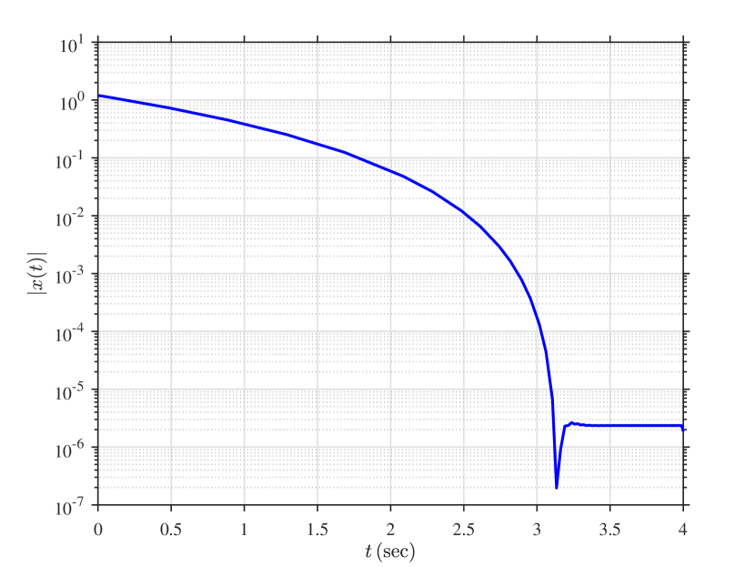
(a) Numerical Simulation of Eqn. (14) with initial condition $x(0)=1.2$. Settling time is estimated as $t_{f}=3.14s$.

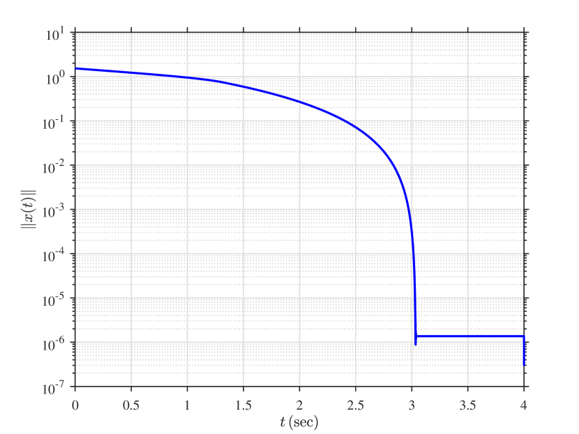
(b) Numerical Simulation of Eqn. (15) with initial condition $x_{1}(0)=1.3$, $x_{2}(0)=.8$. Settling time is estimated as $t_{f}=3.03s$.

Figure 1: Semilog plots of the evolution of the norm of the state for simulation of System (14) (a) and System (15) (b) with specified initial conditions. Settling time is taken as the smallest $t$ for which $\lVert{x(t)}\rVert\leq 10^{-6}$.

Example 10

Consider the 2-state system given by

$$\begin{bmatrix}\dot{x}_{1}(t)\\ \dot{x}_{2}(t)\end{bmatrix}=\underbrace{\begin{bmatrix}-\operatorname{sgn}(x_{1}(t))|x_{1}(t)|^{1/2}+x_{2}(t)^{1/3}\\ -x_{2}(t)^{1/3}\end{bmatrix}}_{f(x(t))}$$ (15)

We now apply Prop. 8 on the domain $\mathcal{D}\subset\mathbb{R}^{2}$, with $\Omega=\{x\in\mathcal{D}:\|x\|^{2}\leq 3\}$ where $q=[q_{1},q_{2}]=[2,3]$, $p=4$, $d=3$, $\tau=2$, $g(x)=3-(x_{1}^{2}+x_{2}^{2})$, and $\lambda_{1}=\lambda_{2}=2$ so that $\prod_{i=1}^{2}|x_{i}|^{\lambda_{i}}=x_{1}^{2}x_{2}^{2}$ . Then

$$\tilde{f}_{1}(\operatorname{sgn}(x)\cdot|x|^{q}) =\half f_{1}(\operatorname{sgn}(x)\cdot|x|^{q})(|x_{1}|^{2})^{-\half}$$

and since $(\operatorname{sgn}(x_{2})|x_{2}|^{3})^{1/3}=x_{2}$, $\operatorname{sgn}(\operatorname{sgn}(x_{1})|x_{1}|^{2})=\operatorname{sgn}(x_{1})$ and $|\operatorname{sgn}(x_{1})|x_{1}|^{2}|^{\half}=|x_{1}|$, we have:

$$\tilde{f}_{1}(\operatorname{sgn}(x)\cdot|x|^{q}) =-\half(x_{1}-x_{2})\frac{1}{|x_{1}|}.$$

Furthermore,

$$\tilde{f}_{2}(\operatorname{sgn}(x)\cdot|x|^{q}) =-\frac{1}{3}x_{2}|\operatorname{sgn}(x_{2})|x_{2}|^{3}|^{-2/3}$$

$$=-\frac{1}{3}x_{2}|x_{2}|^{-2}=-\frac{1}{3}\frac{1}{x_{2}}.$$

Hence,

$$\tilde{f}(\operatorname{sgn}(x_{1})|x_{1}|^{2},\operatorname{sgn}(x_{2})|x_{2}|^{3})=\begin{cases}-\frac{1}{2}(x_{1}-x_{2})\frac{1}{|x_{1}|},\\ -\frac{1}{3}\frac{1}{x_{2}}.\end{cases}$$

Since

$$\nabla_{x}V(x)^{T}\tilde{f}(\operatorname{sgn}(x)|x|^{q})\prod_{i=1}^{n}|x_{i}|^{2\lambda_{i}}$$

$$=-\frac{1}{2}\nabla_{x_{1}}V(x)(x_{1}-x_{2})\frac{1}{|x_{1}|}x_{1}^{2}x_{2}^{2}-\frac{1}{3}\nabla_{x_{2}}V(x)\frac{1}{x_{2}}x_{1}^{2}x_{2}^{2}$$

$$=-\frac{1}{2}\nabla_{x_{1}}V(x)(x_{1}|x_{1}|x_{2}^{2}-|x_{1}|x_{2}^{3})-\frac{1}{3}\nabla_{x_{2}}V(x)x_{1}^{2}x_{2},$$

condition (12) becomes

$$\frac{1}{2}\nabla_{x_{1}}V(x)(x_{1}|x_{1}|x_{2}^{2}-|x_{1}|x_{2}^{3})+\frac{1}{3}\nabla_{x_{2}}V(x)x_{1}^{2}x_{2}\\ -\mu\|x\|^{p}x_{1}^{2}x_{2}^{2}-t(x)(3-x_{1}^{2}-x_{2}^{2})\in\Sigma_{s}.$$

where we choose $t\in\Sigma_{s}$ to be of degree $4$. Due to the presence of absolute values, condition (12) is applied separately on two distinct semialgebraic sets. For $x>0$, the absolute value reduces to $|x|=x$, and the constraint is enforced on a semialgebraic set $g_{1}(x)=x$ and hence

$$\frac{1}{2}\nabla_{x_{1}}V(x)(x_{1}^{2}x_{2}^{2}-x_{1}x_{2}^{3})+\frac{1}{3}\nabla_{x_{2}}V(x)x_{1}^{2}x_{2}\\ -\mu\|x\|^{p}x_{1}^{2}x_{2}^{2}-t_{1}(x)(3-x_{1}^{2}-x_{2}^{2})-v_{1}(x)x,$$

where we choose $t_{1},v_{1}\in\Sigma_{s}$ to be of degree $4$. And, for $x<0$, the absolute value reduces to $|x|=-x$, and the constraint is enforced on a semialgebraic set $g_{2}(x)=-x$, hence

$$\frac{1}{2}\nabla_{x_{1}}V(x)(-x_{1}^{2}x_{2}^{2}+x_{1}x_{2}^{3})+\frac{1}{3}\nabla_{x_{2}}V(x)x_{1}^{2}x_{2}\\ -\mu\|x\|^{p}x_{1}^{2}x_{2}^{2}-t_{2}(x)(3-x_{1}^{2}-x_{2}^{2})+v_{2}(x)x,$$

where we choose $t_{2},v_{2}\in\Sigma_{s}$ to be of degree $4$.

Choosing $k=.2$, we bisect on $\mu$ to find the optimal $\mu^{*}=.16$. The resulting $V$ is given by

$$V(x)=0.0160x_{1}^{6}-5.1188\times 10^{-7}x_{1}^{5}x_{2}+0.3493x_{1}^{4}x_{2}^{2}\\ -0.1610x_{1}^{3}x_{2}^{3}+0.2107x_{1}^{2}x_{2}^{4}-0.0101x_{1}x_{2}^{5}+0.1993x_{2}^{6}.$$

Prop. 8 now implies that for $\tilde{\mu}=\mu/k=.802$, $\gamma=p/2d=2/3$, $\tilde{\Omega}:=\{z_{1},z_{2}\in\mathcal{D}:(\operatorname{sgn}(z_{1})|z_{1}|^{1/2},\operatorname{sgn}(z_{2})|z_{2}|^{1/3})\in\Omega\}=\{(x_{1},x_{2})\,:\,|x_{1}|+|x_{2}|^{2/3}\leq 3\}$,

$$\tilde{V}(z)= \;0.016z_{1}^{3}-5.12\cdot 10^{-7}\,\operatorname{sgn}(z_{1})|z_{1}|^{5/2}z_{2}^{1/3}$$

$$\;+0.35z_{1}^{2}z_{2}^{2/3}-0.161\,\operatorname{sgn}(z_{1})|z_{1}|^{3/2}z_{2}$$

$$\;+0.21z_{1}|z_{2}|^{4/3}-0.01\,\operatorname{sgn}(z_{1})|z_{1}|^{1/2}z_{2}^{5/3}+0.2z_{2}^{2}$$

that the settling time function is bounded by $T(z)\leq 3.7405\tilde{V}^{1/3}$ for any $z$ such that $\{x\,:\,\tilde{V}(x)\leq\tilde{V}(z)\}\subset\tilde{\Omega}$. For example, if we take initial state $z_{1}(0)=1.3$ and $z_{2}(0)=0.8$, then $\tilde{V}(z(0))=.676$ and it can be shown (using an auxiliary SoS program) that $\tilde{V}(x)\leq.674$ implies $\lVert{x}\rVert^{2}\leq 3$. Thus, the settling time function is valid for this initial condition and is bounded by $3.28$.

Using this initial condition, the estimated settling time obtained from numerical simulation using MATLAB’s ode-23 solver is $3.03\,\text{s}$. The results of this simulation can be found in Fig. 1(b).

8 Conclusion

In this paper, we have proposed a method for using SoS programming to test finite-time stability and bound the associated settling time function. For finite-time stable systems, the vector field typically has fractional exponents and Lyapunov conditions for finite-time stability likewise involve fractional terms. To eliminate fractional terms from the stability test and vector field, we have proposed a coordinate transformation which yields alternative Lyapunov stability conditions. We have furthermore shown how these alternative stability conditions can be enforced using SoS programming. Numerical examples are used to illustrate the approach and demonstrate accuracy in the resulting settling time function. These results have the potential to be used in sliding mode control to guarantee finite convergence to the sliding surface in sufficiently short time.

References

- Bacciotti and Rosier (2005) Bacciotti, A. and Rosier, L. (2005). Liapunov functions and stability in control theory. Springer Science & Business Media.
- Basin and Ramírez (2014) Basin, M.V. and Ramírez, P.C.R. (2014). A supertwisting algorithm for systems of dimension more than one. IEEE Transactions on Industrial Electronics, 61(11), 6472–6480.
- Bhat and Bernstein (1995) Bhat, S.P. and Bernstein, D.S. (1995). Lyapunov analysis of finite-time differential equations. In Proceedings of 1995 American Control Conference-ACC’95, volume 3, 1831–1832. IEEE.
- Bhat and Bernstein (1998) Bhat, S.P. and Bernstein, D.S. (1998). Continuous finite-time stabilization of the translational and rotational double integrators. IEEE Transactions on automatic control, 43(5), 678–682.
- Bhat and Bernstein (2000) Bhat, S.P. and Bernstein, D.S. (2000). Finite-time stability of continuous autonomous systems. SIAM Journal on Control and Optimization, 38(3), 751–766. 10.1137/S0363012997321358.
- Cortés (2006) Cortés, J. (2006). Finite-time convergent gradient flows with applications to network consensus. Automatica, 42(11), 1993–2000.
- Galicki (2015) Galicki, M. (2015). Finite-time control of robotic manipulators. Automatica, 51, 49–54.
- Haimo (1986) Haimo, V.T. (1986). Finite time controllers. SIAM Journal on Control and Optimization, 24(4), 760–770.
- Jarvis-Wloszek et al. (2005) Jarvis-Wloszek, Z., Feeley, R., Tan, W., Sun, K., and Packard, A. (2005). Control applications of sum of squares programming. Positive polynomials in control, 3–22.
- Khalil (1991) Khalil, H.K. (1991). Nonlinear Systems. Prentice Hall, Englewood Cliffs, NJ, 1st edition.
- Kong et al. (2020) Kong, L., He, W., Yang, W., Li, Q., and Kaynak, O. (2020). Fuzzy approximation-based finite-time control for a robot with actuator saturation under time-varying constraints of work space. IEEE transactions on cybernetics, 51(10), 4873–4884.
- Levant (1993) Levant, A. (1993). Sliding order and sliding accuracy in sliding mode control. International journal of control, 58(6), 1247–1263.
- Mendoza-Avila et al. (2017) Mendoza-Avila, J., Moreno, J.A., and Fridman, L. (2017). An idea for lyapunov function design for arbitrary order continuous twisting algorithms. In 2017 IEEE 56th Annual Conference on Decision and Control (CDC), 5426–5431. IEEE.
- Moreno and Osorio (2012) Moreno, J.A. and Osorio, M. (2012). Strict lyapunov functions for the super-twisting algorithm. IEEE transactions on automatic control, 57(4), 1035–1040.
- Moulay and Perruquetti (2006) Moulay, E. and Perruquetti, W. (2006). Finite time stability and stabilization of a class of continuous systems. Journal of Mathematical Analysis and Applications, 323(2), 1430–1443.
- Papachristodoulou and Prajna (2005) Papachristodoulou, A. and Prajna, S. (2005). Analysis of non-polynomial systems using the sum of squares decomposition. In Positive polynomials in control, 23–43. Springer.
- Parrilo (2000) Parrilo, P.A. (2000). Structured semidefinite programs and semialgebraic geometry methods in robustness and optimization. California Institute of Technology.
- Polyakov and Fridman (2014) Polyakov, A. and Fridman, L. (2014). Stability notions and lyapunov functions for sliding mode control systems. Journal of the Franklin Institute, 351(4), 1831–1865.
- Polyakov and Poznyak (2012) Polyakov, A. and Poznyak, A. (2012). Unified lyapunov function for a finite-time stability analysis of relay second-order sliding mode control systems. IMA Journal of Mathematical Control and Information, 29(4), 529–550.
- Prajna et al. (2005) Prajna, S., Papachristodoulou, A., Seiler, P., and Parrilo, P.A. (2005). Sostools and its control applications. Positive polynomials in control, 273–292.
- Putinar (1993) Putinar, M. (1993). Positive polynomials on compact semi-algebraic sets. Indiana University Mathematics Journal, 42(3), 969–984.
- Roxin (1966) Roxin, E. (1966). On finite stability in control systems. Rendiconti del Circolo Matematico di Palermo, 15(3), 273–282.
- Savageau and Voit (1987) Savageau, M.A. and Voit, E.O. (1987). Recasting nonlinear differential equations as s-systems: a canonical nonlinear form. Mathematical biosciences, 87(1), 83–115.
- Seeber et al. (2018) Seeber, R., Reichhartinger, M., and Horn, M. (2018). A lyapunov function for an extended super-twisting algorithm. IEEE Transactions on Automatic Control, 63(10), 3426–3433.
- Srinivasan et al. (2018) Srinivasan, M., Coogan, S., and Egerstedt, M. (2018). Control of multi-agent systems with finite time control barrier certificates and temporal logic. In 2018 IEEE Conference on Decision and Control (CDC), 1991–1996. IEEE.
- Topcu et al. (2008) Topcu, U., Packard, A., and Seiler, P. (2008). Local stability analysis using simulations and sum-of-squares programming. Automatica, 44(10), 2669–2675.
- Torres-Gonzalez et al. (2017) Torres-Gonzalez, V., Sanchez, T., Fridman, L.M., and Moreno, J.A. (2017). Design of continuous twisting algorithm. Automatica, 80, 119–126.
- Venkataraman and Gulati (1990) Venkataraman, S.T. and Gulati, S. (1990). Terminal slider control of nonlinear systems. In Proceedings of the International Conference on Advanced Robotics.
- Wang and Xiao (2010) Wang, L. and Xiao, F. (2010). Finite-time consensus problems for networks of dynamic agents. IEEE Transactions on Automatic Control, 55(4), 950–955.
- Zhao et al. (2010) Zhao, D., Li, S., Zhu, Q., and Gao, F. (2010). Robust finite-time control approach for robotic manipulators. IET control theory & applications, 4(1), 1–15.