Local Limits of Small World Networks

Abstract.

Small-world networks, known for their high local clustering and short average path lengths, are a fundamental structure in many real-world systems, including social, biological, and technological networks. We apply the theory of local convergence (Benjamini-Schramm convergence) to derive the limiting behavior of the local structures for two of the most commonly studied small-world network models: the Watts-Strogatz model and the Kleinberg model. Establishing local convergence enables us to show that key network measures—such as PageRank, clustering coefficients, and maximum matching size—converge as network size increases, with their limits determined by the graph’s local structure. Additionally, this framework facilitates the estimation of global phenomena, such as information cascades, using local information from small neighborhoods. As an additional outcome of our results, we observe a critical change in the behavior of the limit exactly when the parameter governing long-range connections in the Kleinberg model crosses the threshold where decentralized search remains efficient, offering a new perspective on why decentralized algorithms fail in certain regimes.

1. Introduction

It is well established that many real-world networks, such as social networks, biological systems, and technological infrastructures, exhibit small-world properties [29, 41, 15]. Over the years, many models have been developed to understand how these small-world networks function, with the Kleinberg [30] and Watts-Strogatz [45] models being two of the most extensively studied. These models have deepened our understanding of many phenomena, ranging from neural connectivity and brain function in biological systems [8] to the study of social sciences [42], and the design of computer chips [33].

A key challenge in the study of small-world networks is understanding how various network properties—such as clustering coefficients, PageRank, network dynamics like the spread of epidemics, and the performance of decentralized algorithms—evolve as networks grow larger. Traditionally, these properties have been analyzed in isolation, each requiring its own proof techniques for demonstrating convergence and concentration. However, imagine if we could define a limit object for our graph models—this would inherently ensure the convergence and concentration of these local properties, thereby simplifying the analysis significantly. With such a framework, local information from just a small neighborhood of nodes could be leveraged to estimate global phenomena, such as the spread of information throughout social networks. This framework is known as local convergence (also known as Benjamini Schramm convergence [10]), and it has been well-developed for various random graph models [12, 44, 34].

In this paper, we establish the local limit of two of the main small-world models—the Kleinberg model [30] and the Watts-Strogatz model [45] (Theorems 3.1, 3.3 and 3.5). The theory of local limits is well-established, providing a powerful framework: for any graph with a local limit, any local property—such as PageRank, clustering coefficients, or the asymptotic size of a maximum matching—immediately converges to the corresponding measure on the limit graph [26, 23, 14]. This means that once we determine the local graph limit, we can immediately derive the limits of a wide variety of local network measures, implying convergence of many network properties. Moreover, in some cases, the local behavior of network dynamics can also yield insights into global properties [35, 2]. For example, as an application of our result on local convergence of small-world networks, the global behavior of information cascades or epidemics can be estimated using only small local samples (see Section 4).

Next, we review the definition of local convergence of graphs, describe the small-world models studied in this paper, and state our main results followed by their applications.

2. Local Convergence

To describe the limiting objects we use the theory of local convergence. The foundational framework of this theory was initiated independently by Aldous and Steele [1] as well as by Benjamini and Schramm [10]. At a high level, a sequence of graphs $(G_{n})_{n\in\mathbb{N}}$ is said to exhibit local convergence if the empirical distribution governing the neighborhoods of randomly chosen nodes converges to a limit distribution. The chosen node can be seen as a root. The limit is then a probability measure $\mu$ on the space of rooted, locally finite graphs (denoted by $\mathcal{G}_{*}$ ). This definition can be extended to the case where each node and edge in $G_{n}$ is accompanied by a mark, which can take values in any complete separable metric space (in this paper, the metric space is a subspace of vector of real numbers). To define convergence rigorously, we must introduce a metric on the space of (marked) rooted graphs.

Definition 2.1.

A rooted graph $(G,o)$ is a graph $G$ with a node labeled as root $o\in V(G)$. A marked rooted graph $(G,o,M(G))$ is a rooted graph $(G,o)$ together with a set $M(G)$. Here, $M(G)$ (the mark) maps $V(G)$ and $E(G)$ to a complete separable metric space $\Xi$.

Definition 2.2 (Metric on marked rooted graphs $\mathscr{G}_{*}$).

Let $(G_{1},o_{1},M(G_{1}))$ and $(G_{2},o_{2},M(G_{2}))$ be two rooted connected graphs, and $B_{r}(G,o)$ denote the (rooted) marked subgraph of $(G,o)$ of all nodes at graph distance at most $r$ away from $o$. Let $d_{\Xi}$ be a metric on the space of marks $\Xi$. The distance metric that allows $\mathscr{G}_{*}$ to be interpreted as a metric space is as follows:

$$d_{\mathscr{G}_{*}}((G_{1},o_{1},M_{1}),(G_{2},o_{2},M_{2}))=\frac{1}{1+R^{*}}$$

where

$$R^{*} =sup\{r:B_{r}(G_{1},o_{1})\simeq B_{r}(G_{2},o_{2}),$$

$$\exists\text{ }\pi\text{ such that }d_{\Xi}(M_{1}(u),M_{2}(\pi(u))\leq 1/r\text{ for all }u\in V(B_{r}(G_{1},o_{1})),$$

$$d_{\Xi}(M_{1}((u,v)),M_{2}(\pi((u,v)))\leq 1/r\text{ for all }(u,v)\in E(B_{r}(G_{1},o_{1}))\},$$

where $\pi:V(B_{r}(G_{1},o_{1}))\to V(B_{r}(G_{2},o_{2}))$ running over all isomorphisms between $B_{r}(G_{1},o_{1})$ and $B_{r}(G_{2},o_{2})$.

With this metric in place, we are now prepared to define local convergence on the space of rooted graphs. We use the following definition, which is equivalent to the original definition given in [10], as demonstrated in [28, Theorem 2.15].

Definition 2.3 (Local Convergence in Probability).

Let $(G_{n},M_{n})_{n\geq 1}$ be a sequence of random graphs. Then $(G_{n},M_{n})_{n\geq 1}$ converges locally in probability to $(G,o,M)\sim\mu$, when for any $\epsilon>$, all integers $r>0$, and any marked rooted graph $H_{*}=(H_{*},o_{*},M_{*})$,

$$\frac{1}{n}\sum_{o_{n}\in V(G_{n})}\mathbbm{1}_{r}^{\epsilon}((G_{n},o_{n})\simeq H_{*})\overset{\mathbb{P}}{\to}\mu(\mathbbm{1}_{r}^{\epsilon}((G,o)\simeq H_{*}))$$

where $\mathbbm{1}_{r}^{\epsilon}$ is defined as the indicator that $r$ neighborhood of $(G_{n},o_{n})$ and $(H_{*},o_{*})$ are isomorphic, and the distance of the corresponding marks are bounded by $\epsilon$. Formally,

$$\mathbbm{1}_{r}^{\epsilon}((G_{n},o_{n})\simeq(H_{*},o_{*},M_{*}))=\mathbbm{1}\Big{(}B_{r}(G_{n},o_{n})\simeq B_{r}(H_{*},o_{*})\text{ and}$$

$$\exists\pi\text{ such that,}\max_{u\in V(B_{r}(H_{*},o_{*}))}d_{\Xi}(M_{n}(u),M_{*}(\pi(u)))<\epsilon$$

$$\max_{uv\in E(B_{r}(H_{*},o_{*}))}d_{\Xi}(M_{n}(u,v),M_{*}(\pi(u,v)))<\epsilon\Big{)}$$

where $\pi$ runs over all isomorphisms between $B_{r}(G_{n},o_{n})$ and $(H_{*},o_{*})$.

This definition implies that a sequence of graphs is said to converge if the empirical frequencies of subgraphs, with an $\epsilon$-tolerance for error in the marks, converge to a limiting distribution. For more on local convergence see [28, Chapter 2].

3. Main Results

We are now ready to state the main results. For each of the small-world networks, we start by defining the models first, and then we describe the local limits.

3.1. Watts-Strogatz Model

The Watts-Strogatz model [45] provided one of the earliest understandings of how small-world properties can emerge from simple modifications to network structure. In their original model, the network starts as a regular ring lattice. Then, a small fraction of these edges are randomly rewired, introducing shortcuts between distant parts of the network. The model can be formally described as follows (see Figure 1 for an illustration with $k=2$):

• Construct the Initial Network: Start with a cycle of $n$ nodes. Connect each node to its $k$ nearest neighbors on either side, forming a regular ring lattice. This structure is called a $k$-ring (where $k$ is a constant independent of $n$).

• Rewire Edges: Direct all edges in a clockwise direction. Rewire each edge’s endpoint (the outgoing end) with probability $\phi$ to a uniformly selected node. Finally, the graph is made undirected by treating all edges as bidirectional.

In this model, the rewired edges are referred to as shortcuts, while the original, non-rewired edges are called ring edges. Also, we refer to both shortcuts and ring edges as incoming or outgoing based on their direction relative to the clockwise orientation in the construction above. We denote the small-world network generated by this procedure with parameters $n$, $\phi$, and $k$ as $WS(n,\phi,k)$. Next, we describe the limit denoted by $WS(\phi,k)$.

Figure 1. $WS(12,\phi,2)$ increasing randomness from left to right: for $\phi=0$, $0<\phi<1$, $\phi=1$ respectively. Colored edges correspond to shortcuts while black edges correspond to ring edges. Arrows indicate the directions of edges in the Watts-Strogatz process but the final graphs are undirected.

3.2. Local Limits of Watts-Strogatz Model

We approach the problem by first examining the limit structure of the initial network (the $k$-ring) and then introducing the rewiring process in the limit. The local limit of the $k$-ring is an infinite graph, constructed as follows: Start with a rooted infinite path and connect each node to its $k$-nearest neighbors. This results in a graph where every node has exactly $2k$ neighbors, a configuration we call the Full $k$-Path. We define the outgoing edges as the connections from a node to its $k$ nearest neighbors on its right-hand side. As an extension of the Full $k$-Path, we define a reduced version of the Full $k$-Path (called Reduced $k$-Path) with the key difference that the root node has only $k-1$ outgoing edges (one of the original $k$ outgoing edges is removed uniformly at random). We now define the $k$-Fuzz structures, incorporating the randomness introduced by rewiring edges in the Watts-Strogatz model.

$k$-Fuzz structures

To construct a Full $k$-Fuzz, start with a Full $k$-path and, for each node in the network, consider its $k$ outgoing ring edges. Keep each edge independently with probability $1-\phi$, and rewire it with probability $\phi$. Upon rewiring, the outgoing shortcut connects to the root of a new Full $k$-Fuzz, thereby initiating a new independent process of Full $k$-Fuzz construction. Additionally, each node has $\text{Poi}(k\times\phi)$ incoming shortcuts, where the other endpoint of each of these incoming edges connects to the root of a Reduced $k$-Fuzz. The Reduced $k$-Fuzz differs only in that the construction starts from a Reduced $k$-Path. The processes for rewiring and connecting shortcuts remain identical. Finally, the graph is made undirected by treating all edges as bidirectional.

Figure 2. Local limit structure of a full $k$-fuzz (for $k=2$). The outgoing shortcut from the root (shown in red) connects to a full $k$-fuzz, while the incoming shortcut connects to a reduced $k$-fuzz.

Let $WS(\phi,k)$ denote the measure in the space of rooted graphs that describe the Full $k$-Fuzz process above. Our first main result formally establishes $WS(\phi,k)$ as the local limit of $WS(n,\phi,k)$.

Theorem 3.1 (Local Limit of the Watts-Strogatz model).

For any integer $k\geq 1$, Watts-Strogatz’s model converges locally in probability to the Full $k$-Fuzz described above, i.e., $WS(n,k,\phi)\overset{\mathbb{P}}{\to}WS(k,\phi)$ as $n\to\infty$.

To understand the intuition behind the local limit of the Watts-Strogatz model, consider the structure rooted at a uniformly chosen node. As we explore the network from this root, different scenarios happen depending on whether we traverse through incoming shortcuts or outgoing shortcuts. When we traverse a shortcut, with a high probability, we reach a node far enough from the root such that its local neighborhood is independent of the original node’s neighborhood. This results in an independent $k$-fuzz process rooted at the target node. However, the degree of the target node within the $k$-fuzz depends on the type of shortcut: 1) If we traverse an incoming shortcut to reach the target node, then one of the $k$ outgoing ring edges of the target node has been rewired to the original root. This leaves $k-1$ remaining edges at the target node that could potentially be rewired, hence the rest of the process described by a Reduced $k$-Fuzz. 2) If we traverse an outgoing shortcut, we encounter a Full $k$-Fuzz, as all $k$ edges are available for potential rewiring.

To formalize the proof of the theorem, we need to rigorously demonstrate that the shortcuts do not appear in local cycles, unlike the ring edges (see Lemma 7.5). In fact, when $k=1$ even the ring edges do not create cycles, leading to a tree-like structure characterized by a multi-type branching process as shown in Corollary 3.2. In the formal proof, we carefully track whether each edge is a shortcut or a ring edge, and how far the endpoints are from each other in the original $k$-ring neighbors which can range from $1$ to $k$ (in total, this requires tracking $4k$ edge marks). We prove convergence with respect to these edge marks, using a second-moment argument in Section 7.

Corollary 3.2.

When $k=1$, Watts-Strogatz’s model converges locally in probability to a multi-type branching process with $4$ types.

3.3. Kleinberg Model

Figure 3. $K(9,2,2,\ell)$ for some $\ell$. For simplicity, we plot the directed edges that only belong to the center node in the lattice and colored edges based on the type.

Another celebrated model is the Kleinberg model [30], which extends the study of small-world networks by focusing on the efficiency of decentralized search. In this model, nodes are placed on a $n\times n$ lattice (so that the total number of nodes is $n^{2}$), with the lattice distance between nodes $u=(u_{x},u_{y})$ and $v=(v_{x},v_{y})$ defined as $d(u,v)=|u_{x}-v_{x}|+|u_{y}-v_{y}|$. Each node is connected to all others within a lattice distance $k$, forming directed lattice connections. The result is called a $k$-lattice.

To incorporate long-range connections, each node $v$ independently selects $q$ directed shortcuts. The probability of connecting to another node $u$ is proportional to $[d(u,v)]^{-\ell}$, where $d(u,v)$ is the lattice distance, and $\ell$ is the power-law exponent that determines how connection probabilities decay with distance. Note that the normalization factor is $\sum_{u}[d(u,v)]^{-\ell}$ to ensure that these probabilities form a valid distribution. We denote the graph sampled through this procedure as $K(n,q,k,\ell)$ (see Figure 3).

A key insight from [30] highlights how the distribution of long-range shortcuts affects the efficiency of decentralized search. Specifically, for $\ell=2$, short paths can be efficiently found using a simple greedy algorithm, whereas for other values of $\ell$, no local algorithm can efficiently discover the shortest path (see Section 4.1). Similarly, we identify $\ell=2$ as a critical point for the Kleinberg model. The local limit of $K(n,q,k,\ell)$ undergoes a phase transition at $\ell=2$, exhibiting distinct behaviors for $\ell\leq 2$ and $\ell>2$.

3.4. Local Limit of the Kleinberg Model ($\ell\leq 2$)

To describe the local limit of the Kleinberg model, we first note that a node’s coordinates within the lattice influence both its in-degree and the coordinates of its neighbors through these incoming and outgoing shortcuts. For example, for a node with mark $u$, the expected number of incoming shortcuts (denoted as $\Lambda_{u}^{(n)}$) is given by (Figure 6):

$$\Lambda_{u}^{(n)}=q\sum_{\begin{subarray}{c}w\neq u\\ w\in V(G_{n})\end{subarray}}\frac{[d(w,u)]^{-\ell}}{\sum_{\begin{subarray}{c}v\neq w\\ v\in V(G_{n})\end{subarray}}[d(w,v)]^{-\ell}}.$$

To incorporate this, we treat the Kleinberg model as a marked graph, where the mark of each node is its lattice coordinate normalized by $n$ in $M=[0,1]\times[0,1]$ accompanied with the $L_{1}$ norm metric.

The second observation is that when $\ell\leq 2$, shortcuts originating from a given node are highly unlikely to connect to nodes within its local neighborhood. Instead, with high probability, each shortcut connects to a node in a distant and independent region of the lattice (see Lemma 8.4). Moreover, when a shortcut is traversed, the mark of its endpoint is sampled from a distribution that depends on the mark of the originating node. To formalize this intuition, we define the limit for $\ell\leq 2$ by defining a $(q,k)$-patch.

A $(q,k)$-patch is a rooted graph constructed by connecting different marked $k$-lattices, where nodes within each lattice share the same marks, and the lattices with different marks are connected as follows.

• The Base Lattice: Begin with a rooted infinite $k$-lattice, referred to as the base lattice. All the nodes in this lattice share the same mark $m$ sampled uniformly from $M=[0,1]\times[0,1]$.

• Outgoing Shortcuts with Marks: In a lattice marked $m$, each node is assigned $q$ outgoing shortcuts. Each shortcut connects to a target node in a new, independent $(q,k)$-patch. The lattice containing the target node is assigned a distinct mark sampled from:

  $$p_{\text{out},m}(m_{\text{out}}):=\frac{\|m-m_{out}\|_{1}^{-\ell}}{\int_{\begin{subarray}{c}x\in[0,1]\times[0,1]\end{subarray}}\|m-x\|_{1}^{-\ell}dx}.$$

  This reflects the distance-dependent distribution of shortcuts in the Kleinberg model.

• Incoming Shortcuts with Marks: Each node with mark $m$ has i.i.d. $\text{Poi}(\Lambda_{m})$ incoming shortcuts, where

  $$\Lambda_{m}=q\int_{w\in[0,1]\times[0,1]}p_{\text{out},w}(m)dw.$$

  These incoming shortcuts connect to new independent reduced $(q,k)$-patches structures, where all the nodes in their base lattice share the same mark, $m_{\text{in}}$, sampled from the following distribution:

  $$p_{\text{in},m}(m_{in}):=\frac{q}{\Lambda_{m}}p_{\text{out},m}(m_{in}).$$

  Here, the reduced $(q,k)$-patch is analogous to the $(q,k)$-patch with the only difference being that the root has $q-1$ outgoing shortcuts.

• Recursive Structure with Marks: The process of assigning marks and creating shortcuts repeats recursively for all nodes in both the outgoing and incoming $(q,k)$-patches.

The next theorem describes the limit of the Kleinberg model.

Theorem 3.3 (Local limit of the Kleinberg model ($\ell\leq 2$)).

For any integers $k$ and $q>0$, $\ell\leq 2$, the Kleinberg model $K(n,q,k,\ell)$ converges locally in probability to $K(q,k,\ell)$ sampled from the $(q,k)$-patch process.

Remark 3.4 (Hidden random tree).

As a result of the construction of the limiting graph, the subgraphs induced by the shortcuts in $K(q,k,\ell)$ converge in probability to a multitype branching process, when $\ell\leq 2$.

The proof of this theorem for the case of $\ell\leq 2$ is based on showing that shortcuts originating from a node connect, with high probability, to distant and independent regions of the lattice. A key element of the argument is a lemma ensuring that shortcuts do not form short cycles, thereby maintaining the tree-like structure of the shortcuts—a crucial property for the limit to converge to a multi-type branching process. In the proof, we also rely on a coupling argument that aligns the continuous marks of the shortcuts in the limiting graph with the discrete marks in the finite case, while carefully tracking changes in the degree distribution to establish the convergence of the first and second moment of subgraph frequencies.

3.5. Local Limit of the Kleinberg Model ($\ell>2$)

For $\ell>2$, the local limit of the Kleinberg model exhibits a fundamentally different behavior compared to the case $\ell\leq 2$. In this regime, shortcuts are local, connecting nodes within a bounded lattice distance. To formalize this, we introduce the normalization constant $\zeta(\ell)=\sum_{d=1}^{\infty}d^{-\ell}$, which is finite and well-defined for $\ell>2$ due to the convergence of the Riemann zeta function. The probability of a shortcut connecting a node $u$ to another node $v$ at lattice distance $d(u,v)$ is given by $\kappa(u,v)=\frac{d(u,v)^{-\ell}}{\zeta(\ell)}$. Here $\kappa:\mathbb{Z}\times\mathbb{Z}\to[0,1]$ is the kernel defining the probability distribution of connections.

The limiting graph $K(q,k,\ell)$ is constructed as follows: Starting with an infinite $k$-lattice, each node is assigned $q$ outgoing shortcuts, where the endpoint of each shortcut is chosen independently according to the kernel $\kappa$. The following theorem establishes the convergence of the finite Kleinberg model to this limiting structure.

Theorem 3.5 (Local limit of the Kleinberg model ($\ell>2$)).

For any integers $k>0$, $q>0$, and $\ell>2$, the Kleinberg model $K(n,q,k,\ell)$ converges locally in probability to the graph $K(q,k,\ell)$.

The first step of the proof is to establish that shortcuts in both the finite graph and the limit graph are confined within a bounded lattice distance. This step is essential for ensuring that the construction of the limiting graph is well-defined and remains local. For this purpose we establish a connection between local graph neighborhoods and lattice neighborhoods. Specifically, for any graph distance $r$, we prove the existence of a lattice distance $R$ such that the graph neighborhood of radius $r$ is contained within the lattice neighborhood of radius $R$. This is achieved using a path-counting argument to show that any path of length $R$, potentially containing shortcuts, is confined within a bounded lattice distance (Lemma 9.6). This step adapts techniques from the beautiful work of [44], with the specific adaptations being detailed later. Next, we prove the convergence of lattice neighborhoods. This step is simplified compared to handling shortcuts, as we do not need to track shortcut connections to infinity. The convergence is established using a second-moment argument, ensuring that the neighborhoods of two uniformly chosen nodes are asymptotically independent (Lemmas 9.4 and 9.5).

As stated earlier the path-counting argument is similar to the techniques developed for spatial inhomogeneous random graphs (SIRGs) [44]. However, some modifications are required to handle the unique features of the Kleinberg model. In the SIRG framework, nodes are embedded in a spatial structure, and edges between any two nodes arise independently with probabilities governed by a kernel function that depends on their spatial distance. By contrast, in the Kleinberg model, the number of shortcuts is a deterministic constant $q$ per node, which changes the way randomness operates in long-range connections.

4. Applications

By proving local convergence for small-world networks, we gain powerful tools to analyze a wide range of network properties, both about network structures and different dynamics over networks. Below, we outline several key applications of Theorems 3.1, 3.3, and 3.5.

4.1. Phase Transition and Kleinberg’s Local Algorithm

Kleinberg considered a simple greedy algorithm to find a path from the source to the target. This algorithm starts from the source node and, at each step, it moves to the neighbor that is closest to the target destination until the target is reached [30]. In particular, Kleinberg showed that this local algorithm is most efficient when $\ell=2$: while we reach the target in $O(\log n)^{2}$ when $\ell=2$, the expected time is significantly larger ($n^{\alpha}$ for some $\alpha>0$) for other values of $\ell$.

Our result in Theorems 3.3 and 3.5 provide an alternative explanation for this phenomenon. As the power-law exponent $\ell$ crosses the threshold of $2$, the network’s local structure undergoes significant changes. When $\ell>2$, the local limit reveals that all node marks are equal within a neighborhood, indicating that shortcuts only connect nodes within very short distances. This structural change explains why Kleinberg’s decentralized search algorithm becomes inefficient in this regime: the shortcuts fail to support long-range navigation.

Conversely, when $\ell\leq 2$, the graph induced by shortcuts converges to a tree-like structure, ensuring strong global connectivity. However, the regime of $\ell<2$ has another challenge: the distance between the two ends of a shortcut is bounded below by $\Omega(n)$ (Lemma 8.4). Thus, once the decentralized search algorithm gets suitably close to the target person, all shortcuts will connect further away from the target, making the shortcuts ineffective.

The case of $\ell=2$ is unique. Here, shortcuts can connect nodes with both different and identical marks. As established in Lemma 8.4, the distance $d$ between the two ends of a shortcut satisfies $\log(d)=\Omega(\log(n))$, allowing for sublinear distances as well. Note that the marks of two nodes with $o(n)$ distance converges to the same value in the limit. Consequently, at $\ell=2$, the shortcuts are effective not only when the target is far but also when it is near, leading to an optimal scenario for a decentralized search algorithm.

4.2. Clustering Coefficient

The clustering coefficient is a measure of interconnectedness in small-world networks, where high clustering is a key feature. The local clustering coefficient $C(v)$ of a node $v$ quantifies the likelihood that two neighbors of $v$ are also neighbors, while the global clustering coefficient $C_{\text{global}}$ provides an aggregate measure of clustering across the entire graph:

$$C(v)=\frac{\Delta_{G}(v)}{d_{v}(d_{v}-1)}\quad\quad C_{\text{global}}=\frac{\sum_{v\in V}\Delta_{G}(v)}{\sum_{v\in V}d_{v}(d_{v}-1)}.$$

Here, $d_{v}$ denotes the degree of node $v$ and $\Delta_{G}(v)=\sum_{u,w\in\partial B_{1}(v)}\mathbbm{1}_{\{\{u,w\}\in E(G)\}}$ denotes twice the number of triangles in $G$ that contain $v$.

Proving local convergence for small-world networks allows for the precise calculation of the limiting distributions of both local and global clustering coefficients. It is known that $C(v)$ and $C_{\text{global}}$ are local properties of graphs that have a local limit (Theorem 2.22 and 2.23 in [28]). So, by applying the main theorems of this paper, one can prove the locality of the clustering coefficient for small-world networks. Moreover, because of the fact that shortcuts create locally tree-like structures (as shown in Lemmas  7.5 and 8.4), the limiting distribution of clustering coefficients only depends on the non-shortcut edges, leading to the following corollaries.

Corollary 4.1 (Clustering Coefficient of Watts-Strogatz Model).

Let $C(v)$ be local and $C_{\text{global}}$ be global clustering coefficients of $WS(n,\phi,k)$. Then,

$$C_{\text{global}}\xrightarrow{\mathbb{P}}\frac{3(k-1)}{2(2k-1)+\phi(2-\phi)}(1-\phi)^{3}$$

as $n\to\infty$. Similarly,

$$C(v)\xrightarrow{\mathbb{P}}\mathbb{E}_{\mu}\left[\frac{\Delta_{G}(o)}{d_{o}(do-1)}\right]$$

where $d_{o}$ is the degree of the root $o$, $\Delta_{G}(o)$ is twice the number of triangles that contain $o$ and $\mu$ is distributions specified in Theorem 3.1.

For the analog in the Kleinberg model, let $\Delta_{L_{k}}$ denote twice the number of triangles that include the root in the infinite $k$-lattice. Since infinite the $k$-lattice is deterministic, $\Delta_{L_{k}}$ is also deterministic. Then the following result formalizes the behavior of clustering coefficient in the limit.

Corollary 4.2 (Clustering Coefficient of Kleinberg Model).

Let $C$ be both the local and global clustering coefficients of $K(n,q,k,\ell)$ when $\ell\leq 2$. Then,

$$\text{C}\xrightarrow{\mathbb{P}}\frac{\Delta_{L_{k}}}{(2k(k+1)+q+\Lambda_{m})^{2}-(2k(k+1)+q)}$$

as $n\to\infty$, where $m$ is sampled uniformly from $M$ and $\Lambda_{m}$ is defined as in Theorem 3.3.

These results provide a rigorous foundation for the phase transition in the clustering coefficient of small-world networks that were previously understood through mean-field analyses [38, 7], showcasing the strength of local convergence. Their proofs appear in Appendix C.

4.3. PageRank

PageRank is an algorithm used to rank the importance or centrality of nodes in a graph originally designed to rank World-Wide Web pages. Its applications extend to community detection, citation analysis, and beyond [40]. Garavaglia et al. [26] proved that if a sequence of graphs $G_{n}$ with $n$ nodes converges in probability, then the PageRank of a uniform random node converges in distribution. As an application of this and our main theorems, we get the following corollary.

Corollary 4.3.

The graph normalized PageRank of $WS(n,k,\phi)$ and $K(n,k,q,\ell)$ converges in distribution to a limit.

Importantly, as an artifact of this result, PageRank can be calculated using the local $k$-neighborhood of the root in the graph limit, and the error would decay exponentially in $k$.

4.4. Other Local Functionals

Beyond the applications discussed, local convergence extends to the analysis of various other graph properties. In general, any local graph property—meaning any property that converges for graphs with a local limit—will also converge for the small-world network models studied in this paper. Moreover, these properties can be approximated using small local samples. Two notable examples include the assortivity coefficient [28, Theorem 2.26] and the fraction of nodes appearing in a maximum matching [14].

4.5. Dynamic Processes on Small-World Networks

Local convergence is a powerful tool for understanding dynamic processes on networks, such as the spread of information or diseases. One key application is understanding the spread of epidemics on networks. In the context of the SIR (Susceptible-Infected-Recovered) model, local convergence ensures that the time evolution of the epidemic—such as the fractions of nodes in each state—converges as the network size increases [4]. Moreover, it enables the use of local network samples of a constant number of nodes to predict the spread dynamics. While previous work established these results for general convergent graphs, with our result these insights can be applied to small-world networks as well.

A specific case of epidemic modeling is information cascade, where a single node transmits information through each edge independently with probability $p$. A central question here is determining how many nodes eventually receive the information, which is closely related to the size of the largest component after percolation. Previous work has shown that for expanders with local convergence, the size of the largest component (corresponding to the final number of informed nodes) concentrates around its limit [2]. Given our results and the fact that small-world networks—such as the Kleinberg model (with $\ell\leq 2$)—are known to be expanders [21], we can apply the results of [2] to conclude that the size of the largest component after percolation in small-world networks also concentrates around its limit. This also implies that estimating the largest component of small-world networks is possible using small local samples. A similar argument shows that a general class of network dynamic processes are local on small-world networks [24, 35].

Finally, when considering random digraphs formed by making edges bidirectional and retaining each with probability $p$, local convergence implies the emergence of bow-tie structures [3]–characteristic of real-world networks like the web [16]. This structural insight provides a rigorous foundation for understanding the patterns observed empirically in large directed networks (also seen in social and financial networks [36, 6]).

5. Other Related Work

Small-world networks have been extensively studied due to their unique properties. [22, 39] extended Kleinberg’s model to arbitrary base graphs, showing that the structure of the base graph, combined with long-range connections, influences the performance of greedy algorithms in decentralized search. Other studies confirm how random shortcuts or clustering reshape network distances and connectivity [17, 9, 13]. Another line of work has been given to study of random walks, search algorithms, and routing in small-world networks [20, 22, 39, 27, 19, 37]. Our results complement prior work by establishing the local convergence of small-world networks, allowing for a unified analysis of both local structures and dynamic properties in this class of networks. By proving the local limits of small-world models, we open new avenues for rigorous analysis of network properties and dynamics using local convergence techniques.

Local Convergence of Random Graph Models

Notably, there is a large body of work proving that random graph models converge locally in probability. The class of random network models with local limit in probability includes configuration models, [18],[28, Chapter 4], sparse inhomogeneous random graphs (including stochastic block models) [12], [28, Chapter 3]), preferential attachment models [11, 25], [28, Chapter 5]), random intersection graphs [34, 43], and spatial inhomogeneous random graphs [44]. The latter includes hyperbolic random graphs [32, 31]. Another related work is [13], where they introduce a class of sparse random graphs with high local clustering that converge locally in probability. However, as noted in their paper, this model does not apply to small-world networks, as the mathematical intractability arises from the dependence between edges.

Despite the extensive work on local convergence in random graph models, there has been little focus on proving local convergence for small-world networks. To the best of our knowledge, we are the first to establish the local convergence of small-world networks. The closest related work is by [5], who studied the distance of typical paths in the Watts-Strogatz model and described a branching process governing the structure shortcuts. While they did not prove local convergence in probability, their work inspired our development of the $k$-fuzz structure, which fully characterizes the limit graph of the Watts-Strogatz model and enables us to rigorously prove local convergence in probability. For the Kleinberg model, we are not aware of any prior work that addresses local convergence or provides a comprehensive analysis of its local structure.

Finally, we note that the study of local graph properties and the convergence of local functionals—such as those discussed in this paper, including spectral distributions, the size of independent sets, and other network dynamics [26, 23, 35, 24]—remains an active area of research. Any future results demonstrating that a property is local for convergent graph sequences can be directly applied to small-world network models using the results established in this work.

6. Preliminaries

We begin by introducing some standard asymptotic notation that will be used throughout the paper. For a function $f(n)$ depending on $n$, we write:

• $f(n)=o(g(n))$ if $\lim_{n\to\infty}\frac{f(n)}{g(n)}=0$. This means that $f(n)$ grows strictly slower than $g(n)$, or equivalently, for any $\epsilon>0$, there exists $N>0$ such that $f(n)<\epsilon g(n)$ for all $n>N$.

• $f(n)=\omega(g(n))$ if $\lim_{n\to\infty}\frac{f(n)}{g(n)}=\infty$. In other words, $\frac{f(n)}{g(n)}$ grows unboundedly as $n\to\infty$, regardless of its exact rate of growth.

• $f(n)=O(g(n))$ if there exist positive constants $c$ and $N$ such that $f(n)\leq cg(n)$ for all $n>N$. This means that $f(n)$ grows at most as fast as $g(n)$, up to constant factors, for large $n$.

• $f(n)=\Omega(g(n))$ if there exist positive constants $c$ and $N$ such that $f(n)\geq cg(n)$ for all $n>N$. This means that $f(n)$ grows at least as fast as $g(n)$, up to constant factors, for large $n$.

These notations will allow us to describe the growth behavior of functions and their interplay with graph parameters.

To analyze local limit of a graph sequence, we need to ensure that the graph is locally finite. A graph $G$ is said to be locally finite if the degree of every vertex is finite almost surely, i.e., the degree $d$ of any of node satisfies $\mathbbm{P}[d<\infty]=1$. Notice that this implies that $\mathbbm{P}[|B_{r}(G,v)|<\infty]=1$ for any fixed $r$ and node $v$ in $G$. Before we state the formal proofs, we need to show that $WS(n,\phi,k)$, $WS(\phi,k)$, $K(n,q,k,\ell)$, and $K(q,k,\ell)$ are locally finite to be able to apply the theory of local convergence. This is the content of this section. First, we will consider the Watts-Strogatz model.

Lemma 6.1.

For any integers, $n\geq k$, and any $\phi\in[0,1]$, $WS(n,\phi,k)$ and $WS(\phi,k)$ are locally finite.

Proof.

Notice that the expected degree of a node in both models is bounded by $3k$. By Markov’s inequality, we have $\mathbbm{P}[\text{degree}<\infty]=1$. ∎

Next, we will consider the Kleinberg model.

Lemma 6.2.

Let $K(n,q,k,\ell)$ be defined as in Section 3.3. Then $K(n,q,k,\ell)$ is locally finite.

Proof.

Let $G_{n}$ be $K(n,q,k,\ell)$. The number of lattice connections of any node $u$ of $G_{n}$ is $2k(k+1)$. We know that its outgoing shortcut degree is $q$. Now, we will show that the expected incoming shortcut degree is bounded by $4q$ independent of $n$. Notice that the sum $\sum_{v\neq u}[d(w,v)]^{-\ell}$ will have $n^{2}-1$ terms for all $u\in V(G_{n})$. This sum is maximized when $u$ is the center node and minimized when $u$ is a corner node. Therefore, we have the following two inequalities:

(1) $$\sum_{v\neq u}[d(w,v)]^{-\ell}\geq\sum_{j=1}^{n-1}(j+1)j^{-\ell}+\sum_{j=1}^{n-1}(n-j)(n-1+j)^{-\ell}>\sum_{j=1}^{n-1}j^{1-\ell},$$

In fact, the first inequality above is tight when $u$ is the corner node. Further, for the upper bound (when $u$ is a center node) we get,

(2) $$\sum_{v\neq u}[d(w,v)]^{-\ell}<4\sum_{j=1}^{n-1}j^{1-\ell}.$$

Then, the expected number of incoming shortcuts of node $u$ is given by

$$\Lambda_{u}^{(n)}=q\sum_{w\neq u}\frac{[d(w,u)]^{-\ell}}{\sum_{v\neq w}[d(w,v)]^{-\ell}}\leq\frac{4q\sum_{j=1}^{n-1}j^{1-\ell}}{\sum_{j=1}^{n-1}j^{1-\ell}}\leq 4q.$$

By Markov’s inequality, $K(n,q,k,\ell)$ is locally finite. ∎

Next, we will establish that the limit of the Kleinberg model is locally finite. To prove this, we need to ensure that the number of incoming edges originating from infinitely many nodes is controlled. The following lemma provides the necessary bound to achieve this.

Lemma 6.3.

Let $K(q,k,\ell)$ be the local limit of $K(n,q,k,\ell)$ given by Theorems 3.3 and 3.5. Then $K(q,k,\ell)$ is locally finite.

Proof.

Let the incoming degree of node $u$ in $K(q,k,\ell)$ be $D_{u}$. Since the number of outgoing shortcuts and lattice connections is $2k(k+1)+q$, it suffices to show that $\mathbbm{P}[D_{u}<\infty]=1$. If $\ell\leq 2$, then $\mathbbm{E}[D_{u}]=\Lambda_{m}$ defined in Section 3.4 where $m$ is the mark of node $u$. Since $\Lambda_{m}$ is finite, by Markov’s inequality, $\mathbbm{P}[D_{u}<\infty]=1$.

Now, let’s consider $\ell>2$. In this case, by symmetry, $D_{u}$ will be the same for all $u$. The probability that a shortcut is going to connect to it from node $v$ such that $d(u,v)=d$ is $d^{-\ell}/(4\zeta(\ell-1))$. Then, the moment-generating function of $D_{u}$ is

$$\mathbbm{E}[e^{tD_{u}}] =\prod_{d=1}^{\infty}\left(1-\frac{d^{-\ell}}{4\zeta(\ell-1)}+\frac{d^{-\ell}e^{t}}{4\zeta(\ell-1)}\right)^{4qd}$$

$$=\prod_{d=1}^{\infty}e^{4qd\log\big{(}1+(e^{t}-1)\frac{d^{-\ell}}{4\zeta(\ell-1)}\big{)}}$$

$$\leq\prod_{d=1}^{\infty}e^{4qd\log\big{(}\exp\left((e^{t}-1)\frac{d^{-\ell}}{4\zeta(\ell-1)}\right)\big{)}}$$

$$=\prod_{d=1}^{\infty}e^{q(e^{t}-1)\frac{d^{1-\ell}}{\zeta(\ell-1)}}=e^{q(e^{t}-1)\sum_{d=1}^{\infty}\frac{d^{1-\ell}}{\zeta(\ell-1)}}$$

$$=e^{q(e^{t}-1)}.$$

By applying Chernoff bound, we have

$$\mathbbm{P}[D_{u}<N]=\mathbbm{P}[e^{tD_{u}}<e^{tN}]\geq 1-\mathbb{E}[e^{-tD_{u}}]e^{-tN}\geq 1-e^{q(e^{t}-1)-tN}\to 1$$

as $N\to\infty$. This proves $\mathbbm{P}[D_{u}<\infty]=1$. ∎

Finally, we will state a useful Lemma that we will frequently refer to in our proofs.

Lemma 6.4.

Given integers $r,d\geq 1$ and a random graph $G$ such that $\mathbbm{E}[deg(u)]\leq d$ for all nodes $u$ in $V(G)$, then $\mathbbm{E}[|B_{r}(G,o)|]\leq d^{r}$. Further, for any any (slowly) growing function $f(n)$ with $\lim_{n\to\infty}f(n)=\infty$, and any given $\epsilon>0,$

$$\lim_{n\to\infty}\mathbbm{P}\left[\frac{|B_{r}(G,o)|}{f(n)}\geq\epsilon\right]=0.$$

Proof.

We will prove this by induction on $r$. For $r=1$, $\mathbbm{E}[|B_{1}(G,o)|]=\mathbbm{E}[deg(u)]\leq d$. Now, assume inductively that $\mathbbm{E}[|B_{r}(G,o)|]\leq d^{r}$. Notice that

$$\mathbbm{E}[|B_{r+1}(G,o)|] =\mathbbm{E}[\mathbbm{E}[|B_{r+1}(G,o)||B_{r}(G,o)]]$$

$$\leq\mathbbm{E}[d|B_{r}(G,o)|]=d\mathbbm{E}[deg(u)]=d^{r+1}.$$

The second part of the lemma is an immediate application of Markov’s inequality,

$$\mathbbm{P}\left[\frac{|B_{r}(G,o)|}{f(n)}\geq\epsilon\right]\leq\frac{d^{r}}{\epsilon f(n)}.$$

Note that the right-hand side goes to $0$ since $f$ is a growing function. ∎

As a result of Lemma 6.1 and Lemma 6.2, for $G_{n}=WS(n,\phi,k)$ or $G_{n}=K(n,q,k,\ell)$, $\mathbbm{E}[|B_{r}(G_{n},o_{n})|]$ is bounded (for any $o_{n}\in V(G_{n})$). From now on, we will reference Lemma 6.4 whenever we need to argue that $|B_{r}(G_{n},o_{n})=o(f(n))$ almost surely for any increasing function $f(n)$.

7. Proof of Theorem 3.1

Let $G_{n}$ be the random graph sampled according to $WS(n,\phi,k)$, $o_{n}$ be the root selected uniformly at random from $G_{n}$, and $(G,o)$ be the random graph sampled according to $WS(\phi,k)$ with measure $\mu$ defined as in Theorem 3.1. Define $\mu_{n}$ to be the measure of $(G_{n},o_{n})=(WS(n,k,\phi),o_{n})$. We prove a stronger version of Theorem 3.1, where edges have marks defined as follows.

7.1. Edge Marks and Ordering

Recall the construction of the Watts-Strogatz model from Section 1. At a high level, the edges of $(G_{n},o_{n})$ and $(G,o)$ are divided into two categories: Edges that remain in their original positions in the $k$-ring are called ring edges, while those rewired during the construction are referred to as shortcuts. Each edge is assigned two marks based on the following:

• Ring Distance: This is the minimum number of steps along the original 1-ring subgraph (the cycle) needed to traverse between the two endpoints of an edge. There are $k$ possible values for this mark. Note that this mark remains unchanged after rewiring: for shortcut edges, the ring distance corresponds to the original edge they replaced during the rewiring process.

• Direction of the Edge: During the Watts-Strogatz construction, edges are initially directed before being made bidirectional in the final step. Consider a Breadth-First-Search (BFS) process starting from an arbitrary node. An edge is marked as outgoing if it is explored from the node it stems from. An edge is marked as incoming if it is explored from the node it connects to.

As a result of this process, we have $2k$ different marks for ring edges and $2k$ different marks for shortcuts. Hence, we have $4k$ different marks for edges in total. We use the metric $d_{\Xi}(m_{1},m_{2})=\mathbbm{1}(m_{1}=m_{2})$ for any edge marks $m_{1}$ and $m_{2}$, which would create a compact metric space as required by Definition 2.2.

Now, we will order the edges of $(G_{n},o_{n}),(G,o)$ (and the subgraph $B_{r}(G,o)$, denoted by $H_{*}$) according to the BFS process that starts from the respective root and prioritizes the edges in the following order: outgoing shortcuts, outgoing ring edges, incoming ring edges, and incoming shortcuts, and mark them based on the mark classification above simultaneously. The BFS will break ties between shortcuts arbitrarily while prioritizing ring edges that connect closer nodes to each other. Let $\overline{G_{n}}$, $\overline{G}$, and $\overline{H}_{*}$ be the version of $G_{n},G$ and $H_{*}$ with ordered and marked edges respectively. See Figure 4 for an example with $n=12$ and $k=1$.

Figure 4. (left) Ordered and marked $WS(12,\phi,1)$ (right) viewing same graph as a tree. Since $WS(12,\phi,1)$ can be seen as a tree, there is a $1$-to-$1$ correspondence between the edges and the non-root nodes. Thus, we instead ordered and marked the child of the edge in the BFS with the corresponding edge mark. The root has a special mark.
Marks: root, outgoing ring edge, incoming ring edge, incoming shortcut, outgoing shortcut.

7.2. Main Lemmas

The main idea of the proof is a second-moment argument showing the convergence of the marked Watts-Strogatz model to its limit. To do so, we need the following notation. Given a marked graph $(H_{*},o_{*},M_{*})$, define

(3) $$\mu_{r,n}^{\epsilon}((G_{n},o_{n})\simeq H_{*}):=\mathbbm{E}_{\mu_{n}}[\mathbbm{1}_{r}^{\epsilon}((G_{n},o_{n})\simeq H_{*})],$$

and

(4) $$\mu_{r}^{\epsilon}((G,o)\simeq(H_{*},o_{*})):=\mathbbm{E}_{\mu}[\mathbbm{1}_{r}^{\epsilon}((G,o)\simeq(H_{*},o_{*}))].$$

For the Watts-Strogatz Model, we can let $\epsilon=0$ because of our metric. For simplicity, we will omit the use of $\epsilon$ in this section from now on.

Using the criterion given by Definition 2.3, it suffices to prove the convergence for $(H_{*},o_{*},M_{*})$ where $\mu_{r}(H_{*},o_{*},M_{*})>0$, i.e., the rooted marked graph $B_{r}(H_{*},o_{*},M_{*})$ appears with a positive probability. Sample and fix any graph $H_{*}=B_{r}(H_{*},o_{*},M_{*})\sim\mu$. Given that $r$ is finite, by Lemma 6.1 and Lemma 6.4, any $H_{*}$ considered from now on will be a finite graph. Let $B_{r}(\overline{G},o)=\overline{H}_{*}$ indicate the order equivalence. Notice that this ordering is not unique. However, in the event that $B_{r}(\overline{G},o)=\overline{H}_{*}$, any other ordering of $G$ would give an isomorphic to $H_{*}$ since the underlying structure is not changed. Thus, we get the following identity:

$$\mu_{r}((G,o)\simeq\ H_{*})=\#(H_{*})\cdot\mu_{r}((\overline{G},o)=\overline{H}_{*})$$

where $\#(H_{*})$ is the number of different ways we could order this marked graph based on the BFS rules outlined. Similarly, we have $\mu_{r,n}((G_{n},o_{n})\simeq\ H_{*})=\#(H_{*})\cdot\mu_{r,n}((\overline{G_{n}},o_{n})=\overline{H}_{*})$. Then, it suffices to prove Lemma 7.1 below to show the convergence in probability.

Lemma 7.1 (Local Convergence of Watts-Strogatz Model).

Fix any $r>0$ and $H_{*}=B_{r}(H_{*},o_{*},M_{*})$ such that $\mu_{r}(H_{*},o_{*},M_{*})>0$ where $\mu$ is the measure of $WS(k,\phi)$ defined in section 3.2. Order and mark $G_{n},G$, and $H_{*}$ according to the process outlined in section 7.1 to get $\overline{G_{n}},\overline{G}$ and $\overline{H}_{*}$. Then,

(5) $$\frac{1}{n}\sum_{o_{n}\in V(G_{n})}\mathbbm{1}_{r}((\overline{G_{n}},o_{n})=\overline{H}_{*})\overset{\mathbb{P}}{\to}\mu_{r}((\overline{G},o)=\overline{H}_{*})\quad\text{ as $n\to\infty$.}$$

At a high level, we will use the Second Moment Method to formally prove the convergence. In particular, we will first show that the expectation of the left-hand side in (5) converges to $\mu_{r}((\overline{G},o)=\overline{H}_{*})$ and then show that its variance goes to $0$ with $n$ formalized in the next two Lemmas.

Lemma 7.2 (First Moment: Watts-Strogatz Model).

Fix any $r>0$ and $H_{*}$, and define $\overline{H_{*}},(\overline{G_{n}},o_{n})$, $(\overline{G},o),\mu_{n}$ and $\mu$ as in Lemma 7.1. Then,

$$\mu_{r,n}((\overline{G_{n}},o_{n})=\overline{H}_{*})\to\mu_{r}((\overline{G},o)=\overline{H}_{*})\quad\text{ as $n\to\infty$.}$$

Lemma 7.3 (Second Moment: Watts-Strogatz Model).

Fix any $r>0$ and $H_{*}$ as in Lemma 7.1. Then,

$$\text{Var}\left(\frac{1}{n}\sum_{o_{n}\in V(G_{n})}\mathbbm{1}_{r}((G_{n},o_{n})\simeq H_{*})\right)\to 0\quad\text{ as $n\to\infty$.}$$

Now, assuming these two lemmas, one can easily prove Lemma 7.1.

Proof of Lemma 7.1 and Theorem 3.1

Take any $\epsilon>0$. Then,

$$\lim_{n\to\infty}\mathbb{P}\left[\left|\frac{1}{n}\sum_{o_{n}\in V(G_{n})}\mathbbm{1}_{r}((G_{n},o_{n})\simeq H_{*})-\mu_{n,r}((G_{n},o_{n})\simeq H_{*})\right|\geq\epsilon\right]$$

$$=\lim_{n\to\infty}\mathbb{P}\left[\left|\frac{1}{n}\sum_{o_{n}\in V(G_{n})}\mathbbm{1}_{r}((G_{n},o_{n})\simeq H_{*})-\mu_{r}((G,o)\simeq H_{*})\right|\geq\epsilon\right]\quad\text{by Lemma \ref{ws-1moment}}$$

$$\leq\lim_{n\to\infty}\frac{\text{Var}\left(\frac{1}{n}\sum_{o_{n}\in V(G_{n})}\mathbbm{1}_{r}((G_{n},o_{n})\simeq H_{*})\right)^{2}}{\epsilon^{2}}\quad\text{by Chebyshev's Inequality}$$

$$=0\quad\text{by Lemma \ref{ws-2moment}}$$

which concludes the proof. ∎

The rest of this section is dedicated to the proof of Lemmas 7.2 and 7.3.

Proof of Lemma 7.2

By symmetry, we need to show the following for a given node $o_{n}\in V(G_{n})$:

(6) $$\mu_{n}(B_{r}(\overline{G_{n}},o_{n})=\overline{H}_{*})\to\mu(B_{r}(\overline{G},o)=\overline{H}_{*})\quad\text{ as $n\to\infty$}.$$

Notice that the distribution of ring edges in both $G_{n}$ and $G$ are the same. In fact, the only differences between the respective measures of $G_{n}$ and $G$ are:

• The number of incoming shortcuts of a node in $G$ follows i.i.d. $\text{Poi}(\phi k)$, while the number of incoming shortcuts of each node $u$ in $G_{n}$ follows a binomial distribution, $\text{Bin}\left(nk-c_{u},\frac{\phi}{n}\right)$, where is $c_{u}$ is a correction factor that depends on the number of edges that are rewired to nodes other than $u$.

• Shortcuts can form cycles in $G_{n}$, whereas they induce a tree-like structure in $G$. More precisely, no cycle in $G$ contains a shortcut as an edge.

Next, we bound the probability that each of these two events occurs. Define $T_{i}$ to be the event that $G_{n}$ and $G$ look identical to $H_{*}$ up until the $i$-th step of the BFS process, i.e. the first $i$ nodes explored in both graphs have the same immediate neighborhoods with the same marks, etc. Let $v_{i,n}$ be the $i$-th node in $\overline{G_{n}}$, $v_{i}$ be the $i$-th node in $\overline{G}$, and $x_{i}$ be the number of incoming shortcuts for the $i$-th node in $\overline{H_{*}}$. Then, to prove the convergence in (6), it suffices to prove that, as $n$ grows,

(7) $$\prod_{i\in[\overline{H_{*}}]}\mu_{n}(v_{i,n}\text{ has }x_{i}\text{ incoming shortcuts and no shortcut appears in cycle in }B_{r}(G_{n},o_{n})|T_{i-1})$$

$$\quad\to\prod_{i\in[\overline{H_{*}}]}\mu(v_{i}\text{ has }x_{i}\text{ incoming shortcuts }|T_{i-1})=\prod_{i\in[t]}\frac{e^{-\phi k}(\phi k)^{x_{i}}}{x_{i}!}.$$

The remainder of the proof is dedicated to this convergence.

Define the rewired state of an edge as its final position after the Watts-Strogatz model construction, and the non-rewired state as its original position as part of the ring. Let $G_{n}^{(i,j)}$ denote the graph configuration where an edge is in its rewired state if it has already been explored by the BFS upon reaching the $j$-th shortcut of $v_{i,n}$; otherwise, it remains in its non-rewired state. Note that, if $j$-th shortcut of $v_{i,n}$ does not connect $B_{r}(G_{n}^{(i,j)},o_{n})$ for all $j\leq x_{i}$ and all $i\leq|B_{r}(G_{n},o_{n})|$ (i.e. as the exploration progresses until $B_{r}(G_{n},o_{n})$ is fully discovered), this implies $B_{r}(G_{n},o_{n})$ is guaranteed not to contain any cycles that include a shortcut. Given this, we can divide (7) into the product of the following two parts:

• $\mu_{n}(v_{i,n}\text{ has }x_{i}\text{ incoming shortcuts }|T_{i-1})$

• $\mu_{n}(\cap_{1\leq j\leq x_{i}}\text{$j$-th shortcut of $v_{i,n}$ does not connect $B_{r}(G_{n}^{(i,j)},o_{n})$}|v_{i,n}\text{ has }x_{i}\text{ incoming shortcuts and }T_{i-1})$

and analyze each of them separately. We will later prove the second probability converges to one, which equivalently shows that shortcut edges (incoming and outgoing) do not appear in ‘local’ cycles.

For now, we start by analyzing the first part, and we show that the distribution of the number of incoming shortcuts converges to its counterpart in the limit.

Lemma 7.4.

Let $x_{i}$ be the number of incoming shortcuts of $i$-th node in $\overline{H_{*}}$ and say $T_{i}$ is defined as before. Then,

$$\prod_{i\in[\overline{H_{*}}]}\mu_{n}(v_{i,n}\text{ has }x_{i}\text{ incoming shortcuts }|T_{i-1})\to\prod_{i\in[\overline{H_{*}}]}\frac{e^{-\phi k}(\phi k)^{x_{i}}}{x_{i}!}\quad\text{ as $n\to\infty$}.$$

Proof.

We will give upper and lower bounds for this probability and show that they converge to the same limit. Since there are $n$ nodes in total, a loose upper bound is

$$\mu_{n}(v_{i,n}\text{ has }x_{i}\text{ incoming shortcuts }|T_{i-1})\leq\mathbbm{P}\left[\text{Bin}\left(n\phi,\frac{\phi}{n}\right)=x_{i}\right].$$

Here, $\phi$ is the probability of rewiring and $1/n$ is the probability of choosing $v_{i,n}$ uniformly out of all nodes. Since $\text{Bin}\left(n\phi,\frac{\phi}{n}\right)$ converges to $\text{Poi}(n\phi)$, the upper bound converges to the desired limit.

For the lower bound, let’s first define $n_{i,j}$ to be the number of all the edges observed by the BFS process before the $j$-th shortcut of $v_{i,n}$ is explored. The quantity $n_{i,j}$ includes ring edges and shortcuts that BFS explored, in addition to the shortcuts that, if not rewired, would have been in the connected component that BFS would have explored before $j$-th shortcut of $v_{i,n}$. Since whether these edges are rewired has already been decided, we can just discard them to give a lower bound for the number of incoming shortcuts of $v_{i,n}$:

$$\mu_{n}(v_{i,n}\text{ has }x_{i}\text{ incoming shortcuts }|T_{i-1})\geq\mathbbm{P}\left[\text{Bin}\left((n\phi-n_{i,x_{i}}),\frac{\phi}{n}\right)=x_{i}\right].$$

Given all nodes in $H_{*}$ have a finite degree and BFS observes identical neighborhoods until $x_{i}$-th shortcut of $i$-th node in $G_{n},G$ and $H_{*}$, there exists a finite upper bound for $n_{i,x_{i}}$ that is independent of $n$. Then, this lower bound should converge to the same limit:

$$\lim_{n\to\infty}\frac{(n-n_{i,x_{i}})!}{x_{i}!(n-n_{i,x_{i}}-x_{i})!}\left(\frac{\phi}{n}\right)^{x_{i}}\left(1-\frac{\phi}{n}\right)^{n-n_{i,x_{i}}-x_{i}}=\frac{\lambda^{x_{i}}e^{-\phi}}{x_{i}!}$$

This concludes the proof of the convergence. ∎

Next, we prove that no shortcut of $B_{r}(G_{n},o_{n})$ is going to be part of a cycle in $B_{r}(G_{n},o_{n})$ with high probability. This is the crucial lemma that simplifies the limiting graph to a tree-like structure.

Lemma 7.5.

Given integers $x_{i}$ and $r>0$, let $\text{{Good}}_{i}$ be the event $j$-th shortcut of $v_{i,n}$ does not connect to $B_{r}(G_{n}^{(i,j)},o_{n})$ for all $1\leq j\leq x_{i}$. Here, $x_{i}$ represents the number of incoming shortcuts of $i$-th node in $H_{*}$. Define $T_{i}$ as before. Then,

$$\prod_{i\in[\overline{H_{*}}]}\mu_{n}(\text{{Good}}_{i}|v_{i,n}\text{ has }x_{i}\text{ incoming shortcuts and }T_{i-1})\to 1,\qquad\text{ as }n\to\infty.$$

Proof.

For any constant $r$, $|B_{r}^{(i,j)}(G_{n},o_{n})|=o(n)$ almost surely by Lemma 6.1 and 6.4. Since shortcuts are connected to nodes chosen uniformly at random and there are finitely many shortcuts in $H_{*}$, the probability that one connects to the nodes in $B_{r}(G_{n}^{(i,j)},o_{n})$ for any $j$ vanishes as $n$ grows. ∎

To complete the proof of Lemma 7.2, note that Lemmas 7.4 and 7.5 establish the desired convergence in (7) for any given $H_{*}$, thereby proving (6). ∎

Proof of Lemma 7.3

For the second moment, we are interested in showing

(8) $$\begin{split}&\text{Var}\left(\frac{1}{n}\sum_{o_{n}\in V(G_{n})}\mathbbm{1}_{r}((G_{n},o_{n})\simeq H_{*})\right)\\ &=\mathbb{E}\left[\left(\frac{1}{n}\sum_{o_{n}\in V(G_{n})}\mathbbm{1}_{r}((G_{n},o_{n})\simeq H_{*})\right)^{2}\right]-\mathbb{E}\left[\frac{1}{n}\sum_{o_{n}\in V(G_{n})}\mathbbm{1}_{r}((G_{n},o_{n})\simeq H_{*})\right]^{2}\to 0.\end{split}$$

By symmetry,

(9) $$\begin{split}&\lim_{n\to\infty}\mathbb{E}\left[\left(\frac{1}{n}\sum_{o_{n}\in V(G_{n})}\mathbbm{1}_{r}((G_{n},o_{n})\simeq H_{*})\right)^{2}\right]\\ &=\lim_{n\to\infty}\frac{1}{n}\mathbbm{P}[B_{r}(G_{n},v)\simeq H_{*}]+\frac{n(n-1)}{n^{2}}\mathbbm{P}_{w}[B_{r}(G_{n},v)\simeq H_{*}\cap B_{r}(G_{n},w)\simeq H_{*}]\\ &=\lim_{n\to\infty}\mathbbm{P}_{w}[B_{r}(G_{n},v)\simeq H_{*}\cap B_{r}(G_{n},w)\simeq H_{*}]\end{split}$$

where $v$ is some arbitrary node and $w$ is picked uniformly at random from all nodes but $v$ ($\mathbbm{P}$ accounts for the randomness of $G_{n}$ while $\mathbbm{P}_{w}$ accounts for the randomness of $G_{n}$ as well as $w$). Note that we can rewrite $\mathbbm{P}_{w}[B_{r}(G_{n},v)\simeq H_{*}\cap B_{r}(G_{n},w)\simeq H_{*}]$ by conditioning on the event that whether $v$ and $w$ have at least a distance of $2r$, i.e.,

(10) $$\begin{split}&\mathbbm{P}_{w}[B_{r}(G_{n},v)\simeq H_{*}\cap B_{r}(G_{n},w)\simeq H_{*}|\text{dist}_{G_{n}}(v,w)\leq 2r]\mathbbm{P}_{w}[\text{dist}_{G_{n}}(v,w)\leq 2r]\\ &+\mathbbm{P}_{w}[B_{r}(G_{n},w)\simeq H_{*}|B_{r}(G_{n},v)\simeq H_{*}\cap\text{dist}_{G_{n}}(v,w)>2r]\mathbbm{P}_{w}[B_{r}(G_{n},v)\simeq H_{*}\cap\text{dist}_{G_{n}}(v,w)>2r].\end{split}$$

Now, let’s evaluate the former probability. Because $w$ is picked uniformly at random, by applying Lemma 6.1,

$$\mathbbm{P}_{w}[\text{dist}_{G_{n}}(v,w)\leq 2r]=\frac{\mathbbm{E}[B_{2r}(G_{n},v)-1]}{n-1}\leq\frac{(3k)^{2r}}{n-1},$$

which converges to $0$ as $n$ grows. This also implies that

$$\lim_{n\to\infty}\mathbbm{P}_{w}[B_{r}(G_{n},v)\simeq H_{*}\cap\text{dist}_{G_{n}}(v,w)>2r] =\lim_{n\to\infty}\mathbbm{P}_{[}B_{r}(G_{n},v)\simeq H_{*}]$$

which converges to $\mu_{n,r}(B_{2r}(G_{n},o_{n})\simeq H_{*})$ by Lemma 7.2.

Next, let’s analyze the rest of the terms. We claim that

$$\lim_{n\to\infty}\mathbbm{P}_{w}[B_{r}(G_{n},w)\simeq H_{*}|B_{r}(G_{n},v)\simeq H_{*}\cap\text{dist}_{G_{n}}(v,w)>2r]=\lim_{n\to\infty}\mu_{n,r}(B_{2r}(G_{n},o_{n})\simeq H_{*}).$$

Define $G_{n}^{v,r}=G_{n}-B_{r}(G_{n},v)$. Notice that

$$\mathbbm{P}_{w}[B_{r}(G_{n},w)\simeq H_{*}|B_{r}(G_{n},v)\simeq H_{*}\cap\text{dist}_{G_{n}}(v,w)>2r] =\lim_{n\to\infty}\mathbbm{P}_{w\sim V(G_{n}^{v,2r})}[B_{r}(G_{n}^{v,r},w)\simeq H_{*}].$$

where in the second term $w$ is chosen uniformly at random from the vertices of $G_{n}^{v,2r}$. Now, one can follow the same steps as the proof of Lemma 7.2 to show the distribution of incoming edges in $B_{r}(G_{n}^{v,r},w)$ converges to that of the limit. The only modification is that we need to use $\text{Bin}\left(n\phi,\frac{\phi}{n-c}\right)$ as the upper bound and $\text{Bin}\left(n\phi-n_{i,j}-|B_{r}(G_{n},v)|,\frac{\phi}{n-c}\right)$ as the lower bound for the distribution of incoming edges where $c$ is the correction factor accounting for not rewiring to or from $B_{r}(G_{n},v)$. Similarly, the outgoing shortcuts will connect to nodes other than the ones in $B_{r}(G_{n},v)$ with probability $\frac{\phi}{n-c}$. Since we know $c\leq|B_{r}(G_{n},v)|=o(n)$ almost surely by Lemma 6.4, the limiting the distribution of the incoming and outgoing shortcuts does not change.

One should be careful that if at a step of exploration, a shortcut reaches the boundary, specifically to the nodes in $B_{2r}(G_{n},v)\cap G_{n}^{v,r}$. In such cases, the initial ring edges may not contain all the $k$ edges. However, $w$ is chosen uniformly at random and we know that we will encounter finitely many shortcuts in $B_{r}(G_{n}^{v,r},w)$. Since $|B_{r}(G_{n},v)|=o(n)$ by Lemmas 6.1 and 6.4, the root will be selected sufficiently ‘far’ from $v$ and each shortcut will be at least distance $r$ from any node in $B_{r}(G_{n},v)$ with high probability. As a result, we have

(11) $$\lim_{n\to\infty}\left|\mathbbm{P}_{w}[B_{r}(G_{n},w)\simeq H_{*}|B_{r}(G_{n},v)\simeq H_{*}\cap\text{dist}_{G_{n}}(v,w)>2r]-\mathbbm{P}[B_{r}(G_{n},v)\simeq H_{*}]\right|=0.$$

Combining all of these results with (LABEL:prob-partition),

$$\lim_{n\to\infty}|\mathbbm{P}_{w}[B_{r}(G_{n},v)\simeq H_{*}\cap B_{r}(G_{n},w)\simeq H_{*}]-\mathbbm{P}[B_{r}(G_{n},v)\simeq H_{*}]^{2}|\to 0.$$

By (8) and (9), we have

$$\lim_{n\to\infty}\text{Var}\left(\frac{1}{n}\sum_{o_{n}\in V(G_{n})}\mathbbm{1}_{r}((G_{n},o_{n})\simeq H_{*})\right) =\lim_{n\to\infty}\mathbbm{P}[B_{r}(G_{n},v)\simeq H_{*}]^{2}-\biggr{[}\frac{1}{n}\mathbbm{P}[B_{r}(G_{n},v)\simeq H_{*}]^{2}$$

$$\quad+\frac{n(n-1)}{n^{2}}\mathbbm{P}_{w}[B_{r}(G_{n},v)\simeq H_{*}\cap B_{r}(G_{n},w)\simeq H_{*}\biggr{]}=0.$$

With this, we conclude the proof for Lemma 7.3 and Theorem 3.1. ∎

8. Proof of Theorem 3.3

Let $G_{n}$ be a random graph sampled according to $K(n,q,k,\ell)$, $o_{n}$ be a root selected uniformly at random from $G_{n}$, and $(G,o)$ be the random graph sampled according to $K(q,k,\ell)$ with measure $\mu$ defined in Section 3.4. Define $\mu_{n}$ to be the measure of $(G_{n},o_{n})=(K(n,q,k,\ell),o_{n})$. Let $V(G_{n})$ be the vertex set of $G_{n}$ with $n^{2}$ nodes. Define $\mu_{r,n}^{\epsilon}$ and $\mu_{r}^{\epsilon}$ as in (3) and (4). Later in the proof, we will introduce $\hat{\mu}$ and define $\hat{\mu}_{n,r}^{\epsilon}$ similarly.

8.1. Node Marks and Ordering

We start by defining marks and the corresponding metric space. The nodes in $(G,o)$ and $H_{*}\simeq B_{r}(G,v)$ are sampled with marks by definition. To define the node marks in $G_{n}$, without loss of generality, assume the coordinate of the top left corner in $G_{n}$ ($n\times n$ lattice) is $(0,0)$ and each coordinate increases by $1$ as we move right or down respectively. For each node $u\in G_{n}$, define the mark of $u$ as

$$M(u)=\left(\frac{x_{v}}{n},\frac{y_{v}}{n}\right)\in M,$$

where $(x_{u},y_{u})$ are the coordinates of $u$ in $n$ by $n$ lattice and $M=[0,1]\times[0,1]$. We will use the $L_{1}$ metric $d_{\Xi}(m_{1},m_{2})=\|m_{1}-m_{2}\|_{1}$ for any two nodes with marks $m_{1}$ and $m_{2}$. Note that the set of marks with $L_{1}$ metric would create compact metric spaces, as required by Definition 2.2.

Figure 5. Partial ordering of $K(9,2,1,\ell)$.

Similar to the proof of Theorem 3.1, we will order and mark the nodes of $(G_{n},o_{n})$, $(G,o)$ and rooted graph $H_{*}$ following a BFS process that starts from the root and prioritizes lattice edges to incoming shortcuts, and incoming shortcuts to outgoing shortcuts and breaking ties between lattice edges in a deterministic way (see Figure 5). Let the ordered and marked version of $G_{n},G$, and $H_{*}$ be $\overline{G_{n}}$, $\overline{G}$ and $\overline{H}_{*}$ respectively, and let $(\overline{G_{n}},v)=\overline{H}_{*}$ denote the order equivalence. For simplicity, when we write $B_{r}(G,v)\simeq H_{*}$ (or $B_{r}(\overline{G_{n}},v)=\overline{H}_{*}$ etc.), we will assume $\max_{u\in H_{*}}d_{\Xi}(M(u),M_{*}(\pi(u)))=|M(u),M_{*}(\pi(u))|_{1}\leq\epsilon$ holds for some $\pi$ as in Definition 2.3 in this section.

8.2. Main Lemmas

To show that $(G_{n},o_{n})$ converges locally in probability to $(G,o)$, by the criterion given by Definition 2.3, it suffices to prove the following lemma.

Lemma 8.1 (Local Convergence of Kleinberg Model).

For all $r>0,\epsilon>0$ and $H_{*}=B_{r}(H_{*},o_{*},M_{*})\sim\mu$ that can be sampled with a positive probability, i.e. $\mu_{r}^{\epsilon}(H_{*},o_{*},M_{*})>0$,

$$\frac{1}{n^{2}}\sum_{o_{n}\in V(G_{n})}\mathbbm{1}_{r}^{\epsilon}\big{(}(G_{n},o_{n})\simeq H_{*}\big{)}\overset{\mathbb{P}}{\to}\mu\Big{(}\mathbbm{1}_{r}^{\epsilon}\big{(}(G,o)\simeq H_{*})\big{)}\Big{)}\quad\text{ as $n\to\infty.$}$$

We will use the Second Moment Method to prove the convergence formally via the next two lemmas.

Lemma 8.2 (First Moment of Kleinberg Model).

Fix any $r>0$, $\epsilon>0$, and $H_{*}=B_{r}(H_{*},o_{*},M_{*})$ such that $\mu_{r}^{\epsilon}(H_{*},o_{*},M_{*})>0$. Then,

$$\mu_{n,r}^{\epsilon}\big{(}(G_{n},o_{n})\simeq H_{*}\big{)}\to\mu_{r}^{\epsilon}\big{(}(G,o)\simeq H_{*}\big{)}\quad\text{as $n\to\infty$.}$$

Lemma 8.3 (Second Moment of Kleinberg Model).

Fix any $r>0$, $\epsilon>0$, and $H_{*}=B_{r}(H_{*},o_{*},M_{*})$ such that $\mu_{r}^{\epsilon}(H_{*},o_{*},M_{*})>0$. Then,

$$\text{Var}\left(\frac{1}{n^{2}}\sum_{o_{n}\in V(G_{n})}\mathbbm{1}_{r}^{\epsilon}((G_{n},o_{n})\simeq H_{*})\right)\to 0\quad\text{as $n\to\infty$.}$$

Proof of Lemma 8.2.

Given Lemma 8.2 and 8.3, the proof of Lemma 8.1 is identical to the proof of Lemma 7.1. ∎

Before proving the main two lemmas for the second-moment argument, we prove a key result that implies that shortcuts do not appear in any ‘local’ cycle in $G_{n}$. This would imply that traversing shortcuts would result in interdependent $(q,k)$-patch structures in the limit.

Lemma 8.4.

Consider a node $u$ in $G_{n}$. Then as $n$ grows to $\infty$,

• when $\ell<2$,

  $$\mathbbm{P}[\text{There exists a shortcut between $u$ and a node $v$ s.t. }d(u,v)<o(n)]\to 0,$$

• when $\ell=2$,

  $$\mathbbm{P}[\text{There exists a shortcut between $u$ and a node $v$ s.t. }d(u,v)<k]\to\begin{cases}\quad 0&\text{ if }k=o(\log(n)),\\ \quad\Omega(c)&\text{ if }k=O(n^{c}).\end{cases}$$

Proof.

Using a loose lower bound of $\sum_{j=1}^{n-1}j\cdot j^{-\ell}$ for (1) and an upper bound of $\sum_{j=1}^{n-1}4j\cdot j^{-\ell}$ for (2) similar to [30], we get

$$\mathbbm{P}[d(u,v)<k] =\frac{{\sum_{\begin{subarray}{c}w\neq u\\ d(u,w)<k\end{subarray}}d(u,w)^{-\ell}}}{\sum_{w\neq u}d(u,w)^{-\ell}}\leq\frac{4\sum_{j=1}^{k-1}j^{1-\ell}}{\sum_{j=1}^{n-1}j^{1-\ell}}$$

$$\leq\frac{4+4\int_{1}^{k}j^{1-\ell}dj}{\int_{1}^{n+1}j^{1-\ell}dj}=\frac{4(2-\ell)+4\left(k^{2-\ell}-1\right)}{(n+1)^{2-\ell}-1}$$

where sums are bounded by integrals following [30]. For $\ell<2$ and $k=o(n)$, it is easy to check that the last upper bound goes to zero. For $\ell=2$, by l’Hopital’s rule,

$$\mathbbm{P}[d(u,v)<k]\leq\frac{4-4k^{2-\ell}\log(k)}{-(n+1)^{2-\ell}\log(n+1)}=\frac{4+4\log(k)}{\log(n+1)},$$

which goes to zero when $k=o(\log(n))$. Similarly, when $k=O(n^{c})$,

$$\mathbbm{P}[d(u,v)<k]\geq\frac{\log(k+1)}{4+4\log(n)}\to\frac{c}{4}.$$

∎

Remark 8.5.

This lemma implies that, for any fixed radius $r$, the ball $B_{r}(G,o)$ does not contain a cycle with shortcuts. To see this, notice that $|B_{r}(G_{n},o_{n})|<\infty$ almost surely (Lemma 6.2), and by a union bound we see that no shortcut has both endpoints in $B_{r}(G_{n},o_{n})$.

Remark 8.6.

Furthermore, this lemma implies that, for $\ell<2$, whenever one traverses through a shortcut, the mark–the coordinates normalized by $n$–is guaranteed to change since the total difference in the coordinates will be $\Omega(n)$.

With this in hand, we are ready to show the convergence rigorously for the first moment. Convergence of the second moment, Lemma 8.3, is in Appendix A.

8.3. Proof of Lemma 8.2 via Coupling Marks

Notice that the mark of each node in $G_{n}$ would be its integer coordinate normalized by $n$. Therefore, the marks would have a discrete distribution, while the marks in the limit have a continuous distribution over $M$ as defined in Section 3.3. We couple the continuous marks to the discrete version as follows:

8.3.1. Coupling

Divide $M$ into $n^{2}$ equal $1/n\times 1/n$ small squares and construct $B_{r}(\hat{G}_{n},\hat{o}_{n})$ from $B_{r}(\overline{G},o)$ so that its unmarked version is the same as $B_{r}(\overline{G},o)$. Additionally the mark of $i$-th node in $\hat{G}_{n}$ is

$$\left(\frac{\lfloor xn\rfloor}{n},\frac{\lfloor yn\rfloor}{n}\right),$$

where $(x,y)$ is the mark of $i$-th node in $\overline{G}$ (roots corresponds to $0$-th node in both graphs). One can think of this as choosing $\hat{m}_{v_{i,n}}$ to be the top left corner of the small square $m_{v_{i}}$ falls to in $M$. Let $\hat{\mu}_{n}$ be the marginal distribution of $\hat{G}_{n}$.

The next lemma is the key result implying that the difference between the (discrete) distributions $\hat{\mu}_{n}$ and $\mu_{n}$ goes to $0$.

Lemma 8.7.

Fix $\epsilon>0$. For any rooted graph $H_{*}$ such that $\mu_{r}^{\epsilon}((\overline{G},o)=\overline{H_{*}})>0$,

$$\lim_{n\to\infty}\mu_{r,n}^{\epsilon}((\overline{G_{n}},o_{n})=\overline{H_{*}})=\lim_{n\to\infty}\hat{\mu}_{r,n}^{\epsilon}((\hat{G}_{n},\hat{o}_{n})=\overline{H_{*}}).$$

Assuming that Lemma 8.7 holds, we can complete the proof for Lemma 8.2 using that the difference between the marginal distribution $\hat{\mu}_{n}$ and $\mu$ goes to $0$ since the squares each node is coupled with becomes negligibly small as $n$ grows.

Proof of Lemma 8.2.

Fix some $\epsilon>0$. As in the case of the Watts-Strogatz model, for the first moment, it suffices to show that

$$\mu_{r,n}^{\epsilon}((\overline{G_{n}},o_{n})=\overline{H_{*}})\to\mu_{r}^{\epsilon}((\overline{G},o)=\overline{H_{*}})\quad\text{ as $n\to\infty.$}$$

Let $M(v_{i,n})$ and $M(v_{i})$ be the marks of $i$-the node of $G_{n}$ and $G$. Notice that $\|M(v_{i,n})-M(v_{i})||_{1}\leq\frac{2}{n}$ for all $i$ by coupling. Then, in the limit, we have

$$\mu_{r}^{\epsilon-\frac{2}{n}}((\overline{G},o)=\overline{H_{*}})\leq\hat{\mu}_{r,n}^{\epsilon}((\hat{G}_{n},\hat{o}_{n})=\overline{H_{*}})\leq\mu_{r}^{\epsilon+\frac{2}{n}}((\overline{G},o)=\overline{H_{*}}).$$

Noting that $\mu_{r}^{\epsilon}((\overline{G},o)=\overline{H_{*}})$ is a continuous function of $\epsilon$, we get

$$\lim_{n\to\infty}|\hat{\mu}_{r,n}^{\epsilon}((\hat{G}_{n},\hat{o}_{n})=\overline{H_{*}})-\mu_{r}^{\epsilon}((\overline{G},o)=\overline{H_{*}})|=0.$$

Together with Lemma 8.7,

$$\lim_{n\to\infty}\mu_{r,n}^{\epsilon}((\overline{G}_{n},o_{n})=\overline{H_{*}})=\lim_{n\to\infty}\hat{\mu}_{r,n}^{\epsilon}((\hat{G}_{n},\hat{o}_{n})=\overline{H_{*}})=\mu_{r}^{\epsilon}((\overline{G},o)=\overline{H_{*}}),$$

concluding the proof for the convergence of the first moments. ∎

Next, we prove Lemma 8.7.

Proof of Lemma 8.7

Take any rooted graph $H_{*}$ such that $\mu_{r}^{\epsilon}((\overline{G},o)=\overline{H_{*}})>0$. Define $v_{i}$, $v_{i,n}$, and $v_{i,*}$ to be $i$-th node in $\overline{G}$, $\overline{G}_{n}$, and $\overline{H_{*}}$. Consider the following sets of marked, ordered, and rooted graphs isomorphic to $H_{*}$ such that their node marks are within $\epsilon$-neighborhood of corresponding node marks in $\overline{H_{*}}$ w.r.t. $L_{1}$ distance and they can be sampled with a positive probability according to $\mu_{n}$ and $\mu$ respectively:

$$I_{n}(\overline{H_{*}})=\Big{\{}B_{r}(\overline{G}_{n},o_{n})|B_{r}(G_{n},o_{n})\simeq H_{*},\max_{v_{i,n}\in V(\overline{G}_{n})}|M(v_{i,*}),M(v_{i,n}))|_{1}<\epsilon\text{ and }\mu_{r,n}^{0}((G_{n},o_{n}))>0\Big{\}}$$

and

$$I(\overline{H_{*}})=\Big{\{}B_{r}(\overline{G},o)|B_{r}(G,o)\simeq H_{*},\max_{v_{i}\in V(\overline{G})}|M(v_{i,*}),M(v_{i}))|_{1}<\epsilon\text{ and }\mu_{r}^{0}((G,o))>0\Big{\}}$$

Remark 8.8.

For any $\epsilon>0$, there exists a large enough $n$ such that one can find a bijection $\phi$ between $I_{n}(\overline{H_{*}})$ and $I(\overline{H_{*}})$, and the only difference between $F\in I_{n}(H_{*})$ and $\phi(F_{n})=F\in I(H_{*})$ would be that the marks between the ends of lattice connections change by $1/n$ in $F_{n}$ while staying the same in $F$.

To finish the proof of Lemma 8.7, it suffices to show that

(12) $$\lim_{n\to\infty}\mu_{r,n}^{0}((\overline{G}_{n},o_{n})=F_{n})=\lim_{n\to\infty}\hat{\mu}_{r,n}^{0}((\hat{G}_{n},\hat{o}_{n})=F).$$

for any $\phi(F_{n})=F$ and $\phi$ in Remark 8.8.

To do so, we will write the closed form for $\mu_{r,n}^{0}((\overline{G}_{n},o_{n})=F_{n})$ and then the one for $\hat{\mu}_{r,n}^{0}((\hat{G}_{n},\hat{o}_{n})=\phi(F))$, and finally prove that they converge to one another in the limit. We will first introduce some notation: Given $\overline{H_{*}}$, define $p(i)$ to be the order of $i$-th node’s parent in $H_{*}$ (the node we explored it from in the BFS process outlined), and $x_{i}$ to be the number of incoming shortcuts of $i$-th node in $\overline{H_{*}}$,

$$\mathbbm{1}(i,\text{out})=\mathbbm{1}(v_{i,*}\text{ is explored through an outgoing shortcut})$$

and

$$\mathbbm{1}(i,\text{in})=\mathbbm{1}(v_{i,*}\text{ is explored through an incoming shortcut}).$$

Given $F$, let $M(F)\in\mathbbm{R}^{|H_{*}|\times 2}$ give the (ordered) marks of nodes in $F$, where the mark of $i$-th node in $F$–denoted by $M_{F}(i)$–has 2 components. Now, define $M_{n}(F)=\{0\preceq\mathcal{M}+X\preceq 1|0\preceq X\preceq 1/n,\}\in\mathbbm{R}^{|H_{*}|\times 2}$. One can think of $M_{n}(F)$ as the pre-image of marks of $F$ under the coupling defined in section 8.3.1. For $m\in M_{n}(F)$, $m_{i}$ will be its $i$-th row, giving the $i$-th mark. Then, the right-hand-side of (12) is equal to

(13) $$\lim_{n\to\infty}\frac{1}{n^{2}}n^{2(|H_{*}|-1)}\int_{m\in M_{n}(F)}\prod_{i\in[\overline{H_{*}}]}\frac{e^{-\Lambda_{m_{i}}}\Lambda_{m_{i}}^{x_{i}}}{x_{i}!}p_{\text{out},m_{p(i)}}(m_{i})^{\mathbbm{1}(i,\text{out})}p_{\text{in},m_{p(i)}}(m_{i})^{\mathbbm{1}(i,\text{in})}dm$$

Here, $1/n^{2}$ accounts for the randomness of $M(\hat{o}_{n})$ and $n^{2|H_{*}|}$ for rescaling $M(F)$ so that its measure is $1$. Since the lattice connections are deterministic, we didn’t account for them in the closed form, and the rest of the terms follow from the definition of the Kleinberg model given in section 3.4. Notice that (13) is continuous in both $m_{i}$ and $m_{p(i)}$. Then, by definition of the Riemann Integral and $M(F)$, (13) equals to

(14) $$\lim_{n\to\infty}\frac{1}{n^{2}}\prod_{i\in[\overline{H_{*}}]}\frac{e^{-\Lambda_{M_{F}(i)}}\Lambda_{M_{F}(i)}^{x_{i}}}{x_{i}!}p_{\text{out},M_{F}(p(i))}(M_{F}(i))^{\mathbbm{1}(i,\text{out})}p_{\text{in},M_{F}(p(i))}(M_{F}(i))^{\mathbbm{1}(i,\text{in})}$$

The closed form of $\mu_{r,n}^{0}((\overline{G}_{n},o_{n})=F_{n})$ will be more complicated as we no longer have independence and need to work with conditional probabilities. Define $T_{i}$ to be the event that $\overline{G}_{n}$ and $F_{n}$ look identical up until the $i$-th step of the BFS process. Further, define $M_{F_{n}}(i)$ be the mark of $i$-th node in $F_{n}$. Then, the left-hand-side of (12) is equal to the limit of the following expression:

(15) $$\prod_{i\in[\overline{H_{*}}]}\mathbbm{P}[\text{$v_{i,n}$ has $x_{i}$ incoming shortcuts}|M(v_{i,n})=M_{F_{n}}(i)\text{ and }T_{i-1}]\mathbbm{P}[M(v_{i,n})=M_{F_{n}}(i)|T_{i-1}]$$

What remains to show for Lemma 8.7 is that the limit of (15) is the same as (14). Notice that $\mathbbm{P}[M(v_{0,n})=M(v_{0})]$ in (15) is $\frac{1}{n^{2}}$ since the $o_{n}=v_{0,n}$ is chosen uniformly at random. This will correspond to $\frac{1}{n^{2}}$ term in (14). Since $\overline{H_{*}}$ is a finite graph, to prove Lemma 8.7, we need to prove the following two key lemmas.

Lemma 8.9.

Let $M(v_{i,n})$ and $M_{F_{n}}(i)$ be the marks of $i$-th node in $\overline{G}_{n}$ and $F_{n}$ respectively, and $T_{i}$ be the event that $\overline{G}_{n}$ and $F_{n}$ look identical up until the $i$-th step of the BFS process. Then,

(16) $$\lim_{n\to\infty}\mathbbm{P}[M(v_{i,n})=M_{F_{n}}(i)|T_{i-1}]=\lim_{n\to\infty}p_{\text{out},M_{F_{n}}(p(i))}(M_{F_{n}}(i))^{\mathbbm{1}(i,\text{out})}p_{\text{in},M_{F_{n}}(p(i))}(M_{F_{n}}(i))^{\mathbbm{1}(i,\text{in})}.$$

Lemma 8.10.

Take $M(v_{i,n})$, $M_{F_{n}}(i)$, and $T_{i}$ as in Lemma 8.10. Then,

(17) $$\lim_{n\to\infty}\mathbbm{P}[\text{$v_{i,n}$ has $x_{i}$ incoming shortcuts}|M(v_{i,n})=M_{F_{n}}(i)\text{ and }T_{i-1}]=\lim_{n\to\infty}\frac{e^{-\Lambda_{M_{F_{n}}(i)}}\Lambda_{M_{F_{n}}(i)}^{x_{i}}}{x_{i}!}.$$

Now, using Lemma 8.9 and 8.10, we finish the proof of Lemma 8.7. By Remark 8.8, $M_{F_{n}}(i)\neq M_{F}(i)$ then $v_{i,*}$ is explored through a lattice connection. Since we explore the nodes that are at most $r$ graph distance away from the root in all graphs, $|M_{F_{n}}(i)-M_{F}(i)|_{1}\leq\frac{r}{n}\to 0$. Notice that the right-hand-sides of both (16) and (17) are in continuous in $M_{F_{n}}(i)$ and $M_{F_{n}}(p(i))$. This proves that (16) converges to

$$p_{\text{out},M_{F}(p(i))}(M_{F}(i))^{\mathbbm{1}(i,\text{out})}p_{\text{in},M_{F}(p(i))}(M_{F}(i))^{\mathbbm{1}(i,\text{in}),}$$

and (17) converges to

$$\frac{e^{-\Lambda_{M_{F}(i)}}\Lambda_{M_{F}(i)}^{x_{i}}}{x_{i}!}.$$

Thus, the limit of (15) is (14), concluding the proof. ∎

Proof of Lemma 8.9

When $v_{i,n}$ is explored through a lattice connection, the right-hand side of (16) is $1$ by definition. In this case, since its mark is deterministic by the description of the Kleinberg model in section 3.3, the left-hand side of (16) would be 1 as well. Then, we only need to consider the case when $v_{i,n}$ is explored through an outgoing or an incoming shortcut.
Case 1: $\mathbbm{1}(i,\text{out})=1.$ By definition and independence of outgoing shortcuts, we have

(18) $$\lim_{n\to\infty}\mathbbm{P}[M(v_{i,n})=M_{F_{n}}(i)|T_{i-1}]=\lim_{n\to\infty}\frac{[d(v_{p(i),n},v_{i,n})]^{-\ell}}{\sum_{u\neq v_{i,n}}[d(v_{i,n},u)]^{-\ell}}=p_{\text{out},M_{F_{n}}(p(i))}(M_{F_{n}}(i)).$$

Case 2: $\mathbbm{1}(i,\text{in})=1.$ Since we don’t have independence here, we will need to introduce some new notation to keep track of dependencies. Let $\text{{Out}}_{u,i}$ be the random variable indicating the number of outgoing shortcuts of node $u\in V(G_{n})$ that are connected to the nodes explored before the $i$-th step of BFS, namely $\{v_{0,n},v_{1,n},\cdots v_{i-1,n}\}$. Then,

(19) $$\begin{split}\lim_{n\to\infty}\mathbbm{P}[M(v_{i,n})=M_{F_{n}}(i)|T_{i-1}]&=\lim_{n\to\infty}\frac{[d(v_{p(i),n},v_{i,n})]^{-\ell}}{\sum_{u\neq v_{i,n}}(q-\text{Out}_{u,i})[d(v_{i,n},u)]^{-\ell}}\\ &=\lim_{n\to\infty}\frac{[d(v_{p(i),n},v_{i,n})]^{-\ell}}{q\sum_{u\neq v_{i,n}}[d(v_{i,n},u)]^{-\ell}-\sum_{u\neq v_{i,n}}\text{Out}_{u,i}[d(v_{i,n},u)]^{-\ell}}\\ &=\lim_{n\to\infty}\frac{[d(v_{p(i),n},v_{i,n})]^{-\ell}}{q\sum_{u\neq v_{i,n}}[d(v_{i,n},u)]^{-\ell}}\end{split}$$

as $\sum_{u\neq v_{i,n}}d(v_{i,n},u)^{-\ell}$ diverges when $\ell\leq 2$ and $\sum_{u\neq v_{i,n}}\text{Out}_{u,i}=o\left(\sum_{u\neq v_{i,n}}d(v_{i,n},u)^{-\ell}\right)$ by $T_{i-1}$. Hence, $\lim_{n\to\infty}\mathbbm{P}[M(v_{i,n})=\lim_{n\to\infty}p_{\text{in},M_{F_{n}}(p(i))}(M_{F_{n}}(i)).$ ∎

Proof of Lemma 8.10

Again, we introduce some notation to track the dependencies. Recall that, by Remark 8.5, no two incoming shortcuts of a single node will stem from the same place with high probability. Then, we can let $\text{{S}}_{i}=\{(s_{1},\cdots,s_{x_{i}})|\text{{Out}}_{s_{j},i}<q\text{ for all }1\leq j\leq x_{i}\text{ and }s_{i}\neq s_{j}\text{ for any }i\neq j\},$ to be the set of ordered $x_{i}$ nodes that can feasibly serve as the endpoints of incoming shortcuts for $v_{i,n}$ given $M(v_{i,n})=M_{F_{n}}(i)\text{ and }T_{i-1}$. This gives

(20) $$\begin{split}&\lim_{n\to\infty}\mathbbm{P}[\text{$v_{i,n}$ has $x_{i}$ incoming shortcuts}|M(v_{i,n})=M_{F_{n}}(i)\text{ and }T_{i-1}]\\ &=\lim_{n\to\infty}\sum_{(s_{1},\cdots,s_{x_{i}})\in\text{{S}}_{i}}\prod_{j=1}^{x_{i}}\frac{[d(s_{j},v_{i,n})]^{-\ell}}{\sum_{v}[d(s_{j},v)]^{-\ell}}\prod_{u}\left(1-\frac{[d(u,v_{i,n})]^{-\ell}}{\sum_{v}[d(u,v)]^{-\ell}}\right)^{q-\text{{Out}}_{u,i}}\prod_{j=1}^{x_{i}}\frac{1}{1-\frac{[d(s_{j},v_{i,n})]^{-\ell}}{\sum_{v}[d(s_{j},v)]^{-\ell}}}.\end{split}$$

Here, $x_{i}!$ takes care of different orderings of feasible shortcuts, $\prod_{j=1}^{x_{i}}\frac{[d(s_{j},v_{i,n})]^{-\ell}}{\sum_{v}[d(s_{j},v)]^{-\ell}}$ gives the probability that $x_{i}$ incoming shortcuts of $v_{i,n}$ would come from nodes $(s_{1},\cdots,s_{x_{i}})$ in order, and the remaining terms give the probability that the shortcuts outside of $(s_{1},\cdots,s_{x_{i}})$ would not be incoming shortcuts of node $v_{i,n}$.

Since $x_{i}$ is finite due to finiteness of $H_{*}$, $\sum_{u}\text{{Out}}_{u,i}$ is finite by $T_{i-1}$, and $\sum_{v}[d(s_{j},v)]^{-\ell}\to\infty$ for $\ell\leq 2$, we can simplify $\lim_{n\to\infty}\mathbbm{P}[\text{$v_{i,n}$ has $x_{i}$ incoming shortcuts}|M(v_{i,n})=M_{F_{n}}(i)\text{ and }T_{i-1}]$ to be

(21) $$\lim_{n\to\infty}\frac{1}{x_{i}!}\sum_{(s_{1},\cdots,s_{x_{i}})\in\text{{S}}_{i}}\prod_{j=1}^{x_{i}}\frac{[d(s_{j},v_{i,n})]^{-\ell}}{\sum_{v}[d(s_{j},v)]^{-\ell}}\prod_{u}\left(1-\frac{[d(u,v_{i,n})]^{-\ell}}{\sum_{v}[d(u,v)]^{-\ell}}\right)^{q}.$$

We will analyze (21) term by term and show that it tends to a Poisson distribution by showing the following two statements in order:

(22) $$\lim_{n\to\infty}\sum_{(s_{1},\cdots,s_{x_{i}})\in\text{{S}}_{i}}\prod_{j=1}^{x_{i}}\frac{[d(s_{j},v_{i,n})]^{-\ell}}{\sum_{v}[d(s_{j},v)]^{-\ell}}=\lim_{n\to\infty}\left(\Lambda_{v_{i,n}}^{(n)}\right)^{x_{i}},$$

and

(23) $$\lim_{n\to\infty}\prod_{u}\left(1-\frac{[d(u,v_{i,n})]^{-\ell}}{\sum_{v}[d(u,v)]^{-\ell}}\right)^{q}=\lim_{n\to\infty}e^{-\Lambda_{v_{i,n}}^{(n)}}.$$

Because we are assuming $s_{i}\neq s_{j}\text{ for any }i\neq j$ for each $(s_{1},\cdots,s_{x_{i}})$ considered,

(24) $$\lim_{n\to\infty}\sum_{(s_{1},\cdots,s_{x_{i}})\in\text{{S}}_{i}}\prod_{j=1}^{x_{i}}\frac{[d(s_{j},v_{i,n})]^{-\ell}}{\sum_{v}[d(s_{j},v)]^{-\ell}}\leq\lim_{n\to\infty}\left(\sum_{s_{1}\in L_{i}}\frac{[d(r_{1},v_{i,n})]^{-\ell}}{\sum_{v}[d(r_{1},v)]^{-\ell}}\right)^{x_{i}}\leq\lim_{n\to\infty}\left(\Lambda_{v_{i,n}}^{(n)}\right)^{x_{i}},$$

where the last inequality follows from the definition of $\left(\Lambda_{v_{i,n}}^{(n)}\right)^{x_{i}}$.

Now, we will show that $\left(\Lambda_{v_{i,n}}^{(n)}\right)^{x_{i}}$ is a lower bound in the limit for the left-hand side of (24). Define $\text{{E}}_{i}$ to be the set of nodes whose all outgoing shortcuts have been explored before the $i$-th step of BFS, formally: $\text{{E}}_{i}=\{u\in V(G_{n})|\text{{Out}}_{u,i}=q\}$. Notice that if no nodes are repeated in $(s_{1},\cdots,s_{x_{i}})$ and $s_{j}\notin\text{{E}}_{i}\cup\{v_{i}\}$ for all $s_{j}\in(s_{1},\cdots,s_{x_{i}})$, then $(s_{1},\cdots,s_{x_{i}})\in\text{{S}}_{i}$. This implies

$$\lim_{n\to\infty}\sum_{(s_{1},\cdots,s_{x_{i}})\in\text{{S}}_{i}}\prod_{j=1}^{x_{i}}\frac{[d(s_{j},v_{i,n})]^{-\ell}}{\sum_{v}[d(s_{j},v)]^{-\ell}}\geq\lim_{n\to\infty}\left(\Lambda_{v_{i,n}}^{(n)}\right)^{x_{i}}-\left(|\text{{E}}_{i}+1|x_{i}+x_{i}^{2}\right)\frac{[d(z,v_{i,n})]^{-\ell}}{\sum_{v}[d(z,v)]^{-\ell}}\left(\Lambda_{v_{i,n}}^{(n)}\right)^{x_{i}-1}$$

for some $z\in V(G_{n})$ where

$$|\text{{E}}_{i}+1|x_{i}\left(\Lambda_{v_{i,n}}^{(n)}\right)^{x_{i}-1}$$

is at least the number of $(s_{1},\cdots,s_{x_{i}})$ such that some $s_{j}\in(s_{1},\cdots,s_{x_{i}})$ is in $\text{{E}}_{i}\cup\{v_{i}\}$ and

$$x_{i}^{2}\left(\Lambda_{v_{i}}^{(n)}\right)^{x_{i}-1}$$

is at least the number of $(s_{1},\cdots,s_{x_{i}})$ such that $s_{i}=s_{j}$ for some $i\neq j$. Note further that $d(z,v_{i})^{\ell}\leq 1$ for all $z$, and $\text{{E}}_{i}$, $x_{i}$, and $\Lambda_{v_{i}}^{(n)}$ are all finite almost, whereas $\sum_{v}[d(z,v)]^{-\ell}$ diverges for any $z$ and $\ell\leq 2$. Thus, we have

$$\lim_{n\to\infty}\left(|\text{{E}}_{i}+1|x_{i}+x_{i}^{2}\right)\frac{[d(z,v_{i})]^{-\ell}}{\sum_{v}[d(z,v)]^{-\ell}}\left(\Lambda_{v_{i}}^{(n)}\right)^{x_{i}-1}=0.$$

This proves (22).

Using the fact that $1+x\leq e^{x}$ when $|x|<1$,

$$\prod_{u}\left(1-\frac{[d(u,v_{i,n})]^{-\ell}}{\sum_{v}[d(u,v)]^{-\ell}}\right)^{q}\leq e^{-q\sum_{u}\frac{[d(u,v_{i,n})]^{-\ell}}{\sum_{v}[d(u,v)]^{-\ell}}}=e^{-\Lambda_{v_{i,n}}^{(n)}}.$$

Notice also that

$$\lim_{n\to\infty}\log\left(\prod_{u}\left(1-\frac{[d(u,v_{i,n})]^{-\ell}}{\sum_{v}[d(u,v)]^{-\ell}}\right)^{q}\right) =\lim_{n\to\infty}q\sum_{u}\log\left(1-\frac{[d(u,v_{i,n})]^{-\ell}}{\sum_{v}[d(u,v)]^{-\ell}}\right)$$

$$\geq\lim_{n\to\infty}q\sum_{u}\frac{-\frac{[d(u,v_{i,n})]^{-\ell}}{\sum_{v}[d(u,v)]^{-\ell}}}{1-\frac{[d(u,v_{i,n})]^{-\ell}}{\sum_{v}[d(u,v)]^{-\ell}}}\quad\text{since $\log(1-x)\geq\frac{-x}{1-x}$ if $x<1$}$$

$$=\lim_{n\to\infty}-q\sum_{u}\frac{[d(u,v_{i,n})]^{-\ell}}{\sum_{v}[d(u,v)]^{-\ell}-[d(u,v_{i,n})]^{-\ell}}$$

$$=\lim_{n\to\infty}-\Lambda_{M_{F_{n}}(i)}^{(n)},$$

where the last equality inequality is due to $\frac{[d(u,v_{i})]^{-\ell}}{\sum_{v}[d(u,v)]^{-\ell}}\to 0\text{ as }n\to\infty\text{ for each fixed $u$ and $v_{i}$}.$ Noting that $\log(\cdot)$ is an increasing and continuous function concludes the proof for (23).

Plugging (22) and (23) to (21), we have

$$\lim_{n\to\infty}\mathbbm{P}[\text{$v_{i,n}$ has $x_{i}$ incoming shortcuts}|M(v_{i,n})=M_{F_{n}}(i)\text{ and }T_{i-1}]$$

$$=\lim_{n\to\infty}\frac{e^{-\Lambda_{M_{F_{n}}(i)}^{(n)}}\left(\Lambda_{M_{F_{n}}(i)}^{(n)}\right)^{x_{i}}}{x_{i}!}=\lim_{n\to\infty}\frac{e^{-\Lambda_{M_{F_{n}}(i)}^{(n)}}\left(\Lambda_{M_{F_{n}}(i)}\right)^{x_{i}}}{x_{i}!}.\qed$$

9. Proof of Theorem 3.5

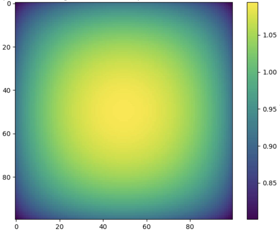
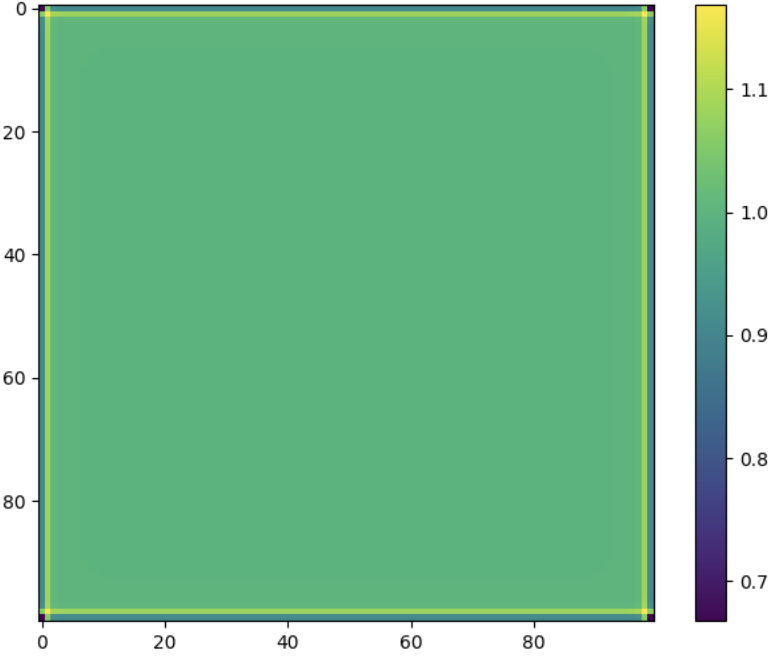
Figure 6. (left) Expected number of incoming shortcuts for $n=100$, and $\ell=q=1$. (right) Expected number of incoming shortcuts for $n=100,q=1$ and $\ell=5$.

Let $(G,o)\sim\mu$ be the random graph sampled according to $K(q,k,\ell)$ with measure $\mu$ defined in Section 3.5, and let $(G_{n},o_{n})=(K(n,q,k,\ell)\sim\mu_{n}$, $V(G_{n})$, $\mu_{r,n}$ and $\mu_{r}$ be defined as in the proof of Theorem 3.3. (Notice that we omitted $\epsilon$ here since the limit graph $G$ is unmarked, so we take $G_{n}$ as an unmarked graph, and mark equivalences are not considered.) Again, as in the proof of Theorem 8.1, it suffices to prove

(25) $$\frac{1}{n^{2}}\sum_{o_{n}\in V(G_{n})}\mathbbm{1}_{r}\big{(}(G_{n},o_{n})\simeq H_{*}\big{)}\overset{\mathbb{P}}{\to}\mu\Big{(}\mathbbm{1}_{r}\big{(}(G,o)\simeq H_{*})\big{)}\Big{)}\quad\text{ as $n\to\infty.$}$$

for all $r>0$ and $H_{*}=B_{r}(H_{*},o_{*})$ such that $\mu_{r}(H_{*},o_{*})>0$.

We will start with some definitions and preliminaries. Recall that we use $d(u,v)$ to denote the lattice distance between nodes, i.e. $d(u,v)=|x_{u}-x_{v}|+|y_{u}-y_{v}|$, and $d_{G}(u,v)$ to denote the graph distance between the nodes in graph $G$. Armed with these two definitions of distances, we can work with two types of local neighborhoods: graph neighborhoods given by $B_{r}(G,o)$ for a graph $G$ with root $o$ and lattice neighborhoods defined next.

Definition 9.1 (Lattice Neighborhood).

Let $L_{r}(G,o)$ denote the subgraph of $(G,o)$ induced by all the nodes $v\in V(G)$ whose lattice distance to $u$ is less than or equal to $r$:

$$L_{r}(G,o)=\{v\in V(G)|d(v,o)\leq r\}.$$

The following lemma shows that all shortcuts of a node span a short range, explaining why, in the limit, traversing through shortcuts does not change the marks.

Lemma 9.2.

Let $\psi:\mathbb{N}\to\mathbb{R}$ be a function that $\psi(n)\to\infty$ as $n\to\infty$, also let $G_{n}=K(n,q,k,\ell)$, where $\ell>2$. Then for a given vertex $u\in V(G_{n})$

$$\mathbbm{P}[\text{There exists a shortcut between $u$ and a node $v$ s.t. }d(u,v)>\psi(n)]\to 0\qquad\text{ as }n\to\infty.$$

Proof.

First, we bound the probability that there exists an incoming shortcut of distance at most $\psi(n)$. Let $S_{u}$ be the event that there exists an incoming shortcut to $u$ from a node $v$ such that $d(u,v)>\psi(n)$. There are at most $4mq$ nodes whose lattice distance from $u$ is $m$. Then, using union bound

$$\mathbbm{P}[S_{u}] \leq 4mq\sum_{j=\psi(n)+1}^{2n-2}j^{1-\ell}\quad\text{by applying an upper bound for \eqref{center}}$$

$$\leq 4mq\frac{\psi(n)^{2-\ell}-(2n-1)^{2-\ell}}{\ell-2}\quad\text{using}\int j^{1-\ell}dj=\frac{j^{2-\ell}}{2-\ell}$$

$$\to 0\quad\text{as $n\to\infty$. }$$

Now turning our attention to outgoing shortcuts, we have the following inequality from [30]: Let $u$ and $v$ be the two ends of a short-cut Then,

(26) $$\mathbbm{P}[d(u,v)>d]\leq 4(\ell-2)^{-1}d^{2-\ell}.$$

This gives that

$$\mathbbm{P}[\text{an outgoing shortcut of $u$ is to a node $v$ s.t. }d(u,v)>\psi(n)]\leq q(\ell-2)^{-1}\psi(n)^{2-\ell}\to 0$$

for any function $\psi(n)\to\infty$, proving the desired result. ∎

Lemma 9.2 shows that the shortcuts of a given node are contained within the $o(n)$ lattice neighborhood of it. Therefore, the marks of all nodes in $B_{r}(G_{n},o_{n})$––the coordinates normalized by $n$––will have the same mark as the mark of node $o_{n}$ for any finite $r$ in the limit.

We will later show a stronger result: for any $r$, there exists a constant $R$ such that, with high probability, the $R$-lattice neighborhood contains the $r$-graph neighborhood, i.e., $B_{r}(G_{n},v)\subseteq L_{R}(G_{n},v)$. This result is particularly useful because the $R$-lattice neighborhood of two nodes in $G_{n}$ are isomorphic if their distance to the boundary of the grid is larger than $R$. Consequently, for two uniformly chosen nodes $o_{1}$ and $o_{2}$ in $G_{n}$, their $R$-lattice neighborhoods are isomorphic with high probability, as the probability of sampling a node within the $R$ distance of the boundary tends to zero. As a result, the neighborhood structures of $B_{r}(G_{n},o_{1})$ and $B_{r}(G_{n},o_{2})$ have the same distribution (ignoring the marks) (see Figure 6-right panel). This conveniently eliminates the need for marks in the limiting graph.

With this, we are ready to prove (25) formally by proving the following two steps:

• The lattice neighborhood of $K(n,q,k,\ell)$ converges in probability to the lattice neighborhood of $K(q,k,\ell)$. We will use a Second-Moment argument here similar to the prior proofs.

• The lattice neighborhood convergence implies graph neighborhood convergence. For this purpose, we will use a careful path counting and coupling argument here inspired by [44].

To do so, we introduce the following notation:

$$\mathbbm{1}_{r}^{L}\big{(}(G_{n},o_{n})\simeq(H_{*},o_{*})\big{)}=\mathbbm{1}\Big{(}L_{r}(G_{n},o_{n})\simeq(H_{*},o_{*})\Big{)}.$$

Similar to the definition of expectation over $\mu$ and $\mu_{n}$, we will define $\mu_{r}^{L}((G,o)\simeq(H_{*},o_{*}))$ to be the probability of the event $L_{r}(G,o)\simeq(H_{*},o_{*})$ under measure $\mu$ and $\mu_{n,r}^{L}((G_{n},o_{n})\simeq(H_{*},o_{*}))$ to be the probability of the event $L_{r}(G_{n},o_{n})\simeq(H_{*},o_{*})$ under measure $\mu_{n}$.

9.1. Local Lattice Convergence

Lemma 9.3 (Lattice Neighborhood Convergence of Kleinberg Model).

Let $r>0$ be a constant. Then for any rooted graph $(H_{*},o_{*})$,

$$\frac{1}{n^{2}}\sum_{o_{n}\in V(G_{n})}\mathbbm{1}_{r}^{L}((G_{n},o_{n})\simeq(H_{*},o_{*}))\overset{\mathbb{P}}{\to}\mu_{r}^{L}((G,o)\simeq(H_{*},o_{*}))\quad\text{ as $n\to\infty.$}$$

Again, we will use the Second Moment Method to prove the convergence formally via the next two lemmas whose proofs are in Appendix B.

Lemma 9.4 (First Moment of Lattice Convergence).

Let $r>0$ be a constant. For any rooted graph $(H_{*},o_{*})$,

$$\mu_{r,n}^{L}((G_{n},o_{n})\simeq(H_{*},o_{*}))\to\mu_{r}^{L}((G,o)\simeq(H_{*},o_{*}))\quad\text{ as $n\to\infty.$}$$

Lemma 9.5 (Second Moment of Lattice Convergence).

Let $r>0$ be a constant. For any given rooted graph $(H_{*},o_{*})$,

$$\text{Var}\left(\frac{1}{n^{2}}\sum_{o_{n}\in V(G_{n})}\mathbbm{1}_{r}^{L}((G_{n},o_{n})\simeq(H_{*},o_{*}))\right)\to 0\quad\text{ as $n\to\infty.$}$$

Proof.

Given Lemma 9.4 and 9.5, the proof of Lemma 9.3 is identical to the proof of Lemma 7.1. ∎

9.2. Lattice Neighborhood Convergence implies Graph Neighborhood Convergence

Our goal in this section is to show that convergence of lattice neighborhoods implies convergence of graph neighborhood, i.e., Lemma 9.3 implies (25). For this purpose, it is enough to demonstrate that for any constant $r>0$, there exists a corresponding constant $R>0$ such that the lattice neighborhood of radius $R$ fully contains the graph neighborhood of radius $r$. The main idea behind the proof is to show that any path of a given length remains confined within a bounded distance in the lattice.

To establish this result, we adapt a technical lemma from [44], originally developed to analyze local limits of geometric random graphs. This adaptation allows us to rigorously account for the interplay between path lengths and lattice geometry within the context of the Kleinberg model.

For this purpose, we need the following notation. Given a path of shortcuts $\mathcal{U}_{n}=(o_{n}=u_{0},u_{1},u_{2},\cdots,u_{j-1})$ in $G_{n}$, and a path $\mathcal{U}=(o=u_{0},u_{1},u_{2},\cdots,u_{j-1})$ in $G$, let $P(G_{n},\mathcal{U}_{n})$ and $P(G,\mathcal{U})$ be the probabilities that path $\mathcal{U}_{n}$ exists in graph $G_{n}$ and path $\mathcal{U}$ exists in $G$, respectively.

Lemma 9.6 (Path Counting).

Given $\ell>2$, let $G_{n}=K(n,q,k,\ell)$ and $(G,o)\sim K(q,k,\ell)$, for any $j\geq 1$, and $a>1$,

(27) $$\lim_{b\to\infty}\limsup_{n\to\infty}\frac{1}{n^{2}}\sum_{u_{0},\ldots,u_{j}\in V(G_{n})}P(G_{n},u)\left(\prod_{i=0}^{j-2}\mathbbm{1}\left(d(u_{i+1},u_{i})\leq a^{b^{i+1}}\right)\right)\mathbbm{1}\left(d(u_{j},u_{j-1})>a^{b^{j}}\right)=0,$$

and

(28) $$\lim_{b\to\infty}\sum_{u_{0},\ldots,u_{j}\in L_{r}(G,o)}P(G,u)\left(\prod_{i=0}^{j-2}\mathbbm{1}\left(d(u_{i+1},u_{i})\leq a^{b^{i+1}}\right)\right)\mathbbm{1}\left(d(u_{j},u_{j-1})>a^{b^{j}}\right)=0,$$

where $r=r(a,b,j)=a^{b}+a^{b^{2}}+a^{b^{3}}+\cdots+a^{b^{j}}$.

As a corollary of this lemma, we will show for any fixed $K\in\mathbb{N}$ and $a,b>1$, if we choose $r=r(a,b,K)$ then the $K$-neighborhood of the rooted graph $L_{r}(G_{n},o_{n})$, and $B_{K}(G_{n},o_{n})$ will be the same in the limit as first $n$ and then $b\to\infty$, and the same result would hold for $(G,o)$. This is formalized in the following lemma, whose proof appears in the Appendix B.

Lemma 9.7 (Coupling Lattice Neighborhood with Graph Neighborhood).

Take any $K>0$ and $a,b>1$, and let $r=r(a,b,K)=a^{b}+a^{b^{2}}+a^{b^{3}}+\cdots+a^{b^{K}}$. Then,

(29) $$\lim_{b\to\infty}\limsup_{n\to\infty}\mu_{n,K}((L_{r}(G_{n},o_{n}),o_{n})\not\simeq B_{K}(G_{n},o_{n}))=0,$$

and

(30) $$\lim_{b\to\infty}\mu_{K}((L_{r}(G,o),o)\not\simeq B_{K}(G,o))=0.$$

Now, using Lemma 9.3 and Lemma 9.7, we will show that the lattice neighborhood convergence implies graph neighborhood convergence and, as a result, prove the main local convergence result in (25) and Theorem 3.5.

Proof of Theorem 3.5.

The proof closely follows the approach used for Theorem 1.11 in [44]. We provide a brief sketch of the proof and only go to the details of the main differences.

Fix some $a,b,K>1$ and let $r=r(a,b,K)=a^{b}+a^{b^{2}}+a^{b^{3}}+\cdots+a^{b^{K}}$. Note that $\frac{1}{n^{2}}\sum_{o_{n}\in V(G_{n})}\mathbbm{1}_{K}((G_{n},o_{n})\simeq H_{*})$ can be rewritten as

(31) $$\begin{split}&\frac{1}{n^{2}}\sum_{o_{n}\in V(G_{n})}\mathbbm{1}_{K}((G_{n},o_{n})\simeq H_{*})\mathbbm{1}_{K}((L_{r}(G_{n},o_{n}),o_{n})\simeq B_{K}(G_{n},o_{n}))\\ &+\frac{1}{n^{2}}\sum_{o_{n}\in V(G_{n})}\mathbbm{1}_{K}((G_{n},o_{n})\simeq H_{*})\mathbbm{1}_{K}((L_{r}(G_{n},o_{n}),o_{n})\not\simeq B_{K}(G_{n},o_{n})).\end{split}$$

Notice that the first term in (31) is

$$\frac{1}{n^{2}}\sum_{o_{n}\in V(G_{n})}\mathbbm{1}_{K}((L_{r}(G_{n},o_{n}),o_{n})\simeq H_{*})-\mathbbm{1}_{K}((L_{r}(G_{n},o_{n}),o_{n})\simeq H_{*})\mathbbm{1}_{K}((L_{r}(G_{n},o_{n}),o_{n})\not\simeq B_{K}(G_{n},o_{n})).$$

Let $\epsilon_{r,n}$ be

(32) $$\frac{1}{n^{2}}\sum_{o_{n}\in V(G_{n})}\mathbbm{1}_{K}((L_{r}(G_{n},o_{n}),o_{n})\not\simeq B_{K}(G_{n},o_{n}))\left[\mathbbm{1}_{K}((G_{n},o_{n})\simeq H_{*})-\mathbbm{1}_{K}((L_{r}(G_{n},o_{n}),o_{n})\simeq H_{*})\right]$$

giving

$$\frac{1}{n^{2}}\sum_{o_{n}\in V(G_{n})}\mathbbm{1}_{K}((G_{n},o_{n})\simeq H_{*})=\epsilon_{r,n}+\frac{1}{n^{2}}\sum_{o_{n}\in V(G_{n})}\mathbbm{1}_{K}((L_{r}(G_{n},o_{n}),o_{n})\simeq H_{*}).$$

We know that

$$0\leq\lim_{b\to\infty}\lim_{n\to\infty}\mathbbm{E}[|\epsilon_{n,K}|]\leq\lim_{b\to\infty}\lim_{n\to\infty}2\mu_{n,K}((L_{r}(G_{n},o_{n}),o_{n})\not\simeq B_{K}(G_{n},o_{n}))=0$$

by (32) and Lemma 9.7. Then, for any $\epsilon>0$, $K>0$, and $H_{*}=B_{K}(H_{*},o_{*})$, there exists large enough $m$ and $n$ such that

$$\mathbb{P}\left[\left|\frac{1}{n^{2}}\sum_{o_{n}\in V(G_{n})}\mathbbm{1}_{K}((G_{n},o_{n})\simeq H_{*})-\mathbbm{1}_{K}((L_{r}(G_{n},o_{n}),o_{n})\simeq H_{*})\right|>\epsilon\right]=\mathbb{P}[|\epsilon_{n,K}|>\epsilon]<\epsilon.$$

This gives $\frac{1}{n^{2}}\sum_{o_{n}\in V(G_{n})}\mathbbm{1}_{K}((G_{n},o_{n})\simeq H_{*})\overset{\mathbb{P}}{\to}\frac{1}{n^{2}}\sum_{o_{n}\in V(G_{n})}\mathbbm{1}_{K}((L_{r}(G_{n},o_{n}),o_{n})\simeq H_{*})$. By a similar argument, for any $\epsilon>0$, $K>0$, and $H_{*}=B_{K}(H_{*},o_{*})$, there exists large enough $m$ such that

$$\mathbb{P}\left[\left|\mu_{K}((G,o)\simeq H_{*})-\mu_{K}((L_{r}(G,o),o)\simeq H_{*})\right|>\epsilon\right]<\epsilon$$

and $\mu_{K}((G,o)\simeq H_{*})\overset{\mathbb{P}}{\to}\mu_{K}((L_{r}(G,o),o)\simeq H_{*})$. Together with Lemma 9.3, this completes the proof (25) and Theorem 3.5. ∎

10. Concluding Remarks

In this work, we established the local convergence of two foundational small-world network models—the Watts-Strogatz model and the Kleinberg model—providing theoretical insights into their asymptotic structures. For the Watts-Strogatz model, we characterized the local limit as the $k$-fuzz structure, demonstrating how rewiring induces a recursive process that preserves small-world properties while creating locally tree-like global structures. For the Kleinberg model, we showed a phase transition in the local limit at $\ell=2$, where the graph exhibits distinct behaviors depending on the decay of shortcut probabilities.

Our results unify the analysis of these models through the framework of local convergence and highlight their implications for global network properties, such as clustering coefficients, PageRank distributions, and the performance of decentralized search algorithms. By leveraging local limits, we provide a comprehensive foundation for studying small-world networks, offering tools for analyzing both graph properties and dynamic processes on these graphs.

Appendix A Second Moment: Proof of Lemma 8.3

For the second moment, we would like to show that

(33) $$\begin{split}&\lim_{n\to\infty}\text{Var}\left(\frac{1}{n^{2}}\sum_{o_{n}\in V(G_{n})}\mathbbm{1}_{r}^{\epsilon}((G_{n},o_{n})\simeq H_{*})\right)\\ &=\mathbb{E}\left[\left(\frac{1}{n^{2}}\sum_{o_{n}\in V(G_{n})}\mathbbm{1}_{r}^{\epsilon}((G_{n},o_{n})\simeq H_{*})\right)^{2}\right]-\mathbb{E}\left[\frac{1}{n^{2}}\sum_{o_{n}\in V(G_{n})}\mathbbm{1}_{r}^{\epsilon}((G_{n},o_{n})\simeq H_{*})\right]^{2}\to 0.\end{split}$$

We will follow the same steps as the proof for the second moment for the Watts-Strogatz model (Lemma 7.3). The only difference is that instead of summing over all nodes, we need to sum over a subset of nodes because we need mark differences to be at most $\epsilon$. To do so, let’s define $W_{\epsilon,m}=\left\{w\in V(G_{n})\big{|}\left\|m-M(w)\right\|_{1}<\epsilon\right\}$, where $M(w)$ is mark of node $w$, for any $\epsilon>0$ and $m\in M$. Let the mark of the root of $H_{*}$ be $M(v_{0,*})$. By linearity of expectation,

(34) $$\begin{split}&\lim_{n\to\infty}\mathbb{E}\left[\left(\frac{1}{n^{2}}\sum_{o_{n}\in V(G_{n})}\mathbbm{1}_{r}^{\epsilon}((G_{n},o_{n})\simeq H_{*})\right)^{2}\right]\\ &=\lim_{n\to\infty}\frac{1}{n^{4}}\sum_{v_{0}\in W_{\epsilon,m_{*}}}\sum_{\begin{subarray}{c}w_{0}\in W_{\epsilon,M(v_{0,*})}\\ w_{0}\neq v_{0}\end{subarray}}\mathbbm{P}\left[B_{r}(G_{n},v_{0})\simeq H_{*}\right]\mathbbm{P}\left[B_{r}(G_{n},w_{0})\simeq H_{*}|B_{r}(G_{n},v_{0})\simeq H_{*}\right]\\ &\to\lim_{n\to\infty}\frac{1}{n^{2}}\sum_{v_{0}\in W_{\epsilon,m_{*}}}\frac{|W_{\epsilon,M(v_{0,*})}|-1}{n^{2}}\quad\mathbbm{P}\left[B_{r}(G_{n},v_{0})\simeq H_{*}\right]\mathbbm{P}_{w_{0}}\left[B_{r}(G_{n},w_{0})\simeq H_{*}|B_{r}(G_{n},v_{0})\simeq H_{*}\right]\end{split}$$

where the first probability $\mathbbm{P}$ is over the randomness of $G_{n}$ but $\mathbbm{P}_{w_{0}}$ is also over the randomness of root $w_{0}$ that is sampled uniformly at random from $W_{\epsilon,M(v_{0,*})}\backslash\{v_{0}\}$. Since $|W_{\epsilon,m}|\geq\sum_{j=1}^{\lfloor\epsilon n-1\rfloor}j=\frac{1}{2}\epsilon n(\epsilon n-1)$,

$$\mathbbm{P}_{w_{0}}[w_{0}\notin B_{2r}(G_{n},v_{0})]\geq 1-\frac{\mathbbm{E}[|B_{2r}(G_{n},v_{0})]|}{\frac{1}{2}\epsilon^{2}n^{2}}\to 1\quad\text{ as $n\to\infty$}$$

by Lemma 6.4. Since $B_{r}(G_{n},w_{0})$ has finitely many shortcuts almost surely, none of them will connect to the finite set $B_{2r}(G_{n},v_{0})$ with high probability by Lemma 8.4. This implies $B_{r}(G_{n},w_{0})\cap B_{2r}(G_{n},v_{0})=\emptyset$ holds with high probability. Then,

$$\lim_{n\to\infty}\mathbbm{P}_{w_{0}}\left[B_{r}(G_{n},w_{0})\simeq H_{*}|B_{r}(G_{n},v_{0})\simeq H_{*}\right]$$

is the same as

$$\lim_{n\to\infty}\mathbbm{P}_{w_{0}}\left[B_{r}(G_{n},w_{0})\simeq H_{*}\big{|}B_{r}(G_{n},v_{0})\simeq H_{*}\text{ and }B_{r}(G_{n},w_{0})\cap B_{r}(G_{n},v_{0})=\emptyset\right].$$

Finally, we have the following lemma giving the conditional independence of the events.

Lemma A.1.

Let B be the event that $\big{(}B_{r}(G_{n},v_{0})\simeq H_{*}\big{)}\cap\big{(}B_{r}(G_{n},w_{0})\cap B_{r}(G_{n},v_{0})=\emptyset\big{)}$. Then,

(35) $$\lim_{n\to\infty}\mathbbm{P}_{w_{0}}\left[B_{r}(G_{n},w_{0})\simeq H_{*}\big{|}\text{{B}}\right]=\lim_{n\to\infty}\mathbbm{P}_{w_{0}}\left[B_{r}(G_{n},w_{0})\simeq H_{*}\right]$$

Assuming Lemma A.1, the proof of Lemma 8.3 follows from (33) and (34). ∎

Proof of Lemma A.1

Let $v_{i,n}$ and $v_{i,*}$ be $i$-th node in $(\overline{G}_{n},w_{0})$ and $\overline{H_{*}}$ respectively, $M(v_{i,n})$ and $M(v_{i,*})$ be their corresponding marks, and $x_{i}$ is the number of incoming shortcuts of $v_{i,*}$. Finally, define $T_{i}$ be the event that $(\overline{G}_{n},w_{0})$ and $H_{*}$ look identical up until $i$-th node in the BFS. We can write the right-hand-side of (35) as the limit of

$$\prod_{i\in[\overline{H_{*}}]}\mathbbm{P}[\text{$v_{i,n}$ has $x_{i}$ incoming shortcuts}|M(v_{i,n})=M(v_{i,*}),T_{i-1}]\mathbbm{P}[M(v_{i,n})=M(v_{i,*})|T_{i-1}],$$

similar to (15), and the left-hand side similarly where each probability would additionally be conditioned on B.

Since $\overline{H_{*}}$ is a finite graph, to prove Lemma A.1, it suffices to prove the following two statements:

(36) $$\lim_{n\to\infty}\mathbbm{P}[M(v_{i,n})=M(v_{i,*})|T_{i-1}\text{ and {B}}]=\lim_{n\to\infty}\mathbbm{P}[M(v_{i,n})=M(v_{i,*})|T_{i-1}],$$

and

(37) $$\begin{split}&\lim_{n\to\infty}\mathbbm{P}[\text{$v_{i,n}$ has $x_{i}$ incoming shortcuts}|M(v_{i,n})=M(v_{i,*}),T_{i-1},\text{ and {B}}]\\ &=\lim_{n\to\infty}\mathbbm{P}[\text{$v_{i,n}$ has $x_{i}$ incoming shortcuts}|M(v_{i,n})=M(v_{i,*}),T_{i-1}].\end{split}$$

Let’s start with (36). We are going to rely on parts of the proof for Lemma 8.9, so we will only mention the important differences. We have two types of shortcuts, giving two cases. Case 1: $v_{i,x}$ is explored through an outgoing shortcut. By the same logic as (18), left-hand side of (36) is greater than

$$\lim_{n\to\infty}\frac{[d(v_{p(i),n},v_{i,n})]^{-\ell}}{\sum_{u\notin\{v_{i,n}\}\cup B_{r}(G_{n},v_{0})}[d(v_{i,n},u)]^{-\ell}}-o(1),$$

and less than

$$\lim_{n\to\infty}\frac{[d(v_{p(i),n},v_{i,n})]^{-\ell}}{\sum_{u\notin\{v_{i,n}\}\cup B_{2r}(G_{n},v_{0})}[d(v_{i,n},u)]^{-\ell}}+o(1),$$

both of which converges to

$$\lim_{n\to\infty}\frac{[d(v_{p(i),n},v_{i,n})]^{-\ell}}{\sum_{u\neq v_{i,n}}[d(v_{i,n},u)]^{-\ell}}$$

since $q\sum_{u\in\cup B_{2r}(G_{n},v_{0})}[d(v_{i,n},u)]^{-\ell}=o\left(q\sum_{u\neq v_{i,n}}[d(v_{i,n},u)]^{-\ell}\right)$ by Lemma 6.4. By (18), (36) follows for the first case. Case 2: $v_{i,x}$ is explored through an incoming shortcut. A similar argument relying on (19) will show that the left-hand side of (36) converges to

$$\lim_{n\to\infty}\frac{[d(v_{p(i),n},v_{i,n})]^{-\ell}}{q\sum_{u\neq v_{i,n}}[d(v_{i,n},u)]^{-\ell}},$$

proving (36) for the second case as well.

Next, we move to identity (37). Again, we are going to rely on parts of the proof for Lemma 8.10, so we will only mention the important differences. Similar to Lemma 8.10, define $\text{{S}}_{i}$ to be the set of ordered $x_{i}$ shortcuts that can feasibly serve as incoming shortcuts for $v_{i,n}$ given $M(v_{i,n})=M(v_{i,*})$, $T_{i-1}$ and B. We would have the following identity:

$$\{(s_{1},\cdots,s_{x_{i}})|\text{{Out}}_{s_{j},i}<q,s_{j}\notin B_{2r}(G_{n},v_{0})\text{ for all }1\leq j\leq x_{i}\text{ and }s_{i}\neq s_{j}\text{ for any }i\neq j\}\subseteq\text{{S}}_{i}.$$

Then, the left-hand-side of (37) can be written as

$$\lim_{n\to\infty}\sum_{(s_{1},\cdots,s_{x_{i}})\in\text{{S}}_{i}}\prod_{j=1}^{x_{i}}\frac{[d(s_{j},v_{i,n})]^{-\ell}}{\sum_{v}[d(s_{j},v)]^{-\ell}}\prod_{u}\left(1-\frac{[d(u,v_{i,n})]^{-\ell}}{\sum_{v}[d(u,v)]^{-\ell}}\right)^{q-\text{{Out}}_{u,i}}\prod_{j=1}^{x_{i}}\frac{1}{1-\frac{[d(s_{j},v_{i,n})]^{-\ell}}{\sum_{v}[d(s_{j},v)]^{-\ell}}},$$

similar to (20). Then, one can follow the same steps as the proof for Lemma 8.10 and rely on Lemma 6.2 and 6.4 to bound $\sum_{u}\text{{Out}}_{u,i}+q|B_{2r}(G_{n},v_{0})|$ and conclude (22) here too.

To conclude (23), recall the definition of $\text{{E}}_{i}$ from the proof for Lemma 8.10 and consider $\text{{E}}_{i}\cup B_{2r}(G_{n},v_{0})$. Again, following the proof for Lemma 8.10 and relying on Lemma 6.2 and 6.4 to bound $|\text{{E}}_{i}\cup B_{2r}(G_{n},v_{0})|$, the conclusion follows. ∎

Appendix B Omitted Proofs from Section 9

Proof of Lemma 9.4

Suppose $(H_{*},o_{*})$ is a sample from $\mu_{r}^{L}$ such that $\mu_{r}^{L}(H_{*},o_{*})>0$, i.e., it can be sampled with positive probability. We will order the nodes in $L_{r}(G_{n},o)$, $L_{r}(G,o)$ and $L_{r}(H_{*},o_{*})$ such that the nodes with smaller $y$ coordinates take precedence over others and ties are broken by giving precedence to nodes with smaller $x$ coordinates. The first node in this ordering would be the top-left node. Notice that this naturally gives an ordering of each shortcut: the shortcut that connects nodes with a smaller sum of orders takes precedence. Let $L_{r}(\overline{G}_{n},o)$, $L_{r}(\overline{G},o)$, and $\overline{H_{*}}=L_{r}(\overline{H_{*}},o_{*})$ be the ordered versions. Note that this ordering changes depending on $r$ for $G$ and $H_{*}$ and is based on both $o_{n}$ and $r$ for $G_{n}$. As in the case of the Watts-Strogatz model, for the first moment, it suffices to prove that

$$\mu_{r,n}^{L}((\overline{G_{n}},o_{n})=\overline{H_{*}})\to\mu_{r}^{L}((\overline{G},o)=\overline{H_{*}}).$$

The lattice connections in $L_{r}(G,o)$, and $L_{r}(H_{*},o_{*})$ are formed following the same procedure by definition. For the finite case, as long as the distance of $o_{n}$ to the boundary is at least $r$, the lattice connections observed in $L_{r}(G_{n},o)$ and $L_{r}(H_{*},o_{*})$ are the same too. This happens with high probability since $1-\frac{r^{2}}{n^{2}}\to 1$. Hence, from now on, we will assume all lattice connections will be the same. Given that $o_{n}$ is distant enough for this to hold, we will now explore the outgoing shortcuts of each node in $L_{r}(G_{n},o)$ following the ordering to give a closed form for $\mu_{r,n}^{L}((\overline{G_{n}},o_{n})=\overline{H_{*}})$.

Let’s say $v_{i}$ is the $i$-th node in $L_{r}(\overline{G}_{n},o)$, $x_{i}$ is the number of outgoing shortcuts of $i$-th node in $L_{r}(\overline{H_{*}},o_{*})$ that connects to one of the nodes in $L_{r}(H_{*},o_{*})$, and $d_{i,j}$ is the distance of $j^{th}$ shortcut of $i^{th}$ node in $L_{r}(H_{*},o_{*})$. Now, recall that the probability that an outgoing shortcut of $v$ connects to $w$ is $\frac{[d(v,w)]^{-\ell}}{4\zeta(\ell-1)}$ in $G$ and $\frac{[d(v,w)]^{-\ell}}{D_{v}^{(n)}}$ in $G_{n}$ where $D_{v}^{(n)}=\sum_{\begin{subarray}{c}u\neq v\\ u\in V(G_{n})\end{subarray}}d(v,u)^{-\ell}$. Then, by independence of each outgoing shortcut,

(38) $$\mu_{r,n}^{L}((\overline{G_{n}},o_{n})=\overline{H_{*}})=\prod_{i\in[\overline{H_{*}}]}\binom{q}{x_{i}} \left(\frac{\sum_{\begin{subarray}{c}w\neq v_{i}\\ w\in V(L_{r}(G_{n},o_{n}))\end{subarray}}[d(v_{i},w)]^{-\ell}}{D_{v_{i}}^{(n)}}\right)^{x_{i}}$$

(39) $$\prod_{j=1}^{x_{i}}\frac{d_{i,j}^{-\ell}}{\sum_{\begin{subarray}{c}w\neq v_{i}\\ w\in V(L_{r}(G_{n},o_{n}))\end{subarray}}[d(v_{i},w)]^{-\ell}}.$$

(40) $$\quad\left(1-\frac{\sum_{\begin{subarray}{c}w\neq v_{i}\\ w\in V(L_{r}(G_{n},o_{n}))\end{subarray}}[d(v_{i},w)]^{-\ell}}{D_{v_{i}}^{(n)}}\right)$$

where $u_{0}=o_{n}$ is uniformly chosen from all the nodes with a distance at least $r$ to the boundary. Here, $\binom{q}{x_{i}}$ gives the number of ways of choosing $x_{i}$ shortcuts out of $q$ outgoing shortcuts of a node to be connected $L_{r}(G_{n},o_{n})$, the fraction in (38) gives the probability that these $x_{i}$ outgoing shortcuts connect to nodes in $L_{r}(G_{n},o_{n})$, the product in (39) gives the probability that each of $x_{i}$ shortcuts connects to a specific node in $L_{r}(G_{n},o_{n})$ given that they are connecting to $L_{r}(G_{n},o_{n})$, and, lastly, (40) gives the probability that the rest connects to nodes outside of $L_{r}(G_{n},o_{n})$.

On the other hand, the closed form for $\mu_{r}^{L}((\overline{G},o)=(\overline{H_{*}},o_{*}))$ is the same as above except $L_{r}(G_{n},o_{n})$ is replaced with $L_{r}(G,o)$ and all $D_{u_{i}}^{(n)}$’s are replaced with $4\zeta(\ell-1)$. Then, since $L_{r}(G_{n},o_{n})$ and $L_{r}(G,o)$ are finite almost surely, it suffices to show the following lemma to conclude the proof.

Lemma B.1.

Fix any $r>0$ and $\epsilon>0$. For a given node $v$, let $D_{v}^{(n)}=\sum_{\begin{subarray}{c}u\neq v\\ u\in V(G_{n})\end{subarray}}d(v,u)^{-\ell}$. Then,

$$\mathbbm{P}\left[\left|\frac{1}{D_{v_{i}}^{(n)}}-\frac{1}{4\zeta(\ell-1)}\right|\leq\epsilon\text{ for all }v_{i}\in V(L_{r}(G_{n},o_{n}))\right]\to 1$$

as $n\to\infty$ where the probability is over the uniform distribution of $o_{n}$ over all the nodes with a distance at least $r$ to the boundary of $G_{n}$.

Proof.

Take any $\epsilon>0$ and choose some $\delta<\frac{\epsilon 16\zeta(\ell-1)^{2}}{4+\epsilon 16\zeta(\ell-1)^{2}}$. We know for $\ell>2$, $\sum_{d=1}^{\infty}d^{1-\ell}=\zeta(\ell-1)$. Then, there is $R_{\delta}$ such that $\zeta(\ell-1)-\sum_{d=1}^{R_{\delta}}d^{1-\ell}\leq\delta.$ If a node $v$’s distance from the boundary is at least $R_{\delta}$, then

$$\sum_{\begin{subarray}{c}v\neq u\\ v\in V(G_{n})\end{subarray}}d(v,u)^{-\ell} \geq\sum_{\begin{subarray}{c}v\neq u\\ v\in B_{R_{\delta}}(u)\end{subarray}}d(v,u)^{-\ell}=4\sum_{d=1}^{R_{\delta}}d^{1-\ell}\geq 4\zeta(\ell-1)-4\delta.$$

On the other hand,

$$\sum_{\begin{subarray}{c}u\neq v\\ v\in V(G_{n})\end{subarray}}d(u,v)^{-\ell} \leq 4\sum_{d=1}^{n}d^{1-\ell}\leq 4\zeta(\ell-1).$$

Choose $\delta<\frac{\epsilon 16\zeta(\ell-1)^{2}}{4+\epsilon 16\zeta(\ell-1)^{2}}$ and assume $v_{i}$’s distance to the boundary is greater than $R_{\delta}$, then

$$\left|\frac{1}{D_{v_{i}}^{(n)}}-\frac{1}{4\zeta(\ell-1)}\right|\leq\frac{4\delta}{4\zeta(\ell-1)(4\zeta(\ell-1)-4\delta)}\leq\epsilon.$$

Notice

$$\left|\frac{1}{D_{u_{i}}^{(n)}}-\frac{1}{4\zeta(\ell-1)}\right|\leq\epsilon$$

is guaranteed happen for all $v_{i}\in V(L_{r}(G_{n},o_{n}))$ if $o_{n}$ is at least $2R_{\delta}$ far apart from the boundary. The probability of this event is at least

$$1-\frac{4R_{\delta}^{2}}{n^{2}}\to 1.$$

concluding the proof of this lemma. ∎

By taking a union bound over all nodes in $L_{r}(G_{n},o_{n})$ and applying the lemma above, we get the proof of first-moment for the $r$-lattice neighborhoods. ∎

Proof of Lemma 9.5

As the argument follows a similar structure to the second-moment proofs presented earlier, we provide a brief outline here, focusing on the key steps. We are interested in showing that

$$\lim_{n\to\infty}\Bigg{(}\mathbb{E}\Bigg{[}\Big{(}\frac{1}{n^{2}}\sum_{o_{n}\in V(G_{n})}\mathbbm{1}_{r}^{L}((G_{n},o_{n})\simeq H_{*})\Big{)}^{2}\Bigg{]}$$

$$\quad-\frac{1}{n^{4}}\sum_{v_{0},w_{0}\in V(G_{n}),d(v_{0},w_{0})>2r}\mathbbm{P}\left[L_{r}(G_{n},v_{0})\simeq H_{*}\right]\mathbbm{P}\left[L_{r}(G_{n},w_{0})\simeq H_{*}\right]\Bigg{)}=0.$$

First, note that when $L_{r}(G_{n},v_{0})\cap L_{r}(G_{n},w_{0})=\emptyset$, we have $L_{r}(G_{n},v_{0})\simeq H_{*}$ and $L_{r}(G_{n},w_{0})\simeq H_{*}$ are independent. So to prove the result, it is enough to show that

(41) $$\lim_{n\to\infty}\frac{1}{n^{4}}\sum_{v_{0},w_{0}\in V(G_{n}),d(v_{0},w_{0})<2r}\mathbbm{P}\left[L_{r}(G_{n},v_{0})\simeq H_{*},L_{r}(G_{n},w_{0})\simeq H_{*}\right]\Big{)}=0$$

Note that for any finite $r$, we know that $|L_{2r}(G_{n},v_{0})|$ is bounded by a constant $C$ independent of $n$. As a result, number of pairs that their $r$-lattice neighborhood overlap (i.e., $L_{r}(G_{n},v_{0})\cap L_{r}(G_{n},w_{0})\neq\emptyset$) is upper bounded by $Cn^{2}$. Since each probability is bounded by $1$, the sum of terms that appear in the left-hand side of (41) is at most $\frac{Cn^{2}}{n^{4}}$ which converges to zero as desired.

Now, one can follow the same steps as the ones in section 7 to conclude the proof. ∎

Proof of Lemma 9.6

Since the proof is very similar to the proof Lemma 3.3 in [44], we will be brief. By Fubini’s theorem for infinite series,

$$\lim_{b\to\infty}\lim_{n\to\infty}\sum_{u\in I_{n}^{j}}P(G_{n},u)\left(\prod_{i=1}^{j-1}\mathbbm{1}\left(\|u_{i+1}-u_{i}\|\leq a^{b^{i+1}}\right)\right)\mathbbm{1}\left(\|u_{j}-u_{j-1}\|>a^{m^{j-1}}\right)$$

$$\leq\lim_{b\to\infty}C_{1}(a^{b})^{2}\cdots(a^{b^{j}})^{2}\mathbbm{E}_{(u_{j-1},u_{j})\in I_{n}^{2}}\left[\mathbbm{1}\left(\|u_{j}-u_{j-1}\|>a^{b^{j}}\right)\right]$$

for some constant $$C_{1}$$, and

$$\leq\lim_{b\to\infty}C_{1}(a^{b})^{2}\cdots(a^{b^{j-1}})^{2}8q(\ell-2)^{-1}a^{b^{j}(2-\ell)}$$

by substituting $$d=a^{b^{j}} 2q C_{2}$$ to inequality (26) from [30], and taking union bound over at most shortcuts between any two nodes. Then, for some constant ,

$$\leq\lim_{b\to\infty}C_{2}a^{2b+\cdots+2b^{j-1}-b^{j}(\ell-2)}=0$$

for any $a>1$ and $\ell>2$. The proof for (28) is identical since the inequality given by (26) also works for the limiting graph $(G,o)$. ∎

Proof of Lemma 9.7

Since the proof is very similar to the proof Corollary 3.5 in [44], we will be brief. Take $r=r(a,b,K)=a^{b}+a^{b^{2}}+a^{b^{3}}+\cdots+a^{b^{K}}$ for some $a,b>1$. The event $\{B_{K}(L_{r}(G_{n},o_{n}),o_{n})\neq B_{K}(G_{n},o_{n})\}$ implies that there is some edge $(u_{i},u_{i+1})$ in $B_{K}(G_{n},o_{n})$ such that the lattice distance $d(u_{i},u_{i+1})>a^{b^{L+1}}$. Let’s call this event $\text{{Bad}}_{r,n}$ for $G_{n}$ and the corresponding event $\text{{Bad}}_{r}$ for $G$. Define

$$\mathcal{I}_{n,j}: =\{\exists u_{1},\dots,u_{j}\in V(G_{n})|\{u_{0},u_{1},\dots,u_{j}\}\text{ is a }j\text{-path in }(G_{n},o_{n})\text{ starting from }v_{0}=o_{n},$$

$$\forall 0\leq i\leq j-2,d(u_{i},u_{i+1})\leq a^{b^{j+1}},d(u_{j-1},u_{j})>a^{b^{j+1}}\}$$

and $\mathcal{I}_{j}$ is the corresponding event in $(G,o)$. Then, by union bound, we have

(42) $$\mu_{n}(B_{K}(L_{r}(G_{n},o_{n}),o_{n})\neq B_{K}(G_{n},o_{n}))\leq\mu_{n}(\text{{Bad}}_{r,n})\leq\sum_{j=1}^{K}\mathbbm{P}[\mathcal{I}_{n,j}]$$

and

(43) $$\mu(B_{K}(L_{r}(G,o),o)\neq B_{K}(G,o))\leq\mu(\text{{Bad}}_{r})\leq\sum_{j=1}^{K}\mathbbm{P}[\mathcal{I}_{j}].$$

Since $K$ is fixed, the probabilities on the right-hand side of (42) and (43) both tend to $0$ by Lemma 9.6. ∎

Appendix C Proof of Applications

Proof of Corollary 4.1

By Theorems 2.22 and 2.23 in [28], we know that the local clustering coefficient converges to $\mathbb{E}_{\mu}\left[\frac{\Delta_{G}(o)}{d_{o}(d_{o}-1)}\right]$ and global clustering coefficient converges to $\frac{\mathbb{E}_{\mu}[\Delta_{G}(o)]}{\mathbb{E}_{\mu}[d_{o}(d_{o}-1)]}$ where $\Delta_{G}(o)$ is twice the number of triangles that contains $o$. Since the graph follows a symmetric distribution $\mu$, the final expression for local clustering does not depend on $v$ and one can easily obtain from the limit for a given $k$. For global clustering, recall that the (outgoing or incoming) shortcuts in the limiting graph connect to different (full or reduced) $k$-fuzzes and, hence, cannot be part of a triangle (or any cycle for that matter). Thus, the triangles that contain any node can only be created by the non-rewired ring edges each of which exists with probability $1-\phi$. The degree of the root $d_{o}$ under $\mu$ is distributed according to $\text{Bin}(k,1-\phi)+\text{Bin}(k,\phi)+\text{Bin}(k,1-\phi)+\text{Poi}(\phi k)$ for outgoing ring edges, outgoing shortcuts, incoming ring edges, and incoming shortcuts respectively. Then,

$$\mathbb{E}[d_{o}^{2}-d_{0}]=\text{Var}(d_{o})+\mathbb{E}[d_{o}]^{2}-\mathbb{E}[d_{o}]=k(1-\phi)\phi+\phi k+4k^{2}-2k$$

and the twice number of triangles that contain some node in a Full $k$-Path is $3k(k-1)$. Each exists with probability $(1-\phi)^{3}$ after rewiring. Then, by linearity of expectation, we get

$$\frac{3k(k-1)(1-\phi)^{3}}{k(1-\phi)\phi+\phi k+4k^{2}-2k}=\frac{3(k-1)}{2(2k-1)+\phi(2-\phi)}(1-\phi)^{3}$$

as the final expression. ∎

Proof of Corollary 4.2

Again, since each shortcut connects to a different $k$-lattice when $\ell\leq 2$, shortcuts cannot create any triangle. Thus, the numerator is going to be the number of triangles containing any node in a $k$-lattice. By symmetry, this is the same for all nodes and is deterministic, so it can be taken out of expectation, making limits of both local and global clustering coefficients the same. Then, the randomness can only come from the degree of a node which depends on its mark $m$ sampled uniformly from $M=[0,1]\times[0,1]$. Since the incoming shortcut distribution is $\text{Poi}(\Lambda_{m})$ for each $m$ sampled uniformly from $M$, the number of outgoing shortcuts is $q$, and the number of lattice edges is $2k(k+1)$ almost surely, we have

$$\mathbb{E}[d_{o}^{2}-d_{0}]=\text{Var}(d_{o})+\mathbb{E}[d_{o}]^{2}-\mathbb{E}[d_{o}]=(2k(k+1)+q+\Lambda_{m})^{2}-(2k(k+1)+q),$$

and the conclusion follows. ∎

References

- [1] D. Aldous and J.M. Steele. The objective method: probabilistic combinatorial optimization and local weak convergence. In Probability on discrete structures, volume 110 of Encyclopaedia Math. Sci., pages 1–72. Springer, Berlin, 2004.
- [2] Yeganeh Alimohammadi, Christian Borgs, and Amin Saberi. Algorithms using local graph features to predict epidemics. In Proceedings of the 2022 Annual ACM-SIAM Symposium on Discrete Algorithms (SODA), pages 3430–3451. SIAM, 2022.
- [3] Yeganeh Alimohammadi, Christian Borgs, and Amin Saberi. Locality of random digraphs on expanders. The Annals of Probability, 51(4):1249 – 1297, 2023.
- [4] Yeganeh Alimohammadi, Christian Borgs, Remco van der Hofstad, and Amin Saberi. Epidemic forecasting on networks: Bridging local samples with global outcomes. Technical report, Technical report, Working paper, 2023.
- [5] A Barbour and G Reinert. Discrete small world networks. ELECTRONIC JOURNAL OF PROBABILITY, 11, 2006.
- [6] Marco Bardoscia, Paolo Barucca, Stefano Battiston, Fabio Caccioli, Giulio Cimini, Diego Garlaschelli, Fabio Saracco, Tiziano Squartini, and Guido Caldarelli. The physics of financial networks. Nature Reviews Physics, 3(7):490–507, 2021.
- [7] Alain Barrat and Martin Weigt. On the properties of small-world network models. The European Physical Journal B-Condensed Matter and Complex Systems, 13:547–560, 2000.
- [8] Danielle Smith Bassett and ED Bullmore. Small-world brain networks. The neuroscientist, 12(6):512–523, 2006.
- [9] Itai Benjamini and Noam Berger. The diameter of long-range percolation clusters on finite cycles. Random Structures & Algorithms, 19(2):102–111, 2001.
- [10] Itai Benjamini and Oded Schramm. Recurrence of distributional limits of finite planar graphs, 2001.
- [11] N. Berger, C. Borgs, J. Chayes, and A. Saberi. Asymptotic behavior and distributional limits of preferential attachment graphs. Annals of Probability, 42(1):1–40, 2014.
- [12] B. Bollobás, S. Janson, and O. Riordan. The phase transition in inhomogeneous random graphs. Random Structures Algorithms, 31(1):3–122, 2007.
- [13] Béla Bollobás, Svante Janson, and Oliver Riordan. Sparse random graphs with clustering. Random Structures & Algorithms, 38(3):269–323, 2011.
- [14] Charles Bordenave, Marc Lelarge, and Justin Salez. Matchings on infinite graphs. Probability Theory and Related Fields, 157:183–208, 2013.
- [15] Peer Bork, Lars J Jensen, Christian Von Mering, Arun K Ramani, Insuk Lee, and Edward M Marcotte. Protein interaction networks from yeast to human. Current opinion in structural biology, 14(3):292–299, 2004.
- [16] Andrei Broder, Ravi Kumar, Farzin Maghoul, Prabhakar Raghavan, Sridhar Rajagopalan, Raymie Stata, Andrew Tomkins, and Janet Wiener. Graph structure in the web. Computer networks, 33(1-6):309–320, 2000.
- [17] Don Coppersmith, David Gamarnik, and Maxim Sviridenko. The diameter of a long-range percolation graph. Random Structures & Algorithms, 21(1):1–13, 2002.
- [18] A. Dembo and A. Montanari. Gibbs measures and phase transitions on sparse random graphs. Braz. J. Probab. Stat., 24(2):137–211, 2010.
- [19] Martin Dietzfelbinger and Philipp Woelfel. Tight lower bounds for greedy routing in uniform small world rings. In Proceedings of the forty-first annual ACM symposium on Theory of computing, pages 591–600, 2009.
- [20] Martin E Dyer, Andreas Galanis, Leslie Ann Goldberg, Mark Jerrum, and Eric Vigoda. Random walks on small world networks. ACM Transactions on Algorithms (TALG), 16(3):1–33, 2020.
- [21] Abraham D. Flaxman. Expansion and lack thereof in randomly perturbed graphs. In William Aiello, Andrei Broder, Jeannette Janssen, and Evangelos Milios, editors, Algorithms and Models for the Web-Graph, pages 24–35, Berlin, Heidelberg, 2008. Springer Berlin Heidelberg.
- [22] Pierre Fraigniaud and George Giakkoupis. On the searchability of small-world networks with arbitrary underlying structure. In Proceedings of the forty-second ACM symposium on Theory of computing, pages 389–398, 2010.
- [23] David Gamarnik, Tomasz Nowicki, and Grzegorz Swirszcz. Maximum weight independent sets and matchings in sparse random graphs. exact results using the local weak convergence method. Random Structures & Algorithms, 28(1):76–106, 2006.
- [24] Ankan Ganguly and Kavita Ramanan. Hydrodynamic limits of non-markovian interacting particle systems on sparse graphs. arXiv preprint arXiv:2205.01587, 2022.
- [25] A. Garavaglia, R. Hazra, R. van der Hofstad, and R. Ray. Universality of the local limit in preferential attachment models. arXiv:2212.05551 [math.PR], 2022.
- [26] Alessandro Garavaglia, Remco van der Hofstad, and Nelly Litvak. Local weak convergence for pagerank. The Annals of Applied Probability, 30(1):pp. 40–79, 2020.
- [27] George Giakkoupis and Nicolas Schabanel. Optimal path search in small worlds: dimension matters. In Proceedings of the forty-third annual ACM symposium on Theory of computing, pages 393–402, 2011.
- [28] Remco van der Hofstad. Random graphs and complex networks. Cambridge Series in Statistical and Probabilistic Mathematics, 1, 2016.
- [29] Mark D Humphries, Kevin Gurney, and Tony J Prescott. The brainstem reticular formation is a small-world, not scale-free, network. Proceedings of the Royal Society B: Biological Sciences, 273(1585):503–511, 2006.
- [30] Jon Kleinberg. The small-world phenomenon: an algorithmic perspective. In Proceedings of the Thirty-Second Annual ACM Symposium on Theory of Computing, STOC ’00, page 163–170, New York, NY, USA, 2000. Association for Computing Machinery.
- [31] JK̇omjáthy and B. Lodewijks. Explosion in weighted hyperbolic random graphs and geometric inhomogeneous random graphs. Stochastic Process. Appl., 130(3):1309–1367, 2020.
- [32] D. Krioukov, F. Papadopoulos, M. Kitsak, A. Vahdat, and M. Boguñá. Hyperbolic geometry of complex networks. Phys. Rev. E (3), 82(3):036106, 18, 2010.
- [33] Santanu Kundu and Santanu Chattopadhyay. Network-on-chip: the next generation of system-on-chip integration. Taylor & Francis, 2014.
- [34] V. Kurauskas. On local weak limit and subgraph counts for sparse random graphs. Journal of Applied Probability, 59(3):755–776, 2022.
- [35] Daniel Lacker, Kavita Ramanan, and Ruoyu Wu. Local weak convergence for sparse networks of interacting processes. arXiv preprint arXiv:1904.02585, 2019.
- [36] Mattia Mattei, Manuel Pratelli, Guido Caldarelli, Marinella Petrocchi, and Fabio Saracco. Bow-tie structures of twitter discursive communities. Scientific Reports, 12(1):12944, 2022.
- [37] Abbas Mehrabian and Ali Pourmiri. Randomized rumor spreading in poorly connected small-world networks. Random Structures & Algorithms, 49(1):185–208, 2016.
- [38] M. E. J. Newman and D. J. Watts. Scaling and percolation in the small-world network model. Physical Review E, 60(6):7332–7342, 1999.
- [39] Van Nguyen and Chip Martel. Analyzing and characterizing small-world graphs. In Proceedings of the sixteenth annual ACM-SIAM symposium on Discrete algorithms, pages 311–320, 2005.
- [40] Lawrence Page, Sergey Brin, Rajeev Motwani, and Terry Winograd. The pagerank citation ranking : Bringing order to the web. In The Web Conference, 1999.
- [41] Qawi K Telesford, Karen E Joyce, Satoru Hayasaka, Jonathan H Burdette, and Paul J Laurienti. The ubiquity of small-world networks. Brain Connectivity, 1(5):367–375, 2011.
- [42] Brian Uzzi, Luis AN Amaral, and Felix Reed-Tsochas. Small-world networks and management science research: A review. European Management Review, 4(2):77–91, 2007.
- [43] R. van der Hofstad, J. Komjáthy, and V. Vadon. Random intersection graphs with communities. Adv. in Appl. Probab., 53(4):1061–1089, 2021.
- [44] Remco van der Hofstad, Pim van der Hoorn, and Neeladri Maitra. Local limits of spatial inhomogeneous random graphs. arXiv preprint arXiv:2107.08733, 2021.
- [45] Duncan J. Watts and Steven H. Strogatz. Collective dynamics of ‘small-world’ networks. Nature, 393(6684):440–442, 1998.