Online Hybrid-Belief POMDP with Coupled Semantic-Geometric Models and Semantic Safety Awareness

Abstract

Robots operating in complex and unknown environments frequently require geometric-semantic representations of the environment to safely perform their tasks. Since the environment is unknown, the robots must infer the environment, and account for many possible scenarios when planning future actions. Because objects’ class types are discrete, and the robot’s self-pose and the objects’ poses are continuous, the environment can be represented by a hybrid discrete-continuous belief which has to be updated according to models and incoming data. Prior probabilities and observation models representing the environment can be learned from data using deep learning algorithms. Such models often couple environmental semantic and geometric properties. As a result, all semantic variables are interconnected, causing the semantic state space dimensionality to increase exponentially. In this paper, we consider the framework of planning under uncertainty using partially observable Markov decision processes (POMDPs) with hybrid semantic-geometric beliefs. The models and priors consider the coupling between semantic and geometric variables. Within POMDP, we introduce the concept of semantically aware safety. We show that obtaining representative samples of the theoretical hybrid belief, required for estimating the value function, is very challenging. As a key contribution, we develop a novel form of the hybrid belief and leverage it to sample representative samples. Furthermore, we show that under certain conditions, the value function and probability of safety can be calculated efficiently with an explicit expectation over all possible semantic mappings. Our simulations show that our estimators of the objective function and of probability of safety achieve similar levels of accuracy compared to estimators that run exhaustively on the entire semantic state-space using samples from the theoretical hybrid belief. Nevertheless, the complexity of our estimators is polynomial rather than exponential.

I Introduction

Performing advanced tasks and ensuring safe and reliable operation of autonomous robots frequently requires semantic-geometric mapping of the environment [1, 2, 3, 4, 5, 6, 7]. In an uncontrolled environment, robot’s state, geometric environment properties, such as objects’ locations, and semantic environment properties, such as objects’ classes, are often unknown. Therefore, the robot must infer its environment and account for different possible scenarios when planning future actions.

POMDPs [8] provide a natural and conceptually abstract framework for robot action planning in the face of uncertainty [9, 10, 11]. Using POMDPs, the robot maintains a belief over the state, updates the belief based on received observations and actions, and chooses the next actions that maximize the value function while fulfilling the constraints.

Since the robot’s state and environment are unknown, they can be represented by the belief’s state. The belief, which is a posterior probability of the state, represents the probability of different scenarios. It can be derived using prior probabilities, a motion model, an observation model, and previous history such as previous actions and observations.

Prior probabilities and models can be generated using machine learning and deep learning algorithms. Learned prior probabilities and observation models can be very sophisticated, accounting for robot previous experience and dependencies between different variables such as geometric and semantic variables.

In general, semantic observations often depend on both the class of the observed object and its relative position to the robot [4, 5, 12, 6, 13]. For example, an image-based classifier may produce different results for the same object when the images are taken from different viewpoints. Likewise, learned prior probabilities can link an object’s class and its location, since certain objects are more likely to be found in certain locations [14].

The coupling between the object’s pose and its class causes statistical dependency between all random variables of the state. Therefore, the classes of all objects are mutually dependent. Since all classes are dependent, the number of semantic mapping hypotheses is exponential in the number of objects. This makes many required computations, such as finding the most probable hypothesis and computing the value function, computationally prohibitive.

Many POMDP solvers approximate the value function using sample-based estimators [15, 16, 17, 18]. This is a common approach in POMDPs, since computing expectations over continuous state space is often intractable, the state space dimensionality can be substantial and the horizon the robot must plan for can be far, making numerical approximation difficult. However, this approximation introduces estimation error, which can be substantial in the case of hybrid semantic-geometric beliefs since the state space increases exponentially with the number of objects.

Only a few studies considered a semantic-geometric belief with dependency between classes and poses, and most of them are in the context of semantic simultaneous localization and mapping (SLAM). Most of these studies use only the maximum likelihood of a classifier output, without considering the coupling between the semantic observation and the relative viewpoint [19, 13, 20]. These approaches do not consider a belief over the semantic mappings and therefore cannot assess uncertainty.

The approach proposed in [21], maintains a belief on classes of objects. However, semantic observations are considered independent of the relative position of the object to the robot. Even though this observation model simplifies the problem computationally, it neglects the effect of viewpoint on classification and vice versa, losing important information. The works [22, 23] use separate beliefs for the robot state and the object’s object property.

Recent studies have used viewpoint dependent semantic observation models in SLAM and considered the coupling between object’s class and pose, showing improved data association (DA), localization, and semantic mapping [24, 25, 4, 5, 12]. However, these works manage the computational burden by pruning most semantic hypotheses. Aside from the performance loss, pruning hypotheses will make it impossible to assess the system’s risk if one of the pruned hypotheses turns out to be true. Moreover, after pruning and renormalization, the resulting belief is overconfident relative to the original belief [26]. This may lead to actions that pose a higher risk.

In [26], a method was developed for estimating the normalization factor and the probability of a single semantic mapping hypothesis considering all possible semantic mappings. Computation of the theoretical normalization factor requires summation over all possible semantic mappings and integration over the continuous state which may be intractable. Although the number of possible semantic mappings is exponential, it was shown that an explicit summation over these mappings for the normalization factor can be calculated very efficiently, without explicitly running through all possible semantic mappings explicitly. The estimation of the normalization factor allows to estimate the probability of a single semantic mapping hypothesis, without running through all possible semantic mappings.

In this work, we consider a semantic-geometric hybrid belief POMDP. Observation models and prior probabilities that link between an object’s class and its pose, cause all classes to be mutually dependent. This makes the state space increase exponentially with the number of objects. Large space spaces, also known as the curse of dimensionality, is one of the most discussed topics in POMDPs [10].

Because the number of semantic mapping hypotheses is exponential, explicitly marginalizing the unnormalized belief over the semantic mapping hypotheses is computationally prohibitive. Yet, we show that this can be accomplished efficiently using novel formulations of the belief, allowing us to calculate the marginal unnormalized belief of the continuous state while accounting for all the semantic mapping hypotheses.

Using the marginal unnormalized belief of the continuous state, we show that sampling the belief at planning time can be done efficiently. This is possible by first drawing representative samples of the continuous state and then sampling objects classes given the continuous state samples. Since the models considered coupling between an object’s class and its pose, classes of different objects are independent given objects’ poses. This allows us to sample semantic mapping hypotheses efficiently.

Continuous state samples can be obtained using MCMC methods such as the Metropolis-Hastings (MH) algorithm [27] or proposal distribution for self-normalized importance sampling (SNIS) [28]. Both require evaluating the marginal unnormalized belief for sampled continuous state realization. This calculation can be performed efficiently using our formulation. In contrast, without it, this evaluation is computationally intractable due to the exponential number of semantic mapping hypotheses.

Moreover, we demonstrate that using importance sampling to estimate the value function in hybrid POMDP settings can lead to an exponential increase in the mean squared error (MSE) with the number of objects, due to semantic samples. We show that in many cases, the MSE caused by semantic samples has a lower bound that increases exponentially with the number of objects. However, by utilizing our sampling methods, this lower bound is zero in these cases. Furthermore, our empirical simulations demonstrate that the error does not increase with the number of objects.

To improve estimation error even further, we prove that the objective function can be estimated with an explicit expectation over all possible semantic mapping hypotheses efficiently. This can be applied in an open loop setting, where policies are reduced to a pre-defined action sequence, and for a specific structure of reward functions. Since we run through all semantic hypotheses, the true hypothesis will be considered. In contrast, using pruning or sampling hypotheses we may miss the true semantic hypothesis. Furthermore, the Rao-Blackwell theorem [29] guarantees a reduced estimation error.

This paper also introduces a novel concept, semantic safety awareness. Often, robots operating in complex environments should satisfy constraints dependent on both geometric and semantic properties. For instance, autonomous vehicles should assess traffic sign type and location. Since in POMDP the state is random, the robot should compute the probability of fulfilling the constraints in the future while choosing actions. This probability is known as the probability of safety. The probability of safety and safety awareness was investigated in POMDPs previously [30, 31, 32, 33]. However, it was not formulated for hybrid semantic-geometric POMDPs.

Since each object creates a constraint on the robot’s state, and each semantic mapping hypothesis implies a set of constraints, to estimate the probability of safety, one must run through all possible semantic mappings and compute the probability of fulfilling the constraints under each hypothesis. Nevertheless, we show that the probability of safety falls under the special reward function type and therefore explicit expectation of semantic hypotheses can be applied effectively.

To summarize, our main contributions are as follows:

• We present a novel formulation for the hybrid semantic-geometric belief. This formulation allows us to calculate the unnormalized marginal belief of the continuous state efficiently, marginalizing over all semantic mapping hypotheses.

• Sampling from a belief at planning time is generally intractable. We provide sampling methods that utilize the unnormalized marginal belief of the continues state.

• We introduce the probability of safety in semantic-geometric POMDPs, where the robot must satisfy constraints dependent on both semantic and geometric environmental properties.

• Under simplified assumptions we show that the objective function and the probability of safety considering hybrid semantic-geometric beliefs can be estimated efficiently, while running through all possible semantic mappings, thus reducing estimation error.

The paper is organized as follows. Section II provides an overview of related works. In Section III, a semantic-geometric belief is formulated followed by POMDPs derivation using the semantic-geometric belief. Next, in Section IV, the main challenges associated with this hybrid POMDPs are discussed. In Section V, we introduce our proposed methodology. Section VI details the synthetic experiments results, and conclusions are discussed in Section VII.

II Related Work

Only a small number of semantic SLAM works considered a viewpoint dependent semantic observation model. In such a model, observations are dependent both on an object’s class and its relative pose. There are many works outside of SLAM that estimate the pose of an object depending on its class from a single image, such as [34, 35, 36], thus, modeling this dependency. But since in a SLAM framework this coupling causes all classes to be dependent, it is very common to neglect it and consider separately classes and poses.

Segal and Reid [37] implemented a hybrid continuous-discrete belief optimization method for robot localization and mapping. They approximate the inference on a factor graph with junction nodes. Velez et al. [1] and Teacy et al [38] utilized an online planning algorithm that considers a viewpoint-dependent semantic observation model that learned the spatial correlations between observations. However, they simplify the belief by assuming known localization and no prior information is given, therefore, classes of different objects are independent.

Bowman et al. [39] formulated the full joint belief over the environment’s semantic and geometric properties. They used the expectation maximization method (EM) to infer the belief. They showed results in scenarios with a small number of objects and possible classes. Because the number of semantic hypotheses increases exponentially, it is not feasible to run through all hypotheses in EM.

Feldman and Indelman [5], developed a method to extend a single image classifier into a viewpoint dependent observation model that also captures the model epistemic uncertainty [40], which is where classifier receives raw data at deployment that is far from the data the classifier was trained on. They model the output as a Gaussian process. They show empirically that their method improved robustness and classification accuracy compared to other methods that did not use a viewpoint dependent semantic model. Tchuiev and Indelman [12], fused the viewpoint-dependent semantic model with epistemic uncertainty in belief space planning.

Morilla-Cabello et al. [6] proposed a generalization of the viewpoint dependent observation model. The viewpoint observation model is considered to be able to account for environmental effects, such as appearance, occlusions, and backlighting. They showed improvements in state estimation quality.

Tchuiev et al. [25], showed that a semantic viewpoint dependent observation model can be used to enhance localization DA and semantic mapping in ambiguous scenarios. To reduce the computational burden, they considered only a few semantic mapping hypotheses and pruned the rest. Kopitkov and Indelman [4] used a neural network to learn a viewpoint-dependent measurement model of CNN classifier output features.

General state-of-the-art POMDP algorithms such as POMCPOW, PFT-DPW, PFT-DPW and DESPOT [15, 16, 17] are not explicitly formulated for hybrid discrete-continuous beliefs but can be modified to support it. However, these methods assume that the state can be sampled from the belief at planning time. This is not possible in our setting since it requires full knowledge of the probability of semantic hypotheses. Because the number of semantic hypotheses is exponential, it is not feasible to calculate the probabilities of all hypotheses.

Recently, POMDPs with hybrid continuous and discrete states have been investigated in the context of DA [41, 42, 43]. Several works have incorporated discrete DA variables into the state, creating a hybrid continuous-discrete belief in POMDP. Although the formulations of beliefs with DA are similar to the hybrid belief with semantic-geometric coupling, there are several fundamental differences. In DA POMDP, the discrete state space grows exponentially with history. In our case, the discrete state space grows exponentially with the number of objects; thus, it is exponentially large at planning time, but it does not increase within future time instances within planning assuming one does not model observations of new objects that are unknown at planning time.

Barenboim et al. [43], utilized the Monte Carlo Tree Search (MCTS) algorithm to support a hybrid discrete-continuous state POMDP. They propose a sequential importance sampling method with resampling to estimate the value function. They define the proposal distribution for the discrete state to be uniform. In our case, this proposal will result in an exponential MSE. Additionally, we provide several methods for obtaining representative samples that result in significantly lower MSEs.

Several works used the Rao-Blackwell theorem [29] to reduce the estimation error. Doucet et al. [44] introduced the Rao-Blackwellised Particle Filtering (RBPF). They show that it is possible to exploit the structure of a Bayesian network by sampling only the state variables that cannot be marginalized analytically and marginalized analytically the rest. Using this approach, they improve the particle filter algorithm in two ways: they improve state estimation according to the Rao-Blackwell theorem, and they avoid the curse of dimensionality by reducing sample state dimensionality.

In a recent paper [45], the RBPF was integrated with the POMCPOW algorithm [15] combined with quadrature-based integration, showing fewer samples were required, and planning quality superiority compared to other methods.

In our work, we utilize the Rao-Blackwell theorem by calculating the expectation over the semantic mapping hypotheses explicitly. This allows us to reduce the MSE of the estimated objective function. We show that this is possible for specific reward structures and open-loop policies. It can be applied to a variety of objectives, such as object search and probability of safety. We provide a complementary proof of the Rao-Blackwell theorem for our setting where part of the expectation is estimated using samples and the other part is computed explicitly (see Theorem V.6).

III Preliminaries and Problem Formulation

In this section, we formulate the agent’s posterior probability distribution, also known as belief, where a semantic viewpoint-dependent observation model is considered. This belief is hybrid, containing both continuous-geometric variables such as agent’s and objects’ poses, and discrete-semantic variables such as objects’ classes. Next, we formulate the hybrid semantic-geometric POMDP. Lastly, we introduce semantic risk awareness under semantic-geometric POMDP with semantic-geometric constraints.

III-A Hybrid Semantic-Geometric Belief

Consider an agent operating in an unknown environment. During operation, the agent maps the environment and classifies objects to perform its tasks. Since the environment is unknown and only partially observable, it is often represented using random variables and statistical models that represent the relations between them. At time-step $k$, define the agent’s state as $x_{k}$, and the $n$th object’s state and class as $x^{o}_{n}$ and $c_{n}$, respectively. Each object is assumed to belong to a single class out of $N^{c}$ classes, thus $c_{n}\in\left[1,\ldots,N^{c}\right]$, for the $n$th object. We assume that the object’s state and class do not change over time.

Define the number of objects encountered by the agent up to time-step $k$, as $N^{o}_{k}$. The subscript $k$ will be omitted to simplify the notation while always considering $N^{o}$ at planning time $k$. In addition, we define $x_{1:k}=\left\{x_{1},\ldots,x_{k}\right\}$ as the agent’s trajectory from time-step $1$ up until time-step $k$, and $X^{o}=\left\{x^{o}_{1},\ldots x^{o}_{N^{o}}\right\}$ as the concatenation of the objects’ states.

The concatenation of all unknown continuous variables is defined as $X_{k}\triangleq\left\{X^{o},x_{1:k}\right\}$ with a corresponding continuous state space $\mathcal{X}$. A hypothesis is defined as the concatenation of all objects’ classes, also called semantic mapping, $C\triangleq\left\{c_{1},\ldots,c_{N^{o}}\right\}$, with the domain $\mathcal{C}$. Since $\mathcal{C}$ consists of all possible semantic mappings, its size is $|\mathcal{C}|=(N^{c})^{N^{o}}$.

The hybrid semantic-geometric belief at time-step $k$ is defined as follows

$$b_{k}\left[X_{k},C\right]\triangleq\mathbb{P}\left(X_{k},C\mid H_{k}\right),$$ (1)

where $H_{k}\triangleq\left\{a_{0:k-1},z_{1:k}\right\}$ is the history, $a_{0:k-1}$ is the action sequence from time-step $0$ up until time-step $k-1$, and $z_{1:k}$ is the observation sequence from time-step $1$ up until time-step $k$. This structure leverages geometric information contained in both the semantic and geometric observations, as defined below, rather than assuming geometric and semantic variables to be independent. However, this comes at a cost of increased complexity. Finally, we define the state of the belief as $S_{k}\triangleq(X_{k},C)$, with the state space $\mathcal{S}=\mathcal{X}\times\mathcal{C}$.

The belief (1) can be written recursively using Bayes’ theorem followed by the chain rule.

$$b_{k}\left[X_{k},C\right]=\\ \tilde{\eta}_{k}\mathbb{P}_{Z}\left(z_{k}\mid X^{o},x_{k},C\right)\mathbb{P}_{T}\left(x_{k}\mid a_{k-1},x_{k-1}\right)b_{k-1}\left[X_{k-1},C\right],$$ (2)

where $\tilde{\eta}_{k}=\left(\mathbb{P}\left(z_{k}\mid H_{k-1},a_{k-1}\right)\right)^{-1}$ is the normalization factor, the transition model, $\mathbb{P}_{T}\left(x_{k}\mid x_{k-1},a_{k-1}\right)$, describes the probability of moving from state $x_{k-1}$ to state $x_{k}$ by taking action $a_{k-1}$, and the observation model $\mathbb{P}_{Z}\left(z_{k}\mid X^{o},x_{k},C\right)$ will be defined in (5). Following (2), the marginal $b_{k}\left[C\right]$ and conditional $b_{k}\left[X_{k}\mid C\right]$ recursive formulation is given by

$$b_{k}\left[X_{k}\mid C\right]=\\ \tilde{\eta}_{k}^{C}\mathbb{P}_{Z}\left(z_{k}\mid X^{o},x_{k},C\right)\mathbb{P}_{T}\left(x_{k}\mid a_{k},x_{k-1}\right)b_{k-1}\left[X_{k-1}\mid C\right],$$ (3)

where $\tilde{\eta}_{k}^{C}=\left(\mathbb{P}\left(z_{k}\mid H_{k-1},a_{k-1},C\right)\right)^{-1}$, and

$$b_{k}\left[C\right]=\frac{\tilde{\eta}_{k}}{\tilde{\eta}_{k}^{C}}b_{k-1}\left[C\right].$$ (4)

Since objects are not always visible, the set of visible objects at time step $t$ is defined as $I^{obj}[t]$ for $t\in\left[1,\ldots,k\right]$. Given DA, this set is deterministic and known at planning time. Generally, DA is unknown and should be included in the belief’s state [25]. However, to simplify the analysis, DA is assumed to be known in this study.

At time step $k$, $z_{k}$ consists of observations of visible objects, $z_{k}=\left\{z_{k,n}\right\}_{n\in I^{obj}[k]}$. Consequently, the observation model is given by

$$\mathbb{P}_{Z}\left(z_{k}\mid X^{o},x_{k},C\right)=\prod_{n\in I^{obj}[k]}\mathbb{P}_{Z}\left(z_{k,n}\mid x^{o}_{n},x_{k},c_{n}\right),$$ (5)

Observation $z_{k,n}$ consists of a semantic part $z^{s}_{k,n}$, which is viewpoint dependent and class dependent, and a geometric part $z_{k,n}^{g}$, which is only viewpoint dependent. Given $x^{o}_{n}$ and $x_{k}$, $z^{s}_{k,n}$ and $z^{g}_{k,n}$ are independent, thus

$$\mathbb{P}_{Z}\!\left(z_{k,n}\!\mid\!x_{k},x_{n}^{o},c_{n}\right)\!=\!\mathbb{P}_{Z}\!\left(z_{k,n}^{s}\!\mid\!x_{k},x_{n}^{o},c_{n}\right)\!\mathbb{P}_{Z}\!\left(z_{k,n}^{g}\!\mid\!x_{k},x_{n}^{o}\right).$$ (6)

Figure 1 illustrates the viewpoint-dependent observation model.

Two reasons cause coupling between continuous and discrete variables. First, the semantic observation model involves $x_{k},x^{o}_{n}$ and $c_{n}$, resulting in their coupling. Secondly, $X_{0}$ and $C$ can be dependent in the prior belief. Additionally, given $X_{0}$ the classes of different objects are assumed independent, thus

$$\mathbb{P}_{0}\left(X_{0},C\right) =\mathbb{P}_{0}\left(X_{0}\right)\mathbb{P}_{0}\left(C\mid X_{0}\right)$$

$$=\mathbb{P}_{0}\left(X_{0}\right)\prod_{n=1}^{N^{o}}\mathbb{P}_{0}\left(c_{n}\mid X_{0}\right).$$ (7)

Using this prior, it is possible to represent the probability that an object of a specific type is more likely to be located in some areas. This can occur, for example, if the object was seen by another agent or if it makes sense to organize objects in a certain way. Moreover, we will see that the posterior belief (24) will maintain this structure, allowing the posterior belief from one planning session to be used as the prior belief for another session.

Figure 1: An illustration of a viewpoint-dependent observation model. Sensors receive different information from different viewpoints. Consider the semantic observations are the output of a classifier. The blue bars represent classifier output. From each viewpoint the semantic observation, in this case the distribution over classes obtained from a classifier, can vary due to change in visual appearance or detected features.

III-B POMDP with Hybrid Semantic-Geometric Belief

Considering a planning session at time instant $k$. A finite horizon $\rho$-POMDP can be defined as the tuple $\left\langle\mathcal{S},\mathcal{A},\mathcal{Z},\mathbb{P}_{T},\mathbb{P}_{Z},\rho,b_{k}\right\rangle$, where $\mathcal{S},\mathcal{A},\mathcal{Z}$ are the state, action and observation spaces, respectively; $\mathbb{P}_{T},\mathbb{P}_{Z}$, are the transition and observation models, $\rho$ is the reward function; and $b_{k}$ is the hybrid posterior belief, previously defined in (1). $L$ is the planning horizon. $\mathbb{P}_{T},\mathbb{P}_{Z}$ and $\mathcal{S}$ are the same as previously defined in section III. The observation space $\mathcal{Z}$ consists of the semantic and geometric observations spaces respectively, $\mathcal{Z}=\mathcal{Z}^{s}\times\mathcal{Z}^{g}$.

A policy at time-step $t$ is a function from the belief space $\mathcal{B}$ to the action space $\mathcal{A}$, $\pi_{t}:\mathcal{B}\to\mathcal{A}$. Given a sequence of policies $\pi_{k:L}$ and the POMDP tuple, the value function is defined as follows

$$V_{k}\left(b_{k},\pi_{k:L}\right)=\underset{z_{k+1:L}}{\mathbb{E}}\left[\sum_{t=k}^{L}\rho_{t}\left(b_{t},\pi_{t}(b_{t})\right)\mid b_{k},\pi_{k:L}\right].$$ (8)

The value function can be formulated recursively as

$$V_{k}\left(b_{k},\pi_{k:L}\right)=\rho_{k}\left(b_{k},\pi_{k}(b_{k})\right)+\underset{z_{k+1}}{\mathbb{E}}\left[V_{k+1}\left(b_{k+1},\pi_{k+1:L}\right)\right].$$ (9)

The objective of the POMDP is to find the optimal policies that maximize the value function, $\pi_{k:L}^{\star}=\underset{\pi_{k:L}}{\text{argmax}}\left\{V_{k}\left(b_{k},\pi_{k:L}\right)\right\}$.

Typically, the reward is defined as the expectation of function $r$, that can be a function of the belief, the state, and the action $a_{t}=\pi_{t}(b_{t})$,

$$\rho_{t}\left(b_{t},a_{t}\right)=\underset{b_{t}\left[X_{t},C\right]}{\mathbb{E}}\left[r_{t}\left(a_{t},C,X_{t},b_{t}\left[C,X_{t}\right]\right)\right].$$ (10)

We denote $r$ as the inner reward function. This definition of $\rho$ supports state-dependent rewards $r_{t}=r_{t}(a_{t},C,X_{t})$ and information-theoretic rewards $r_{t}=r_{t}(a_{t},b_{t}\left[C,X_{t}\right])$ such as entropy in which case, $r_{t}=-\log(b_{t}[C,X_{t}])$.

In this paper we will often write explicitly the distribution with respect to which the expectation is taken, as in (10). In other cases, we will write the expectation as in (8) and (9).

The majority of the derivations in this study support both open-loop and closed-loop settings. If only open-loop settings are supported, we will mention it explicitly, and use $a_{k:L}$ instead of $\pi_{k:L}$.

Lemma III.1.

Let $\rho_{t}$ be defined in (10). The value function (8) can then be formulated as follows

$$V_{k}\left(b_{k},\pi_{k:L}\right)=\\ \underset{b_{k}\left[C,X_{k}\right]}{\mathbb{E}}\left[\prod_{\tau=k+1}^{L}\underset{\mathbb{P}_{T}\left(x_{\tau}\mid\pi_{\tau-1},x_{\tau-1}\right)}{\mathbb{E}}\underset{\mathbb{P}_{Z}\left(z_{\tau}\mid X_{\tau},C\right)}{\mathbb{E}}\left[\sum_{t=k}^{L}r_{t}\left(\cdot\right)\right]\right],$$ (11)

where to reduce clutter we use $\pi_{\tau}=\pi_{\tau}\left(b_{\tau}\right)$. Further, for an open-loop setting, $\pi_{k:L}\equiv a_{k:L}$, and state-dependent rewards, the corresponding objective function $J_{k}$ can be simplified to

$$J_{k}\left(b_{k},a_{k:L}\right)=\\ \underset{b_{k}\left[C,X_{k}\right]}{\mathbb{E}}\left[\prod_{\tau=k+1}^{L}\underset{\mathbb{P}_{T}\left(x_{\tau}\mid a_{\tau-1},x_{\tau-1}\right)}{\mathbb{E}}\left[\sum_{t=k}^{L}r_{t}\left(a_{t},C,X_{t}\right)\right]\right].$$ (12)

The proof of Lemma III.1 is provided in appendix A-A.

III-C Semantic Risk Awareness

There are many studies that focus on chance constraints, and risk awareness within POMDP settings such as [30, 31, 32]. In our work, we formulate the probability of safety in an object-semantic-geometric POMDP setting, where both the semantic and geometric properties of the environment affect constraints that the agent must satisfy. This scenario is very common. For example, self-driving cars that encounter traffic signs will have different constraints for each traffic sign; a robot that navigates a cluttered household may have to avoid fragile objects of a certain type while engaging with other types. In both cases, the object type affects the constraints.

To our knowledge, this work is the first to formulate the probability of safety in object-semantic-geometric POMDP settings. We consider the safety constraints to be class dependent. Further, we will show in this section that computing the probability of safety can be computationally intractable when computed naively in a brute force manner, whereas in Section V-B we will show that it can be computed with great efficiency, reaching real-time performance, using our methods.

Consider scenarios where the agent poses a risk to the environment or vice versa. This event, defined by the agent’s state, the objects’ states and the objects’ classes, creates a constraint on the system. Because a POMDP setting is considered, it is not always possible to guarantee the fulfilment of the conditions. Instead, the probability of fulfilling the constraints should be considered. In particular, each semantic mapping defines a different constraint on the agent’s state, and to compute the probability of safety, it is necessary to run over all possible semantic mappings. Generally, calculating this probability is prohibitively expensive.

Specifically, consider that each object defines a subspace that is unsafe for the agent to be in, $\mathcal{X}_{\text{unsafe}}\left(c_{n},x^{o}_{n}\right)\subseteq\mathcal{X},\;\;n=1,\ldots,N^{o}$. Given a semantic map $C,X^{o}$, the unsafe subspace is the union of all objects’ unsafe subspaces, $\mathcal{X}_{\text{unsafe}}\left(C,X^{o}\right)=\cup_{n=1}^{N^{o}}\mathcal{X}_{\text{unsafe}}\left(c_{n},x_{n}^{o}\right)$.

Definition III.2.

The probability of safety $\mathbb{P}_{\text{safe}}$ is defined as the probability that the agent will only pass through the safe subspace. This is equal to the probability that it will never pass through the unsafe subspace,

$$\mathbb{P}_{\text{safe}}\!=\!\mathbb{P}\!\left(\left\{\wedge_{\tau=k+1}^{L}x_{\tau}\notin\mathcal{X}_{\text{unsafe}}\left(C,X^{o}\right)\right\}\!\!\mid\!\!b_{k},\pi_{k:L-1}\right)\!.$$ (13)

In section V-C equation (42), we show that $\mathbb{P}_{\text{safe}}$ can be formulated as an expectation of a state-dependent reward, similarly to the value function (48). Therefore, $\mathbb{P}_{\text{safe}}$ can be computed using the same methods we developed for the value function. Ultimately, we will show that $\mathbb{P}_{\text{safe}}$ has a special structure (37), allowing us to compute it considering all possible semantic mappings. Assuming of open-loop predefined action sequence settings.

IV Challenges

Since $C$ is a discrete variable with a finite domain, the expectation of $C$ can principally be computed exhaustively. However, since $|\mathcal{C}|$ is exponential in number of objects $N^{o}$, computing explicit expectation over $C$ is impractical. In contrast, the expectation of $X_{k}$ does not have an analytical solution in the general case, and is therefore intractable. Therefore, sampling-based POMDP solvers estimate the value function e.g. [15, 16, 17, 18].

In this setting, one of the main challenges is to obtain samples directly from the belief $b_{k}$ or from a proposal distribution for importance sampling. The proposal distribution should be carefully chosen. Otherwise, the estimation error can be extremely high, requiring a significant number of samples. In the following section we discuss the challenges associated with obtaining samples from the belief at planning time $b_{k}\left[X_{k},C\right]$. Next, we discuss the challenges associated with computing an explicit expectation over $C$.

IV-A Sampling the Posterior Belief at Planning Time

[TODO: fix it simply by writing: $X\sim P_{L}$ …also look on the below part] Consider estimating the value function with samples. According to equation (11), samples of the current state $X_{k}^{(i)},C^{(i)}\sim b_{k}$ are required, then samples of future states and observations should be drawn from transition and observation models, respectively, $x_{\tau}^{(i)}\sim\mathbb{P}_{T}\left(\cdot\mid x_{\tau-1}^{(i)},\pi_{\tau-1}(b_{\tau-1}^{(i)})\right)$, $z_{\tau}^{(i)}\sim\mathbb{P}_{Z}\left(\cdot\mid C^{(i)},X_{\tau}^{(i)}\right)$. Samples are denoted by bracketed index superscripts, $\square^{(i)}$. The estimation of the value function (11) is given by

$$\hat{V}_{k}^{(X,C)}\left(b_{k},\pi_{k:L}\right)=\\ \frac{1}{N^{s}}\sum_{i=1}^{N^{s}}\sum_{t=k}^{L}r_{t}\left(a_{t}^{(i)},C^{(i)},X_{t}^{(i)},b_{t}^{(i)}\left[C^{(i)},X_{t}^{(i)}\right]\right),$$ (14)

where $b_{t}^{(i)}$ corresponds to history $H_{t}^{(i)}=(z_{1:t}^{(i)},a_{0:t-1}^{(i)})$ and $a_{t}^{(i)}=\pi_{t}(b_{t}^{(i)})$. Accordingly, the estimation of the objective function (12) assuming a state-dependent reward is given by

$$\hat{J}_{k}^{(X,C)}\left(b_{k},a_{k:L}\right)=\frac{1}{N^{s}}\sum_{i=1}^{N^{s}}\sum_{t=k}^{L}r_{t}\left(a_{t},C^{(i)},X_{t}^{(i)}\right).$$ (15)

A superscript $(X,C)$ in $\hat{V}_{k}^{(X,C)}$ is used to indicate estimators that use samples of both $X$ and $C$. As will be shown in Section IV-A1, obtaining representative samples of the posterior belief at planning time is challenging.

For an explicit calculation of $C$, we can use the chain rule to formulate the value function as follows

$$V_{k}\left(b_{k},\pi_{k:L}\right)=$$

$$=\!\!\!\!\underset{b_{k}\left[X_{k}\right]}{\mathbb{E}}\underset{b_{k}\left[C\mid X_{k}\right]}{\mathbb{E}}\left[\prod_{\tau=k+1}^{L}\underset{\mathbb{P}_{T}\left(x_{\tau}\mid\cdots\right)}{\mathbb{E}}\underset{\mathbb{P}_{Z}\left(z_{\tau}\mid X_{\tau}\right)}{\mathbb{E}}\!\left[\sum_{t=k}^{L}r_{t}\left(\cdot\right)\right]\right]$$ (16)

$$=\!\!\!\!\underset{b_{k}\left[C\right]}{\mathbb{E}}\underset{b_{k}\left[X_{k}\mid C\right]}{\mathbb{E}}\left[\prod_{\tau=k+1}^{L}\underset{\mathbb{P}_{T}\left(x_{\tau}\mid\cdots\right)}{\mathbb{E}}\underset{\mathbb{P}_{Z}\left(z_{\tau}\mid X_{\tau}\right)}{\mathbb{E}}\!\left[\sum_{t=k}^{L}r_{t}\left(\cdot\right)\right]\right].$$ (17)

Later we will use the corresponding estimation of (16), which is given by

$$\hat{V}_{k}^{(X)}\left(b_{k},\pi_{k:L}\right)=$$ (18)

$$\sum_{i=1}^{N^{s}}\!\sum_{C\in\mathcal{C}}\!\frac{b_{k}\left[C|X_{k}^{(i)}\right]}{N^{s}}\sum_{t=k}^{L}r_{t}\!\left(a_{t}^{(i)},C,X_{t}^{(i)},b_{t}^{(i)}\!\left[C,X_{t}^{(i)}\!\right]\right),$$

where $X_{k}^{(i)}\sim b_{k}\left[X_{k}\right]$. Since the expectation over $C$ is carried explicitly, samples $C^{(i)}$ are replaced by the variable $C$. All other variables are defined similarly to those in (14). Consequently, the estimation of the objective function (12) is given by

$$\hat{J}_{k}^{(X)}\left(b_{k},a_{k:L}\right)=\sum_{i=1}^{N^{s}}\sum_{C\in\mathcal{C}}\frac{b_{k}\left[C\mid X_{k}^{(i)}\right]}{N^{s}}\sum_{t=k}^{L}r_{t}\left(a_{t}^{(i)},C,X_{t}^{(i)}\right).$$ (19)

In section V, this formulation is further developed to calculate explicit expectations of $C$. Here we discuss the challenges in obtaining samples $X_{k}^{(i)},C^{(i)}\sim b_{k}$ for the above estimators (14), (15), (18), and (19).

IV-A1 Sampling Directly from the Belief

Sampling from the hybrid belief $b_{k}\left[C,X_{k}\right]$ is challenging. Commonly, the belief is decomposed using chain rule into $b_{k}\left[C\right]b_{k}\left[X_{k}\mid C\right]$ (17), where $b_{k}\left[C\right]$ are the weights and $b_{k}\left[X_{k}\mid C\right]$ are the components. Once the weights are calculated, we can sample hypothesis $C^{(i)}$ using the weights and sample $X_{k}^{(i)}$ using the component $b_{k}\left[X_{k}\mid C^{(i)}\right]$. However, calculating all the weights is computationally prohibitive since the number of hypotheses is $|\mathcal{C}|=(N^{c})^{N^{o}}$, which is exponential complexity in the number of objects $N^{o}$. Additionally, it may be impossible to sample from the components $b_{k}\left[X_{k}\mid C\right]$ directly since not all probabilities can be sampled directly, and if the expectation of $X_{k}$ is intractable, the weights are also approximated $b_{k}\left[C\right]=\intop b_{k}\left[C,X_{k}\right]dX_{k}\approx\sum_{i}b_{k}\left[C,X_{k}^{(i)}\right]$, resulting in an additional layer of error.

Alternatively, the belief can be reformulated as $b_{k}\left[X_{k}\right]b_{k}\left[C\mid X_{k}\right]$ (16), allowing sampling $X_{k}^{(i)}$ from $b_{k}\left[X_{k}\right]$ and $C^{(i)}$ from $b_{k}\left[C\mid X_{k}^{(i)}\right]$. Similarly to the previous case, samples of $b_{k}\left[X_{k}\right]$ cannot be obtained directly since it requires computing an exponential number of weights,

$$b_{k}\left[X_{k}\right]=\eta_{1:k}\sum_{C\in\mathcal{C}}b_{k}\left[C\right]\tilde{b}_{k}\left[X_{k}\mid C\right],$$ (20)

and is not always possible to sample from the components $b_{k}\left[X_{k}\mid C\right]$.

However, there are MCMC methods to sample from a general multivariate distribution like MH [27]. Yet, this requires querying the unnormalized marginal $\tilde{b}_{k}\left[X_{k}\right]$, given by

$$\tilde{b}_{k}\left[X_{k}\right]=\sum_{C\in\mathcal{C}}\tilde{b}_{k}\left[C,X_{k}\right],$$ (21)

which involves an exponential number of components and is computationally prohibitively expensive. Querying belief means calculating the belief for a specific state value. Similarly, the unnormalized belief, the marginals, and the conditional beliefs can be queried.

Other MCMC methods like Gibbs sampling, require repeated sampling from $b_{k}\left[C\mid X_{k}\right]$ and $b_{k}\left[X_{k}\mid C\right]$, are viable but computationally expensive due to the large number of components involved. Despite its practicality, Gibbs sampling remains a costly alternative.

IV-A2 Pruning Hypotheses

Pruning hypotheses and keeping only a limited set is common practice, but it has severe drawbacks. Following pruning and renormalization, the belief is overconfident and the agent may assume that it knows the true hypothesis with very high probability while in fact the probability that the true hypothesis was pruned can be significant because most of the hypotheses were pruned.

Moreover, it is unclear how to keep the most probable hypotheses. To know which hypotheses are the most probable, it is necessary to calculate them. This requires calculating all hypotheses, which is intractable.

Additionally, the agent maintains a set of hypotheses at the beginning of the session. During operation, the agent received observations that may indicate that the true hypothesis was pruned. The agent cannot know whether the true hypothesis was pruned with a high probability since the probabilities of the pruned hypotheses are not calculated.

The un-normalized marginal belief $\tilde{b}_{k}\left[X_{k}\right]$ (21), can be approximated by marginalizing over a subset of hypotheses $\bar{\mathcal{C}}\subset\mathcal{C}$, which reduces complexity but introduces large estimation errors. Our approach allows us to avoid such an estimation and query it explicitly.

IV-A3 Importance Sampling

Important sampling (IS) is another common practice for estimating expectations. IS has two main problems in this setting. First, finding a suitable proposal distribution is challenging. Secondly, to calculate the importance ratio, we must compute the normalized belief and therefore the normalization factor $\eta_{1:k}$.

Since, in general the expectation of $X_{k}$ is intractable, the normalization factor is also intractable. In this case the normalization factor can be approximate. One popular approximation is self-normalized importance sampling (SNIS), where samples obtained from the proposal distribution are used both for estimating the expectation and the normalization factor. The estimation mean square error (MSE) of SNIS is slightly larger than IS since the normalization factor is approximated [46].

Identifying an appropriate proposal distribution $q(X_{k},C)$ that is easy to sample and provides accurate estimation is very challenging [47]. The mean square error (MSE) of the IS and SNIS estimators are dependent on the proposal distribution, hybrid belief, and rewards. Generally the MSE calculation is intractable. Yet, Theorem V.5 will show that under certain assumptions, the MSE of IS can be bound from below by a bound that is exponential in the number of objects.

In comparison, if we could draw samples directly from the hybrid belief, the MSE would be exponentially smaller. Our approach empirically achieves accuracy similar to sampling from the original belief (see section VI).

Additionally, utilizing RBPL [48] requires marginalizing over $C$, which is computationally impractical.

IV-B Explicit Expectation over $C$

In an ambiguous environment, to ensure the agent operates safely and accurately, it is necessary to consider many states and possible hypotheses. In the case of sparse semantic probability $b_{k}[C]$, it is possible that the agent will be required to consider many hypotheses and will not be able to prune a significant number of hypotheses while maintaining the required level of accuracy and safety.

This motivates us to consider computing the value function (18) with an explicit expectation of $C$, i.e. considering all the hypotheses explicitly. There are, however, two principal difficulties associated with this challenge. First, going through all the hypotheses is computationally prohibitive. Secondly, samples of $X_{k}$ are still required, which is computationally very costly if possible (see Section IV-A1).

V Approach

In section IV-A, we discussed the challenge of sampling representative samples of $b_{k}\left[X_{k},C\right]$ and its significance for hybrid POMDP problems. Furthermore, the computational burden of querying $\tilde{b}_{k}\left[X_{k}\right]$ was discussed. In this section we will show that $\tilde{b}_{k}\left[X_{k}\right]$ can be queried efficiently and representative samples can be drawn. Next, we will show that for a certain structure of state-dependent rewards, and assuming an open-loop setting, the expectation over $C$ can be calculated explicitly and efficiently, improving estimation accuracy.

V-A Planning-Time Belief Querying and Sampling

In this section, the belief is reformulated to allow very efficient belief querying. Next, several sampling methods are discussed. These methods result in very accurate estimates of the objective function, as can be seen in Section VI.

In contrast to our method, sampling from the belief directly is intractable (see section IV-A1). Moreover, with from the shelf proposal distributions, importance sampling estimation may result in extremely high MSE, requiring an extensive number of samples IV-A3.

The following definitions are required for Theorem V.1. Let the geometric belief $b^{g}_{k}\left[X_{k}\right]$ be the posterior probability of $X_{k}$ given previous actions $a_{1:k-1}$ and only geometric observations $z_{1:k}^{g}$,

$$b^{g}_{k}\left[X_{k}\right]\triangleq\mathbb{P}\left(X_{k}\mid z_{1:k}^{g},a_{1:k-1}\right).$$ (22)

The set of time indexes in which object $n$ has been observed until planning time is defined as $I^{time}[n]$, for $n\in\left[1,\ldots,N^{o}\right]$. The unnormalized conditional belief of $c_{n}\mid X_{k}$ is provided by

$$\tilde{b}_{k}\left[c_{n}\mid X_{k}\right]=\mathbb{P}_{0}\left(c_{n}\mid X_{0}\right)\prod_{\tau\in I^{time}[n]}\mathbb{P}_{Z}\left(z_{\tau,n}^{s}\mid x_{\tau},x_{n}^{o},c_{n}\right).$$ (23)

In (23), $z_{1:k}^{g}$ does not appear since it is independent of $c_{n}$ given $X_{k}$. Moreover, $\tilde{b}_{k}\left[c_{n}\mid X_{k}\right]$ can be conveniently normalized as follows, $b_{k}\left[c_{n}\mid X_{k}\right]\triangleq\frac{\tilde{b}_{k}\left[c_{n}\mid X_{k}\right]}{\sum_{c_{n}=1}^{N^{c}}\tilde{b}_{k}\left[c_{n}\mid X_{k}\right]}.$

Theorem V.1.

Let $b_{k}\left[X_{k},C\right]$ be the hybrid belief (1) considering a viewpoint-dependent semantic observation model (6), and let $b^{g}_{k}\left[X_{k}\right]$ be the geometric belief (22). Then, the hybrid belief $b_{k}$ can be formulated as follows

$$b_{k}\left[C,X_{k}\right]=\eta_{1:k}b^{g}_{k}\left[X_{k}\right]\Phi\left(X_{k}\right)\prod_{n=1}^{N^{o}}b_{k}\left[c_{n}\mid X_{k}\right],$$ (24)

where $\eta_{1:k}$ is the normalization factor, and

$$\Phi\left(X_{k}\right)\triangleq\sum_{C\in\mathcal{C}}\prod_{n=1}^{N^{o}}\tilde{b}_{k}\left[c_{n}\mid X_{k}\right]=\prod_{n=1}^{N^{o}}\sum_{c_{n}=1}^{N^{c}}\tilde{b}_{k}\left[c_{n}\mid X_{k}\right].$$ (25)

Furthermore, the marginal beliefs $b_{k}\left[X_{k}\right]$ and $b_{k}\left[c_{n}\right]$ are given by

$$b_{k}\left[X_{k}\right]=\eta_{1:k}b^{g}_{k}\left[X_{k}\right]\Phi\left(X_{k}\right)\triangleq\tilde{\eta}_{1:k}\tilde{b}_{k}\left[X_{k}\right],$$ (26)

$$b_{k}\left[c_{n}\right]=\intop_{X_{k}}b_{k}\left[X_{k}\right]b_{k}\left[c_{n}\mid X_{k}\right]dX_{k}.$$ (27)

The proof of this theorem is provided in Appendix A-B. We now analyze the impact of Theorem V.1 considering two common methods for generating samples and estimating the expectation of some function $g(X_{k},C)$: MCMC sampling and IS estimation. In our context, the function $g(X_{k},C)$ is the integrand of the value function (11) or integrand of the objective function (12).

Both approaches require querying the unnormalized marginal belief $\tilde{b}_{k}\left[X_{k}\right]$ (21), i.e. to evaluate it for a given realization of $X_{k}$. This evaluation is computationally expensive without Theorem V.1.

However, using (26), it is possible to query the unnormalized marginal belief $\tilde{b}_{k}\left[X_{k}\right]$ efficiently. The semantic component $\Phi\left(X_{k}\right)$ is the key to efficient computation. According to (26), $\Phi$ consists of $(N^{c})^{N^{o}}$ components, but can be queried in a running time of $O(N^{c}\cdot N^{o})$. It is the reason we can query the belief efficiently.

To draw samples from $b_{k}\left[X_{k}\right]$, MCMC sampling methods such as [49] and MH [27] can therefore be used since efficient querying of $\tilde{b}_{k}\left[X_{k}\right]$ is possible. Because MCMC samples are drawn in an iterative manner, the algorithm adds additional computational complexity. We will consider $N^{it}$ iterations of the MCMC algorithm, which will be included to the complexity of the algorithm. Contrary to this, drawing samples directly from $b_{k}\left[X_{k}\right]$ is intractable since it has exponentially many components, as discussed in section IV-A1.

Alternatively, we can use IS estimation. However, finding a suitable proposal distribution $q(C,X_{k})$ can be challenging. Next in Theorem V.5 we show that under Assumptions V.2-V.4, the IS estimation MSE is exponential in the number of objects $N^{o}$. Then, we will propose a proposal distribution of the form $q(X_{k},C)=q(X_{k})\tilde{b}_{k}\left[C\mid X_{k}\right]$ and show that the MSE of the corresponding IS estimator is not bound by an exponential bound and can achieve much smaller MSE. As earlier, Theorem V.1 will be the key to performing calculations efficiently. For Assumption V.3, define $C^{tr}$ to be the true hypothesis. $C^{tr}$ is a realization of the prior probability, thus $C^{tr}\sim\mathbb{P}_{0}(C)$.

Assumption V.2.

The marginal prior $\mathbb{P}_{0}(C)$, is non-degenerate, i.e. $\mathbb{P}_{0}(C)>0$ for all $C\in\mathcal{C}$.

Assumption V.3.

The theoretical maximum a posteriori (MAP) estimator, $C_{MAP}^{k}\triangleq\underset{C}{\text{argmax}}\left\{\mathbb{P}(C\mid H_{k})\right\}$, is weakly consistent [50], thus $\underset{k\to\infty}{\text{lim}}\mathbb{P}\left(C_{MAP}^{k}=C^{tr}\right)=1$.

Assumption V.4.

For any proposal distribution $q(C,X_{k})$, its marginal $q(C)$ is independent on the $H_{k}$ and $C^{tr}$.

The consistency of the MAP estimator means that the environment can be inferred asymptotically using the obtained observations. Furthermore, this assumption can be relaxed to assume that the belief is asymptotically centered around a small number of hypotheses, $\mathcal{C}_{sub}\subset\mathcal{C}$, such that $C^{tr}\in\mathcal{C}_{sub}$ and $|\mathcal{C}_{sub}|\ll|\mathcal{C}|$. Each realization of $C^{tr}$, can lead to a different observations sequence, and therefore different history space $\mathcal{H}_{k}\left(C^{tr}\right)$.

Theorem V.5.

Let $\mathbb{P}_{0}\left(C,X\right)$, $q(C,X_{k})$, and $b_{k}\left[X_{k},C\right]$ satisfy Assumptions V.2-V.4. Consider estimating the expectation of some function $g\left(X_{k},C\right)$ using an IS estimator denoted by $\hat{\mathbb{E}}_{IS}^{\left(X,C\right)}$. Define $\bar{g}\left[C\right]$ to be the conditional expectation of $g$, $\bar{g}\left[C\right]\triangleq\underset{X_{k}\mid C}{\mathbb{E}}\left[g\left(X_{k},C\right)\mid C\right]$, and $w(C)\triangleq\eta_{w}\frac{\mathbb{P}_{0}(C)}{q(C)}$ a new distribution with the normalizer $\eta_{w}$. Then the MSE of $\hat{\mathbb{E}}_{IS}^{\left(X,C\right)}$ can be bounded from below by

$$\text{MSE}\left(\hat{\mathbb{E}}_{IS}^{\left(X,C\right)}\right)\geq\frac{1}{N^{s}}\left|\mathcal{C}\right|\underset{w}{\text{Var}}\left[\bar{g}\right].$$ (28)

The proof is provided in appendix A-C.

Since $\left|\mathcal{C}\right|$ is exponential in $N^{o}$, the MSE (28) is exponential. As a consequence of Therefore V.5, any proposal distribution should be evaluated in terms of estimation MSE, since scenarios with proposal distribution that fulfill Assumptions V.2-V.4, will result in exponential MSE. Estimators with exponential MSEs will be highly inaccurate and unreliable. In such a scenario, reducing the MSE to a reasonable level will require an exponential number of samples.

In contrast, by using a proposal distribution of the form $q(X_{k},C)=q(X_{k})\tilde{b}_{k}\left[C\mid X_{k}\right]$ estimation accuracy can be improved. According to [47], the MSE of SNIS is proportional to the variance of the importance weights. The importance weights for the above proposal distribution are given by

$$\omega_{\text{IS}}(X_{k},C)=\frac{\tilde{b}_{k}\left[X_{k},C\right]}{q(X_{k},C)}=\frac{\tilde{b}_{k}\left[X_{k}\right]}{q(X_{k})}.$$ (29)

Since $\tilde{b}_{k}\left[C\mid X_{k}\right]$ does not affect importance weights, they do not increase the MSE. Furthermore, following Theorem V.5 and bounding the MSE from below using inequality (56), then the bound on the MSE using our proposal distribution $q(X_{k},C)=q(X_{k})\tilde{b}_{k}\left[C\mid X_{k}\right]$ will be

$$\text{MSE}\left(\hat{\mathbb{E}}_{IS}^{\left(X,C\right)}\right)\geq\frac{1}{N^{s}}\underset{b_{k}\left[C\right]}{\text{Var}}\left[\bar{g}\right].$$ (30)

In this case the MSE is not exponential and therefore exponentially smaller than in Theorem V.5.

Computing $\omega_{\text{IS}}$ for our proposal distribution involves querying $\tilde{b}_{k}\left[X_{k}\right]$, which is only possible using Theorem V.1, otherwise, the computational cost would be substantial. A reasonable proposal distribution candidate for $q(X_{k})$ would be $b^{g}_{k}\left[X_{k}\right]$, since it already incorporates geometric history. This resulted in $\omega_{\text{IS}}=\Phi\left(X_{k}\right)$.

V-B Structured State Dependent Reward

To increase estimation accuracy, instead of taking samples of $C$, we can compute the expectation over $C$ explicitly. The Rao-Blackwell theorem [29] states that this will improve the estimation accuracy. Furthermore, because all semantic mappings are taken into account in the expectation, the true semantic mapping is considered.

Theorem V.6.

Let $X$ and $C$ be random vectors, with the joint probability density function $b\left[X,C\right]$, domain $\mathcal{X}\times\mathcal{C}$, marginal density $b[X]$ and conditional $b\left[C\mid X\right]$. Let $\left\{X^{(i)},C^{(i)}\right\}_{i=1}^{N^{s}}$ be a set of $N^{s}$ independent and identically distributed (iid) samples drawn from $b\left[X,C\right]$. Let $g:\mathcal{X}\times\mathcal{C}\to\mathbb{R}$ be a function from $\mathcal{X}\times\mathcal{C}$ to the real numbers $\mathbb{R}$. Define an estimator of $\mathbb{E}\left[g(X,C)\right]$ using samples $\left\{X^{(i)},C^{(i)}\right\}_{i=1}^{N^{s}}$ as follows

$$\hat{E}^{(X,C)}\left[g\right]=\frac{1}{N^{s}}\sum_{i=1}^{N^{s}}g(X^{(i)},C^{(i)}).$$ (31)

Define another estimator using only samples $\left\{X^{(i)}\right\}_{i=1}^{N^{s}}$ and explicitly calculated expectation over $C\mid X^{(i)}$ by

$$\hat{E}^{(X)}\left[g\right]=\frac{1}{N^{s}}\sum_{i=1}^{N^{s}}\sum_{C\in\mathcal{C}}g(X^{(i)},C)b\left[C\mid X^{(i)}\right].$$ (32)

Then $\text{MSE}(\hat{E}^{(X)})\leq\text{MSE}(\hat{E}^{(X,C)})$, with the relation between the MSEs given by

$$\text{MSE}(\hat{E}^{(X)})=\text{MSE}(\hat{E}^{(X,C)})-\frac{\underset{b[X]}{\mathbb{E}}\left[\underset{b\left[C\mid X\right]}{\text{Var}}\left\{g\left(X,C\right)\mid X\right\}\right]}{N^{s}}.$$ (33)

Since the variance $\underset{b\left[C\mid X\right]}{\text{Var}}\left\{g\left(X,C\right)\mid X\right\}$ is non-negative, equality holds if and only if the variance is zero for all non-negligible subsets of $\mathcal{X}$.

The proof is provided in Appendix A-D. This is a special case of the Rao-Blackwell theorem for sample based estimators, which can be applied here to improve the estimation accuracy of the value function (14) or the objective function (15). Reducing estimation error by using only samples of $X_{t}$ and explicitly applying the expectation over $C$ reduces estimation error to standard continuous POMDP. Moreover, since we explicitly compute the expectation across all possible semantic realizations, we take into account the true semantic mapping, which cannot be guaranteed when pruning or sampling hypotheses.

Lemma V.7.

Let $X_{t},H_{k}$, and $\pi_{k:t-1}$ denote the random state at time-step $t$, the history at time-step $k$, and future policies sequence, respectively. Assuming that the inner reward function is state dependent and it is not directly dependent on the policy $r_{t}=r_{t}(X_{t},C)$ or it is dependent on the action in an open loop settings where actions are predetermined, we can formulate the value function as follows

$$V_{k}\left(b_{k},\pi_{k:L}\right)=\underset{\mathbb{P}\left(X_{L}\mid H_{k},\pi_{k:L-1}\right)}{\mathbb{E}}\left[\underset{b_{k}\left[C\mid X_{k}\right]}{\mathbb{E}}\left[\sum_{t=k}^{L}r_{t}\left(\cdot\right)\right]\right].$$ (34)

The proof of Lemma V.7 is provided in the Appendix A-E.

Expected reward of one reward element $\rho_{t}$, following Lemma V.7, is given by

$$\underset{z_{k+1:t}}{\mathbb{E}}\left[\rho_{t}\left(b_{t}\right)\right]=\underset{\mathbb{P}\left(X_{t}\mid H_{k},\pi_{k:t-1}\right)}{\mathbb{E}}\left[\underset{b_{k}\left[C\mid X_{k}\right]}{\mathbb{E}}\left[r_{t}\left(\cdot\right)\right]\right].$$ (35)

Accordingly, the estimation of (35) using samples $\left\{X_{t}^{(i)}\right\}_{i=1}^{N^{s}}\sim\mathbb{P}\left(X_{t}\mid H_{k},\pi_{k:t-1}\right)$ and explicit expectation over $C$ is given by

$$\hat{\mathbb{E}}^{(X)}[\rho_{t}(b_{t})]=\frac{1}{N^{s}}\sum_{i=1}^{N^{s}}\sum_{C\in\mathcal{C}}b_{k}\left[C\mid X_{k}^{(i)}\right]r_{t}\left(\cdot\right).$$ (36)

Since the number of semantic hypotheses is $(N^{c})^{N^{o}}$ the computation complexity of (36) is $O\left(N^{s}\cdot(N^{c})^{N^{o}}O_{r}\right)$, where $O_{r}$ is the computational complexity of calculating $r$.

As another major contribution of this study, we show that it is possible to calculate the objective function (12) with an explicit expectation over $C$ very efficiently, for a special structured reward function. This improves estimation error.

V-B1 Efficient Computation for Structured State Dependent Rewards

Define $\theta\triangleq\{1,\ldots,N^{o}\}$ as the set of all objects’ indexes, and define the following structure of inner reward functions

$$r_{t}\left(C,X_{t}\right)=\sum_{j=1}^{|\Theta|}\prod_{n\in\theta_{j}}r_{t,j,n}\left(c_{n},X_{t}\right),$$ (37)

where ${\theta_{j}}$ is a subset of the objects’ indexes, $\theta_{j}\subseteq\theta$, and $\Theta$ is a set of such subsets. $\Theta$ is a subset of the power set of $\theta$, $\Theta\subseteq\mathcal{P}(\theta)$. It is assumed that $|\Theta|$ is small, $|\Theta|\ll|\mathcal{P}(\theta)|$. For simplicity, the number of inner reward elements $r_{t,j,n}$ participating in the inner reward function $r_{t}$ (37) denoted by $N^{\Theta}=\sum_{j=1}^{|\Theta|}|\theta_{j}|$. The computation complexity of a structured inner reward function is $O_{r}=O(N^{\Theta})$.

Following are special cases of the structured state-dependent reward (37):

$$r_{t}\left(C,X_{t}\right) =\sum_{n\in\theta}r_{t,n}\left(c_{n},X_{t}\right),$$ (38)

$$r_{t}\left(C,X_{t}\right) =\prod_{n\in\theta}r_{t,n}\left(c_{n},X_{t}\right),$$ (39)

where (38) is referred as an additive reward and (39) as a multiplicative reward. The additive reward is a special case where $\Theta=\{\theta_{j}\}_{j\in\theta},\;\;\theta_{j}=\{j\}$, and the multiplicative reward (39) is a special case where $\Theta$ has only one element: $\theta$.

An example of an additive reward is object search. Object search refers to a problem in which the robot attempts to find any object of a particular class type. This can be formulated using the additive reward, where the distance to a specific class type is minimized. It will be shown that $\mathbb{P}_{\text{safe}}$ is a special case of multiplicative rewards.

Theorem V.8.

Let the reward be of a structured reward function (37). The expected reward (35) can be reformulated as follows

$$\underset{z_{k+1:t}}{\mathbb{E}}\left[\rho_{t}\left(b_{t}\right)\right]=\\ \underset{\mathbb{P}\left(X_{t}\mid H_{k},\pi_{k:t-1}\right)}{\mathbb{E}}\left[\sum_{j=1}^{|\Theta|}\prod_{n\in\theta_{j}}\underset{b_{k}\left[c_{n}\mid X_{k}\right]}{\mathbb{E}}\left[r_{t,j,n}\left(c_{n},X_{t}\right)\right]\right],$$ (40)

and the corresponding estimator is given by

$$\hat{\mathbb{E}}^{(X)}[\rho_{t}(b_{t})]=\\ \frac{1}{N^{s}}\sum_{i=1}^{N^{s}}\sum_{j=1}^{|\Theta|}\prod_{n\in\theta_{j}}\sum_{c_{n}=1}^{N^{c}}b_{k}\left[c_{n}\mid X_{k}^{(i)}\right]r_{t,j,n}\left(c_{n},X_{t}^{(i)}\right).$$ (41)

Computational complexity of (41) is $O\left(N^{s}N^{\Theta}N^{c}\right)$.

The proof of Theorem V.8 is provided in the Appendix A-F. Equations (41) and (36) provide the same exact estimation. Thus, if the same samples are used, the results will be the same. Yet, the computational cost of (41) is $O\left(N^{s}N^{\Theta}N^{c}\right)$, while the naive brute force method (36) complexity is $O\left(N^{s}N^{\Theta}\cdot(N^{c})^{N^{o}}\right)$, resulting in a significant reduction in the computational cost.

A combined SNIS estimation with an explicit expectation over $C$ can be achieved by using samples of $X_{k}^{(i)}\sim q(X_{k})$ to calculate the approximated expected reward (41). In this case both the weight (29) and the explicit expectation over $C$ can be calculated efficiently using our algorithm.

V-B2 Numerical Example

Consider the following scenario. $N^{c}=1000$ types of classes, $N^{o}=10$ number of detected objects, and $N^{s}=100$ number of samples. The robot’s objective is to search for objects of a specific type, let’s assume a baseball. The inner reward function can be formulated as

$$r_{t,n}(c_{n},X_{t})=\mathbf{1}\left[c_{n}=\text{baseball}\right]||x_{o}^{n}-x_{t}||^{2}.$$

Then $N^{\Theta}=N^{o}$. In a brute force approach (36), computational complexity is

$$O(\hat{\mathbb{E}}^{(X)}[\rho_{t}(b_{t})]) =O\left(N^{s}\cdot(N^{c})^{N^{o}}N^{\Theta}\right)=O(10^{33}),$$

which is impractical for real-time applications.

The same samples $\left\{X_{t}^{(i)}\right\}_{i=1}^{N^{s}}$, will yield the same numerical result using our method (41). However, the computational complexity is

$$O(\hat{\mathbb{E}}^{(X)}[\rho_{t}(b_{t})]) =O\left(N^{s}N^{\Theta}N^{c}\right)=O(10^{6}),$$

which is a significant reduction in running time.

A question that may arise is why the number of objects $N^{o}$, does not affect computational complexity. It can hide inside the set $\Theta$, affecting the computational complexity. Moreover, if an object does not participate in the reward function, it is automatically marginalized in our method.

V-C Structured-Reward Representation of $\mathbb{P}_{\text{safe}}$

In general, the evaluation of $\mathbb{P}_{\text{safe}}$ (13) must be as accurate as possible. According to the Rao-Blackwell theorem, we can estimate it with explicit expectations of $C$, thereby increasing its accuracy. Here we will show that $\mathbb{P}_{\text{safe}}$ has the same structure as the value function with multiplicative reward (39). Assuming an open loop setting, we can estimate $\mathbb{P}_{\text{safe}}$ very efficiently with an explicit expectation over $C$, similarly to (41).

Proposition V.9.

$\mathbb{P}_{\text{safe}}$ from (13) can be expressed as the expected reward with the inner reward function

$$r_{safe}\left(X_{L},C\right)=\prod_{n=1}^{N^{o}}\prod_{t=k+1}^{L}\mathbf{1}\left[x_{t}\notin\mathcal{X}_{\text{unsafe}}\left(c_{n},x^{o}_{n}\right)\right].$$ (42)

Consequently, $\mathbb{P}_{\text{safe}}$ is given by

$$\mathbb{P}_{\text{safe}}=\underset{z_{k:L}}{\mathbb{E}}\left[\underset{b_{L}\left[X_{L},C\right]}{\mathbb{E}}\left[r_{safe}\left(X_{t},C\right)\right]\mid b_{k},\pi_{k:L}\right].$$ (43)

The proof of proposition V.9 is provided in the appendix A-G. (43) is a special case of the multiplicative reward (39), with element of the reward given by

$$r_{L,n}\left(c_{n},X_{t}\right)=\prod_{\tau=k+1}^{L}\mathbf{1}\left[x_{\tau}\notin\mathcal{X}_{\text{unsafe}}\left(c_{n},x^{o}_{n}\right)\right].$$ (44)

In this case, $N^{\Theta}=N^{o}$, and the computational runtime is $O\left(N^{s}N^{o}N^{c}\right)$.

Using our method to calculate the probability of safety, we account for all possible semantic mappings, since our method is equivalent to explicitly considering all possible semantic mappings, achieving better estimation than pruning or sampling hypotheses.

Belief representation	Accurate	Probability guarantees (Hoeffding)	Incremental runtime	non-linear general models
Exact-all-hyp	V	V	Exponential - $O\left((N^{c})^{N^{o}}\cdot N^{s}\cdot N^{\theta}\right)$	X
Exact-pruned	X	X	Constant - $O\left(|\mathcal{C}^{sub}|\cdot N^{s}\cdot N^{\theta}\right)$	X
PF-all-hyp	V	X	Exponential - $O\left((N^{c})^{N^{o}}\cdot N^{s}\cdot N^{\theta}\right)$	V
PF-pruned	X	X	Constant - $O\left(|\mathcal{C}^{sub}|\cdot N^{s}\cdot N^{\theta}\right)$	V
MCMC-Ours	V	V	Polinomial- $O\left(k\cdot N^{c}\cdot N^{o}\cdot N^{s}\cdot N^{\theta}\cdot N^{it}\right)$	V
SNIS-Ours	V	X	Polinomial - $O\left(k\cdot N^{c}\cdot N^{o}\cdot N^{s}\cdot N^{\theta}\right)$	V

TABLE I: Comparison of different methods. The runtime refers to the time required to update the belief/samples in response to taking one action and receiving one observation. MCMC(Ours) estimator is both accurate and reasonably efficient for real-time applications. It can provide probability guarantees such as Hoffding’s inequality. In contrast, SNIS (ours) is less accurate but more rapid. Asymptotically, it is unbiased, and Hoffman’s inequality does not apply to it. Exact-all-hyp complexity is exponential. Since the samples are drawn from the theoretical belief, it is the most accurate estimate in this study. Generally, the computation of the theoretical belief and drawing samples from it is intractable. Utilizing PF-all-hyp results in exponential runtime and therefore is unpractical. This estimator does not provide probabilistic guarantees such as Hoffding inequality. PF-pruned and Exact-pruned solve the complexity of their full hypotheses versions. However, they result in large errors.

VI Experiments

Our methods were evaluated using a Python simulation using a synthetic 2D environment. Our primary argument is that our method can estimate the objective function and the probability of safety accurately and efficiently. In contrast, other methods cannot do both. To verify our claims, we designed an experiment in which the belief can be calculated analytically without approximations or estimations. Despite this, the expected reward and the probability of safety does not have an analytical solution and is therefore approximated by samples.

To obtain an analytical solution for belief propagation, we assume that all prior probabilities of continuous variables are Gaussian and that the observation and transition models are linear and Gaussian. For each class type, we assume a different observation model. The result is a hybrid belief that contains semantic discrete variables $C$ as well as continuous state variables $X_{k}$ that are all interconnected. In this case, the belief over $X_{k}$ is a Gaussian mixture model (GMM), where the GMM weights are the marginal beliefs of the hypotheses $b_{k}\left[C\right]$. [51] provides an analytical solution to belief propagation in this case. The belief can be calculated analytically for small numbers of objects and classes, since the number of hypotheses is combinatorial.

We considered an open loop setting where the robot either follows a predefined action sequence or optimizes it. This setting helps to evaluate objective function estimators in a controlled scenario.

VI-A Simulation Setting

Our simulated scenario consists of a robot traveling in a 2D environment with scattered objects. The $n$th object is represented by a location $x_{n}^{o}$ and a class $c_{n}$. In each simulation, the class and location of each object are chosen randomly according to their respective prior probabilities. Each object also has an unsafe area that is defined by its class and centered at the object’s location.

Starting at the origin, the robot either moves according to a predefined sequence of actions (Section VI-B), or it performs planning and chooses the best action sequence from a given set of candidate action sequences (Section VI-C). At each time-step, the robot receives a geometric and a semantic observation from each object. The geometric observation model is given by $z_{k,n}^{g}=x_{n}^{o}-x_{k}+v_{k,n}^{g}$, where $v_{k,n}^{g}\sim\mathcal{N}(0,\mathbf{I}\sigma^{2})$ and $\sigma^{2}=5$. The semantic observation model is given by $z_{k,n}^{s}=\alpha_{c_{n}}\left(x_{n}^{o}-x_{k}\right)+v_{k,n}^{s}$, where $v_{k,n}^{s}\sim\mathcal{N}(0,\mathbf{I}\sigma^{2})$ and $\alpha_{c_{n}}$ is equally spaced between $\alpha_{c_{n}}=0.95$ for $c_{n}=1$ and $\alpha_{c_{n}}=1.05$ for $c_{n}=N^{c}$. The transition model is given by $x_{k+1}=x_{k}+a_{k}+w_{k}$, where $w_{k}\sim\mathcal{N}(0,\mathbf{I}\sigma^{2}_{x})$, $\sigma^{2}_{x}=0.3$. The observation noises and the process noise $v_{k,n}^{g},v_{k,n}^{s}$ and $w_{k}$, are independent on each other and on noises of different time-steps.

Since the robot has only partial knowledge of the environment represented by the prior probability $\mathbb{P}_{0}(X_{k},C)$, it infers the environment using the observations it receives. Following inference, the robot estimates the probability of safety $\mathbb{P}_{\text{safe}}$ and the expected reward.

We compare our estimation methods to the following estimation methods. Samples of $X_{k}$ are drawn from the theoretical belief, followed by an explicit expectation over the semantic hypotheses $C$. This estimation method will be referred to as the exact-all-hyp . This method is the most accurate and we do not claim our method is more accurate. However, this method requires an analytical solution to belief propagation, which is not available in the general case, and it runs explicitly over all hypotheses which is computationally very expensive.

Another method is using a particle filter. For each hypothesis we can consider representing conditional beliefs $b_{k}\left[X_{k}\mid C\right]$, by a particle filter followed by estimation of $b_{k}\left[C\right]$ using (4) and an explicit expectation over hypotheses $C$. This method does not require an analytical solution for belief propagation. However, the computational complexity of running over all hypotheses remains. Since all hypotheses are explicitly considered, we will refer to this method as PF-all-hyp .

To deal with the exponential number of hypotheses, we will modify these two methods by pruning all hypotheses except three. These methods are referred to as exact-pruned and PF-pruned , respectively. These methods will be given an advantage in our experiments by keeping the hypotheses with the highest probability, which is typically not provided.

For our methods, we will consider the MCMC method, where samples from the belief are approximated using the MH algorithm, and SNIS method, in which samples from the geometric belief are drawn from $b_{k}^{g}(X_{k})$ and weighted according to (29). These methods will be referred to as MCMC-Ours and SNIS-Ours , respectively.

Lastly, the geometric and semantic components are considered separately by taking the MAP estimator , $X_{k}^{MAP}=\underset{X_{k}}{\text{argmax}}\left\{b^{g}_{k}\left[X_{k}\right]\right\}$, followed by the MAP estimator of $C\mid X$, $C^{MAP}=\underset{C}{\text{argmax}}\left\{b_{k}\left[C\mid X_{k}^{MAP}\right]\right\}$. We will refer to this method as GS-MAP - geometric semantic MAP.

VI-B Simulation Results for a Pre-defined Action Sequence

In the first simulation the environment is predefined deterministically. Figure 2(a) shows the environment including the robot’s trajectory, objects’ locations and classes. Classes are represented by numbers, but for illustrations they are replaced by class types. The unsafe area of each class differs. Despite the fact that the environment is chosen deterministically, it is unknown to the robot.

Figure 2(b) shows one run of $\mathbb{P}_{\text{safe}}$ estimation versus time while the robot performs a pre-defined sequence of actions from Figure 2(a). For the exact-all-hyp estimation, $N^{s}=10^{6}$ samples were taken. Using the Hoeffding’s inequality on the exact-all-hyp estimation, it is guaranteed that the probability of error exceeding $0.3\%$ is less than $2.6\cdot 10^{-14}$. Therefore, we compare the different estimators to this estimate since with high probability it is very close to the true $\mathbb{P}_{\text{safe}}$. There were $10^{3}$ samples drawn for each of the remaining methods. Each estimator uses its own samples. In Figure 2(b), MCMC-Ours and PF-all-hyp are aligned with the exact-all-hyp , SNIS-Ours The pruned methods result in biased results. There is no indication whether this bias will be positive or negative, and it can change from one time step to the next. Estimation with a positive bias can result in taking a risky action since $\mathbb{P}_{\text{safe}}$ is assumed to be higher than it is. In contrast, estimation with a negative bias can lead to the rejection of a good action, i.e. in a conservative behavior. Since exact-pruned , PF-pruned and GS-MAP are biased, they suffer from the issue.

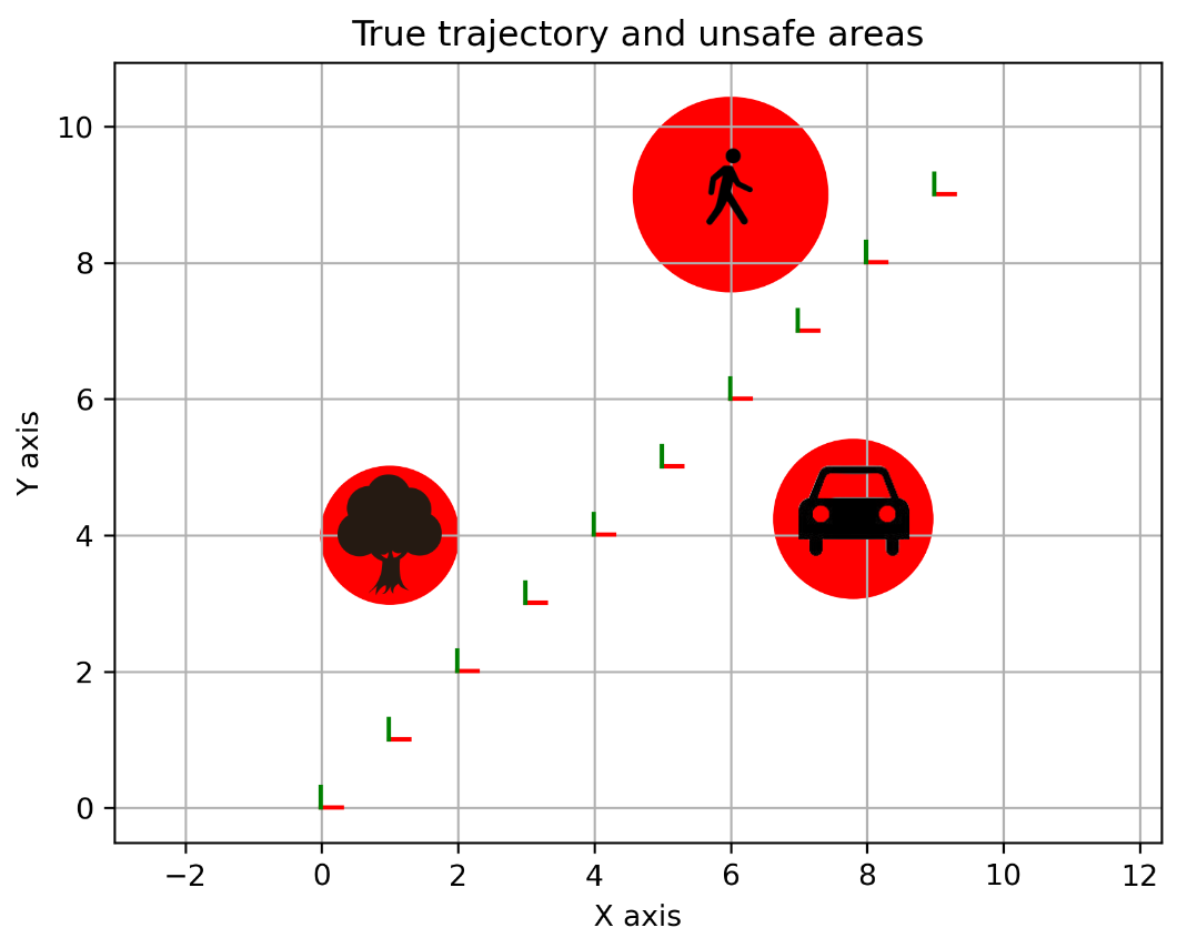
(a)

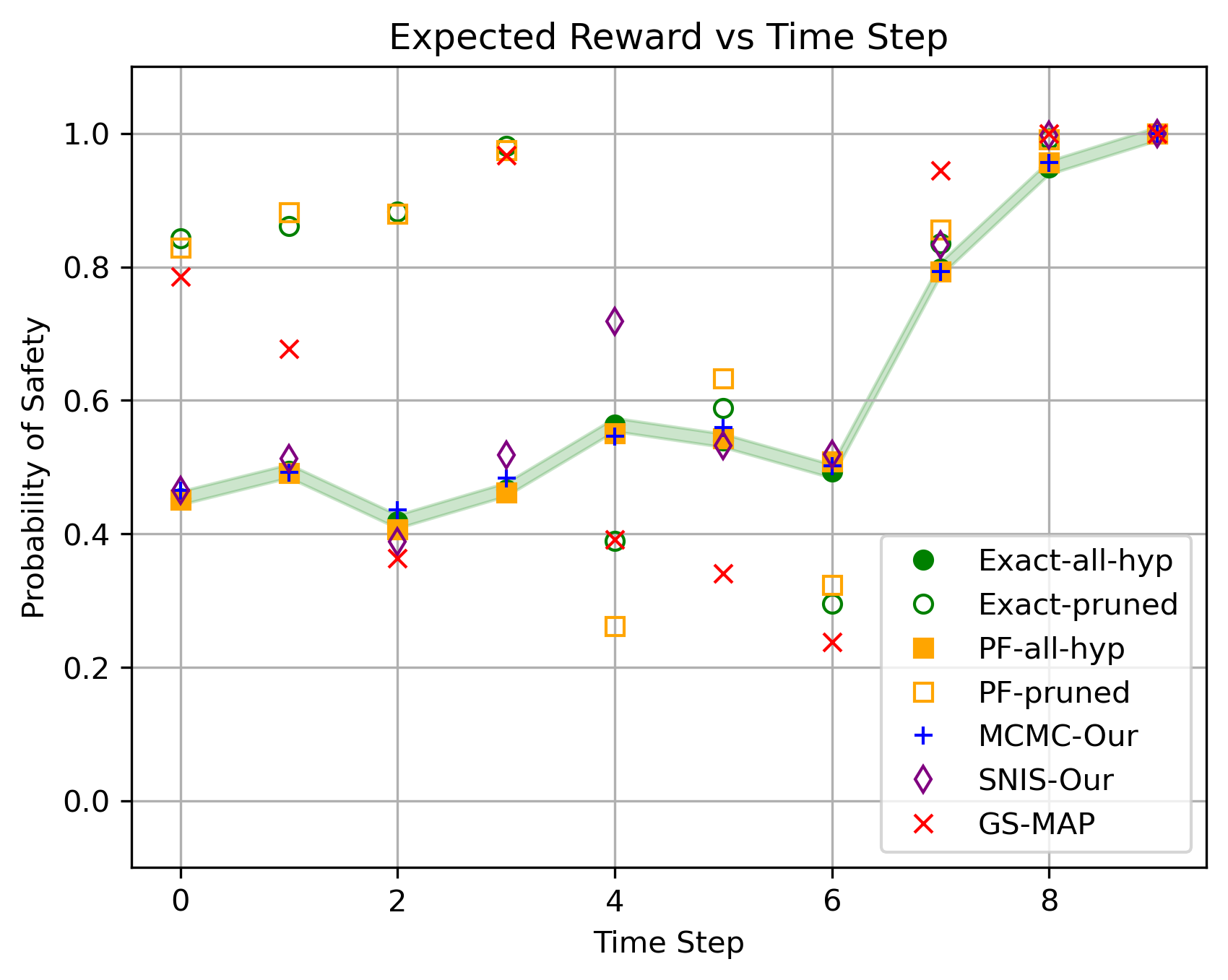
(b)

Figure 2: (a) The true trajectory and objects’ unsafe area. Robot starts at (0,0) and reaches (9,9). The class of an object specifies the unsafe area around it. Each time step, $\mathbb{P}_{\text{safe}}$ is calculated assuming the robot will continue to move in a straight line. (b) One trial probability of safety versus time, compared between different methods. In the case of the exact-all-hyp , Hoffding’s inequality holds, ensuring this result. For the rest of the estimators, MCMC-Ours and PF-all-hyp are aligned with the exact-all-hyp , SNIS-Ours is slightly further away, and exact-pruned , PF-pruned and GS-MAP are more biased. The bias can be positive or negative, and there is no indication as to which it will be. In the case of GS-MAP we get the least accurate results.

For the purpose of showing that the errors in the pruned estimators and in GS-MAP are caused by bias and not the sample size, we compared the root of the MSE (RMSE) versus the sample size in Figure 3. We used the same simulation as in Figure 2(b) previously. We calculated $\mathbb{P}_{\text{safe}}$ at time-step 4 for an increasing sample size for each estimator. This process was repeated 100 times and the result was averaged. According to our results, the error decreases with an increase in sample size for exact-all-hyp , PF-all-hyp , MCMC-Ours and SNIS-Ours . For the pruned methods and GS-MAP , the error does not decrease with sample size, indicating a bias.

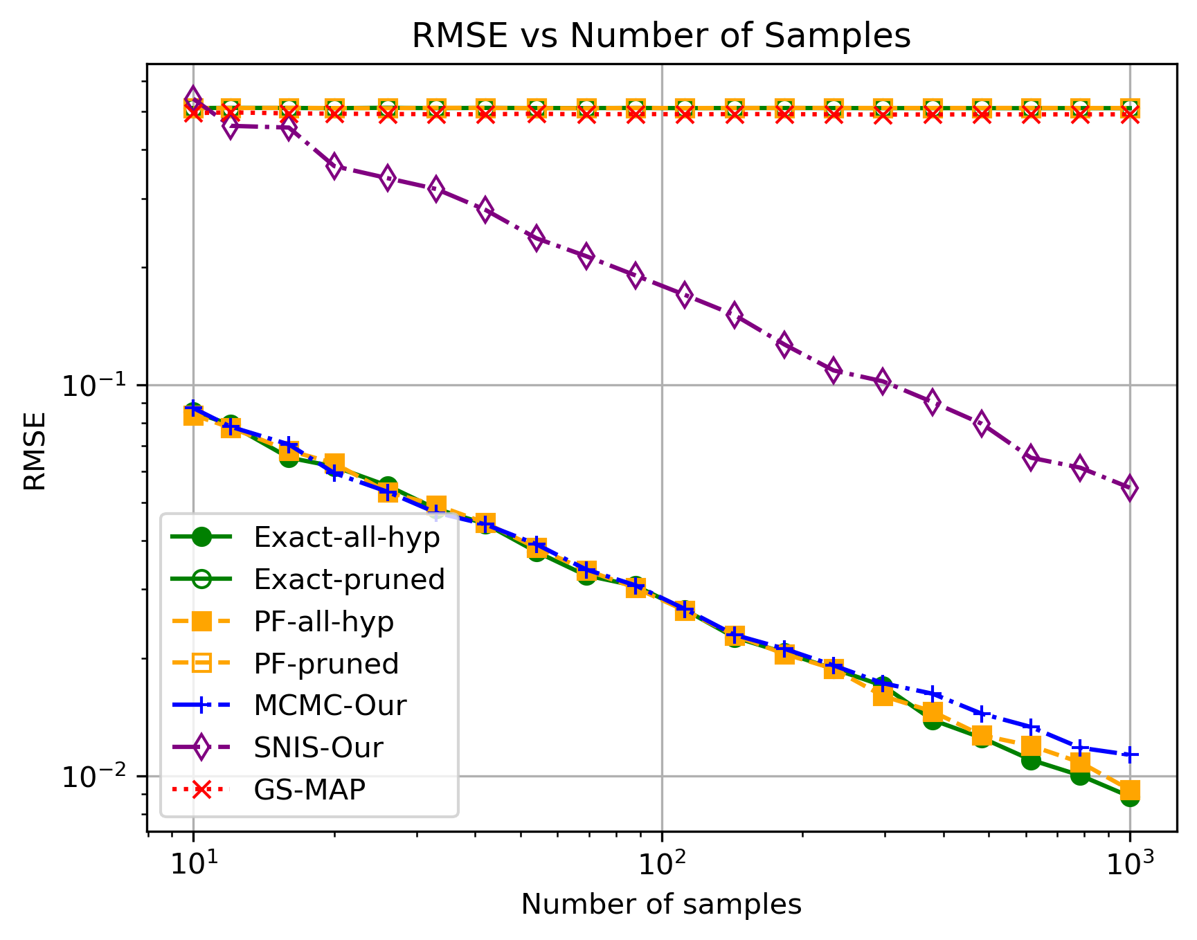
Figure 3: Expected reward error versus number of samples. The error decreases as the sample size increases for the exact-all-hyp , PF-all-hyp , MCMC-Ours and SNIS-Ours estimators. Exact-pruned , PF-pruned and GS-MAP estimators contain a bias that is not affected by sample size.

In the following simulation objects’ locations and classes were sampled randomly according to their prior probabilities. The robot’s true trajectory is sampled from the transition model. At each time step, the robot receives geometric and semantic observations. In this simulation, $\mathbb{P}_{\text{safe}}$ was estimated and the RMSE was evaluated, as depicted in Figure 4. This simulation was repeated for $10^{3}$ trials. All methods use $10^{3}$ samples. The true expected value is computed using the exact-all-hyp with $10^{6}$ samples. MCMC-Ours , PF-all-hyp and exact-all-hyp achieve similar results. The RMSE of SNIS-Ours is higher. However, the pruned versions and GS-MAP RMSEs are significantly higher.

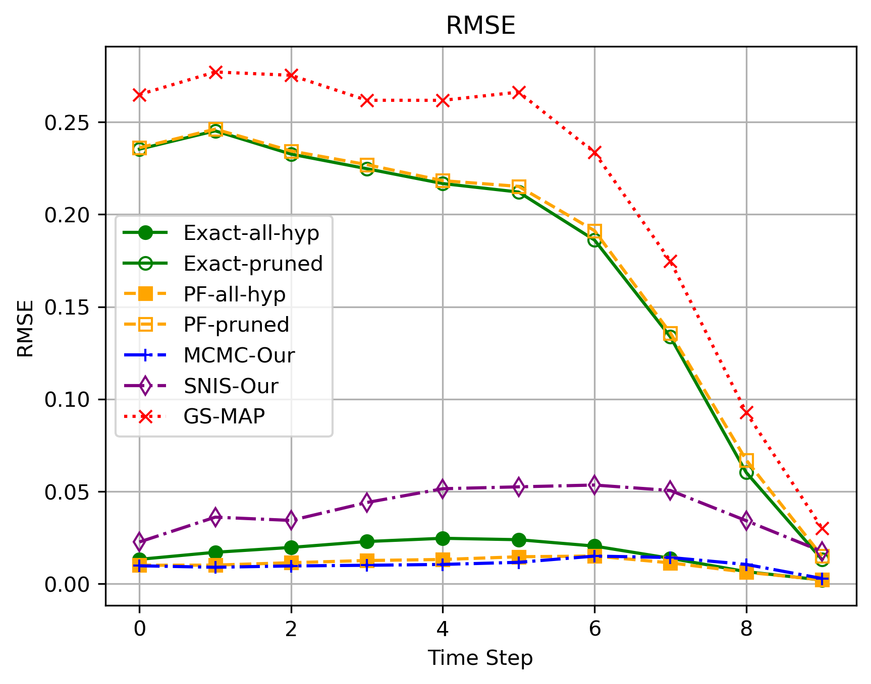
Figure 4: RMSE of $\mathbb{P}_{\text{safe}}$ estimations versus time-step.

In Figure 5, the RMSE and running time are presented against the number of classes. The simulation consisted of 600 trials. The environment consists of 3 objects randomly selected according to the prior probability at the beginning of each trial. An increase in the number of classes increases the state space size, but does not change the state dimensionality. Results in Figure 5(a) shows that the RMSEs of pruned estimates and GS-MAP estimate increase as the number of classes $N^{c}$ increases. Figure 5(b) shows linear complexity of MCMC-Ours , exponential complexity for exact-all-hyp and PF-all-hyp , and no noticeable increase in complexity for the pruned versions, GS-MAP, and SNIS-Ours .

(a)

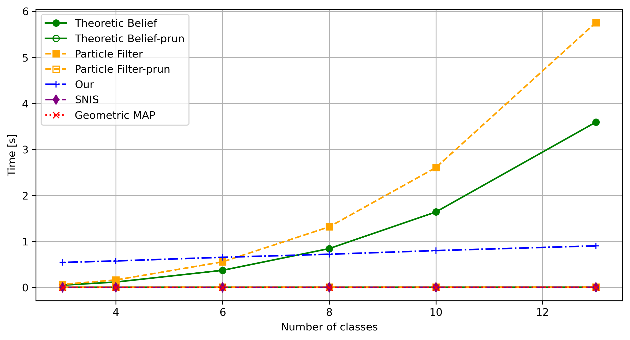
(b)

Figure 5: (a) RMSE $\mathbb{P}_{\text{safe}}$ estimations and (b) runtime versus number of classes. MCMC-Ours achieves the same accuracy as the exact-all-hyp and PF-all-hyp estimates, but with a linear instead of exponential runtime in the number of classes. SNIS-Ours has a slightly worse RMSE, but runs very efficiently. Exact-pruned , PF-pruned and GS-MAP are significantly less accurate.

As expected, the runtime of the exact-all-hyp and PF-all-hyp increases exponentially with the number of classes, the runtime of the pruned methods, SNIS-Ours and GS-MAP remains constant, and the runtime of MCMC-Ours increases linearly.

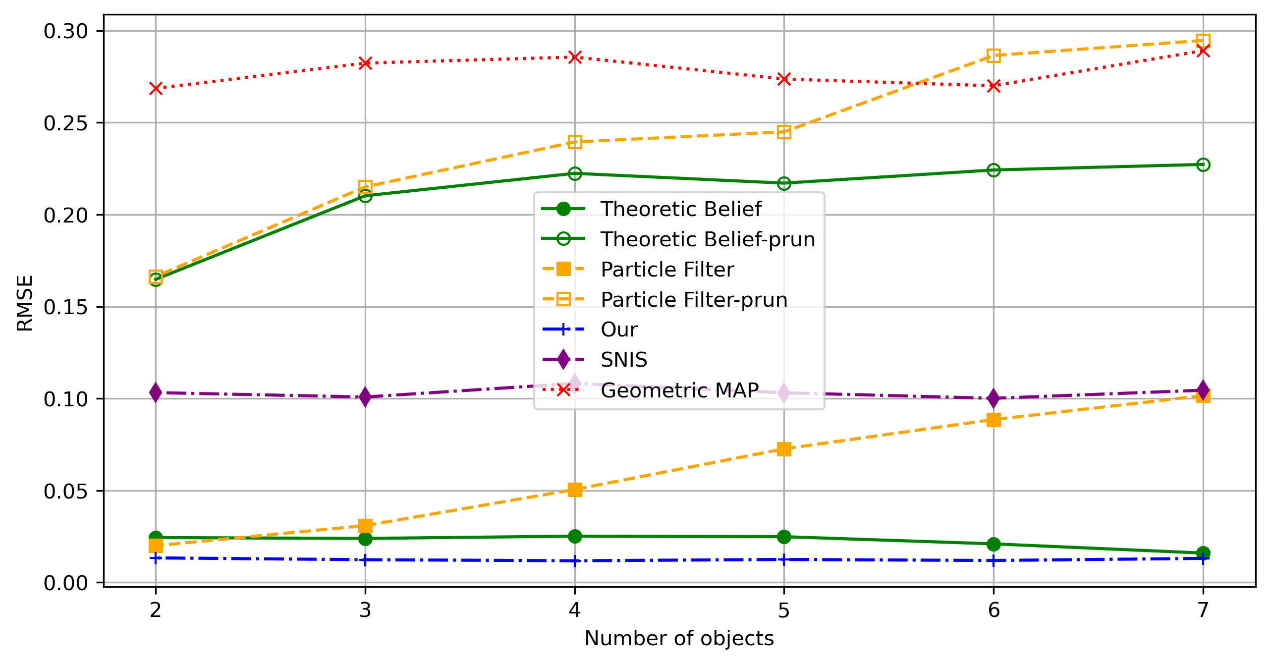
(a)

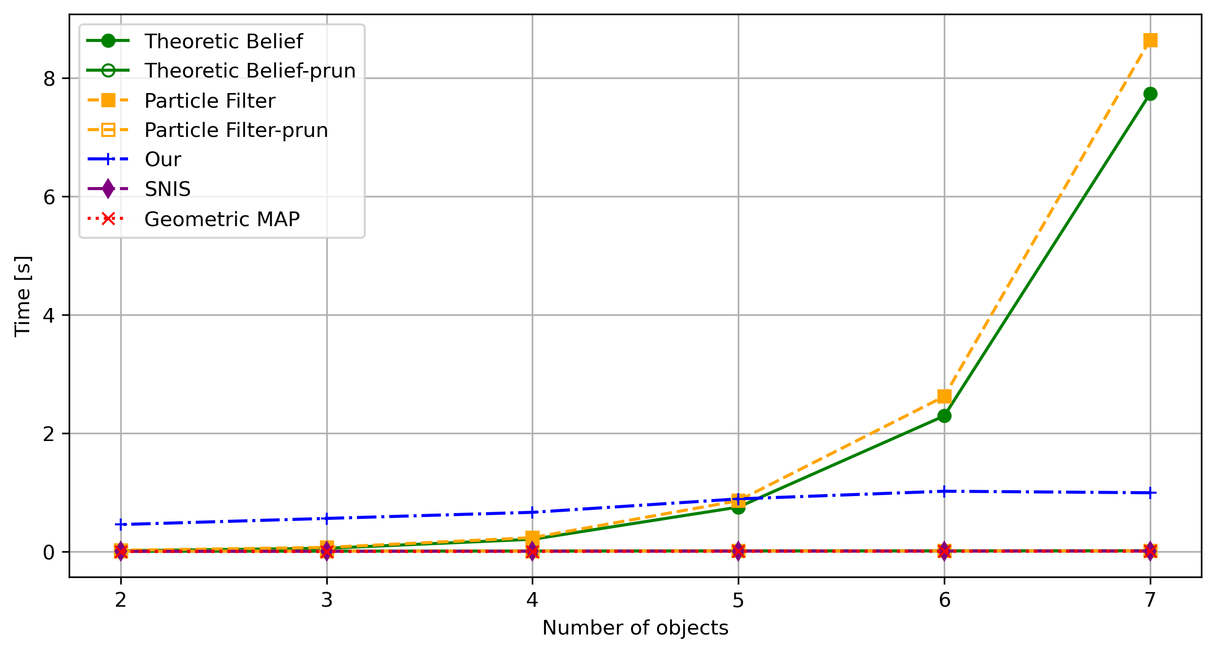
(b)

Figure 6: (a) RMSE of estimators of $\mathbb{P}_{\text{safe}}$ and (b) running time versus number of objects.

In Figure 6, the RMSE and running time are shown versus the number of objects. There are 600 trials conducted and the results are averaged. In all trials, the number of classes was 4. The environment consists of $N^{o}$ randomly selected objects at the beginning of each trial. An increase in the number of objects increases the dimensionality of the state. This affects the accuracy of the particle filter method. This is a well-known phenomenon in particle filtering known as the curse of dimensionality. Figure 6(a) shows an increase in RMSE as the number of objects increases for PF-all-hyp . Consequently, the RMSE of PF-pruned estimator also increases. In contrast, the error in exact-all-hyp , MCMC-Ours , and SNIS-Ours does not increase. As the number of objects increases, both MCMC-Ours and exact-all-hyp estimators maintain a very similar RMSEs.

Figure 6(b) shows that the runtime of exact-all-hyp and PF-all-hyp estimators increase exponentially with the number of objects. In contrast, the runtime of pruned version, SNIS-Ours and GS-MAP remains constant. MCMC-Ours runtime increases linearly. This is consistent with the theoretical runtime of the estimators in Table I.

VI-C Planning using the belief and safety constraint

Here, we demonstrate the effect of different estimators on the safety constraint and the robot’s actions. In this simulation, the robot decides what actions to take and executes them. The first four actions are the same for all methods and are predefined. Next, at each time-step the robot receives $N$ shortest paths from a probabilistic roadmap (PRM) and chooses the action that minimizes expected cost function under the constraint $\mathbb{P}_{\text{safe}}\geq 0.95$. The cost function is defined as $r_{t}(X_{t},a_{t})=||x_{t}-x_{g}||+||a_{t}||$ where $x_{g}=(10,10)$ is the goal points. Each method estimates these terms differently, and therefore chooses a different path. Figure 7(a) illustrates the true unsafe areas of the objects (in red) that correspond to the unknown true classes of the objects, as well as the four predefined actions and the $N$ shortest paths from the PRM.

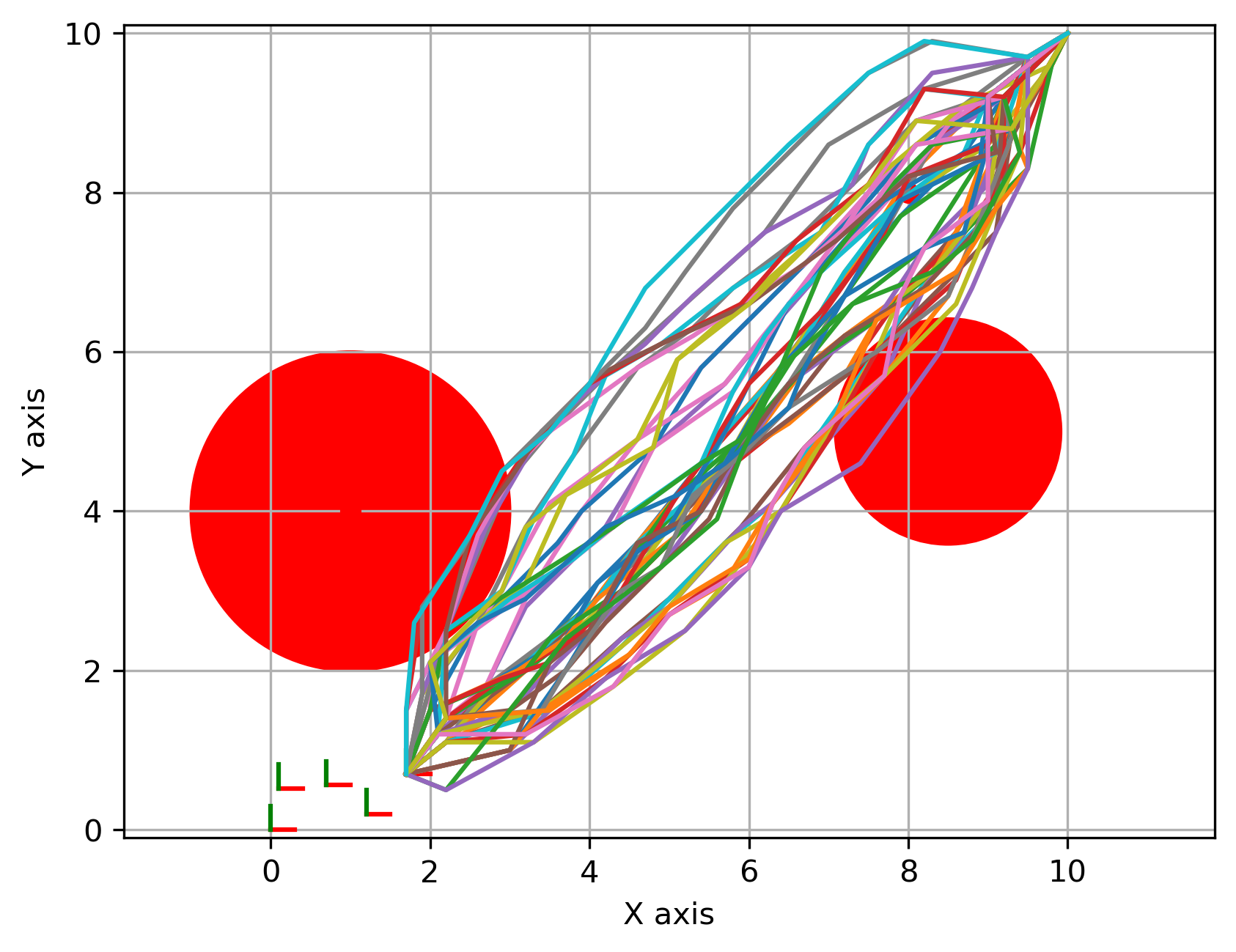
(a)

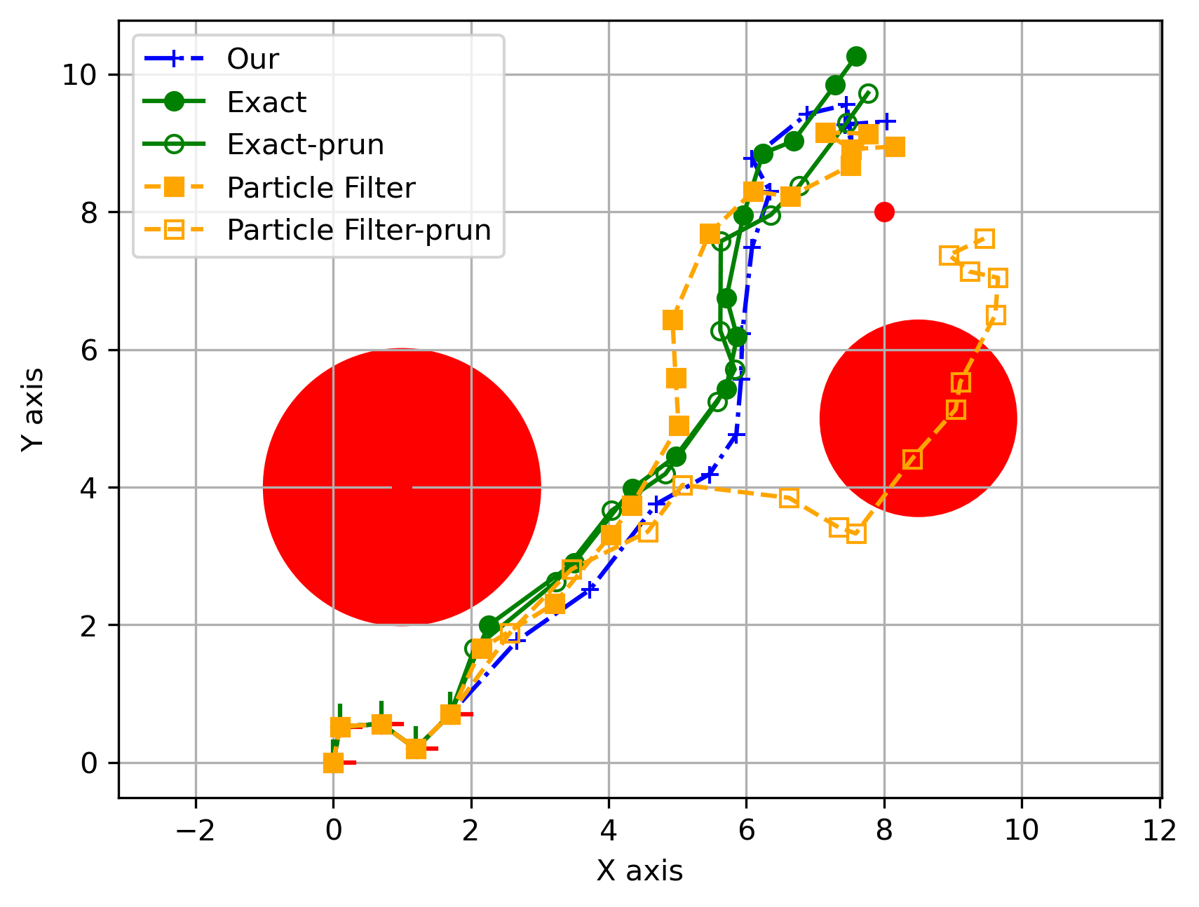
(b)

Figure 7: (a) Scene: four predefined actions, objects’ true unsafe areas, and $N$ shortest paths to goal from the PRM. (b) Chosen trajectory by each of the methods.

Upon receiving geometric and semantic observations and $N$ shortest paths, the robot calculates the probability of safety and expected reward for each path. The path that maximizes the expected reward and meets the safety constraints is selected. In the absence of a safe path the robot stops. In Figure 7(b), we show one trial of the simulation.

In Table II the results of $100$ trials are summarized. The results show that MCMC-Ours and exact-all-hyp are the most accurate in evaluating $\mathbb{P}_{\text{safe}}$ and the objective function, as they both achieved the highest success rate in finding a safe trajectory and minimizing the expected cost. The running time of this simulation is consistent with those of previous simulations, Figures 6(b) and 5(b).

Belief representation	Safe trajectory	Mean distance to goal if safe $\pm$ std	Mean trajectory length $\pm$ std
Exact-all-hyp	96/100	3.74 $\pm$ 2.21	14.75 $\pm$ 2.46
Exact-pruned	91/100	3.76 $\pm$ 2.52	14.60 $\pm$ 2.59
PF-all-hyp	87/100	10.28 $\pm$ 4.54	9.27 $\pm$ 4.39
PF-pruned	81/100	8.65 $\pm$ 4.62	10.56 $\pm$ 4.36
MCMC-Ours	96/100	3.73 $\pm$ 2.31	15.11 $\pm$ 2.63
SNIS-Ours	94/100	6.28 $\pm$ 3.02	13.05 $\pm$ 3.75

TABLE II: Trials of executing optimal action under the safety constraint that $\mathbb{P}_{\text{safe}}\geq 0.95$.

VII Conclusions

We present a novel approach for estimating the value function and objective function in a hybrid semantic-geometric POMDP, where observation models and prior probabilities are assumed to couple the geometric and semantic variables. The coupling between the variables causes all semantic variables to be dependent, leading to a combinatorial number of semantic hypotheses. We introduce the notion of semantically aware safety within POMDP, in which the robot is required to fulfill constraints that depend on semantic and geometric properties. In the described setting, it is very challenging to obtain representative samples of the belief required for estimating the value function and the safety probability. Under some assumptions, the MSE of the sample-based estimator will be exponential asymptotically. As a key contribution, we develop a novel factorization of the hybrid belief and leverage it to provide two methods for obtaining representative samples that do not result in an exponential MSE. The methods are 1) Approximating samples to theoretical beliefs using MCMC. 2) Utilizing importance sampling with a special proposal distribution form. As another key contribution, we show that under some assumptions and certain structured rewards, the expected reward can be computed efficiently with an explicit expectation over all possible semantic mappings, further reducing estimation error. We prove that the probability of safety falls under this structured reward. Our empirical simulations show that our approaches achieve similar accuracy as explicitly going through all the semantic hypotheses, but in a linear complexity rather than exponential. We believe this work paves the way for more reliable and safer autonomous robots that operate in complex semantic-geometric environments.

Appendix A Appendix

In the appendix we denote future observations $z_{k+1:t}$ as $z_{k}^{+}$, future policies $\pi_{k+1:T}$ as $\pi_{k}^{+}$, and future actions $a_{k:t-1}$ as $a_{k}^{+}$.

A-A Proof of Lemma III.1

Proof.

The value function (8) is the sum of expected rewards. We can examine a single expected reward since expectation is a linear operation. A single expected reward at a future time $t$ is given by

$$\underset{z_{k:t}}{\mathbb{E}}\left[\rho_{t}\right]=\underset{z_{k:t}}{\mathbb{E}}\left[\underset{b_{t}\left[C,X_{t}\right]}{\mathbb{E}}\left[r_{t}\right]\right]=\\ \intop_{z_{k:t}}\mathbb{P}\left(z_{k:t}\mid H_{k},\pi_{k:t}\right)\sum_{C}\intop_{X_{t}}\mathbb{P}\left(C,X_{t}\mid H_{t}\right)r_{t}.$$ (45)

Using Bayes’ theorem and chain rule, we can extract the last observation $z_{t}$ from $\mathbb{P}\left(C,X_{t}\mid H_{t}\right)$ and $\mathbb{P}\left(z_{k:t}\mid H_{k},\pi_{k:t}\right)$, respectively. Thus

$$\underset{z_{k:t}}{\mathbb{E}}\left[\rho_{t}\right]=\intop_{z_{k:t}}\cancel{\mathbb{P}\left(z_{t}\mid H_{t-1},a_{t-1}\right)}\mathbb{P}\left(z_{k:t-1}\mid H_{k},\pi_{k:t-1}\right)\times\\ \sum_{C}\intop_{X_{t}}\frac{\mathbb{P}_{Z}\left(z_{t}\mid C,X_{t}\right)\mathbb{P}_{T}\left(x_{t}\mid a_{t-1},x_{t-1}\right)\mathbb{P}\left(C,X_{t-1}\mid H_{t-1}\right)}{\cancel{\mathbb{P}\left(z_{t}\mid H_{t-1},a_{t-1}\right)}}r_{t}=\\ \intop_{z_{k:t-1}}\mathbb{P}\left(z_{k:t-1}\mid H_{k},\pi_{k:t-1}\right)\sum_{C}\intop_{X_{t}}\mathbb{P}\left(C,X_{t-1}\mid H_{t-1}\right)\times\\ \intop_{x_{t}}\mathbb{P}_{T}\left(x_{t}\mid a_{t-1},x_{t-1}\right)\intop_{z_{t}}\mathbb{P}_{Z}\left(z_{t}\mid C,X_{t}\right)r_{t},$$ (46)

where $a_{t-1}$ is well defined since $a_{t-1}=\pi_{t-1}\left(b_{t-1}\right)$ and $b_{t-1}$ obtained given $H_{t-1}$. Recursively repeat step (46) until time-step $k$, we obtain

$$\underset{z_{k:t}}{\mathbb{E}}\left[\rho_{t}\right]=\sum_{C}\intop_{X_{k}}\mathbb{P}\left(C,X_{k}\mid H_{k}\right)\times\\ \intop_{x_{k+1}}\mathbb{P}_{T}\left(x_{k+1}\mid a_{k},x_{k}\right)\intop_{z_{t}}\mathbb{P}_{Z}\left(z_{k+1}\mid C,X_{k+1}\right)\cdots\\ \intop_{x_{t}}\mathbb{P}_{T}\left(x_{t}\mid a_{t-1},x_{t-1}\right)\intop_{z_{t}}\mathbb{P}_{Z}\left(z_{t}\mid C,X_{t}\right)r_{t}$$ (47)

Finally, using expectation notation and considering the value function is the sum of the expected rewards, the value function is obtained by

$$V_{k}\left(b_{k},\pi_{k:L}\right)=\\ \underset{b_{k}\left[C,X_{k}\right]}{\mathbb{E}}\prod_{\tau=k+1}^{t}\underset{\mathbb{P}_{T}\left(x_{\tau}\mid\pi_{\tau-1},x_{\tau-1}\right)}{\mathbb{E}}\underset{\mathbb{P}_{Z}\left(z_{\tau}\mid X^{o},x_{\tau},C\right)}{\mathbb{E}}\left[\sum_{t=k}^{t}r_{t}\right].$$ (48)

Assuming a state dependent reward $r_{t}=r_{t}\left(X_{t},C,a_{t}\right)$ and open loop settings. Then, future observations do not participate in calculating the expectation in (48). Therefore, future observations are marginalized, and the objective function is given by

$$J\left(b_{k},a_{k:L}\right)=\\ \underset{b_{k}\left[C,X_{k}\right]}{\mathbb{E}}\prod_{\tau=k+1}^{t}\underset{\mathbb{P}_{T}\left(x_{\tau}\mid a_{\tau-1},x_{\tau-1}\right)}{\mathbb{E}}\left[\sum_{t=k}^{t}r\left(C,X_{t},a_{t}\right)\right].$$ (49)

∎

A-B Proof of Lemma V.1

Proof.

Previously in [26], we showed that the belief can be formulated as follows

$$b_{k}\left[X_{k},C\right]=\\ \frac{\tilde{\eta}_{1:k}}{\eta_{1:k}^{g}}b_{k}^{g}\left[X_{k}\right]\prod_{n=1}^{N^{o}}\tilde{b}_{k}\left[c_{n}\mid X_{k}\right],$$ (50)

where $\eta_{1:k}^{g}$ is the normalization factor of the geometric belief (22). The following terms are defined for clarity. $\eta_{1:k}\triangleq\frac{\tilde{\eta}_{1:k}}{\eta_{1:k}^{g}}$, is the normalization factor of (50), $\varphi_{n}\left(x_{1:k},x^{o}_{n}\right)\triangleq\sum_{c_{n}=1}^{N^{c}}\tilde{b}_{k}\left[c_{n}\mid X_{k}\right]$ is the normalizer of $\tilde{b}_{k}\left[c_{n}\mid X_{k}\right]$, $b_{k}\left[c_{n}\mid X_{k}\right]=\frac{\tilde{b}_{k}\left[c_{n}\mid X_{k}\right]}{\varphi_{n}\left(x_{1:k},x^{o}_{n}\right)}$, is the normalized semantic conditional belief of the $n$th object, and $\Phi\left(X_{k}\right)\triangleq\prod_{n=1}^{N^{o}}\varphi_{n}\left(x_{1:k},x^{o}_{n}\right)$ is the total semantic contribution to the belief. Accordingly, we can rewrite the belief as follows

$$b_{k}\left[C,X_{k}\right]=\eta_{1:k}b^{g}_{k}\left[X_{k}\right]\Phi\left(X_{k}\right)\prod_{n=1}^{N^{o}}b_{k}\left[c_{n}\mid X_{k}\right].$$ (51)

Since the only term in (51) that is dependent on the class of the $n$th object is $b_{k}\left[c_{n}\mid X_{k}\right]$, the marginal beliefs $b_{k}\left[c_{n}\right]$ and $b_{k}\left[X_{k}\right]$ are given by

$$b_{k}\left[X_{k}\right]=\eta_{1:k}b^{g}_{k}\left[X_{k}\right]\Phi\left(X_{k}\right),$$ (52)

$$b_{k}\left[c_{n}\right]=\intop_{X_{k}}b_{k}\left[X_{k}\right]b_{k}\left[c_{n}\mid X_{k}\right]dX_{k}.$$ (53)

∎

A-C Proof of Theorem V.5

To prove Theorem V.5, we first have to prove that the posterior probability $\mathbb{P}(C\mid H_{k})$ is asymptotically concentrated on the true hypothesis. This is done in Proposition A.1. We use explicit notation of the posterior probability $\mathbb{P}(C\mid H_{k})$ instead of $b_{k}\left[C\right]$, since we are looking at the asymptotic behavior and considering different realizations of the true hypothesis $C^{tr}$ and history $H_{k}$.

Proposition A.1.

The posterior $\mathbb{P}(C\mid H_{k})$ asymptotically converges to $1$ at $C^{tr}$.

Proof.

Since MAP is consistent, for any $\epsilon>0$, there exists a time index $K$ such that for any $k>K$, then

$$\mathbb{P}\left(C_{MAP}^{k}=C^{tr}\right)\geq 1-\epsilon.$$ (54)

In order to fulfill (54) it requires that also $\mathbb{P}(C^{tr}\mid H_{k})\geq 1-\epsilon$ to hold. ∎

It should be noted that the posterior $\mathbb{P}(C\mid H_{k})$ is dependent on $C^{tr}$ through the observations in $H_{k}$.

We now proceed to the proof of Theorem V.5.

Proof.

Consider obtaining a realization of $C^{tr}$ and $H_{k}$, and consider using $N^{s}$ samples. Then, $\hat{\mathbb{E}}_{IS}^{\left(X,C\right)}$ is given by

$$\hat{\mathbb{E}}_{IS}^{\left(X,C\right)}\triangleq\frac{1}{N^{s}}\frac{\mathbb{P}(X_{k}^{(i)},C^{(i)}\mid H_{k})}{q\left(X_{k}^{(i)},C^{(i)}\right)}g\left(X_{k}^{(i)},C^{(i)}\right).$$ (55)

According to Theorem V.6, by calculating the explicit expectation over $X_{k}$ and taking only samples of $C$, estimation MSE will be reduced

$$\text{MSE}\left(\hat{\mathbb{E}}^{IS\left(X,C\right)}\right)\geq\text{MSE}\left(\hat{\mathbb{E}}^{IS(C)}\right).$$ (56)

Define $\bar{g}\left[C\right]=\underset{X_{k}\mid C}{\mathbb{E}}\left[g\left(X_{k},C\right)\mid C\right]$, thus $\hat{\mathbb{E}}^{IS(C)}\triangleq\frac{1}{N^{s}}\frac{\mathbb{P}(C^{(i)}\mid H_{k})}{q\left(C^{(i)}\right)}\bar{g}(C^{(i)}).$ According to [47] the MSE of $\hat{\mathbb{E}}^{IS(C)}$ is obtained by

$$\text{MSE}\left(\hat{\mathbb{E}}^{IS(C)}\mid C^{tr},H_{k}\right)=\\ \frac{\mathbb{E}_{q}\left[\left(\frac{\mathbb{P}(C\mid H_{k})}{q(C)}\right)^{2}g^{2}(C)\right]}{N^{s}}-\mu_{g}^{2}=\sum_{C\in\mathcal{C}}\frac{\mathbb{P}^{2}(C\mid H_{k})}{N^{s}q(C)}\bar{g}^{2}(C)$$

where $\mu_{g}$ is the expected value of $g\left(X_{k},C\right)$. Marginalizing over $H_{k}$ and $C^{tr}$, the MSE obtained by

$$\text{MSE}\left(\hat{\mathbb{E}}^{IS}\right)=\\ \underset{\mathbb{P}_{0}(C^{tr})}{\mathbb{E}}\underset{H_{k}\mid C^{tr}}{\mathbb{E}}\left[\sum_{C\in\mathcal{C}}\frac{\mathbb{P}^{2}(C\mid H_{k})}{N^{s}q(C)}g^{2}(C)\right]-\mu_{g}^{2}.$$ (57)

Moving $N^{s}$ and $\mu_{g}$ to the MSE side of (57) and using Proposition (A.1) one obtains

$$L_{1}\triangleq\left(\text{MSE}\left(\hat{\mathbb{E}}^{IS}\left[\bar{g}\right]\right)+\mu_{g}^{2}\right)N^{s}\geq\\ \underset{\mathbb{P}_{0}(C^{tr})}{\mathbb{E}}\underset{H_{k}\mid C^{tr}}{\mathbb{E}}\left[\left(\frac{(1-\epsilon)^{2}}{q(C^{tr})}+\sum_{C\in\mathcal{C}\lnot C^{tr}}\frac{\epsilon^{2}}{q(C)}\bar{g}^{2}(C)\right)\right]\triangleq L_{2}.$$ (58)

Since $L_{2}$’s integrand does not include $H_{k}$, and $q(C)$ is assumed to be independent of $H_{k}$ (Assumption V.4), (Assumption 2), $H_{k}$ can be marginalized from (58)

$$L_{2}=\underset{\mathbb{P}_{0}(C^{tr})}{\mathbb{E}}\left[\left(\frac{(1-\epsilon)^{2}}{q(C^{tr})}+\sum_{C\in\mathcal{C}\lnot C^{tr}}\frac{\epsilon^{2}}{q(C)}\bar{g}^{2}(C)\right)\right]=\\ \\ =(1-\epsilon)^{2}\sum_{C^{tr}}\frac{\mathbb{P}_{0}(C^{tr})}{q(C^{tr})}\bar{g}^{2}(C^{tr})+\epsilon^{2}\sum_{C\in\mathcal{C}\lnot C^{tr}}\frac{\bar{g}^{2}(C)}{q(C)}\\ \geq(1-\epsilon)^{2}\sum_{C^{tr}}\frac{\mathbb{P}_{0}(C^{tr})}{q(C^{tr})}\bar{g}^{2}(C^{tr}).$$ (59)

Define $\tilde{w}(C)=\frac{\mathbb{P}_{0}(C^{tr})}{q(C^{tr})},\;\;\eta_{w}^{-1}=\sum_{C\in\mathcal{C}}w(C)$, and $w(C)=\eta_{w}\tilde{w}(C)$. $w(C)$ can be interpreted as a probability function. Returning $\mu_{g}$ and $N^{s}$ to the right side of (59) the lower bound of the MSE, denoted by $\underline{MSE}$, is obtained by

$$\underline{MSE} =\frac{1}{N^{s}}(1-\epsilon)^{2}\eta_{w}^{-1}\sum_{C^{tr}}w(C)g^{2}(C^{tr})-\mu_{g}^{2}$$

$$=\frac{1}{N^{s}}(1-\epsilon)^{2}\eta_{w}^{-1}\underset{w}{\text{Var}}\left[\bar{g}\right]$$

$$\approx\frac{1}{N^{s}}\eta_{w}^{-1}\underset{w}{\text{Var}}\left[\bar{g}\right].$$

$\eta_{w}^{-1}$ is minimized when $q(C)=\mathbb{P}_{0}(C)\;\;\forall C\in\mathcal{C}$. This can be proven using Lagrange multipliers. Therefore, the bound is obtained by

$$\text{MSE}\left(\hat{\mathbb{E}}^{IS(C)}\right)\geq\frac{1}{N^{s}}\left|\mathcal{C}\right|\underset{w}{\text{Var}}\left[\bar{g}\right].$$ (60)

Finally, according to (56), we get

$$\text{MSE}\left(\hat{\mathbb{E}}^{IS\left(X,C\right)}\right)\geq\frac{1}{N^{s}}\left|\mathcal{C}\right|\underset{w}{\text{Var}}\left[\bar{g}\right].$$ (61)

∎

A-D Proof of Theorem V.6

Proof.

Consider approximating the expectation $\underset{X,Y}{\mathbb{E}}\left[g\left(X,C\right)\right]$ using iid samples $X^{(i)},C^{(i)}\sim\mathbb{P}\left[X,C\right],\>\>i=1,\cdots,N^{s}$, thus $\hat{\mathbb{E}}^{(X,C)}\triangleq\frac{1}{N^{s}}\sum_{i=1}^{N^{s}}g\left(X^{(i)},C^{(i)}\right).$ This is an unbiased estimation with variance $\text{Var}\left(\hat{\mathbb{E}}^{(X,C)}\right)=\frac{1}{N^{s}}\text{Var}\left(g\left(X,C\right)\right).$ Consider another estimator by taking samples of $X$ and explicitly calculating the conditional expectation over $C$, thus $\hat{\mathbb{E}}^{(X)}=\frac{1}{N^{s}}\sum_{i=1}^{N^{s}}\underset{C\mid X}{\mathbb{E}}\left[g\left(X^{(i)},C\right)\mid X=X^{(i)}\right].$ This is also an unbiased estimator with the variance $\text{Var}\left(\hat{\mathbb{E}}^{(X)}\right)=\frac{1}{N^{s}}\text{Var}\left(\underset{C\mid X}{\mathbb{E}}\left[g\left(X,C\right)\mid X\right]\right)$. The difference between the variances is

$$\text{Var}\left(\hat{\mathbb{E}}^{(X,C)}\right)-\text{Var}\left(\hat{\mathbb{E}}^{(X)}\right)=\\ =\frac{1}{N^{s}}\underset{X,C}{\mathbb{E}}\left[g^{2}\left(X,C\right)\right]-\frac{1}{N^{s}}\underset{X}{\mathbb{E}}\left[\underset{C\mid X}{\mathbb{E}}^{2}\left[g\left(X,C\right)\mid X\right]\right]\\ =\frac{1}{N^{s}}\left(\underset{X}{\mathbb{E}}\left[\underset{C\mid X}{\mathbb{E}}\left[g^{2}\left(X,C\right)-\underset{C\mid X}{\mathbb{E}}^{2}\left[g\left(X,C\right)\right]\mid X\right]\right]\right)\\ =\frac{1}{N^{s}}\underset{X}{\mathbb{E}}\left[\underset{C\sim\mathbb{P}\left(C\mid X\right)}{\text{Var}}\left(g\left(X,C\right)\right)\right],$$ (62)

where the last line is holds by using the identity $\text{Var}\left(\psi\right)=\mathbb{E}\left[\psi^{2}\right]-\mathbb{E}^{2}\left[\psi\right]$ inside the expectation on $X$. Since the variance of an unbiased estimator is the MSE, the theorem is proven. ∎

A-E Proof of Lemma V.7

Proof.

Consider a single expected reward component $\underset{z_{k}^{+}}{\mathbb{E}}\left[\rho_{t}\left(b_{t},a_{t}\right)\right]$ of the value function (8). Formulating the expected reward explicitly and using Bayes’ theorem, it can be derived as follows

$$\underset{z_{k}^{+}}{\mathbb{E}}\left[\rho_{t}\left(b_{t},a_{t}\right)\right]=\intop_{z_{k}^{+}}\mathbb{P}\left(z_{k}^{+}\mid H_{k},\pi_{k}^{+}\right)\intop_{X_{t}}\sum_{C}\mathbb{P}\left(X_{t},C\mid H_{t}\right)r_{t}=\\ \intop_{z_{k}^{+}}\mathbb{P}\left(z_{k}^{+}\mid H_{k},\pi_{k}^{+}\right)\intop_{X_{t}}\sum_{C}\mathbb{P}\left(X_{t},C\mid H_{k},z_{k}^{+},\pi_{k}^{+}\right)r_{t}=\\ \intop_{z_{k}^{+}}\cancel{\mathbb{P}\left(z_{k}^{+}\mid H_{k},\pi_{k}^{+}\right)}\intop_{X_{t}}\sum_{C}\frac{\mathbb{P}\left(z_{k}^{+}\mid X_{t},C\right)\mathbb{P}\left(X_{t},C\mid H_{k},\pi_{k}^{+}\right)}{\cancel{\mathbb{P}\left(z_{k}^{+}\mid H_{k},\pi_{k}^{+}\right)}}r_{t}=\\ \intop_{z_{k}^{+}}\intop_{X_{t}}\sum_{C}\mathbb{P}\left(z_{k}^{+}\mid X_{t},C\right)\mathbb{P}\left(X_{t},C\mid H_{k},\pi_{k}^{+}\right)r_{t},$$ (63)

where the future beliefs $b_{t}\left[X_{t},C\right]$ and actions $a_{t}$ are defined uniquely by $H_{k}$, the future observations $z_{k}^{+}$, and the policies $\pi_{k}^{+}$. The future beliefs and action can be calculated as by defining the update operator $b_{\tau+1}\triangleq\varphi(b_{\tau},a_{\tau},z_{\tau+1})$. The they are obtained recursively by $a_{\tau}=\pi_{\tau}\left(b_{\tau}\right)$ and $b_{\tau+1}=\varphi\left(b_{\tau},a_{\tau},z_{\tau+1}\right)$. Using chain rule we can refactor the follows probability

$$\mathbb{P}\left(X_{t},C\mid H_{k},\pi_{k}^{+}\right)=\mathbb{P}\left(X_{t}\mid H_{k},\pi_{k}^{+}\right)\mathbb{P}\left(C\mid X_{t},H_{k},\pi_{k}^{+}\right)$$ (64)

The semantic hypothesis $C$ is dependent on $X_{t}$ only through the prior probability and the observations that connect between them, therefore,

$$\mathbb{P}\left(C\mid X_{t},H_{k},\pi_{k}^{+}\right)=\mathbb{P}\left(C\mid X_{k},H_{k}\right).$$ (65)

By substituting (65) into (63), we obtain

$$\underset{z_{k}^{+}}{\mathbb{E}}\left[\rho_{t}\left(b_{t}\right)\right]=\\ \intop_{z_{k}^{+}}\intop_{X_{t}}\sum_{C}\mathbb{P}\left(z_{k}^{+}\mid X_{t},C\right)\mathbb{P}\left(X_{t}\mid H_{k},\pi_{k}^{+}\right)\mathbb{P}\left(C\mid X_{k},H_{k}\right)r_{t}.$$ (66)

This can be reformulated as follows

$$\underset{z_{k}^{+}}{\mathbb{E}}\left[\rho_{t}\left(b_{t},a_{t}\right)\right]=\underset{\mathbb{P}\left(X_{t}\mid H_{k},\pi_{k}^{+}\right)}{\mathbb{E}}\left[\underset{b_{k}\left[C\mid X_{k}\right]}{\mathbb{E}}\prod_{\tau=k+1}^{t}\underset{\mathbb{P}_{Z}\left(z_{\tau}\mid X_{\tau},C\right)}{\mathbb{E}}\left[r_{t}(\cdot)\right]\right].$$ (67)

Using the assumption that $r_{t}$ is state dependent, and it is not dependent on the action, or it is dependent on the action but the actions are predetermined in an open loop settings, then it is possible to marginalize the observations.

$$\underset{z_{k}^{+}}{\mathbb{E}}\left[\rho_{t}\left(b_{t},a_{t}\right)\right]=\underset{\mathbb{P}\left(X_{t}\mid H_{k},\pi_{k}^{+}\right)}{\mathbb{E}}\left[\underset{b_{k}\left[C\mid X_{k}\right]}{\mathbb{E}}\left[r_{t}(\cdot)\right]\right].$$ (68)

Finally, the value function is the sum of the expected rewards, therefore it can be written as follows

$$V_{k}\left(b_{k},\pi_{k:L}\right)=\underset{\mathbb{P}\left(X_{L}\mid H_{k},\pi_{k:L-1}\right)}{\mathbb{E}}\left[\underset{b_{k}\left[C\mid X_{k}\right]}{\mathbb{E}}\left[\sum_{t=k}^{L}r_{t}\left(\cdot\right)\right]\right].$$ (69)

∎

A-F Proof of Theorem V.8

Proof.

Consider the reward in (37). Define the following augmented element

$$\tilde{r}_{t,j,n}\left(c_{n},X_{t}\right)\triangleq\begin{cases}r_{t,j,n}\left(c_{n},X_{t}\right)&n\in\theta_{j}\\ 1&\text{otherwise}\end{cases}.$$ (70)

Using the augmented element (70), the reward (37) can be rewritten as follows

$$r_{t}\left(C,X_{t}\right)=\sum_{j=1}^{|\Theta|}\prod_{n=1}^{N^{o}}\tilde{r}_{t,j,n}\left(c_{n},X_{t}\right).$$ (71)

Since expectation is a linear operation, we can take the sum in (71) out of the expectation and return it latter. For now, consider that the reward above (71) consist of only one element of the sum,

$$r_{t}\left(C,X_{t}\right)=\prod_{n=1}^{N_{o}}\tilde{r}_{t,j,n}(c_{n},X_{t}).$$ (72)

Consider the expected reward (35) and using the above inner reward function (72), the expected reward can be formulated as follows

$$\underset{z_{k+1:t}}{\mathbb{E}}\left[\rho\left(b_{t}\right)\right]=\\ \underset{\mathbb{P}\left(X_{t}\mid H_{k},\pi_{k:t-1}\right)}{\mathbb{E}}\left[\underset{b_{k}\left[C\mid X_{k}\right]}{\mathbb{E}}\left[\prod_{n=1}^{N_{o}}\tilde{r}_{t,j,n}(c_{n},X_{t})\right]\right]=\\ \underset{\mathbb{P}\left(X_{t}\mid H_{k},\pi_{k:t-1}\right)}{\mathbb{E}}\sum_{C=1}^{N^{c}}\left[\prod_{n=1}^{N_{o}}b_{k}\left[c_{n}\mid X_{k}\right]\tilde{r}_{t,j,n}(c_{n},X_{t})\right].$$ (73)

To simplify notations we will use $\mathbb{P}^{+}(X_{t})=\mathbb{P}\left(X_{t}\mid H_{k},\pi_{k:t-1}\right)$. Since both $b_{k}\left[c_{n}\mid X_{k}\right]$ and $\tilde{r}_{t,j,n}(c_{n},X_{t})$ are dependent on the a single object class $c_{n}$, the expected reward (73) can be reorganized as follows

$$\underset{z_{k+1:t}}{\mathbb{E}}\left[\rho\left(b_{t}\right)\right]=\underset{\mathbb{P}^{+}(X_{t})}{\mathbb{E}}\left[\prod_{n=1}^{N^{o}}\sum_{c_{n}=1}^{N^{c}}b_{k}\left[c_{n}\mid X_{k}\right]\tilde{r}_{t,j,n}\left(c_{n},X_{t}\right)\right].$$ (74)

If $n\notin\theta_{j}$ the augmented element is equal to 1 and the sum in (74) result in $\sum_{c_{n}=1}^{N^{c}}b_{k}\left[c_{n}\mid X_{k}\right]\cdot 1$. Therefore we can simplify (74) to

$$\underset{z_{k+1:t}}{\mathbb{E}}\left[\rho\left(b_{t}\right)\right]=\underset{\mathbb{P}^{+}(X_{t})}{\mathbb{E}}\left[\prod_{n\in\theta_{j}}\underset{b_{k}\left[c_{n}\mid X_{k}\right]}{\mathbb{E}}\left[r_{t,j,n}\left(c_{n},X_{t}\right)\right]\right].$$ (75)

By restoring the full reward (37) into the expected reward (75), one obtains

$$\underset{z_{k+1:t}}{\mathbb{E}}\left[\rho\left(b_{t}\right)\right]=\underset{\mathbb{P}^{+}(X_{t})}{\mathbb{E}}\left[\sum_{j=1}^{|\Theta|}\prod_{n\in\theta_{j}}\underset{b_{k}\left[c_{n}\mid X_{k}\right]}{\mathbb{E}}\left[r_{t,j,n}\left(c_{n},X_{t}\right)\right]\right].$$ (76)

The approximation of the expected reward, we will use samples of $X_{t}^{(i)}\sim\mathbb{P}^{+}(X_{t})$ and approximate it as follows

$$\hat{\mathbb{E}}[\rho_{t}(b_{t})]=\\ \frac{1}{N^{s}}\sum_{i=1}^{N^{s}}\sum_{j=1}^{|\Theta|}\prod_{n\in\theta_{j}}\sum_{c_{n}=1}^{N^{c}}b_{k}\left[c_{n}\mid X_{k}^{(i)}\right]r_{t,j,n}\left(c_{n},X_{t}^{(i)}\right).$$ (77)

The computation complexity is $O\left(N^{s}N^{\Theta}N^{c}\right)$.

∎

A-G Proof of Proposition V.9

Proof.

Let $\rho$ be defined in (10). $\mathbb{P}_{\text{safe}}$ (13) can be formulated as an expectation over $X_{L},C\mid b_{k},\pi_{k:L-1}$ on the indicator function $\mathbf{1}\left[\wedge_{\tau=k+1}^{L}x_{\tau}\notin\mathcal{X}_{\text{unsafe}}\left(C,X^{o}\right)\right]$, thus

$$\mathbb{P}_{\text{safe}}=\mathbb{E}\left[\mathbf{1}\left[\wedge_{\tau=k+1}^{L}x_{\tau}\notin\mathcal{X}_{\text{unsafe}}\left(C,X^{o}\right)\right]\mid b_{k},\pi_{k:L}\right].$$ (78)

Marginalizing over future observations, we obtain

$$\mathbb{P}_{\text{safe}}=\\ \underset{z_{k:L}|b_{k},\pi_{k:L}}{\mathbb{E}}\left[\underset{X_{L},C|b_{L}}{\mathbb{E}}\left\{\mathbf{1}\left[\wedge_{\tau=k+1}^{L}x_{\tau}\notin\mathcal{X}_{\text{unsafe}}\left(C,X^{o}\right)\right]\right\}\right].$$ (79)

This is a state-dependent reward, with the indicator being the inner reward function $r_{safe}\left(X_{t},C\right)=\mathbf{1}\left[\wedge_{\tau=k+1}^{L}x_{\tau}\notin\mathcal{X}_{\text{unsafe}}\left(C,X^{o}\right)\right]$. Furthermore, $r_{safe}$ can be formulated as follows

$$r_{safe}\left(X_{t},C\right)=\mathbf{1}\left[\wedge_{\tau=k+1}^{L}x_{\tau}\notin\cup_{n=1}^{N^{o}}\mathcal{X}_{\text{unsafe}}\left(c_{n},x^{o}_{n}\right)\right]\\ =\prod_{n=1}^{N^{o}}\prod_{\tau=k+1}^{L}\mathbf{1}\left[x_{\tau}\notin\mathcal{X}_{\text{unsafe}}\left(c_{n},x^{o}_{n}\right)\right].$$ (80)

∎

References

- [1] J. Velez, G. Hemann, A. S. Huang, I. Posner, and N. Roy, “Modelling observation correlations for active exploration and robust object detection,” J. of Artificial Intelligence Research, 2012.
- [2] W. Chen, G. Shang, A. Ji, C. Zhou, X. Wang, C. Xu, Z. Li, and K. Hu, “An overview on visual slam: From tradition to semantic,” Remote Sensing, vol. 14, no. 13, p. 3010, 2022.
- [3] A. Nüchter and J. Hertzberg, “Towards semantic maps for mobile robots,” Robotics and Autonomous Systems, vol. 56, no. 11, pp. 915–926, 2008.
- [4] D. Kopitkov and V. Indelman, “Robot localization through information recovered from cnn classificators,” in IEEE/RSJ Intl. Conf. on Intelligent Robots and Systems (IROS). IEEE, October 2018.
- [5] Y. Feldman and V. Indelman, “Spatially-dependent bayesian semantic perception under model and localization uncertainty,” Autonomous Robots, 2020.
- [6] D. Morilla-Cabello, J. Westheider, M. Popović, and E. Montijano, “Perceptual factors for environmental modeling in robotic active perception,” in 2024 IEEE International Conference on Robotics and Automation (ICRA), 2024, pp. 4605–4611.
- [7] J. Crespo, J. C. Castillo, O. M. Mozos, and R. Barber, “Semantic information for robot navigation: A survey,” Applied Sciences, vol. 10, no. 2, p. 497, 2020.
- [8] R. D. Smallwood and E. J. Sondik, “The optimal control of partially observable markov processes over a finite horizon,” Operations Research, vol. 21, no. 5, pp. 1071–1088, 1973.
- [9] M. T. Spaan and N. Spaan, “A point-based pomdp algorithm for robot planning,” in IEEE International Conference on Robotics and Automation, 2004. Proceedings. ICRA’04. 2004, vol. 3. IEEE, 2004, pp. 2399–2404.
- [10] H. Kurniawati, “Partially observable markov decision processes and robotics,” Annual Review of Control, Robotics, and Autonomous Systems, vol. 5, no. 1, pp. 253–277, 2022.
- [11] H. Kurniawati, T. Bandyopadhyay, and N. M. Patrikalakis, “Global motion planning under uncertain motion, sensing, and environment map,” in Robotics: Science and Systems VII, University of Southern California, Los Angeles, CA, USA, June 27-30, 2011, 2011.
- [12] V. Tchuiev and V. Indelman, “Epistemic uncertainty aware semantic localization and mapping for inference and belief space planning,” Artificial Intelligence, p. 103903, 2023.
- [13] S. Yang and S. Scherer, “Cubeslam: Monocular 3-d object slam,” IEEE Transactions on Robotics, vol. 35, no. 4, pp. 925–938, 2019.
- [14] T. Gervet, S. Chintala, D. Batra, J. Malik, and D. S. Chaplot, “Navigating to objects in the real world,” Science Robotics, vol. 8, no. 79, p. eadf6991, 2023.
- [15] Z. Sunberg and M. Kochenderfer, “Online algorithms for pomdps with continuous state, action, and observation spaces,” in Proceedings of the International Conference on Automated Planning and Scheduling, vol. 28, no. 1, 2018.
- [16] A. Somani, N. Ye, D. Hsu, and W. S. Lee, “Despot: Online pomdp planning with regularization.” in NIPS, vol. 13, 2013, pp. 1772–1780.
- [17] D. Silver and J. Veness, “Monte-carlo planning in large pomdps,” in Advances in Neural Information Processing Systems (NeurIPS), 2010, pp. 2164–2172.
- [18] M. H. Lim, T. J. Becker, M. J. Kochenderfer, C. J. Tomlin, and Z. N. Sunberg, “Optimality guarantees for particle belief approximation of pomdps,” Journal of Artificial Intelligence Research, vol. 77, pp. 1591–1636, 2023.
- [19] S. Pillai and J. Leonard, “Monocular slam supported object recognition,” in Robotics: Science and Systems (RSS), 2015.
- [20] R. F. Salas-Moreno, R. A. Newcombe, H. Strasdat, P. H. Kelly, and A. J. Davison, “Slam++: Simultaneous localisation and mapping at the level of objects,” in IEEE Conf. on Computer Vision and Pattern Recognition (CVPR), 2013, pp. 1352–1359.
- [21] K. J. Doherty, D. P. Baxter, E. Schneeweiss, and J. J. Leonard, “Probabilistic data association via mixture models for robust semantic slam,” in 2020 IEEE International Conference on Robotics and Automation (ICRA). IEEE, 2020, pp. 1098–1104.
- [22] M. F. Ginting, S.-K. Kim, O. Peltzer, J. Ott, S. Jung, M. J. Kochenderfer, and A.-a. Agha-mohammadi, “Safe and efficient navigation in extreme environments using semantic belief graphs,” in 2023 IEEE International Conference on Robotics and Automation (ICRA). IEEE, 2023, pp. 5653–5658.
- [23] M. F. Ginting, D. D. Fan, S.-K. Kim, M. J. Kochenderfer, and A.-a. Agha-mohammadi, “Semantic belief behavior graph: Enabling autonomous robot inspection in unknown environments,” arXiv preprint arXiv:2401.17191, 2024.
- [24] Y. Feldman and V. Indelman, “Bayesian viewpoint-dependent robust classification under model and localization uncertainty,” in IEEE Intl. Conf. on Robotics and Automation (ICRA), 2018.
- [25] V. Tchuiev, Y. Feldman, and V. Indelman, “Data association aware semantic mapping and localization via a viewpoint-dependent classifier model,” in IEEE/RSJ Intl. Conf. on Intelligent Robots and Systems (IROS), 2019.
- [26] T. Lemberg and V. Indelman, “Hybrid belief pruning with guarantees for viewpoint-dependent semantic slam,” in 2022 IEEE/RSJ International Conference on Intelligent Robots and Systems (IROS). IEEE, 2022, pp. 11 440–11 447.
- [27] I. Beichl and F. Sullivan, “The metropolis algorithm,” Computing in Science & Engineering, vol. 2, no. 1, pp. 65–69, Jan.-Feb. 2000, special issue on the Top 10 Algorithms in Science & Engineering.
- [28] P. Torr and C. Davidson, “Impsac: Synthesis of importance sampling and random sample consensus,” IEEE Trans. Pattern Anal. Machine Intell., vol. 25, no. 3, pp. 354–364, March 2003.
- [29] D. Blackwell, “Conditional expectation and unbiased sequential estimation,” The Annals of Mathematical Statistics, pp. 105–110, 1947.
- [30] P. Santana, S. Thiébaux, and B. Williams, “Rao*: An algorithm for chance-constrained pomdp’s,” in Proceedings of the AAAI Conference on Artificial Intelligence, vol. 30, no. 1, 2016.
- [31] R. J. Moss, A. Jamgochian, J. Fischer, A. Corso, and M. J. Kochenderfer, “Constrainedzero: Chance-constrained pomdp planning using learned probabilistic failure surrogates and adaptive safety constraints,” arXiv preprint arXiv:2405.00644, 2024.
- [32] S. Carr, N. Jansen, S. Junges, and U. Topcu, “Safe reinforcement learning via shielding under partial observability,” in AAAI Conf. on Artificial Intelligence, vol. 37, no. 12, 2023, pp. 14 748–14 756.
- [33] A. Zhitnikov and V. Indelman, “Simplified risk-aware decision making with belief-dependent rewards in partially observable domains,” in Intl. Joint Conf. on AI (IJCAI), August 2023.
- [34] G. Rogez, P. Weinzaepfel, and C. Schmid, “Lcr-net++: Multi-person 2d and 3d pose detection in natural images,” IEEE transactions on pattern analysis and machine intelligence, vol. 42, no. 5, pp. 1146–1161, 2019.
- [35] N. Kolotouros, G. Pavlakos, and K. Daniilidis, “Convolutional mesh regression for single-image human shape reconstruction,” in Proceedings of the IEEE/CVF conference on computer vision and pattern recognition, 2019, pp. 4501–4510.
- [36] A. Grabner, P. M. Roth, and V. Lepetit, “3d pose estimation and 3d model retrieval for objects in the wild,” in Proceedings of the IEEE conference on computer vision and pattern recognition, 2018, pp. 3022–3031.
- [37] A. V. Segal and I. D. Reid, “Hybrid inference optimization for robust pose graph estimation,” in IEEE/RSJ Intl. Conf. on Intelligent Robots and Systems (IROS). IEEE, 2014, pp. 2675–2682.
- [38] W. Teacy, S. J. Julier, R. De Nardi, A. Rogers, and N. R. Jennings, “Observation modelling for vision-based target search by unmanned aerial vehicles,” in Intl. Conf. on Autonomous Agents and Multiagent Systems (AAMAS), 2015, pp. 1607–1614.
- [39] S. Bowman, N. Atanasov, K. Daniilidis, and G. Pappas, “Probabilistic data association for semantic slam,” in IEEE Intl. Conf. on Robotics and Automation (ICRA). IEEE, 2017, pp. 1722–1729.
- [40] Y. Gal and Z. Ghahramani, “Dropout as a bayesian approximation: Representing model uncertainty in deep learning,” in Intl. Conf. on Machine Learning (ICML), 2016.
- [41] S. Pathak, A. Thomas, and V. Indelman, “A unified framework for data association aware robust belief space planning and perception,” Intl. J. of Robotics Research, vol. 32, no. 2-3, pp. 287–315, 2018.
- [42] M. Shienman and V. Indelman, “Nonmyopic distilled data association belief space planning under budget constraints,” in Proc. of the Intl. Symp. of Robotics Research (ISRR), 2022.
- [43] M. Barenboim, M. Shienman, and V. Indelman, “Monte carlo planning in hybrid belief pomdps,” IEEE Robotics and Automation Letters (RA-L), vol. 8, no. 8, pp. 4410–4417, 2023.
- [44] A. Doucet, S.Godsill, and C. Andrieu, “On sequential monte carlo sampling methods for Bayesian filtering,” Statistics and Computing, vol. 10, no. 3, pp. 197–208, 2000.
- [45] J. Lee, N. R. Ahmed, K. H. Wray, and Z. N. Sunberg, “Rao-blackwellized pomdp planning,” arXiv preprint arXiv:2409.16392, 2024.
- [46] G. Cardoso, S. Samsonov, A. Thin, E. Moulines, and J. Olsson, “Br-snis: bias reduced self-normalized importance sampling,” Advances in Neural Information Processing Systems, vol. 35, pp. 716–729, 2022.
- [47] S. T. Tokdar and R. E. Kass, “Importance sampling: a review,” Wiley Interdisciplinary Reviews: Computational Statistics, vol. 2, no. 1, pp. 54–60, 2010.
- [48] A. Doucet, N. de Freitas, and N. Gordon, Eds., Sequential Monte Carlo Methods In Practice. New York: Springer-Verlag, 2001.
- [49] A. Ihler, E. Sudderth, W. Freeman, and A. Willsky, “Efficient multiscale sampling from products of gaussian mixtures,” Advances in Neural Information Processing Systems (NeurIPS), vol. 16, 2003.
- [50] R. A. Fisher, “On the mathematical foundations of theoretical statistics,” Philosophical Transactions of the Royal Society, A, vol. 222, pp. 309–368, 1922.
- [51] D. Alspach and H. Sorenson, “Nonlinear bayesian estimation using gaussian sum approximations,” IEEE transactions on automatic control, vol. 17, no. 4, pp. 439–448, 1972.