Global Attitude Synchronization for Multi-agent Systems on $SO(3)$

Abstract

In this paper, we address the problem of attitude synchronization for a group of rigid body systems evolving on $SO(3)$. The interaction among these systems is modeled through an undirected, connected, and acyclic graph topology. First, we present an almost global continuous distributed attitude synchronization scheme with rigorously proven stability guarantees. Thereafter, we propose two global distributed hybrid attitude synchronization schemes on $SO(3)$. The first scheme is a hybrid control law that leverages angular velocities and relative orientations to achieve global alignment to a common orientation. The second scheme eliminates the dependence on angular velocities by introducing dynamic auxiliary variables, while ensuring global asymptotic attitude synchronization. This velocity-free control scheme relies exclusively on attitude information. Simulation results are provided to illustrate the effectiveness of the proposed distributed attitude synchronization schemes.

I Introduction

Attitude synchronization for multi-agent rigid-body systems consists of aligning the agent’s orientations to a common orientation using local information exchange. This problem has garnered considerable attention from the research community over the past few decades due to its significant implications in various areas. For instance, many of the existing multi-agent rigid body formation control schemes assume that the agents’ absolute orientations are known to allow the use of local relative measurements (e.g., positions, distances, or bearings) in the formation control laws. However, if the agents’ absolute attitudes are unknown, they can still achieve the desired formation up to a common rotation by first synchronizing their attitudes to a common orientation and then using this common orientation together with local relative measurements in the formation control law. Note that the two tasks (i.e., the attitude synchronization and formation control) can be performed simultaneously [2, 3].
A number of works have investigated the problem of attitude synchronization using different attitude parameterizations such as the Euler Angles (EA), Modified Rodriguez Parameters (MRP), and unit quaternions. The authors in [4, 5, 6, 7, 8, 9] used EA and MRP representations to study the attitude synchronization problems. Unfortunately, these attitude representations evolve on the Euclidean space $\mathbb{R}^{3}$ and achieve only local synchronization due to the fact that the EA and MPR are not homomorphic to $SO(3)$ [6]. Since the unit-quaternion represents the attitude of a rigid body globally [10], several works have addressed the attitude synchronization problem using this representation [11, 12, 13, 14, 15]. In the same context, the authors in [16, 17] proposed quaternion-based attitude synchronization schemes that use the virtual dynamics approach, initially proposed in [18], to eliminate the need for the angular velocity measurements. Although the unit-quaternion representation does not suffer from the singularity problem, unit-quaternion space is a double cover of the special orthogonal group $SO(3)$. Consequently, the use of unit-quaternion, without extra care, can result in the undesirable unwinding phenomenon. Motivated by this, the authors in [19, 20, 21] proposed hybrid quaternion-based attitude synchronization schemes endowed with global asymptotic stability guarantees, while effectively avoiding the unwinding phenomenon through the use of an appropriately designed logic variable to determine the sign of the torque input.
Unlike other attitude parameterizations, the rotation matrix representation, which belongs to the special orthogonal group $SO(3)$, is the only representation that uniquely and globally represents the attitude of a rigid body. However, the topological obstruction to global asymptotic stability induced by the fact that $SO(3)$ is not homeomorphic to any Euclidean space [22, 23], poses a challenge in extending the classical Euclidean consensus schemes to consensus schemes on smooth manifolds such as $SO(3)$. Despite this challenge, several attitude synchronization schemes on $SO(3)$ have been proposed in the literature (e.g., [24, 25, 26, 27, 28, 29, 30, 31, 32, 33]). Unfortunately, none of these papers was able to provide global asymptotic stability results. Therefore, the design of attitude synchronization schemes (with and without angular velocity measurements) on $SO(3)$ with global asymptotic stability guarantees remains an open problem, which is addressed in the present work.
In this paper, we consider the attitude alignment problem for a group of rigid body systems evolving on $SO(3)$ under an undirected, acyclic and connected graph topology. We begin by presenting a continuous distributed attitude synchronization scheme endowed with almost global asymptotic stability guarantees. Subsequently, we propose a distributed hybrid feedback control scheme on $SO(3)$ for global attitude synchronization of a group of rigid body systems to a common orientation. The proposed hybrid feedback strategy relies on the angular velocity measurements as well as the relative attitude information. Eliminating the need for velocity measurements in a network with a large number of agents can significantly reduce the cost associated with sensors and the communication flow between agents. Additionally, it ensures a certain level of immunity against angular velocity sensor failures. Therefore, as a second contribution, we propose a velocity-free distributed hybrid feedback control law for attitude synchronization that relies solely on attitude information, with global asymptotic stability guarantees. This velocity-free law uses the outputs of some auxiliary dynamical systems to generate the necessary damping to compensate for the lack of angular velocity information. To the best of the author’s knowledge, these are the first results in the literature dealing with global attitude synchronization on $SO(3)$ with and without angular velocity measurements. A preliminary version of this work was presented in [1]. However, that version did not include the continuous distributed attitude synchronization scheme or the hybrid distributed attitude synchronization scheme presented in this paper. Furthermore, compared to the conference version [1], this paper provides a more rigorous stability analysis, demonstrating that the proposed velocity-free hybrid attitude synchronization scheme achieves global asymptotic stability.

The remainder of this paper is structured as follows: Section III defines the problem of attitude synchronization on $SO(3)$. Section IV introduces the continuous distributed attitude synchronization scheme. In Section VI, we propose a generic distributed hybrid feedback control scheme for global attitude synchronization, which relies on angular velocity and relative attitude measurements. This scheme is further extended in Section VII to eliminate the requirement for velocity measurements. Finally, Sections VIII and IX present simulation results and concluding remarks, respectively.

II Preliminaries

II-A Notation

The sets of real numbers and the $n$-dimensional Euclidean space are denoted by $\mathbb{R}$ and $\mathbb{R}^{n}$, respectively. The set of unit vectors in $\mathbb{R}^{n}$ is defined as $\mathbb{S}^{n-1}:=\{x\in\mathbb{R}^{n}~|~x^{\top}x=1\}$. Given two matrices $A$,$B$ $\in\mathbb{R}^{m\times n}$, their Euclidean inner product is defined as $\langle\langle A,B\rangle\rangle=\text{tr}(A^{\top}B)$. The Euclidean norm of a vector $x\in\mathbb{R}^{n}$ is defined as $||x||=\sqrt{x^{\top}x}$, and the Frobenius norm of a matrix $A\in\mathbb{R}^{n\times n}$ is given by $||A||_{F}=\sqrt{\text{tr}(A^{\top}A)}$. The matrix $I_{n}\in\mathbb{R}^{n\times n}$ denotes the identity matrix, and $\textbf{1}_{n}=[1\ldots 1]^{\top}\in\mathbb{R}^{n}$. Consider a Riemannian manifold $\mathcal{Q}$ with $\mathcal{T}_{x}\mathcal{Q}$ being its tangent space at point $x\in\mathcal{Q}$. Let $f:\mathcal{Q}\rightarrow\mathbb{R}_{\geq 0}$ be a continuously differentiable real-valued function. The function $f$ is a potential function on $\mathcal{Q}$ with respect to set $\mathcal{B}\in\mathcal{Q}$ if $f(x)=0$, $\forall x\in\mathcal{B}$, and $f(x)>0$, $\forall x\notin\mathcal{B}$. The gradient of $f$ at $x\in\mathcal{Q}$, denoted by $\nabla_{x}f(x)$, is defined as the unique element of $\mathcal{T}_{x}\mathcal{Q}$ such that [34]:

$$\dot{f}(x)=\langle\nabla_{x}f(x),\eta\rangle_{x},~~~~~\forall\eta\in\mathcal{T}_{x}\mathcal{Q},$$

where $\langle~,~\rangle_{x}:\mathcal{T}_{x}\mathcal{Q}\times\mathcal{T}_{x}\mathcal{Q}\rightarrow\mathbb{R}$ is a Riemannian metric associated to $\mathcal{Q}$. Given a smooth curve $\phi:\mathbb{G}\to\mathcal{Q}$ where $\mathbb{G}\subset\mathbb{R}$ is an open interval containing zero in its interior. The gradient of $f$ and its Hessian at $x\in\mathcal{Q}$, denoted as $\text{{Hess}}\,f(x)$, can be found as follows [34]:

$$\left.\frac{d}{dt}f\left(\phi(t)\right)\right|_{t=0}= \langle\nabla_{x}f(x),\eta\rangle_{x}$$

$$\left.\frac{d^{2}}{dt^{2}}f\left(\phi(t)\right)\right|_{t=0}= \langle\eta,\text{{Hess}}\,f(x)\eta\rangle_{x},$$

where $\phi(0)=x\in\mathcal{Q}$, $\dot{\phi}(0)=\eta\in\mathcal{T}_{x}\mathcal{Q}$. The point $x\in\mathcal{Q}$ is said to be a critical point of $f$ if $\nabla_{x}f(x)=0$.
The attitude of a rigid body is represented by a rotation matrix $R$ which belongs to the special orthogonal group $SO(3):=\{R\in\mathbb{R}^{3\times 3}|\hskip 2.84544pt\text{det}(R)=1,R^{\top}R=I_{3}\}$. The $SO(3)$ group has a compact manifold structure and its tangent space is given by $\mathcal{T}_{R}SO(3):=\{R\hskip 2.84544pt\Omega\in\mathbb{R}^{3\times 3}\hskip 5.69046pt|\hskip 5.69046pt\Omega\in\mathfrak{so}(3)\}$ where $\mathfrak{so}(3):=\{\Omega\in\mathbb{R}^{3\times 3}|\Omega^{\top}=-\Omega\}$ is the Lie algebra of the matrix Lie group $SO(3)$. The map $[.]^{\times}:\mathbb{R}^{3}\rightarrow\mathfrak{so}(3)$ is defined such that $[x]^{\times}y=x\times y$, for any $x,y\in\mathbb{R}^{3}$, where $\times$ denotes the vector cross product on $\mathbb{R}^{3}$. The inverse map of $[.]^{\times}$ is $\text{vex}:\mathfrak{so}(3)\rightarrow\mathbb{R}^{3}$ such that $\text{vex}([\omega]^{\times})=\omega$, and $[\text{vex}(\Omega)]^{\times}=\Omega$ for all $\omega\in\mathbb{R}^{3}$ and $\Omega\in\mathfrak{so}(3)$. Also, let $\mathbb{P}_{a}:\mathbb{R}^{3\times 3}\rightarrow\mathfrak{so}(3)$ be the projection map on the Lie algebra $\mathfrak{so}(3)$ such that $\mathbb{P}_{a}(A):=(A-A^{\top})/2$. Given a 3-by-3 matrix $C:=[c_{ij}]_{i,j=1,2,3}$, one has $\psi(C):=\text{vex}\circ\mathbb{P}_{a}(C)=\text{vex}(\mathbb{P}_{a}(C))=\frac{1}{2}[c_{32}-c_{23},c_{13}-c_{31},c_{21}-c_{12}]^{\top}$. For any $R\in SO(3)$, the normalized Euclidean distance on $SO(3)$, with respect to the identity $I_{3}$, is defined as $|R|_{I}^{2}:=\frac{1}{4}\text{tr}(I_{3}-R)$ $\in[0,1]$. The angle-axis parameterization of $SO(3)$, is given by $\mathcal{R}(\theta,u):=I_{3}+\sin\hskip 1.42271pt\theta\hskip 5.69046pt[u]^{\times}+(1-\cos\hskip 1.42271pt\theta)([u]^{\times})^{2}$, where $u\in\mathbb{S}^{2}$ and $\theta\in\mathbb{R}$ are the rotational axis and angle, respectively. The Kronecker product of two matrices $A$ and $B$ is denoted by $A\otimes B$.

II-B Graph Theory

Consider a network of $N$ agents. The interaction topology between the agents is described by an undirected graph $\mathcal{G}=(\mathcal{V},\mathcal{E})$, where $\mathcal{V}=\{1,...,N\}$ and $\mathcal{E}\subseteq\mathcal{V}\times\mathcal{V}$ represent the vertex (or agent) set and the edge set of graph $\mathcal{G}$, respectively. In undirected graphs, the edge $(i,j)\in\mathcal{E}$ indicates that agents $i$ and $j$ interact with each other without any restriction on the direction, which means that agent $i$ can obtain information (via communication, measurements, or both) from agent $j$ and vice versa. The set of neighbors of agent $i$ is defined as $\mathcal{N}_{i}=\{j\in\mathcal{V}:(i,j)\in\mathcal{E}\}$. The undirected path is a sequence of edges in an undirected graph. An undirected graph is called connected if there is an undirected path between every pair of distinct agents of the graph. An undirected graph has a cycle if there exists an undirected path that starts and ends at the same agent [35]. An acyclic undirected graph is an undirected graph without a cycle. An undirected tree is an undirected graph in which any two agents are connected by exactly one path (i.e., an undirected tree is an undirected, connected, and acyclic graph). An oriented graph is obtained from an undirected graph by assigning an arbitrary direction to each edge [36].
Consider an oriented graph where each edge is indexed by a number. Let $M=|\mathcal{E}|$ and $\mathcal{M}=\{1,\ldots,M\}$ be the total number of edges and the set of edge indices, respectively. The incidence matrix, denoted by $H\in\mathbb{R}^{N\times M}$, is defined as follows [12]:

$$H:=[h_{ik}]_{N\times M}\hskip 11.38092pt\text{with}\hskip 5.69046pth_{ik}=\begin{cases}+1&k\in\mathcal{M}_{i}^{+}\\ -1&k\in\mathcal{M}_{i}^{-}\\ 0&\text{otherwise}\end{cases},$$

where $\mathcal{M}_{i}^{+}\subset\mathcal{M}$ denotes the subset of edge indices in which agent $i$ is the head of the edges and $\mathcal{M}_{i}^{-}\subset\mathcal{M}$ denotes the subset of edge indices in which agent $i$ is the tail of the edges. For a connected graph, one verifies that $H^{\top}\textbf{1}_{N}=0$ and rank($H$)=$N-1$. Moreover, the columns of $H$ are linearly independent if the graph is an undirected tree.

II-C Hybrid Systems Framework

A hybrid system consists of continuous dynamics called flows and discrete dynamics called jumps. Given a manifold $\mathcal{Y}$ embedded in $\mathbb{R}^{n}$, according to [37, 38, 39], the hybrid system dynamics, denoted by $\mathcal{H}$, are represented by the following compact form, for every $y\in\mathcal{Y}$:

$$\mathcal{H}:\begin{cases}\dot{y}\in F(y)&\quad y\in\mathcal{F}\\ y^{+}\in G(y)&\quad y\in\mathcal{J}\end{cases}$$ (1)

where $F$ and $G$ represent the flow and jump maps, respectively, which govern the dynamics of the state $y$ through a continuous flow (if $y$ belongs to the flow set $\mathcal{F}$) and a discrete jump (if $y$ belongs to the jump set $\mathcal{J}$). According to the nature of the hybrid system dynamics, which allows continuous flows and discrete jumps, the solutions of the hybrid system are parameterized by $t\in\mathbb{R}_{\geq 0}$ to indicate the amount of time spent in the flow set and $j\in\mathbb{N}$ to track the number of jumps that occur. The structure that represents this parameterization, which is known as a hybrid time domain, is a subset of $\mathbb{R}_{\geq 0}\times\mathbb{N}$ and is denoted as dom $y$. If the solution of the hybrid system $\mathcal{H}$ cannot be extended by either flowing or jumping, it is called maximal, and complete if its domain dom x is unbounded.

III Problem Statement

Consider $N$-agent system governed by the following rigid-body rotational dynamics:

$$\begin{cases}\dot{R}_{i}&=R_{i}[\omega_{i}]^{\times}\\ J_{i}\dot{\omega}_{i}&=-[\omega_{i}]^{\times}J_{i}\omega_{i}+\tau_{i}\end{cases}$$ (2)

with $R_{i}\in SO(3)$ represents the orientation of the body-attached frame of agent $i$ with respect to the inertial frame, $\omega_{i}\in\mathbb{R}^{3}$ is the body-frame angular velocity of agent $i$, and $\tau_{i}\in\mathbb{R}^{3}$ is the control torque that will be designated later. The matrix $J_{i}\in\mathbb{R}^{3\times 3}$ is a constant and known inertial matrix associated with agent $i$.
Let the graph $\mathcal{G}$ describe the interaction between agents, which implies that if two agents are neighbors, their relative orientation is available to each of them, either by measurement if the agents are equipped with a relative attitude sensor, or by construction if they share their absolute orientations through communication. The relative orientation between agent $i$ and agent $j$ is defined as follows

$$R_{ij}:=R_{i}^{\top}R_{j},$$ (3)

where $(i,j)\in\mathcal{E}$. In this work, the interaction graph $\mathcal{G}$ is assumed to be an undirected tree. Now, let us formally introduce the problem that will be addressed in this work.

Problem: Consider a network of $N$ agents rotating according to the rigid-body rotational dynamics given in (2). Assume that the measurement (3) is available and the interaction graph $\mathcal{G}$ is an undirected tree. For each $i\in\mathcal{V}$, design a distributed feedback control torque $\tau_{i}$ such that, for any initial conditions, the orientations of all agents are synchronized to a common constant orientation.

Based on the above problem statement, the objective of this work is to design $\tau_{i}$ such that $R_{j}^{T}R_{i}=I_{3}$ and $\omega_{i}=0$ for all $i\in\mathcal{V}$ and $j\in\mathcal{N}_{i}$, starting from any initial conditions.

IV Distributed Attitude Synchronization on $SO(3)$

In this section, we present a continuous distributed attitude synchronization scheme. This discussion aims to provide context and motivation for the main results of the present paper, complemented by a rigorous stability analysis that demonstrates the scheme’s ability to ensure almost global asymptotic stability. For every $i\in\mathcal{V}$, consider the following distributed feedback control law

$$\tau_{i}=-k_{R}\sum_{j\in\mathcal{N}_{i}}\psi(AR_{j}^{\top}R_{i})-k_{\omega}\omega_{i}-\bar{k}_{\omega}\sum_{j\in\mathcal{N}_{i}}(\omega_{i}-\omega_{j}),$$ (4)

where $k_{R},k_{\omega}>0$, $\bar{k}_{\omega}\geq 0$ and $A\in\mathbb{R}^{3\times 3}$ is a symmetric and positive definite matrix with three distinct eigenvalues. Note that the continuous distributed feedback control scheme (4) has been previously proposed in [29] with $A=I_{3}$ and $\bar{k}_{\omega}=0$, where only local asymptotic stability was claimed.

To achieve the stated objective, the continuous feedback control law (4) is designed to ensure that, for every $i\in\mathcal{V}$ and $j\in\mathcal{N}_{i}$, the relative orientation $R_{j}^{\top}R_{i}$ converges to the identity matrix, and the angular velocity $\omega_{i}$ converges to zero. It is important to note that each edge in the graph has two possible relative orientations (i.e., for every $(i,j)\in\mathcal{E}$, both $R_{j}^{\top}R_{i}$ and $R_{i}^{\top}R_{j}$ are defined). However, the convergence of one inherently guarantees the convergence of the other. To simplify the stability analysis and eliminate redundancy, we consider only one relative orientation for each edge. This is achieved by assigning a virtual (arbitrary) orientation to the graph $\mathcal{G}$ and indexing each oriented edge with an integer number. Accordingly, for any two agents $i$ and $j$ connected by an oriented edge $k$, the relative attitude is defined as $\bar{R}_{k}:=R_{j}^{\top}R_{i}$, where $\{k\}=\mathcal{M}_{i}^{+}\cap\mathcal{M}_{j}^{-}\in\mathcal{M}$. It follows from (2) that

$$\dot{\bar{R}}_{k} =\bar{R}_{k}[\bar{\omega}_{k}]^{\times}$$ (5)

$$J_{i}\dot{\omega}_{i} =-[\omega_{i}]^{\times}J_{i}\omega_{i}+\tau_{i},$$ (6)

where $i\in\mathcal{V}$, $\{k\}=\mathcal{M}_{i}^{+}\cap\mathcal{M}_{j}^{-}$ and $\bar{\omega}_{k}:=\omega_{i}-\bar{R}_{k}^{\top}\omega_{j}$ for every $(i,j)\in\mathcal{E}$. Note that, for every $i\in\mathcal{V}$ and $j\in\mathcal{N}_{i}$, the intersection between the sets $\mathcal{M}_{i}^{+}$ and $\mathcal{M}_{j}^{-}$ is either a subset of $\mathcal{M}$ with a single element (if agent $i$ and agent $j$ are the head and tail, respectively, of the directed edge connecting them) or an empty set otherwise. Let $\bar{\omega}=[\bar{\omega}_{1}^{\top},\bar{\omega}_{2}^{\top},\ldots,\bar{\omega}_{M}^{\top}]^{\top}\in\mathbb{R}^{3M}$ and $\omega=[\omega_{1}^{\top},\omega_{2}^{\top},\ldots,\omega_{N}^{\top}]^{\top}\in\mathbb{R}^{3N}$. One can verify that [12]

$$\bar{\omega}=\bar{H}(t)^{\top}\omega,$$ (7)

where the time-varying matrix $\bar{H}$ is defined as follows:

$$\bar{H}(t):=[\bar{h}_{ik}]_{N\times M}\hskip 8.5359pt\text{with}\hskip 8.5359pt\bar{h}_{ik}=\begin{cases}I_{3}&k\in\mathcal{M}_{i}^{+}\\ -\bar{R}_{k}&k\in\mathcal{M}_{i}^{-}\\ 0&\text{otherwise}\end{cases}.$$ (8)

The matrix $\bar{H}(t)$ is obviously influenced by the interaction graph $\mathcal{G}$ and its orientation. Note that the arbitrary orientation assigned to the graph $\mathcal{G}$ is only a dummy orientation and does not change the nature of the interaction graph $\mathcal{G}$ from being an undirected graph.

By assigning a relative attitude to each edge based on the virtual orientation introduced to the graph, the objective of this work can be reformulated as designing a feedback law $\tau_{i}$ for each $i\in\mathcal{V}$, such that the equilibrium $(\bar{R}_{1}=I_{3},\dots,\bar{R}_{M}=I_{3},\omega_{1}=0,\dots,\omega_{N}=0)$ is globally asymptotically stable.

Before introducing the design of the two proposed distributed hybrid feedback schemes, we first present the following theorem. This theorem establishes the stability properties of the dynamics described in (5)-(6) under the continuous control torque (4). It also highlights the limitations of using a continuous feedback control scheme on the rotation manifold and characterizes the equilibrium set of these dynamics.

Define $\mathcal{A}_{z}:=\{z\in\mathcal{S}_{z}:\forall k\in\mathcal{M},\forall i\in\mathcal{V},\hskip 2.84544pt\bar{R}_{k}=I_{3},\omega_{i}=0\}$, where $z:=\left(R_{1},\ldots,R_{M},\omega_{1},\ldots,\omega_{N}\right)\in\mathcal{S}_{z}$ with $\mathcal{S}_{z}:=SO(3)^{M}\times\mathbb{R}^{3N}$. The first theorem is stated as follows:

Theorem 1

Let a network of $N$ agents rotate according to the rigid-body rotational dynamics given in (2). Assume that the measurement (3) is available and the interaction graph $\mathcal{G}$ is an undirected tree. Consider the dynamics (5)-(6) with control torque (4). Then, the following statements hold:

1. All solutions of (5)-(6) with (4) converge to the set of equilibria $\Upsilon_{z}:=\mathcal{A}_{z}\cup\{z\in\mathcal{S}_{z}:\bar{R}_{m}=I_{3},\,\bar{R}_{n}=\mathcal{R}(\pi,u_{\beta_{n}}),\,\omega_{i}=0,\,\forall m\in\mathcal{M}^{I},\,\forall n\in\mathcal{M}^{\pi},\,\forall i\in\mathcal{V}\}$, where $\mathcal{M}^{I}\cup\mathcal{M}^{\pi}=\mathcal{M}$, $|\mathcal{M}^{\pi}|>0$, $|\mathcal{M}^{I}|\geq 0$, $\beta_{n}\in\{1,2,3\}$, and $u_{\beta_{n}}\in\mathcal{E}(A)$ with $\mathcal{E}(A)\subset\mathbb{S}^{2}$ denotes the set of unit eigenvectors of matrix $A$.

2. The set of all undesired equilibrium points $\Upsilon_{z}\setminus\mathcal{A}_{z}$ is unstable.

3. The desired equilibrium set $\mathcal{A}_{z}$ is almost globally asymptotically stable.

Proof:

See Appendix A ∎

It follows from Theorem 1 that the trajectories of the dynamics (5)-(6), with the continuous control torque (4), may converge to a level set that includes the undesired equilibrium set $\Upsilon_{z}\setminus\mathcal{A}_{z}$. This behavior arises from the topological constraints of $SO(3)$, which prevent the existence of a continuous feedback control scheme capable of ensuring the global asymptotic stability of the desired equilibrium set $\mathcal{A}_{z}$ [22]. To overcome this limitation, we will subsequently introduce hybrid feedback control schemes that guarantee global asymptotic stability.

V Generic Potential Function on $SO(3)^{M}\times\mathbb{R}^{M}$

As shown in the proof of Theorem 1, the continuous distributed feedback scheme (4) was derived using the gradient of a potential function composed of a smooth potential function defined on the rotation manifold. This potential function on $SO(3)$ is the weighted trace function, $\text{tr}(A(I-R))$, where $A=A^{\top}>0$ with distinct eigenvalues and $R\in SO(3)$. This function is well-established in the literature and has been widely employed in feedback control design on $SO(3)$. However, designing gradient-based control laws using smooth potential functions on $SO(3)$ often results in undesired equilibrium points, which hinder the achievement of global asymptotic stability [40]. To address this issue, numerous authors have proposed hybrid gradient-based solutions that guarantee the existence of a unique global attractor [41, 42, 43, 44]. The core idea behind these solutions is to employ a switching mechanism that alternates between a family of smooth potential functions, generating a non-smooth gradient with a single global attractor. However, the construction of this family of smooth potential functions depends on the compactness of the manifold, rendering these approaches inapplicable to non-compact manifolds such as $SE(3)$. Recently, the authors of [45] introduced a novel hybrid scheme that overcomes this limitation. Their approach relies on a single potential function parameterized by a scalar variable governed by hybrid dynamics. By appropriately switching the value of this variable, the potential function is adjusted such that the resulting non-smooth gradient possesses only one global attractor. Unlike the methods in [41, 42, 43, 44], the hybrid scheme in [45] is simpler to implement and does not require any compactness assumptions on the manifold.

Inspired by [45], in this section, we introduce a potential function on $SO(3)^{M}\times\mathbb{R}^{M}$. Let $\mathcal{A}:=\{x\in\mathcal{S}:\forall k\in\mathcal{M},\hskip 2.84544ptR_{k}=I_{3},\xi_{k}=0\}$, where $x:=\left(R_{1},\ldots,R_{M},\xi_{1},\ldots,\xi_{M}\right)\in\mathcal{S}$ with $\mathcal{S}:=SO(3)^{M}\times\mathbb{R}^{M}$. Consider the following potential function, on $\mathcal{S}$, with respect to $\mathcal{A}$:

$$\bar{U}(x) :=\sum_{k=1}^{M}U(R_{k},\xi_{k}),$$ (9)

where $U:SO(3)\times\mathbb{R}\rightarrow\mathbb{R}_{\geq 0}$ is a potential function with respect to $(I_{3},0)$. The following set represents the set of all critical points of $\bar{U}(x)$:

$$\bar{\Upsilon}:=\{x\in\mathcal{S}:\forall k\in\mathcal{M},\nabla_{R_{k}}\bar{U}(x)=0,~\nabla_{\xi_{k}}\bar{U}(x)=0\},$$

where $\nabla_{R_{k}}\bar{U}(x)$ and $\nabla_{\xi_{k}}\bar{U}(x)$ are the gradients of $\bar{U}(x)$ with respect to $R_{k}$ and $\xi_{k}$, respectively. The potential function $\bar{U}$ is chosen such that $\mathcal{A}\in\bar{\Upsilon}$.

Next, inspired by [45], we will introduce an instrumental condition to our proposed hybrid feedback control design.

Condition 1

Consider the potential function (9). There exist a scalar $\delta_{\bar{R}}>0$ and a nonempty finite set $\Xi\subset\mathbb{R}$ such that for every $x=\left(R_{1},\ldots,R_{M},\xi_{1},\ldots,\xi_{M}\right)\in\bar{\Upsilon}\setminus\mathcal{A}$

$$U(R_{k},\xi_{k})-\underset{\bar{\xi}_{k}\in\Xi}{\text{min}}~U(R_{k},\bar{\xi}_{k})>\delta_{\bar{R}},$$ (10)

for every $k\in\mathcal{M}$ such that $R_{k}\neq I_{3}$.

Remark 1

The set $\bar{\Upsilon}\setminus\mathcal{A}$ is the set of all undesired critical points of $\bar{U}(x)$. Inequality (10) indicates that whenever the state belongs to $\bar{\Upsilon}\setminus\mathcal{A}$, there will always exist $\bar{\xi}_{k}\in\Xi$, for every $k\in\mathcal{M}$, where $R_{k}\neq I_{3}$, such that $U(R_{k},\bar{\xi}_{k})$ is lower than $U(R_{k},\xi_{k})$ by a constant gap $\delta_{\bar{R}}$. This fact will be used in the design of the switching mechanism of our proposed hybrid scheme.

Remark 2

To satisfy Condition 1, one can, for instance, consider the potential function $\bar{U}(x)$ in (9), where $U(R_{k},\xi_{k})$ is defined as follows:

$$U(R_{k},\xi_{k}):=\text{tr}\Big{(}A\left(I_{3}-R_{k}\mathcal{R}(\xi_{k},u)\right)\Big{)}+\frac{\gamma}{2}\xi_{k}^{2},$$ (11)

where $A\in\mathbb{R}^{3\times 3}$ is a symmetric and positive definite matrix with three distinct eigenvalues, $u\in\mathbb{S}^{2}$ is a constant unit vector and $\gamma$ is a positive scalar. The above potential function $U$ was introduced in [45] for the global attitude tracking via hybrid feedback. Condition 1 is satisfied for the set of parameters $\mathcal{P}:=\{\Xi,A,u,\gamma,\delta_{\bar{R}}\}$ given in Proposition 2 in [46].

VI Distributed Hybrid Feedback for Global Attitude Synchronization on $SO(3)$

In this section, we present the first proposed distributed hybrid feedback control scheme, which ensures global asymptotic synchronization of the agents’ attitudes using relative attitude and angular velocity measurements. This scheme is developed based on the gradient of the generic potential function introduced in the previous section. For every $i\in\mathcal{V}$, we propose the following distributed hybrid feedback control scheme

$$\underbrace{\begin{aligned} \tau_{i}=&k_{R}\bigg{(}\sum_{l\in\mathcal{M}_{i}^{-}}\bar{R}_{l}\psi\left(\bar{R}_{l}^{\top}\nabla_{\bar{R}_{l}}\bar{U}\right)-\hskip-3.69899pt\sum_{n\in\mathcal{M}_{i}^{+}}\psi\left(\bar{R}_{n}^{\top}\nabla_{\bar{R}_{n}}\bar{U}\right)\bigg{)}\\ &-k_{\omega}\omega_{i}-\bar{k}_{\omega}\sum_{j\in\mathcal{N}_{i}}(\omega_{i}-\omega_{j})\\ \dot{\xi}_{k}=&-k_{\xi}\nabla_{\xi_{k}}\bar{U}\end{aligned}}_{x\in\mathcal{F}_{i}}$$ (12)

$$\underbrace{\begin{aligned} \xi_{k}^{+}&\in\begin{cases}\xi_{k}\hskip 36.98866pt\text{if}\hskip 14.22636ptU(\bar{R}_{k},\xi_{k})-U(\bar{R}_{k},\xi^{*}_{k})\leq\delta_{\bar{R}}\\ \xi^{*}_{k}\hskip 36.98866pt\text{if}\hskip 14.22636ptU(\bar{R}_{k},\xi_{k})-U(\bar{R}_{k},\xi^{*}_{k})\geq\delta_{\bar{R}}\end{cases}\end{aligned}}_{x\in\mathcal{J}_{i}}$$ (13)

where $k_{\xi},k_{R},k_{\omega}>0$, $\bar{k}_{\omega}\geq 0$, $\xi^{*}_{k}:=\text{arg}\underset{\bar{\xi}_{k}\in\Xi}{\text{min}}U(\bar{R}_{k},\bar{\xi}_{k})$ and $k\in\mathcal{M}_{i}^{+}$. The flow set $\mathcal{F}_{i}$ and the jump set $\mathcal{J}_{i}$, for agent $i$, are defined as follows:

$$\mathcal{F}_{i} :=\{x\in\mathcal{S}:\forall k\in\mathcal{M}_{i}^{+},\hskip 0.0ptU(\bar{R}_{k},\xi_{k})-\underset{\bar{\xi}_{k}\in\Xi}{\text{min}}U(\bar{R}_{k},\bar{\xi}_{k})\leq\delta_{\bar{R}}\},$$

$$\mathcal{J}_{i} :=\{x\in\mathcal{S}:\exists k\in\mathcal{M}_{i}^{+},\hskip 0.0ptU(\bar{R}_{k},\xi_{k})-\underset{\bar{\xi}_{k}\in\Xi}{\text{min}}U(\bar{R}_{k},\bar{\xi}_{k})\geq\delta_{\bar{R}}\}.$$

It is clear from the definitions of the flow set $\mathcal{F}_{i}$ and the jump set $\mathcal{J}_{i}$, for each $i\in\mathcal{V}$, that the constraints characterizing these sets are distributed, as they depend only on the edge states (i.e., $\bar{R}_{k}$ and $\xi_{k}$) where the agent $i$ is the head of the oriented edge (i.e., $k\in\mathcal{M}_{i}^{+}$). Furthermore, to ensure that the proposed feedback control scheme is fully distributed, we assume that the dynamics of $\xi_{k}$ are executed by agent $i$, while agent $j$ receives information about $\xi_{k}$ from agent $i$ via communication, for every $(i,j)\in\mathcal{E}$ such that ${k}=\mathcal{M}_{i}^{+}\cap\mathcal{M}_{j}^{-}$. The virtual (arbitrary) orientation assigned to the graph $\mathcal{G}$ provides a uniform and distributed way to implement the dynamics of the auxiliary states $\xi_{k}$ on the agents for each $k\in\mathcal{M}$.

Define the new state $\bar{x}:=\left(x,\omega_{1},\ldots,\omega_{N}\right)\in\bar{\mathcal{S}}$, where $\bar{\mathcal{S}}:=SO(3)^{M}\times\mathbb{R}^{M}\times\mathbb{R}^{3N}$. In view of (5)-(6) and (12)-(13), one can derive the following multi-agent hybrid dynamics:

$$\bar{\mathcal{H}}:\begin{cases}{\dot{\bar{x}}=\bar{F}(\bar{x}),}&{\bar{x}\in\bar{\mathcal{F}}:=\{\bar{x}\in\bar{\mathcal{S}}:x\in\mathcal{F}\}}\\ {{\bar{x}^{+}}\in\bar{G}(\bar{x}),}&{\bar{x}\in\bar{\mathcal{J}}:=\{\bar{x}\in\bar{\mathcal{S}}:x\in\mathcal{J}\}}\end{cases}$$ (14)

where

$$\mathcal{F}:=\bigcap_{i=1}^{N}\mathcal{F}_{i},\qquad\mathcal{J}:=\bigcup_{i=1}^{N}\mathcal{J}_{i},$$ (15)

and

$$\bar{F}(\bar{x}):=\hskip-2.84544pt\left[\hskip-5.69046pt{\begin{array}[]{c}{\bar{R}_{1}[\bar{\omega}_{1}]^{\times}}\\ \vdots\\ {\bar{R}_{M}[\bar{\omega}_{M}]^{\times}}\\ {-k_{\xi}\nabla_{\xi_{1}}\bar{U}}\\ \vdots\\ {-k_{\xi}\nabla_{\xi_{M}}\bar{U}}\\ {J_{1}^{-}\left(-[\omega_{1}]^{\times}J_{1}\omega_{1}+\tau_{1}\right)}\\ \vdots\\ {J_{N}^{-}\left(-[\omega_{N}]^{\times}J_{N}\omega_{N}+\tau_{N}\right)}\end{array}}\hskip-5.69046pt\right],~\bar{G}(\bar{x}):=\hskip-2.84544pt\left[\hskip-5.69046pt{\begin{array}[]{c}{\bar{R}_{1}}\\ \vdots\\ {\bar{R}_{M}}\\ {\{\xi_{1},\xi_{1}^{*}\}}\\ \vdots\\ {\{\xi_{M},\xi_{M}^{*}\}}\\ {\omega_{1}}\\ \vdots\\ {\omega_{N}}\end{array}}\hskip-5.69046pt\right],$$

with $\tau_{i}$ is given in (12) for each $i\in\mathcal{V}$. From equations (14)-(15), one can deduce that $\bar{\mathcal{F}}\cup\bar{\mathcal{J}}=\bar{\mathcal{S}}$ and the hybrid closed-loop system (14) is autonomous. The next lemma shows that the hybrid closed-loop system (14) is well-posed by verifying the hybrid basic conditions given in [39, Assumption 6.5].

Lemma 1

The hybrid closed-loop system (14) satisfies the following hybrid basic conditions:

1. $\bar{\mathcal{F}}$ and $\bar{\mathcal{J}}$ are closed subsets;

2. $\bar{F}$ is outer semicontinuous and locally bounded relative to $\bar{\mathcal{F}}$, $\bar{\mathcal{F}}\in\text{dom}~\bar{F}$ , and $\bar{F}(\bar{x})$ is convex for every $\bar{x}\in\bar{\mathcal{F}}$;

3. $\bar{G}$ is outer semicontinuous and locally bounded relative to $\bar{\mathcal{J}}$ and $\bar{\mathcal{J}}\in\text{dom}~\bar{G}$.

Proof:

Following similar arguments given in the proof of [46, Lemma 2], one can prove Lemma 1. ∎

Remark 3

Condition 1 implies that the set of all undesired critical points belongs to the jump set $\mathcal{J}$, i.e., $\bar{\Upsilon}\setminus\mathcal{A}\subset\mathcal{J}$. The jump map $\bar{G}$ will reset the states to values resulting in a decrease of $\bar{U}(x)$.

Now, we will introduce our first main result.

Theorem 2

Let $k_{R},k_{\xi},k_{\omega}>0$ and $\bar{k}_{\omega}\geq 0$. Suppose Condition 1 is satisfied. Then, the number of jumps of the multi-agent hybrid closed-loop system (14) is finite and the set $\bar{\mathcal{A}}:=\{\bar{x}\in\bar{\mathcal{S}}:x\in\mathcal{A},~\omega=0\}$ is globally asymptotically stable for the multi-agent hybrid closed-loop system (14).

Proof:

See Appendix B ∎

Remark 4

The term $-k_{\omega}\omega_{i}$ in the proposed hybrid control scheme (12) ensures the convergence of $\omega_{i}$ to zero, which is essential for achieving the result of Theorem 2. On the other hand, the last term $-\bar{k}_{\omega}\sum_{j\in\mathcal{N}_{i}}(\omega_{i}-\omega_{j})$ is not necessary to prove the result established in Theorem 2, as the theorem remains valid even when $\bar{k}_{\omega}=0$. However, this term provides inter-agent damping that contributes to transient performance improvement.

The distributed hybrid feedback control law (12)-(13) was developed based on a generic potential function defined on $SO(3)^{M}\times\mathbb{R}^{M}$. In the following, we derive the explicit forms of the feedback control law (12)-(13) using a specific potential function. Considering the potential function defined in (11), the explicit form of the distributed hybrid feedback law (12)-(13) is obtained as follows:

$$\underbrace{\begin{aligned} \tau_{i}=&-k_{R}\bigg{(}\sum_{j\in\mathcal{O}_{i}}\psi\left(A\mathcal{R}_{a}(\xi_{n},u)^{\top}R_{j}^{\top}R_{i}\right)+\sum_{j\in\mathcal{I}_{i}}\mathcal{R}_{a}(\xi_{p},u)\\ &\psi\left(AR_{j}^{\top}R_{i}\mathcal{R}_{a}(\xi_{p},u)\right)\bigg{)}-k_{\omega}\omega_{i}-\bar{k}_{\omega}\sum_{j\in\mathcal{N}_{i}}(\omega_{i}-\omega_{j})\\ \dot{\xi}_{k}=&-k_{\xi}\left(\gamma\xi_{k}+2u^{\top}\psi\left(A\bar{R}_{k}\mathcal{R}_{a}(\xi_{k},u)\right)\right)\end{aligned}}_{x\in\mathcal{F}_{i}}$$ (16)

$$\underbrace{\begin{aligned} \xi_{k}^{+}&\in\begin{cases}\xi_{k}\hskip 36.98866pt\text{if}\hskip 14.22636ptU(\bar{R}_{k},\xi_{k})-U(\bar{R}_{k},\xi^{*}_{k})\leq\delta_{\bar{R}}\\ \xi^{*}_{k}\hskip 36.98866pt\text{if}\hskip 14.22636ptU(\bar{R}_{k},\xi_{k})-U(\bar{R}_{k},\xi^{*}_{k})\geq\delta_{\bar{R}}\end{cases}\end{aligned}}_{x\in\mathcal{J}_{i}}$$ (17)

where $i\in\mathcal{V}$, $k\in\mathcal{M}_{i}^{+}$, $\{p\}=\mathcal{M}_{i}^{+}\cap\mathcal{M}_{j}^{-}\in\mathcal{M}$, $\{n\}=\mathcal{M}_{i}^{-}\cap\mathcal{M}_{j}^{+}\in\mathcal{M}$, $\mathcal{I}_{i}:=\{j\in\mathcal{N}_{i}:j\hskip 2.84544pt\text{is the tail of the edge}\hskip 2.84544pt(i,j)\in\mathcal{E}\}$ and $\mathcal{O}_{i}:=\{j\in\mathcal{N}_{i}:j\hskip 2.84544pt\text{is the head of the edge}\hskip 2.84544pt(i,j)\in\mathcal{E}\}$. where $i\in\mathcal{V}$. From the fact that $\mathcal{N}_{i}=\mathcal{I}_{i}\cup\mathcal{O}_{i}$, it is clear that the hybrid feedback control law (16)-(17) is distributed in the sense that each agent relies solely on information from neighboring agents. Furthermore, the implementation of the proposed distributed hybrid feedback law, as described in equations (16)-(17), depends only on relative attitude and angular velocity measurements. These measurements can be readily obtained using onboard sensors or through inter-agent communication within the network.

VII Distributed Hybrid Feedback for Global Attitude Synchronization without Velocity Measurements

The distributed hybrid feedback scheme presented in (12)-(13) requires each agent to have access to its angular velocity. However, this requirement can be resource-intensive, particularly in networks with a large number of agents. To address this challenge, we propose a velocity-free distributed hybrid synchronization scheme. This scheme introduces an auxiliary dynamic system for each agent, which generates the necessary damping to compensate for the lack of angular velocity measurements.

Before detailing the velocity-free distributed hybrid synchronization scheme, we first define the dynamics of the auxiliary states, $(Q_{i},\zeta_{i})\in SO(3)\times\mathbb{R}$, for each agent $i\in\mathcal{V}$ as follows:

$$\underbrace{\begin{aligned} \dot{Q}_{i}=&k_{Q}Q_{i}\left[\tilde{Q}_{i}\psi\left(\tilde{Q}^{\top}_{i}\nabla_{\tilde{Q}_{i}}U(\tilde{Q}_{i},\zeta_{i})\right)\right]^{\times}\\ \dot{\zeta}_{i}=&-k_{\zeta}\nabla_{\zeta_{i}}U(\tilde{Q}_{i},\zeta_{i})\end{aligned}}_{(Q_{i},\zeta_{i})\in\mathcal{F}_{i}^{\tilde{Q}}}$$ (18)

$$\underbrace{\begin{aligned} Q_{i}^{+}&=Q_{i}\\ \zeta_{i}^{+}&\in\begin{cases}\zeta_{i}\hskip 36.98866pt\text{if}\hskip 14.22636ptU(\tilde{Q}_{i},\zeta_{i})-U(\tilde{Q}_{i},\zeta^{*}_{i})\leq\delta_{\tilde{Q}}\\ \zeta^{*}_{i}\hskip 36.98866pt\text{if}\hskip 14.22636ptU(\tilde{Q}_{i},\zeta_{i})-U(\tilde{Q}_{i},\zeta^{*}_{i})\geq\delta_{\tilde{Q}}\end{cases}\end{aligned}}_{(Q_{i},\zeta_{i})\in\mathcal{J}_{i}^{\tilde{Q}}}$$ (19)

where $k_{Q},k_{\zeta}>0$, $Q_{i}(0)\in SO(3)$, $\zeta_{i}(0)\in\mathbb{R}$, $\tilde{Q}_{i}:=Q^{\top}_{i}R_{i}$ and $\zeta^{*}_{i}:=\text{arg}\underset{\bar{\zeta}_{i}\in\Pi}{\text{min}}U(\tilde{Q}_{i},\bar{\zeta}_{i})$ . After introducing the following condition, adopted from [45], we define the flow set $\mathcal{F}_{i}^{\tilde{Q}}$ and the jump set $\mathcal{J}_{i}^{\tilde{Q}}$ shown in (18)-(19).

Condition 2

Let $U$ be a potential function on $SO(3)\times\mathbb{R}$, with respect to $(I_{3},0)$. Let $(I_{3},0)\in\Upsilon$, where $\Upsilon:=\{(\tilde{Q}_{i},\zeta_{i})\in SO(3)\times\mathbb{R}:~\nabla_{\tilde{Q}_{i}}U(\tilde{Q}_{i},\zeta_{i})=0,\nabla_{\zeta_{i}}U(\tilde{Q}_{i},\zeta_{i})=0\}$ is the set of all critical points of $U(\tilde{Q}_{i},\zeta_{i})$. There exist a scalar $\delta_{\tilde{Q}}>0$ and a nonempty finite set $\Pi$ such that, for every $(\tilde{Q}_{i},\zeta_{i})\in\Upsilon\setminus\{(I_{3},0)\}$, one has

$$U(\tilde{Q}_{i},\zeta_{i})-\underset{\bar{\zeta}_{i}\in\Pi}{\text{min}}U(\tilde{Q}_{i},\bar{\zeta}_{i})>\delta_{\tilde{Q}}.$$ (20)

Remark 5

The motivation behind Condition 2 is similar to that of Condition 1. Condition 2 implies that all undesired critical points in $\Upsilon\setminus\{(I_{3},0)\}$ are inside the jump set $\mathcal{J}_{i}^{\tilde{Q}}$, and as such, the jump map in (30) will take care of steering the state away from the undesired critical points $\Upsilon\setminus\{(I_{3},0)\}$.

Remark 6

Consider the potential function $U$ defined in (11). Proposition 2 in [45] gives the possible choices of parameters $\{\Pi,A,u,\gamma,\delta_{\tilde{Q}}\}$ for which Condition 2 is satisfied.

Based on Condition 2, for each $i\in\mathcal{V}$, one defines the flow set $\mathcal{F}_{i}^{\tilde{Q}}$ and the jump set $\mathcal{J}_{i}^{\tilde{Q}}$ as follows:

$$\mathcal{F}_{i}^{\tilde{Q}} \hskip-2.84544pt:=\hskip-2.84544pt\{(\tilde{Q}_{i},\zeta_{i})\in SO(3)\times\mathbb{R}\hskip-2.84544pt:U(\tilde{Q}_{i},\zeta_{i})-\underset{\bar{\zeta}_{i}\in\Xi}{\text{min}}U(\tilde{Q}_{i},\bar{\zeta}_{i})\leq\delta_{\tilde{Q}}\},$$

$$\mathcal{J}_{i}^{\tilde{Q}} \hskip-2.84544pt:=\hskip-2.84544pt\{(\tilde{Q}_{i},\zeta_{i})\in SO(3)\times\mathbb{R}\hskip-2.84544pt:U(\tilde{Q}_{i},\zeta_{i})-\underset{\bar{\zeta}_{i}\in\Xi}{\text{min}}U(\tilde{Q}_{i},\bar{\zeta}_{i})\geq\delta_{\tilde{Q}}\}.$$

Since $\tilde{Q}_{i}:=Q^{\top}_{i}R_{i}$, it follows from (18)-(19) and (2) that

$$\underbrace{\begin{aligned} \dot{\tilde{Q}}_{i}=&\tilde{Q}_{i}\left[\omega_{i}-k_{Q}\psi\left(\tilde{Q}^{\top}_{i}\nabla_{\tilde{Q}_{i}}U(\tilde{Q}_{i},\zeta_{i})\right)\right]^{\times}\\ \dot{\zeta}_{i}=&-k_{\zeta}\nabla_{\zeta_{i}}U(\tilde{Q}_{i},\zeta_{i})\end{aligned}}_{(Q_{i},\zeta_{i})\in\mathcal{F}_{i}^{\tilde{Q}}}$$ (21)

$$\underbrace{\begin{aligned} \tilde{Q}_{i}^{+}&=\tilde{Q}_{i}\\ \zeta_{i}^{+}&\in\begin{cases}\zeta_{i}\hskip 36.98866pt\text{if}\hskip 14.22636ptU(\tilde{Q}_{i},\zeta_{i})-U(\tilde{Q}_{i},\zeta^{*}_{i})\leq\delta_{\tilde{Q}}\\ \zeta^{*}_{i}\hskip 36.98866pt\text{if}\hskip 14.22636ptU(\tilde{Q}_{i},\zeta_{i})-U(\tilde{Q}_{i},\zeta^{*}_{i})\geq\delta_{\tilde{Q}}\end{cases}\end{aligned}}_{(Q_{i},\zeta_{i})\in\mathcal{J}_{i}^{\tilde{Q}}}$$ (22)

The primary objective of designing the auxiliary system (18)-(19) is to achieve an indirect asymptotic estimation of the angular velocity measurement for each agent. This compensates for the lack of angular velocities required in the control scheme (12)-(13) and thus ensures closed-loop stability without the need for angular velocity measurements. For further illustration, consider the hybrid closed-loop system (21)-(22). It is clear that the convergence of $\tilde{Q}_{i}$ to $I_{3}$ inherently drives the term $\psi\left(\tilde{Q}^{\top}_{i}\nabla_{\tilde{Q}_{i}}U(\tilde{Q}_{i},\zeta_{i})\right)$ to asymptotically match $\omega_{i}$ for all $i\in\mathcal{V}$. As a result, this framework acts as an asymptotic observer for $\omega_{i}$, allowing $\omega_{i}$ to be replaced by $\psi\left(\tilde{Q}^{\top}_{i}\nabla_{\tilde{Q}_{i}}U(\tilde{Q}_{i},\zeta_{i})\right)$ to provide the necessary damping in the feedback control input $\tau_{i}$.

For every $i\in\mathcal{V}$, considering the auxiliary system (18)-(19), we propose the following distributed hybrid velocity-free feedback control law

$$\underbrace{\begin{aligned} \tau_{i}=&k_{R}\bigg{(}\sum_{l\in\mathcal{M}_{i}^{-}}\bar{R}_{l}\psi\left(\bar{R}_{l}^{\top}\nabla_{\bar{R}_{l}}\bar{U}\right)-\hskip-3.69899pt\sum_{n\in\mathcal{M}_{i}^{+}}\psi\left(\bar{R}_{n}^{\top}\nabla_{\bar{R}_{n}}\bar{U}\right)\bigg{)}\\ &-k_{\tilde{Q}}\psi\left(\tilde{Q}_{i}^{\top}\nabla_{\tilde{Q}_{i}}U(\tilde{Q}_{i},\zeta_{i})\right)\\ \dot{\xi}_{k}=&-k_{\xi}\nabla_{\xi_{k}}\bar{U}\end{aligned}}_{x\in\mathcal{F}_{i}}$$ (23)

$$\underbrace{\begin{aligned} \xi_{k}^{+}&\in\begin{cases}\xi_{k}\hskip 36.98866pt\text{if}\hskip 14.22636ptU(\bar{R}_{k},\xi_{k})-U(\bar{R}_{k},\xi^{*}_{k})\leq\delta_{\bar{R}}\\ \xi^{*}_{k}\hskip 36.98866pt\text{if}\hskip 14.22636ptU(\bar{R}_{k},\xi_{k})-U(\bar{R}_{k},\xi^{*}_{k})\geq\delta_{\bar{R}}\end{cases}\end{aligned}}_{x\in\mathcal{J}_{i}}$$ (24)

In the feedback control law presented above, the angular velocity $\omega_{i}$, previously used in the second term of the proposed torque (12), is replaced with the new term $\psi\left(\tilde{Q}_{i}^{\top}\nabla_{\tilde{Q}_{i}}U(\tilde{Q}_{i},\zeta_{i})\right)$. As already discussed, this term can be constructed using the outputs of the auxiliary system described in equations (18)-(19). Furthermore, intuitively, the last term in the proposed torque (12) can be replaced with:

$$\sum_{j\in\mathcal{N}_{i}}\left(\psi\left(\tilde{Q}_{i}^{\top}\nabla_{\tilde{Q}_{i}}U(\tilde{Q}_{i},\zeta_{i})\right)-\psi\left(\tilde{Q}_{j}^{\top}\nabla_{\tilde{Q}_{j}}U(\tilde{Q}_{j},\zeta_{j})\right)\right).$$ (25)

However, incorporating this term in the feedback control law (23)-(24) introduces challenges in establishing the stability properties of the proposed velocity-free distributed hybrid attitude synchronization scheme, as no suitable Lyapunov function has been identified to proceed with the stability proof. Despite this theoretical limitation, simulations indicate that the scheme demonstrates convergence when the term in (25) is considered. An alternative approach involves designing a hybrid auxiliary system, similar to the one described in (18)-(19), to provide the required damping and compensate for the absence of relative angular velocity measurements (i.e., the last term in the proposed torque (12)). However, this solution may increase the complexity of implementing the synchronization scheme and impose additional computational overhead.

Now, let $\hat{x}:=(\bar{x},\tilde{Q}_{1},\ldots,\tilde{Q}_{N},\zeta_{1},\ldots,\zeta_{N})\in\hat{\mathcal{S}}:=\bar{\mathcal{S}}\times SO(3)^{N}\times\mathbb{R}^{N}$. One can derive the following hybrid dynamics

$$\hat{\mathcal{H}}:\begin{cases}{\dot{\hat{x}}=\hat{F}(\hat{x}),}&{\hat{x}\in\hat{\mathcal{F}}}\\ {{\hat{x}^{+}}\in\hat{G}(\hat{x}),}&{\hat{x}\in\hat{\mathcal{J}}}\end{cases}$$ (26)

where

$$\hat{\mathcal{F}} :=\{\hat{x}\in\hat{\mathcal{S}}:\bar{x}\in\bar{\mathcal{F}}~\text{and}~\forall i\in\mathcal{V},(\tilde{Q}_{i},\zeta_{i})\in\mathcal{F}_{i}^{\tilde{Q}}\}$$

$$\hat{\mathcal{J}} :=\{\hat{x}\in\hat{\mathcal{S}}:\bar{x}\in\bar{\mathcal{J}}~\text{or}~\exists i\in\mathcal{V},(\tilde{Q}_{i},\zeta_{i})\in\mathcal{J}_{i}^{\tilde{Q}}\}$$

and $\hat{G}(\hat{x}_{h}):=(\bar{R}_{1},\ldots,\bar{R}_{M},\{\xi_{1},\xi_{1}^{*}\},\ldots,\{\xi_{M},\xi_{M}^{*}\},\omega_{1}$ $,\ldots,\omega_{N},\tilde{Q}_{1},\ldots,\tilde{Q}_{N},\{\zeta_{1},\zeta_{1}^{*}\},\ldots,\{\zeta_{N},\zeta_{N}^{*}\})$,

$$\hat{F}(\hat{x}):=\left[{\begin{array}[]{c}{\bar{R}_{1}[\bar{\omega}_{1}]^{\times}}\\ \vdots\\ {\bar{R}_{M}[\bar{\omega}_{M}]^{\times}}\\ {-k_{\xi}\nabla_{\xi_{1}}\bar{U}}\\ \vdots\\ {-k_{\xi}\nabla_{\xi_{M}}\bar{U}}\\ {J_{1}^{-}\left(-[\omega_{1}]^{\times}J_{1}\omega_{1}+\tau_{1}\right)}\\ \vdots\\ {J_{N}^{-}\left(-[\omega_{N}]^{\times}J_{N}\omega_{N}+\tau_{N}\right)}\\ {\tilde{Q}_{1}\left[\omega_{1}-k_{Q}\psi\left(\tilde{Q}_{1}^{\top}\nabla_{\tilde{Q}_{1}}U(\tilde{Q}_{1},\zeta_{1})\right)\right]^{\times}}\\ \vdots\\ {\tilde{Q}_{N}\left[\omega_{N}-k_{Q}\psi\left(\tilde{Q}_{N}^{\top}\nabla_{\tilde{Q}_{N}}U(\tilde{Q}_{N},\zeta_{N})\right)\right]^{\times}}\\ {k_{\zeta}\nabla_{\zeta_{1}}U(\tilde{Q}_{1},\zeta_{1})}\\ \vdots\\ {k_{\zeta}\nabla_{\zeta_{N}}U(\tilde{Q}_{N},\zeta_{N})}\end{array}}\right].$$

with $\tau_{i}$ is given in (23) for each $i\in\mathcal{V}$. It follows from (26) that $\hat{\mathcal{F}}\cup\hat{\mathcal{J}}=\hat{\mathcal{S}}$. In addition, $\hat{\mathcal{F}}$ and $\hat{\mathcal{J}}$ are closed sets, and the hybrid closed-loop system (26) is autonomous and satisfies the hybrid basic conditions [39, Assumption 6.5]. Our second result can be stated as follows:

Theorem 3

Let $k_{\tilde{Q}},k_{Q},k_{\zeta},k_{R},k_{\xi}>0$ and suppose Conditions 1 and 2 are satisfied. Then, the set $\hat{\mathcal{A}}:=\{\hat{x}\in\hat{\mathcal{S}}:~\bar{x}\in\bar{\mathcal{A}},\forall i\in\mathcal{V},(\tilde{Q}_{i},\zeta_{i})=(I_{3},0)\}$ is globally asymptotically stable for the multi-agent hybrid closed-loop system (26) and the number of jumps is finite.

Proof:

See Appendix C ∎

Similar to the design of (12)-(13), the velocity-free distributed hybrid feedback control law (23)-(24) was developed based on generic potential functions. Considering again the potential function given in (11), one can derive the explicit form of the distributed hybrid velocity-free feedback control law (23)-(24) as follows:

$$\underbrace{\begin{aligned} \tau_{i}&=-k_{R}\bigg{(}\sum_{j\in\mathcal{O}_{i}}\psi\left(A\mathcal{R}_{a}(\xi_{n},u)^{\top}R_{j}^{\top}R_{i}\right)+\sum_{j\in\mathcal{I}_{i}}\mathcal{R}_{a}(\xi_{p},u)\\ &\psi\left(AR_{j}^{\top}R_{i}\mathcal{R}_{a}(\xi_{p},u)\right)\hskip-4.26773pt\bigg{)}-k_{\tilde{Q}}\mathcal{R}_{a}(\zeta_{i},u)\psi\left(AQ_{i}^{\top}R_{i}\mathcal{R}_{a}(\zeta_{i},u)\right)\\ \dot{\xi}_{k}&=-k_{\xi}\left(\gamma\xi_{k}+2u^{\top}\psi\left(A\bar{R}_{k}\mathcal{R}_{a}(\xi_{k},u)\right)\right)\end{aligned}}_{x\in\mathcal{F}_{i}}$$ (27)

$$\underbrace{\begin{aligned} \xi_{k}^{+}&\in\begin{cases}\xi_{k}\hskip 36.98866pt\text{if}\hskip 14.22636ptU(\bar{R}_{k},\xi_{k})-U(\bar{R}_{k},\xi^{*}_{k})\leq\delta_{\bar{R}}\\ \xi^{*}_{k}\hskip 36.98866pt\text{if}\hskip 14.22636ptU(\bar{R}_{k},\xi_{k})-U(\bar{R}_{k},\xi^{*}_{k})\geq\delta_{\bar{R}}\end{cases}\end{aligned}}_{x\in\mathcal{J}_{i}}$$ (28)

for every $i\in\mathcal{V}$ and $k\in\mathcal{M}_{i}^{+}$. In addition, the hybrid dynamics of the auxiliary state $(Q_{i},\zeta_{i})$ are also given explicitly as follows:

$$\underbrace{\begin{aligned} \dot{Q}_{i}=&k_{Q}Q_{i}\left[Q^{\top}_{i}R_{i}\mathcal{R}_{a}(\zeta_{i},u)\psi\left(AQ_{i}^{\top}R_{i}\mathcal{R}_{a}(\zeta_{i},u)\right)\right]^{\times}\\ \dot{\zeta}_{i}=&-k_{\zeta}\left(\gamma\zeta_{i}+2u^{\top}\psi\left(AQ^{\top}_{i}R_{i}\mathcal{R}_{a}(\zeta_{i},u)\right)\right)\end{aligned}}_{(Q_{i},\zeta_{i})\in\mathcal{F}_{i}^{\tilde{Q}}}$$ (29)

$$\underbrace{\begin{aligned} Q_{i}^{+}&=Q_{i}\\ \zeta_{i}^{+}&\in\begin{cases}\zeta_{i}\hskip 36.98866pt\text{if}\hskip 14.22636ptU(\tilde{Q}_{i},\zeta_{i})-U(\tilde{Q}_{i},\zeta^{*}_{i})\leq\delta_{\tilde{Q}}\\ \zeta^{*}_{i}\hskip 36.98866pt\text{if}\hskip 14.22636ptU(\tilde{Q}_{i},\zeta_{i})-U(\tilde{Q}_{i},\zeta^{*}_{i})\geq\delta_{\tilde{Q}}\end{cases}\end{aligned}}_{(Q_{i},\zeta_{i})\in\mathcal{J}_{i}^{\tilde{Q}}}$$ (30)

where $i\in\mathcal{V}$. For the practical implementation of the velocity-free distributed hybrid feedback control law (27)-(28), each agent will execute the dynamics of its corresponding auxiliary system. As previously mentioned, the dynamics of the auxiliary variable $\xi_{k}$, for each $k\in\mathcal{M}$, will be implemented by the agent at the head of the oriented edge $k$. Furthermore, while the feedback control scheme (27)-(28) eliminates the need for individual angular velocity measurements, it still requires individual agent orientation measurements. In contrast, the feedback control scheme (16)-(17) relies solely on relative orientations and individual angular velocities, avoiding the need for absolute orientation measurements. Unfortunately, the reliance on absolute orientation measurements is the price of eliminating the need for the angular velocity measurements in the feedback control scheme (27)-(28).

VIII SIMULATION

In this section, we provide some numerical simulation results to illustrate the performance of the two proposed distributed hybrid feedback control laws (16)-(17) and (27)-(28), referred to as Hybrid Controller and Velocity-free Hybrid Controller, respectively. Additionally, we include numerical simulations for the continuous feedback control law given in (4), referred to as Continuous Controller. We consider a network of seven satellites, where the satellites interact with each other according to the undirected graph topology depicted in Figure 1. The neighbor sets are given as $\mathcal{N}_{1}=\{2\}$, $\mathcal{N}_{2}=\{1,3\}$, $\mathcal{N}_{3}=\{2,4,6\}$, $\mathcal{N}_{4}=\{3,5\}$, $\mathcal{N}_{5}=\{4\}$, $\mathcal{N}_{6}=\{3,7\}$ and $\mathcal{N}_{7}=\{6\}$.

Figure 1: A network of seven satellites with an interaction graph.

We assign an arbitrary orientation to the interaction graph given in Figure 1, and we index each oriented edge with a number as shown in Figure 2. We consider the following initial conditions: $\omega(0)=0$, $\xi(0)=0$, $\zeta(0)=0$, $R_{1}(0)=\mathcal{R}(-\frac{\pi}{2},\bar{u})$, $R_{2}(0)=\mathcal{R}(\frac{\pi}{2},\bar{u})$, $R_{3}(0)=\mathcal{R}(-\frac{\pi}{2},\bar{u})$, $R_{4}(0)=\mathcal{R}(\frac{\pi}{2},\bar{u})$, $R_{5}(0)=\mathcal{R}(-\frac{\pi}{2},\bar{u})$, $R_{6}(0)=\mathcal{R}(\frac{\pi}{2},\bar{u})$, $R_{7}(0)=\mathcal{R}(-\frac{\pi}{2},\bar{u})$, $Q_{1}(0)=\mathcal{R}(\frac{\pi}{2},\bar{u})$, $Q_{2}(0)=\mathcal{R}(-\frac{\pi}{2},\bar{u})$, $Q_{3}(0)=\mathcal{R}(\frac{\pi}{2},\bar{u})$, $Q_{4}(0)=\mathcal{R}(-\frac{\pi}{2},\bar{u})$, $Q_{5}(0)=\mathcal{R}(\frac{\pi}{2},\bar{u})$, $Q_{6}(0)=\mathcal{R}(-\frac{\pi}{2},\bar{u})$ and $Q_{7}(0)=\mathcal{R}(\frac{\pi}{2},\bar{u})$, with $\bar{u}=[0~0~1]^{\top}$. Note that these initial conditions are chosen such that the state belongs to the set of undesired equilibria. In addition, the gains and hybrid scheme parameters are set to $k_{R}=1$, $k_{\omega}=\bar{k}_{\omega}=0.1$, $k_{Q}=20$, $k_{\tilde{Q}}=2$, $k_{\xi}=k_{\zeta}=20$, $\delta_{\bar{R}}=\delta_{\tilde{Q}}=0.3848$, $\gamma=1.9251$, $\Xi=\Pi=\{0.9\pi\}$, $u=[0~0.6455~0.7638]^{\top}$ and $A=\text{diag}([5,8.57,12])$. To simulate the Hybrid Controller and the Velocity-free Hybrid Controller, we used the HyEQ Toolbox [47].

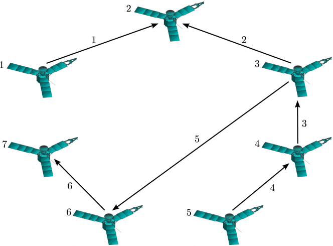
Figure 2: A network of seven satellites with an oriented interaction graph.

Figures 3-6 present the simulation results of our proposed distributed hybrid feedback control laws (12)-(13) and (23)-(24). Since the initial conditions belong to the jump set, the variables $\xi_{k}$ (for both proposed hybrid controllers), for every $k\in\mathcal{M}$, at $t=0$, jump from 0 to $0.9\pi$ and then converge to zero as $t\rightarrow\infty$. Furthermore, the states $\bar{R}_{k}$ and $\omega_{i}$, for every $k\in\mathcal{M}$ and $i\in\mathcal{V}$, also converge to zero as $t\rightarrow\infty$ for both controllers. Simulation videos can be found at https://youtu.be/VViBrnqnkns.

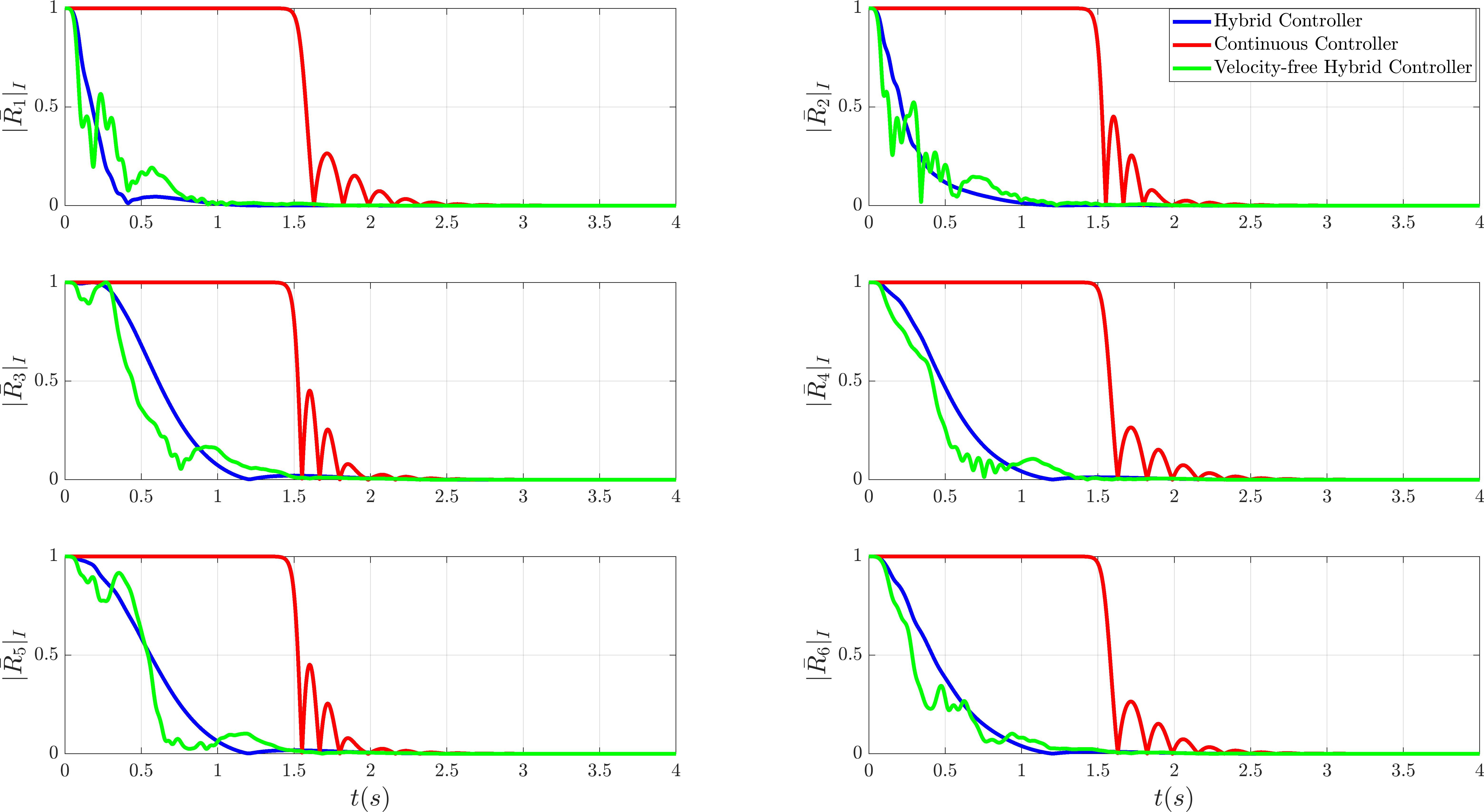
Figure 3: The time evolution of the relative attitude associated with each edge.

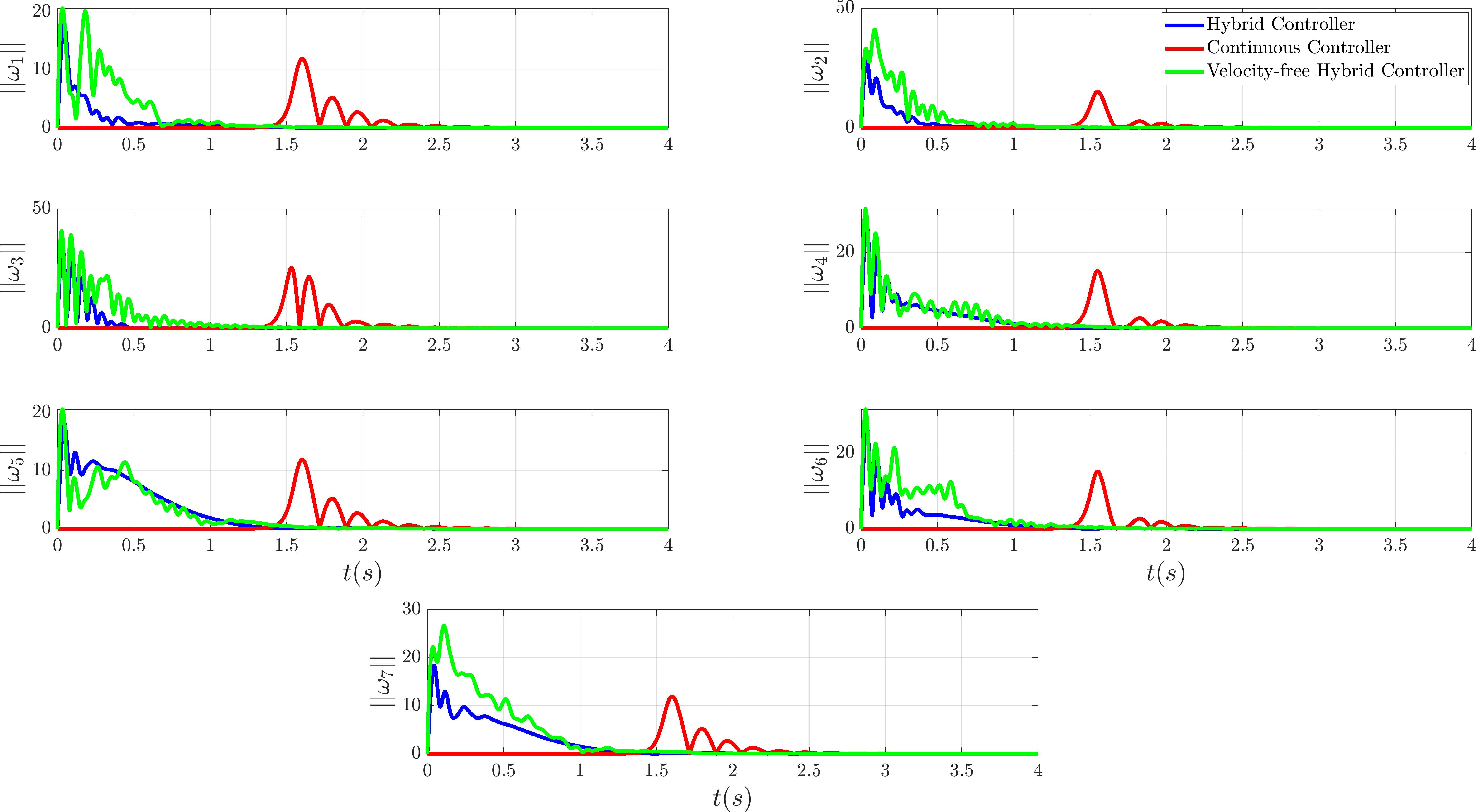
Figure 4: The time evolution of the angular velocity of each agent.

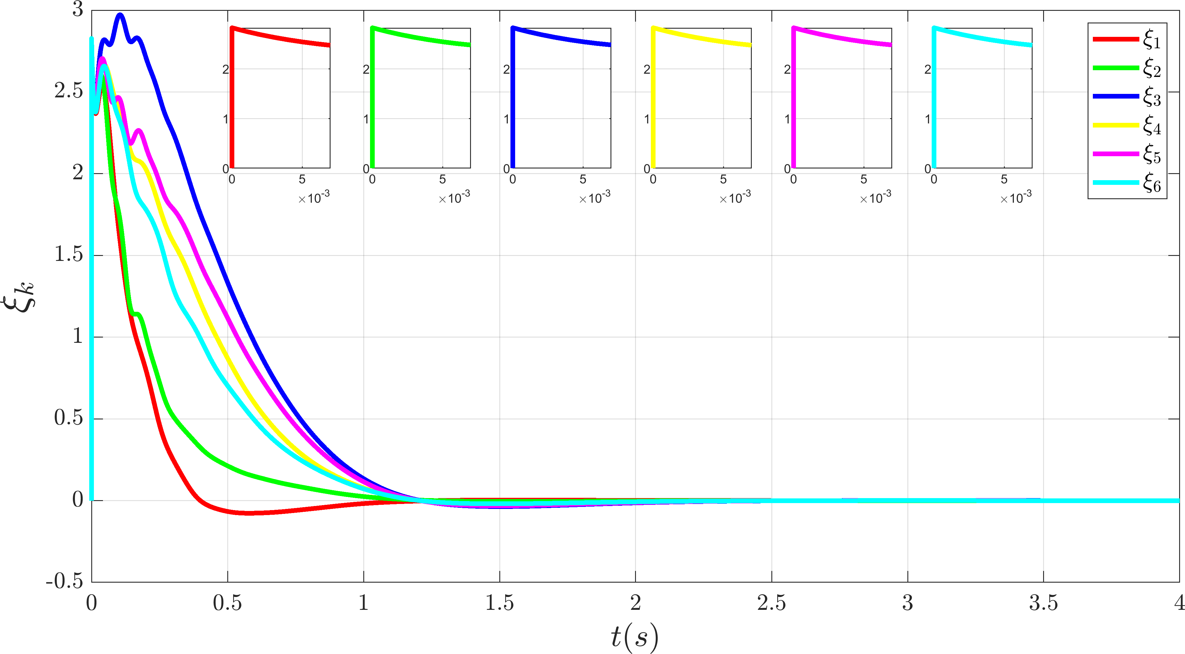
Figure 5: The time evolution of the auxiliary variable $\xi_{k}$ associated with each edge considering Hybrid Controller.

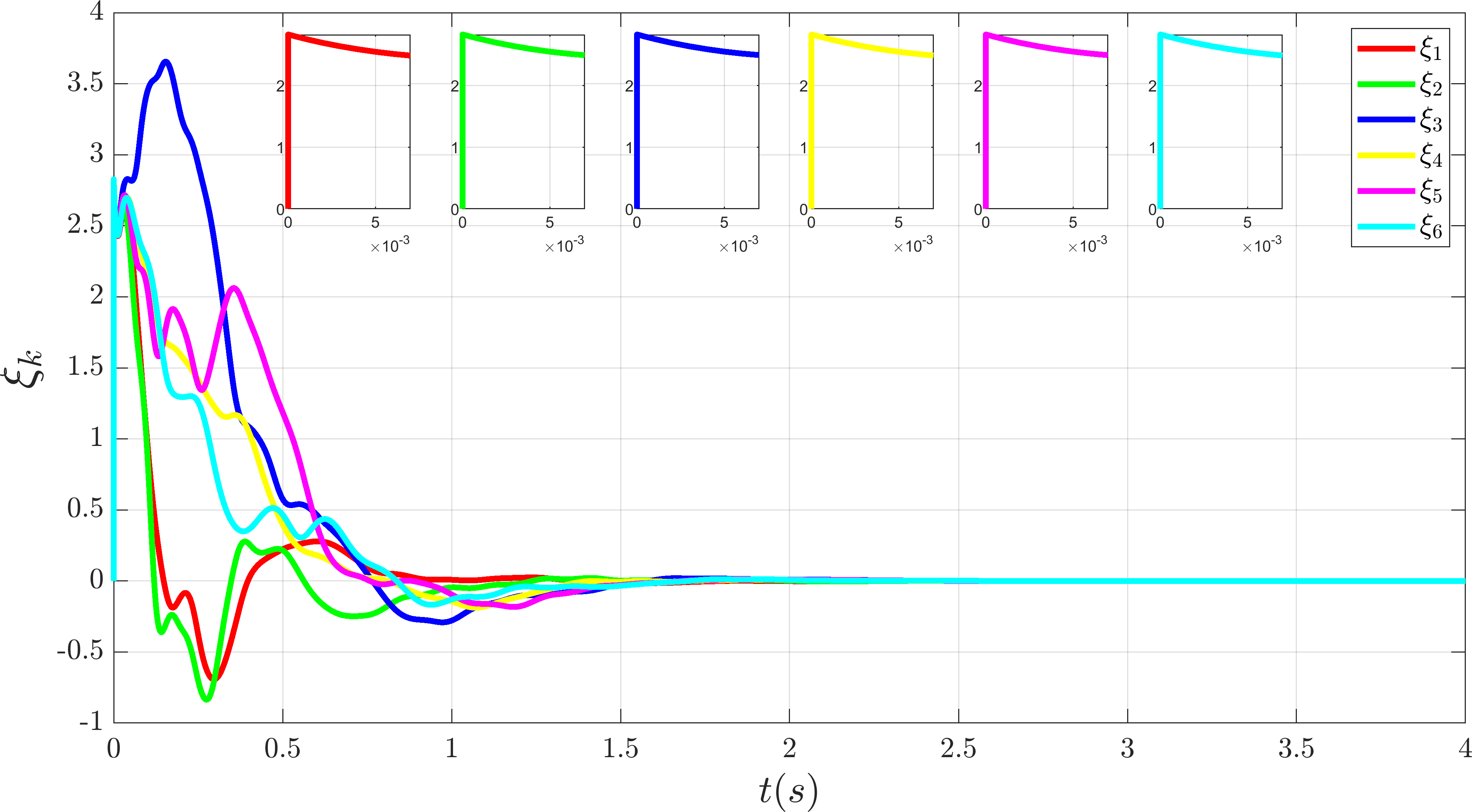
Figure 6: The time evolution of the auxiliary variable $\xi_{k}$ associated with each edge Velocity-free Hybrid Controller.

IX CONCLUSIONS

We have presented three attitude synchronization schemes for rigid body systems on $SO(3)$ under undirected, connected, and acyclic communication graph topology. The first continuous distributed attitude synchronization scheme is quite similar to the scheme proposed in [29], where only local asymptotic stability was claimed. We provided a rigorous proof certifying that this scheme actually enjoys almost global asymptotic stability—the strongest result that one can aim at with smooth control inputs due to the motion space topology involving $SO(3)$. The almost global asymptotic stability result is due to the existence of a finite set of unstable undesired equilibria with a stable manifold of zero Lebesgue measure. To overcome this problem and achieve global asymptotic synchronization, we proposed a new distributed hybrid feedback control scheme on $SO(3)$, relying on angular velocity measurements and relative attitude information, guaranteeing global convergence of the individual orientations to a common orientation. Furthermore, a velocity-free distributed hybrid attitude synchronization scheme on $SO(3)$, with global asymptotic stability guarantees, relying only on attitude measurements, has been proposed. The proposed velocity-free control law uses an auxiliary dynamical system for each agent to generate the necessary damping that compensates for the lack of angular velocity information. Note that both proposed hybrid distributed attitude synchronization schemes have been designed under the assumption that the inter-agent interaction topology is fixed with no communication time delays. Unfortunately, this is not the case in many real-world multi-agent application scenarios. Therefore, redesigning our proposed schemes for multi-agent rigid body systems under dynamically changing and delayed inter-agent communication topology is an interesting future work.

Appendix A Proof of Theorem 1

Considering the undirected graph $\mathcal{G}$ with a virtual (arbitrary) orientation, one has $\mathcal{N}_{i}=\mathcal{I}_{i}\cup\mathcal{O}_{i}$, with $\mathcal{I}_{i}:=\{j\in\mathcal{N}_{i}:j\hskip 2.84544pt\text{is the tail of the oriented edge}\hskip 2.84544pt(i,j)\in\mathcal{E}\}$ and $\mathcal{O}_{i}:=\{j\in\mathcal{N}_{i}:j\hskip 2.84544pt\text{is the head of the oriented edge}\hskip 2.84544pt(i,j)\in\mathcal{E}\}$. From this, one can rewrite the first term of (4) as follows

$$\sum_{j\in\mathcal{N}_{i}}\psi(AR_{j}^{\top}R_{i}) =\sum_{j\in\mathcal{I}_{i}}\psi(AR_{j}^{\top}R_{i})+\sum_{j\in\mathcal{O}_{i}}\psi(AR_{j}^{\top}R_{i})$$

$$=\sum_{j\in\mathcal{I}_{i}}\psi(AR_{j}^{\top}R_{i})-\sum_{j\in\mathcal{O}_{i}}\psi(R_{i}^{\top}R_{j}A)$$ (31)

$$=\sum_{j\in\mathcal{I}_{i}}\psi(AR_{j}^{\top}R_{i})-\sum_{j\in\mathcal{O}_{i}}R_{i}^{\top}R_{j}\psi(AR_{i}^{\top}R_{j})$$ (32)

$$=\sum_{n\in\mathcal{M}_{i}^{+}}\psi(A\bar{R}_{n})-\sum_{l\in\mathcal{M}_{i}^{-}}\bar{R}_{l}\psi(A\bar{R}_{l})$$

$$=\sum_{k=1}^{M}H_{ik}\psi(A\bar{R}_{k}),$$ (33)

where $H_{ik}$ is given in (8). Equations (31) and (32) are obtained using the facts that $\psi(BR)=-\psi(R^{T}B)$ and $\psi(GR)=R^{T}\psi(RG)$, $\forall G,B=B^{T}\in\mathbb{R}^{3\times 3}$ and $R\in SO(3)$. Let $\tau:=[\tau_{1}^{\top},\tau_{2}^{\top},\ldots,\tau_{N}^{\top}]^{\top}\in\mathbb{R}^{3N}$. one can derive the following compact form for the control torque (4):

$$\tau=-k_{R}\bar{H}\Psi-k_{\omega}\omega-\bar{k}_{\omega}(\mathcal{L}\otimes I_{3})\omega,$$ (34)

where $\Psi:=\left[\psi(A\bar{R}_{1})^{\top},\psi(A\bar{R}_{2})^{\top},\ldots,\psi(A\bar{R}_{M})^{\top}\right]^{\top}\in\mathbb{R}^{3M}$ and $\mathcal{L}:=HH^{\top}\in\mathbb{R}^{N\times N}$ is the Laplacian matrix corresponding to the graph $\mathcal{G}$ and the matrix $H$ is given in (II-B). Furthermore, the compact form for the angular velocity dynamics can be written as follows:

$$\mathbf{J}\dot{\omega}=-\mathbf{W}^{\times}\mathbf{J}\omega-k_{R}\bar{H}\Psi-k_{\omega}\omega-\bar{k}_{\omega}(\mathcal{L}\otimes I_{3})\omega,$$ (35)

where $\mathbf{W}^{\times}=:\text{diag}([\omega_{1}]^{\times},[\omega_{2}]^{\times},\ldots,[\omega_{N}]^{\times})\in\mathbb{R}^{3N\times 3N}$ and $\mathbf{J}:=\text{diag}(J_{1},J_{2},\ldots,J_{N})\in\mathbb{R}^{3N\times 3N}$. Now, let us proceed with the stability analysis for the dynamics (5)-(6) with control torque (4). Consider the following Lyapunov function candidate:

$$\mathcal{V}_{z}(z)=\sum_{k=1}^{M}\text{tr}\left(A(I_{3}-\bar{R}_{k})\right)+\omega^{\top}\mathbf{J}\omega.$$ (36)

This Lyapunov function candidate is positive definite on $\mathcal{S}_{z}$ with respect to $\mathcal{A}_{z}$. The time-derivative of $\mathcal{V}_{z}(z)$, along the trajectories of the closed-loop system (5) and (35), is given by

$$\dot{\mathcal{V}}_{z}(z)=-2k_{\omega}||\omega||^{2}-2\bar{k}_{\omega}||(H^{\top}\otimes I_{3})\omega||^{2}.$$ (37)

The last equality was obtained using the facts that $\text{tr}\left(B[x]^{\times}\right)=\text{tr}\left(\mathbb{P}_{a}(B)[x]^{\times}\right)$, $\text{tr}\left([x]^{\times}[y]^{\times}\right)=-2x^{T}y$, $\forall x,y\in\mathbb{R}^{3}$ and $\forall B\in\mathbb{R}^{3\times 3}$ and $\omega^{\top}(\mathcal{L}\otimes I_{3})\omega=||(H^{\top}\otimes I_{3})\omega||^{2}$. The equality (37) shows that the desired equilibrium set $\mathcal{A}_{z}$ is stable. Moreover, as per LaSalle’s invariance theorem, any solution $z$ to the dynamics (5)-(6) with (4), $\forall i\in\mathcal{V}$, must converge to the largest invariant set contained in the set characterized by $\dot{\mathcal{V}}_{z}(z)=0$, i.e., $\omega=0$. From (35), it follows that $\bar{H}\Psi=0$. Applying [48, Lemma 2], the last equality implies $\Psi=0$, which further leads to

$$A\bar{R}_{k}=\bar{R}_{k}^{T}A,$$ (38)

for all $k\in\mathcal{M}$. From (38), we can deduce that $\mathcal{A}_{z}\subset\Upsilon_{z}$. Furthermore, by employing similar arguments to those presented in [41, Lemma 2], every solution $z$ of the dynamics (5)-(6) with (4), $\forall i\in\mathcal{V}$, must converge to the set $\Upsilon_{z}$. This concludes the proof of item (i).

We will now demonstrate the instability of the set of undesired equilibrium points, denoted by $\Upsilon_{z}\setminus\mathcal{A}_{z}$. Before proceeding, we first establish that the set of critical points of the potential function (36) coincides with the set of equilibrium points of the dynamics described by (5)-(6) under the control torque given in (4). To verify this, we will compute the gradient of the potential function $\mathcal{V}_{z}$ with respect to $\bar{R}_{k}$ and $\omega_{i}$ for all $k\in\mathcal{M}$ and $i\in\mathcal{V}$. Let $\mathbb{O}\subset\mathbb{R}$ be an open interval containing zero in its interior. For each $k\in\mathcal{M}$ and $i\in\mathcal{V}$, we define the two smooth curves $\varphi_{k}:\mathbb{O}\to SO(3)$ and $\gamma_{i}:\mathbb{O}\to\mathbb{R}^{3}$ as follows:

$$\varphi_{k}(t) =\bar{R}_{k}\exp\left(t[\zeta_{k}]^{\times}\right)$$ (39)

$$\gamma_{i}(t) =\omega_{i}+v_{i}t,$$ (40)

where $\bar{R}_{k}\in SO(3)$, $\omega_{i}\in\mathbb{R}^{3}$, $\zeta_{k}\in\mathbb{R}^{3}$ and $v_{i}\in\mathbb{R}^{3}$ for every $k\in\mathcal{M}$ and $i\in\mathcal{V}$. Define $\bar{z}(t):=\left(\varphi_{1}(t),\varphi_{2}(t),\ldots,\varphi_{M}(t),\gamma_{1}(t),\gamma_{2}(t),\ldots,\gamma_{N}(t)\right)\in\mathcal{S}_{z}$. The derivative of $\mathcal{V}_{z}\left(\bar{z}(t)\right)$ with respect to $t$ is given by:

$$\frac{d}{dt}\mathcal{V}_{z}\left(\bar{z}(t)\right)= -\sum_{k=1}^{M}\text{tr}\left(A\bar{R}_{k}\exp{\left(t[\zeta_{k}]^{\times}\right)}[\zeta_{k}]^{\times}\right)$$

$$-2\sum_{i=1}^{N}v_{i}^{\top}J_{i}(\omega_{i}+v_{i}t).$$ (41)

Moreover, at $t=0$, one has

$$\left.\frac{d}{dt}\mathcal{V}_{z}\left(\bar{z}(t)\right)\right|_{t=0}= -\sum_{k=1}^{M}\text{tr}\left(A\bar{R}_{k}[\zeta_{k}]^{\times}\right)+2\sum_{i=1}^{N}v_{i}^{\top}J_{i}\omega_{i}$$

$$= 2\sum_{k=1}^{M}\zeta_{k}^{\top}\psi(A\bar{R}_{k})+2\sum_{i=1}^{N}v_{i}^{\top}J_{i}\omega_{i}$$

$$= 2\begin{bmatrix}\zeta^{\top}&v^{\top}\end{bmatrix}^{\top}\begin{bmatrix}\Psi\\ \mathbf{J}\omega\end{bmatrix}.$$ (42)

Note that $\mathbf{J}\omega=\left[\left(\nabla_{\omega_{1}}\mathcal{V}_{z}\right)^{\top},\left(\nabla_{\omega_{2}}\mathcal{V}_{z}\right)^{\top},\ldots,\left(\nabla_{\omega_{N}}\mathcal{V}_{z}\right)^{\top}\right]^{\top}$ $\in\mathbb{R}^{3N}$ and $\Psi=\Bigg{[}\psi\left(\bar{R}^{\top}_{1}\nabla_{\bar{R}_{1}}\mathcal{V}_{z}\right)^{\top},\psi\left(\bar{R}^{\top}_{2}\nabla_{\bar{R}_{2}}\mathcal{V}_{z}\right)^{\top},\ldots,$ $\psi\left(\bar{R}^{\top}_{M}\nabla_{\bar{R}_{M}}\mathcal{V}_{z}\right)^{\top}\Bigg{]}^{\top}$ $\in\mathbb{R}^{3M}$, where $\nabla_{\bar{R}_{k}}\mathcal{V}_{z}$ and $\nabla_{\omega_{i}}\mathcal{V}_{z}$ are the gradients of $\mathcal{V}_{z}$ with respect to $\bar{R}_{k}$ and $\omega_{i}$, respectively, according to the Riemannian metrics $\langle\eta_{1},\eta_{2}\rangle_{SO(3)}=\frac{1}{2}\operatorname{tr}(\eta_{1}^{\top}\eta_{2})$ and $\langle y_{1},y_{2}\rangle_{\mathbb{R}^{3}}=y_{1}^{\top}y_{2}$ for every $\eta_{1},\eta_{2}\in\mathfrak{so}(3)$ and $y_{1},y_{2}\in\mathbb{R}^{3}$. The critical points of the potential function $\mathcal{V}_{z}$ are given by the set $\{z\in\mathcal{S}_{z}:\Psi=0,\omega=0\}$, which corresponds exactly to the set of equilibria $\Upsilon_{z}$ of the dynamics (5)-(6) under the control torque (4). To proceed with the proof of the instability of the set of undesired equilibria $\Upsilon_{z}\setminus\mathcal{A}_{z}$, we evaluate the Hessian of $\mathcal{V}_{z}(z)$, denoted as $\text{{Hess}}\,\mathcal{V}_{z}(z)$, to analyze the nature of the critical points of $\mathcal{V}_{z}(z)$ that lie in the set $\Upsilon_{z}\setminus\mathcal{A}_{z}$. Consider the two smooth curves defined in (39) and (40), where $\bar{R}_{k}=\bar{R}^{*}_{k}$ and $\omega_{i}=\omega_{i}^{*}$ with $(\bar{R}^{*}_{1},\bar{R}^{*}_{2},\ldots,\bar{R}^{*}_{M},\omega^{*}_{1},\omega^{*}_{2},\ldots,\omega^{*}_{N})\in\Upsilon_{z}\setminus\mathcal{A}_{z}$. The second derivative of $\mathcal{V}_{z}(\bar{z})$ with respect to $t$ is given by:

$$\frac{d^{2}}{dt^{2}}\mathcal{V}_{z}(\bar{z})= -\sum_{k=1}^{M}\text{tr}\left(A\bar{R}^{*}_{k}\exp{\left(t[\zeta_{k}]^{\times}\right)}\left([\zeta_{k}]^{\times}\right)^{2}\right)$$

$$-\sum_{k=1}^{M}\text{tr}\left(A\bar{R}^{*}_{k}\exp{\left(t[\zeta_{k}]^{\times}\right)}[\dot{\zeta}_{k}]^{\times}\right)+\sum_{i=1}^{N}v_{i}^{\top}J_{i}v_{i}$$

$$+\sum_{i=1}^{N}\dot{v}_{i}^{\top}J_{i}(\omega^{*}_{i}+v_{i}t).$$ (43)

Given that $\mathbb{P}_{a}(A\bar{R}^{*}_{k})=0$ and $\omega_{i}^{*}=0$ for all $(\bar{R}^{*}_{1},\bar{R}^{*}_{2},\ldots,\bar{R}^{*}_{M},\omega^{*}_{1},\omega^{*}_{2},\ldots,\omega^{*}_{N})\in\Upsilon_{z}\setminus\mathcal{A}_{z}$, it follows that

$$\left.\frac{d^{2}}{dt^{2}}\mathcal{V}_{z}(\bar{z})\right|_{t=0}= -\sum_{k=1}^{M}\text{tr}\left(A\bar{R}^{*}_{k}\left([\zeta_{k}]^{\times}\right)^{2}\right)+\sum_{i=1}^{N}v_{i}^{\top}J_{i}v_{i}.$$ (44)

Using the identity $\left([\zeta]^{\times}\right)^{2}=-\|\zeta\|^{2}I_{3}+\zeta\zeta^{T}$ and the property $\text{tr}(\zeta_{1}\zeta_{2}^{T})=\zeta_{1}^{T}\zeta_{2}$ for all $\zeta,\zeta_{1},\zeta_{2}\in\mathbb{R}^{3}$, we further simplify equation (44) as follows:

$$\left.\frac{d^{2}}{dt^{2}}\mathcal{V}_{z}(\bar{z})\right|_{t=0}\!= \sum_{k=1}^{M}\zeta^{\top}_{k}\left(\text{tr}(A\bar{R}^{*}_{k})I_{3}-A\bar{R}^{*}_{k}\right)\zeta_{k}+\sum_{i=1}^{N}v_{i}^{\top}J_{i}v_{i}$$

$$=\sum_{k=1}^{M}\zeta^{T}_{k}A^{*}_{k}\zeta_{k}+\sum_{i=1}^{N}v_{i}^{\top}J_{i}v_{i},$$ (45)

where $A^{*}_{k}=\text{tr}(A\bar{R}^{*}_{k})I_{3}-A\bar{R}^{*}_{k}$. Letting $\mathbf{A}^{*}=\text{diag}(A^{*}_{1},A^{*}_{2},\ldots,A^{*}_{M})\in\mathbb{R}^{3M\times 3M}$, $\zeta=[\zeta_{1}^{\top},\zeta_{2}^{\top},\ldots,\zeta_{M}^{\top}]^{\top}\in\mathbb{R}^{3M}$ and $v=[v_{1}^{\top},v_{2}^{\top},\ldots,v_{N}^{\top}]^{\top}\in\mathbb{R}^{3N}$, one has

$$\left.\frac{d^{2}}{dt^{2}}\mathcal{V}_{z}(\bar{z})\right|_{t=0}\! =\zeta^{\top}\mathbf{A}^{*}\zeta+v^{\top}\mathbf{J}v$$

$$=\begin{bmatrix}\zeta^{\top}&v^{\top}\end{bmatrix}^{\top}\begin{pmatrix}\mathbf{A}^{*}&0_{3M\times 3N}\\ 0_{3N\times 3M}&\mathbf{J}\end{pmatrix}\begin{bmatrix}\zeta\\ v\end{bmatrix}.$$ (46)

It follows from (A) that

$$\text{{Hess}}\,\mathcal{V}_{z}(z)=\begin{pmatrix}\mathbf{A}^{*}&0_{3M\times 3N}\\ 0_{3N\times 3M}&\mathbf{J}\end{pmatrix},$$ (47)

for every $z\in\Upsilon_{z}\setminus\mathcal{A}_{z}$. The matrix (47) represents the Hessian of $\mathcal{V}_{z}$ evaluated at the critical points on $\Upsilon_{z}\setminus\mathcal{A}_{z}$. Note that $\text{{Hess}}\,\mathcal{V}_{z}(z)$ is a block diagonal matrix. To determine whether the critical points on $\Upsilon_{z}\setminus\mathcal{A}_{z}$ are minima, maxima, or saddle points, it is essential to analyze the eigenvalues of the matrices $\mathbf{A}^{*}$ and $\mathbf{J}$. Given that the matrix $\mathbf{J}$ is positive definite, the focus should be on evaluating the eigenvalues of $\mathbf{A}^{*}$. Since $\mathbf{A}^{*}=\text{diag}(A^{*}_{1},A^{*}_{2},\ldots,A^{*}_{M})$, we will explicitly determine the eigenvalues of the matrices $A^{*}_{k}$ for every $k\in\mathcal{M}$. According to the set $\Upsilon_{z}\setminus\mathcal{A}_{z}$, we have $A_{m}^{*}=\text{tr}(A)-A$ and $A_{n}^{*}\in\{{}^{1}A_{n},{}^{2}A_{n},{}^{3}A_{n}\}$ for every $m\in\mathcal{M}^{I}$ and $n\in\mathcal{M}^{\pi}$, where the matrix ${}^{\beta_{n}}A_{n}$ can be calculated as follows:

$${}^{\beta_{n}}A_{n}= \text{tr}\left(A\mathcal{R}(\pi,u_{\beta_{n}})\right)I_{3}-A\mathcal{R}(\pi,u_{\beta_{n}}),$$ (48)

where $u_{\beta_{n}}\in\mathcal{E}(A)$. Using the fact that $\mathcal{R}(\pi,u_{\beta_{n}})=-I_{3}+2u_{\beta_{n}}u_{\beta_{n}}^{\top}$, it follows from (48) that

$${}^{\beta_{n}}A_{n}=-\text{tr}(A)I_{3}+2\lambda_{\beta_{n}}I_{3}+A-2\lambda_{\beta_{n}}u_{\beta_{n}}u_{\beta_{n}}^{\top},$$

where $\lambda_{\beta_{n}}$ is the eigenvalue of $A$ corresponding to the eigenvector $u_{\beta_{n}}$ for each $\beta_{n}\in\{1,2,3\}$. Note that, for each $n\in\mathcal{M}^{\pi}$, the matrix $A_{n}^{*}$ can take one of three possible values (i.e., ${}^{1}A_{n},{}^{2}A_{n}$ or ${}^{3}A_{n}$), depending on the choice of the eigenvector of the matrix $A$. The set of eigenpairs of the matrix $A_{m}^{*}$ is given by

$$\left\{(\lambda_{2}+\lambda_{3},u_{1}),(\lambda_{1}+\lambda_{3},u_{2}),(\lambda_{1}+\lambda_{2},u_{3})\right\},$$

for all $m\in\mathcal{M}^{I}$. For the matrices ${}^{1}A_{n}$, ${}^{2}A_{n}$, and ${}^{3}A_{n}$, the eigenpair sets are found to be:

• For ${}^{1}A_{n}$:

  $$\{(-\lambda_{2}-\lambda_{3},u_{1}),(\lambda_{1}-\lambda_{3},u_{2}),(\lambda_{1}-\lambda_{2},u_{3})\},$$

• For ${}^{2}A_{n}$:

  $$\{(\lambda_{2}-\lambda_{3},u_{1}),(-\lambda_{1}-\lambda_{3},u_{2}),(\lambda_{2}-\lambda_{1},u_{3})\},$$

• For ${}^{3}A_{n}$:

  $$\{(\lambda_{3}-\lambda_{2},u_{1}),(\lambda_{3}-\lambda_{1},u_{2}),(-\lambda_{1}-\lambda_{2},u_{3})\},$$

for all $n\in\mathcal{M}^{\pi}$. It follows from the fact that $\lambda_{1}>\lambda_{2}>\lambda_{3}$, the eigenvalues of $A^{*}_{k}$ must either be all negative or contain a mixture of positive and negative values. Combined with the fact that the matrix $\mathbf{J}$ is positive definite, this indicates that the critical points of $\mathcal{V}_{z}(z)$ within $\Upsilon_{z}\setminus\mathcal{A}_{z}$ are saddle points of $\mathcal{V}_{z}(z)$. Now, we are ready to show the instability of undesired equilibrium points $\Upsilon_{z}\setminus\mathcal{A}_{z}$ for the dynamics (5)-(6) with the control torque (4). Consider the real-valued function $\bar{\mathcal{V}}_{z}(z):SO(3)^{M}\times\mathbb{R}^{3N}\rightarrow\mathbb{R}$, defined as follows:

$$\bar{\mathcal{V}}_{z}(z)=2\sum_{n\in\mathcal{M}^{\pi}}(\lambda_{p_{n}}+\lambda_{d_{n}})-\mathcal{V}_{z}(z),$$ (49)

where $\lambda_{p_{n}}$ and $\lambda_{d_{n}}$ are two distinct eigenvalues of the matrix $A$, i.e., $p_{n},d_{n}\in\{1,2,3\}$ with $p_{n}\neq d_{n}$. Let $z^{*}\in\Upsilon_{z}\setminus\mathcal{A}_{z}$ denote an undesired equilibrium point such that $\bar{R}_{n}=\mathcal{R}(\pi,u_{l_{n}})$ for $n\in\mathcal{M}^{\pi}$, where $l_{n}\in\{1,2,3\}$ satisfies $l_{n}\neq p_{n}$ and $l_{n}\neq d_{n}$. Clearly, $\bar{\mathcal{V}}_{z}(z^{*})=0$. Define the set $\mathbb{B}_{r}:=\{(\bar{R}_{1},\bar{R}_{2},\dots,\bar{R}_{M},\omega_{1},\omega_{2},\dots,\omega_{N})\in\mathcal{S}_{z}:|\bar{R}_{1}^{\top}\bar{R}_{1}^{*}|_{I}+|\bar{R}_{2}^{\top}\bar{R}_{2}^{*}|_{I}+\dots+|\bar{R}_{M}^{\top}\bar{R}_{M}^{*}|_{I}+||\omega_{1}||+||\omega_{2}||+\dots+||\omega_{N}||\leq r\}$ with $r>0$. Since the set $\Upsilon_{z}\setminus\mathcal{A}_{z}$ consists only the saddle points of $\bar{\mathcal{V}}(z)$, it follows that the set $\mathbb{U}=\{z\in\mathbb{B}_{r}\mid\bar{\mathcal{V}}(z)>0\}$ is non-empty. Moreover, in view of (37) and (49), one has that $\dot{\bar{\mathcal{V}}}(z)=-\dot{\mathcal{V}}(z)>0$ in $\mathbb{U}$, which implies that any trajectory originating in the set $\mathbb{U}$ must exit $\mathbb{U}$. By virtue of Chetaev’s theorem [49], it can be concluded that all points in the undesired equilibrium set $\Upsilon_{z}\setminus\mathcal{A}_{z}$ are unstable. Additionally, by the stable manifold theorem [50] and the fact that the vector field given in the dynamics (5)-(6) under the continuous control torque (4) is at least $C^{1}$, the stable manifold associated with the undesired equilibrium set $\Upsilon\setminus\mathcal{A}$ has zero Lebesgue measure. Consequently, the equilibrium set $\mathcal{A}$ is almost globally asymptotically stable. This completes the proof of item (ii) and item (1).

Appendix B Proof of Theorem 2

In view of (6) and (12), one can verify that

$$\mathbf{J}\dot{\omega}=-k^{R}\bar{H}~\Psi_{\nabla}^{\bar{R}}-k_{\omega}\omega-\bar{k}_{\omega}(\mathcal{L}\otimes I_{3})\omega,$$ (50)

where $\Psi_{\nabla}^{\bar{R}}:=\Bigg{[}\psi\left(\bar{R}^{\top}_{1}\nabla_{\bar{R}_{1}}U_{T}\right)^{\top},\psi\left(\bar{R}^{\top}_{2}\nabla_{\bar{R}_{2}}U_{T}\right)^{\top},\ldots,$ $\psi\left(\bar{R}^{\top}_{M}\nabla_{\bar{R}_{M}}U_{T}\right)^{\top}\Bigg{]}^{\top}\in\mathbb{R}^{3M}$, $\mathbf{J}:=\text{diag}(J_{1},J_{2},\ldots,J_{N})\in\mathbb{R}^{3N\times 3N}$, $\mathcal{L}:=HH^{\top}\in\mathbb{R}^{N\times N}$ is the Laplacian matrix corresponding to the graph $\mathcal{G}$ and the matrix $\bar{H}$ is given in (8). Consider the following Lyapunov function candidate:

$$\mathcal{V}(\bar{x})= k_{R}\bar{U}(x)+\omega^{\top}\mathbf{J}\omega.$$ (51)

Note that $\mathcal{V}$ is positive definite on $\bar{\mathcal{S}}$ with respect to $\bar{\mathcal{A}}$. The time-derivative of $\mathcal{V}$, along the trajectories generated by the flows of the hybrid closed-loop dynamics (14), is given by

$$\dot{\mathcal{V}}(\bar{x})=k_{R}\dot{\bar{U}}(x)+2\omega^{\top}\mathbf{J}\dot{\omega}.$$ (52)

The time-derivative of the first term of (52) can be calculated as follows

$$\dot{\bar{U}}(x)= \sum_{k=1}^{M}\langle\nabla_{\bar{R}_{k}}\bar{U},\bar{R}_{k}[\bar{\omega}_{k}]^{\times}\rangle_{\bar{R}_{k}}+\sum_{k=1}^{M}\langle\langle\nabla_{\xi_{k}}\bar{U},\dot{\xi}_{k}\rangle\rangle$$

$$= \sum_{k=1}^{M}\langle\langle\bar{R}_{k}^{\top}\nabla_{\bar{R}_{k}}\bar{U},[\bar{\omega}_{k}]^{\times}\rangle\rangle+\sum_{k=1}^{M}\langle\langle\nabla_{\xi_{k}}\bar{U},\dot{\xi}_{k}\rangle\rangle$$

$$= 2\sum_{k=1}^{M}\bar{\omega}_{k}^{\top}\psi\left(\bar{R}^{\top}_{k}\nabla_{\bar{R}_{k}}\bar{U}\right)+\sum_{k=1}^{M}\dot{\xi}_{k}\nabla_{\xi_{k}}\bar{U}$$ (53)

$$= 2~\bar{\omega}^{\top}\Psi_{\nabla}^{\bar{R}}+\dot{\xi}^{\top}\Psi_{\nabla}^{\xi}=2~\omega^{\top}\bar{H}\Psi_{\nabla}^{\bar{R}}-k_{\xi}||\Psi_{\nabla}^{\xi}||^{2},$$ (54)

where $\Psi_{\nabla}^{\xi}:=\left[\nabla_{\xi_{1}}\bar{U},\nabla_{\xi_{2}}\bar{U},\ldots,\nabla_{\xi_{M}}\bar{U}\right]^{\top}\in\mathbb{R}^{M}$. To derive the above equations, the following identities have been used: $\langle\eta_{1},\eta_{2}\rangle_{R}=\langle\langle R^{\top}\eta_{1},R^{\top}\eta_{2}\rangle\rangle$, $\text{tr}\left(B[x]^{\times}\right)=\text{tr}\left(\mathbb{P}_{a}(B)[x]^{\times}\right)$ and $\text{tr}\left([x]^{\times}[y]^{\times}\right)=-2x^{\top}y$, $\forall x,y\in\mathbb{R}^{3}$, $\forall B\in\mathbb{R}^{3\times 3}$, $\forall\eta_{1},\eta_{2}\in\mathfrak{so}(3)$ and $\forall R\in SO(3)$. Furthermore, from (6), (12) and (54), one obtains the following time-derivative of $\mathcal{V}(\bar{x})$

$$\dot{\mathcal{V}}(\bar{x})= -k_{R}k_{\xi}||\Psi_{\nabla}^{\xi}||^{2}-2k_{\omega}||\omega||^{2}-2\bar{k}_{\omega}||(H^{\top}\otimes I_{3})\omega||^{2},$$ (55)

which implies that $\mathcal{V}$ is non-increasing along the flows of (14). Moreover, in view of (14) and (51), one has

$$\mathcal{V}(\bar{x})-\mathcal{V}(\bar{x}^{+})= k_{R}\left(\bar{U}(x)-\bar{U}(x^{+})\right)$$

$$= k_{R}\sum_{k=1}^{M}\left(U(\bar{R}_{k},\xi_{k})-U(\bar{R}_{k}^{+},\xi_{k}^{+})\right)$$

$$\geq k_{R}\delta_{\bar{R}},$$ (56)

which indicates that $\mathcal{V}(\bar{x})$ is strictly decreasing over the jumps of (14). In view of (55) and (B), it follows that set $\bar{\mathcal{A}}$ is stable [38, Theorem 23], and hence all maximal solutions of (14) are bounded. From (55) and (B), one can also verify that $\mathcal{V}(\bar{x}(t,j))\leq\mathcal{V}(\bar{x}(t_{j},j))$ and $\mathcal{V}(\bar{x}(t_{j},j))\leq\mathcal{V}(\bar{x}(t_{j},j-1))-k_{R}\delta_{\bar{R}}$, $\forall(t,j),(t_{j},j),(t_{j},j-1)\in\text{dom}~\bar{x}$, with $(t,j)\geq(t_{j},j)\geq(t_{j},j-1)$. Thus, one has $0\leq\mathcal{V}(\bar{x}(t,j))\leq\mathcal{V}(\bar{x}(0,0))-jk_{R}$, $\forall(t,j)\in\text{dom}~\bar{x}$, which leads to $j\leq\lceil\frac{\mathcal{V}(\bar{x}(0,0))}{k_{R}\delta_{\bar{R}}}\rceil$, where $\lceil.\rceil$ denotes the ceiling function. The last inequality implies that the number of jumps is finite and depends on the initial conditions.
Next, using the invariance principle for hybrid systems [39, Section 8.2], we will demonstrate the global attractivity of $\bar{\mathcal{A}}$. Defining the following functions:

$$u_{\bar{\mathcal{F}}}(\bar{x}) :=\begin{cases}-k_{R}k_{\xi}||\Psi_{\nabla}^{\xi}||^{2}-2k_{\omega}||\omega||^{2}-2\bar{k}_{\omega}||(H^{\top}\otimes I_{3})\omega||^{2}\\ ~~~~~~~~~~~~~~~~~~~~~~~\text{if}~\bar{x}\in\bar{\mathcal{F}},\\ -\infty~~~~~~~~~~~~\text{otherwise},\end{cases}$$ (57)

$$u_{\bar{\mathcal{J}}}(\bar{x}) :=\begin{cases}&-k_{R}\delta_{\bar{R}}~~~~~~~~~~~~\text{if}~\bar{x}\in\bar{\mathcal{J}},\\ &-\infty~~~~~~~~~~\text{otherwise}.\end{cases}$$ (58)

One verifies that the growth of $\mathcal{V}$ is upper bounded during the flows by $u_{\bar{\mathcal{F}}}(\bar{x})\leq 0$ and during the jumps by $u_{\bar{\mathcal{J}}}(\bar{x})\leq 0$ for every $\bar{x}\in\bar{\mathcal{S}}$. Consequently, according to [39, Corollary 8.4], every maximal solution of the hybrid system (14) converges to the following largest weakly invariant subset:

$$\mathcal{V}^{-1}(r)\cap\bar{\mathcal{S}}\cap\left[\overline{u_{\bar{\mathcal{F}}}^{-1}(0)}\cup\left(u_{\bar{\mathcal{J}}}^{-1}(0)\cap\bar{G}\left(u_{\bar{\mathcal{J}}}^{-1}(0)\right)\right)\right],$$

for some $r\in\mathbb{R}$, where $\overline{u_{\bar{\mathcal{F}}}^{-1}(0)}$ denotes the closure of the set $u_{\bar{\mathcal{F}}}^{-1}(0)$. For $k_{\omega}>0$, one can verify that

$$u_{\bar{\mathcal{F}}}^{-1}(0) =\{\bar{x}\in\bar{\mathcal{F}}:~\Psi_{\nabla}^{\xi}=0,~\omega=0\}$$

$$u_{\mathcal{J}}^{-1}(0) =\emptyset.$$

Since for every $\bar{x}\in u_{\bar{\mathcal{F}}}^{-1}(0)$, one has $\omega=0$, which implies $\dot{\omega}=0$, it follows from (50) that $\bar{H}\Psi_{\nabla}^{\bar{R}}=0$, which further implies, as per [48, Lemma 2], that $\Psi_{\nabla}^{\bar{R}}=0$. Therefore, one can verify that any solution to the hybrid closed-loop system (14) converges to the largest invariant set contained in

$$u_{\bar{\mathcal{F}}}^{-1}(0) =\{\bar{x}\in\bar{\mathcal{F}}:~x\in\mathcal{F}\cap\bar{\Upsilon},~\omega=0\}.$$

On the other hand, given $x\in\mathcal{A}$, one has, for all $k\in\mathcal{M}$, $U(\bar{R}_{k},\xi_{k})-\underset{\bar{\xi}_{k}\in\Xi}{\text{min}}U(\bar{R}_{k},\bar{\xi}_{k})=-\underset{\bar{\xi}_{k}\in\Xi}{\text{min}}U(\bar{R}_{k},\bar{\xi}_{k})\leq 0$. Therefore, from (15), and according to Condition 1, one can verify that $\mathcal{A}\subset\mathcal{F}\cap\bar{\Upsilon}$ and $\mathcal{F}\cap(\bar{\Upsilon}\setminus\mathcal{A})=\varnothing$. In addition, applying some set-theoretic arguments, one has $\mathcal{F}\cap\bar{\Upsilon}\subset(\mathcal{F}\cap(\bar{\Upsilon}\setminus\mathcal{A}))\cup(\mathcal{F}\cap\mathcal{A})=\varnothing\cup\mathcal{A}$. It follows from $\mathcal{A}\subset\mathcal{F}\cap\bar{\Upsilon}$ and $\mathcal{F}\cap\bar{\Upsilon}\subset\mathcal{A}$ that $\mathcal{F}\cap\bar{\Upsilon}=\mathcal{A}$. This implies that $u_{\bar{\mathcal{F}}}^{-1}(0)=\bar{\mathcal{A}}$. Hence, every maximal solution of the hybrid system (14) converges to the largest weakly invariant subset $\mathcal{V}^{-1}(0)\cap\bar{\mathcal{A}}=\bar{\mathcal{A}}$. Since every maximal solution of the hybrid closed-loop system (14) is bounded, $\bar{G}(\bar{x})\in\bar{\mathcal{F}}\cup\bar{\mathcal{J}}$ for every $\bar{x}\in\bar{\mathcal{J}}$, and $\bar{F}(\bar{x})\subset T_{\bar{\mathcal{F}}}(\bar{x})$, for every $\bar{x}\in\bar{\mathcal{F}}\setminus\bar{\mathcal{J}}$, where $T_{\bar{\mathcal{F}}}(\bar{x})$ denotes the tangent cone to $\bar{\mathcal{F}}$ at the point $\bar{x}$, according to [39, Proposition 6.10], one can conclude that every maximal solution of the hybrid closed-loop system (14) is complete. This, together with Lemma 1, allows us to conclude that the set $\bar{\mathcal{A}}$ is globally asymptotically stable for the hybrid closed-loop system (14). This completes the proof.

Appendix C Proof of Theorem 3

Consider the following Lyapunov function candidate:

$$\hat{\mathcal{V}}(\hat{x})= k_{R}\sum_{i=1}^{M}U(\bar{R}_{k},\xi_{k})+k_{\tilde{Q}}\sum_{i=1}^{N}U(\tilde{Q}_{i},\zeta_{i})+\sum_{i=1}^{N}\omega_{i}^{\top}J_{i}\omega_{i}.$$ (59)

One can verify that the above Lyapunov function candidate is positive definite on $\hat{\mathcal{S}}$ with respect to $\hat{\mathcal{A}}$, and its time-derivative, along the trajectories generated by the flows of the hybrid closed-loop dynamics (26), is given by

$$\dot{\hat{\mathcal{V}}}(\hat{x})=-k_{R}k_{\xi}||\Psi_{\nabla}^{\xi}||^{2}-2k_{\tilde{Q}}k_{Q}||\Psi_{\nabla}^{\tilde{Q}}||^{2}-k_{\tilde{Q}}k_{\zeta}||\Psi_{\nabla}^{\zeta}||^{2},$$ (60)

where $\Psi_{\nabla}^{\tilde{Q}}:=\Bigg{[}\psi\left(\tilde{Q}^{\top}_{1}\nabla_{\tilde{Q}_{1}}U(\tilde{Q}_{1},\zeta_{1})\right)^{\top}\hskip-5.69046pt,\psi\left(\tilde{Q}^{\top}_{2}\nabla_{\tilde{Q}_{2}}U(\tilde{Q}_{2},\zeta_{2})\right)^{\top}$ $,\ldots,\psi\left(\tilde{Q}^{\top}_{N}\nabla_{\tilde{Q}_{N}}U(\tilde{Q}_{N},\zeta_{N})\right)^{\top}\Bigg{]}^{\top}\in\mathbb{R}^{3N}$, $\Psi_{\nabla}^{\zeta}:=\bigg{[}\nabla_{\zeta_{1}}U(\tilde{Q}_{1},\zeta_{1}),\nabla_{\zeta_{2}}U(\tilde{Q}_{2},\zeta_{2}),\ldots,\nabla_{\zeta_{N}}U(\tilde{Q}_{N},\zeta_{N})\bigg{]}^{\top}$ $\in\mathbb{R}^{N}$ and $\zeta:=[\zeta_{1},\zeta_{2},\ldots,\zeta_{N}]^{\top}\in\mathbb{R}^{N}$. This implies that $\hat{\mathcal{V}}$ is non-increasing along the flow of (26). Furthermore, one has

$$\hat{\mathcal{V}}(\hat{x})-\hat{\mathcal{V}}(\hat{x}^{+})= k_{R}\sum_{k=1}^{M}\left(U(\bar{R}_{k},\xi_{k})-U(\bar{R}_{k}^{+},\xi_{k}^{+})\right)$$

$$+k_{\tilde{Q}}\sum_{i=1}^{N}\left(U(\tilde{Q}_{i},\zeta_{i})-U(\tilde{Q}_{i}^{+},\zeta_{i}^{+})\right)$$

$$\geq \underline{k}~\underline{\delta}$$ (61)

where $\underline{k}:=\text{min}\{k_{R},k_{Q}\}$ and $\underline{\delta}:=\text{min}\{\delta_{\bar{R}},\delta_{\tilde{Q}}\}$. Following the same steps as in the proof of Theorem 2, it can be shown that the set $\hat{\mathcal{A}}$ is stable, every maximal solution of the hybrid closed-loop dynamics (26) is complete, and the number of jumps is finite. Furthermore, consider the following two functions:

$$u_{\hat{\mathcal{F}}}(\hat{x}) :=\begin{cases}-k_{R}k_{\xi}||\Psi_{\nabla}^{\xi}||^{2}-2k_{\tilde{Q}}k_{Q}||\Psi_{\nabla}^{\tilde{Q}}||^{2}-k_{\tilde{Q}}k_{\zeta}||\Psi_{\nabla}^{\zeta}||^{2}\\ ~~~~~~~~~~~~~~~~~~~~\text{if}~\hat{x}\in\hat{\mathcal{F}},\\ -\infty~~~~~~~~~~~~\text{otherwise},\end{cases}$$

$$u_{\hat{\mathcal{J}}}(\hat{x}) :=\begin{cases}&-\underline{k}~\underline{\delta}~~~~~~~~~~~~\text{if}~\hat{x}\in\hat{\mathcal{J}},\\ &-\infty~~~~~~~~~~\text{otherwise}.\end{cases}$$ (62)

It follows from the invariance principle for hybrid systems, given in [39, Section 8.2], that every maximal solution of the hybrid system (26) converges to the following largest weakly invariant subset:

$$\hat{\mathcal{V}}^{-1}(r)\cap\hat{\mathcal{S}}\cap\left[\overline{u_{\hat{\mathcal{F}}}^{-1}(0)}\cup\left(u_{\hat{\mathcal{J}}}^{-1}(0)\cap G\left(u_{\hat{\mathcal{J}}}^{-1}(0)\right)\right)\right],$$

for some $r\in\mathbb{R}$, where $u_{\hat{\mathcal{J}}}^{-1}(0)=\emptyset$ and $u_{\hat{\mathcal{F}}}^{-1}(0)=\{\hat{x}\in\hat{\mathcal{F}}:~\Psi_{\nabla}^{\xi}=0,~\Psi_{\nabla}^{\tilde{Q}}=0,~\Psi_{\nabla}^{\zeta}=0\}$. Note that, for every $\hat{x}\in u_{\hat{\mathcal{F}}}^{-1}(0)$, one has $\Psi_{\nabla}^{\xi}=0$ and, for $i\in\mathcal{V}$, $(\tilde{Q}_{i},\zeta_{i})\in\mathcal{F}_{i}^{\tilde{Q}}\cap\Upsilon$. According to [45], along with Condition 2, it can be shown that $\mathcal{F}_{i}^{\tilde{Q}}\cap\Upsilon=\{(I_{3},0)\}$. Moreover, from the fact that $\dot{\tilde{Q}}_{i}=0$ (since $\tilde{Q}_{i}=I_{3}$), one has $\omega_{i}=k_{Q}\psi\left(\tilde{Q}^{\top}_{i}\nabla_{\tilde{Q}_{i}}U(\tilde{Q}_{i},\zeta_{i})\right)=0$. This implies that $k_{R}\bar{H}\Psi_{\nabla}^{\bar{R}}=0$. This fact together with $\Psi_{\nabla}^{\xi}=0$ and considering the last part of the proof of Theorem 2, one has $\bar{x}\in\bar{\mathcal{A}}$. Finally, one concludes that $u_{\hat{\mathcal{F}}}^{-1}(0)=\hat{\mathcal{A}}$ and every maximal solution of the hybrid system (26) converges to the largest weakly invariant subset $\hat{\mathcal{V}}^{-1}(0)\cap\hat{\mathcal{A}}=\hat{\mathcal{A}}$. Combining this with the fact that every maximal solution of the hybrid closed-loop system (26) is complete and (26) satisfies the basic hybrid conditions, implies that the set $\hat{\mathcal{A}}$ is globally asymptotically stable for the hybrid closed-loop system (26). This completes the proof.

References

• [1] M. Boughellaba and A. Tayebi, “Global attitude alignment for multi-agent systems on so(3) without angular velocity measurements,” in 2024 American Control Conference (ACC), 2024, pp. 2041–2046.
• [2] K.-K. Oh and H.-S. Ahn, “Formation control and network localization via orientation alignment,” IEEE Transactions on Automatic Control, vol. 59, no. 2, pp. 540–545, 2014.
• [3] N. Moshtagh, N. Michael, A. Jadbabaie, and K. Daniilidis, “Vision-based, distributed control laws for motion coordination of nonholonomic robots,” IEEE Transactions on Robotics, vol. 25, no. 4, pp. 851–860, 2009.
• [4] D. V. Dimarogonas, P. Tsiotras, and K. J. Kyriakopoulos, “Leader–follower cooperative attitude control of multiple rigid bodies,” Systems & Control Letters, vol. 58, no. 6, pp. 429–435, 2009.
• [5] I. Bayezit and B. Fidan, “Distributed cohesive motion control of flight vehicle formations,” IEEE Transactions on Industrial Electronics, vol. 60, no. 12, pp. 5763–5772, 2013.
• [6] W. Ren, “Distributed cooperative attitude synchronization and tracking for multiple rigid bodies,” IEEE Transactions on Control Systems Technology, vol. 18, no. 2, pp. 383–392, 2010.
• [7] X. Jin, Y. Shi, Y. Tang, and X. Wu, “Event-triggered attitude consensus with absolute and relative attitude measurements,” Automatica, vol. 122, p. 109245, 2020.
• [8] Z. Meng, W. Ren, and Z. You, “Distributed finite-time attitude containment control for multiple rigid bodies,” Automatica, vol. 46, no. 12, pp. 2092–2099, 2010.
• [9] T. Chen, J. Shan, and H. Wen, “Distributed adaptive attitude control for networked underactuated flexible spacecraft,” IEEE Transactions on Aerospace and Electronic Systems, vol. 55, no. 1, pp. 215–225, 2019.
• [10] M. D. Shuster, “A survey of attitude representation,” Journal of The Astronautical Sciences, vol. 41, pp. 439–517, 1993.
• [11] W. Ren, “Distributed attitude alignment in spacecraft formation flying,” International Journal of Adaptive Control and Signal Processing, vol. 21, no. 2-3, pp. 95–113, 2007.
• [12] H. Bai, M. Arcak, and J. T. Wen, “Rigid body attitude coordination without inertial frame information,” Automatica, vol. 44, no. 12, pp. 3170–3175, 2008.
• [13] T. Liu and J. Huang, “Leader-following attitude consensus of multiple rigid body systems subject to jointly connected switching networks,” Automatica, vol. 92, pp. 63–71, 2018.
• [14] P. O. Pereira, D. Boskos, and D. V. Dimarogonas, “A common framework for complete and incomplete attitude synchronization in networks with switching topology,” IEEE Transactions on Automatic Control, vol. 65, no. 1, pp. 271–278, 2020.
• [15] D. Zhang, Y. Tang, X. Jin, and J. Kurths, “Quaternion-based attitude synchronization with an event-based communication strategy,” IEEE Transactions on Circuits and Systems I: Regular Papers, vol. 69, no. 3, pp. 1333–1346, 2022.
• [16] A. Abdessameud and A. Tayebi, “Attitude synchronization of a group of spacecraft without velocity measurements,” IEEE Transactions on Automatic Control, vol. 54, no. 11, pp. 2642–2648, 2009.
• [17] A. Abdessameud, A. Tayebi, and I. G. Polushin, “Attitude synchronization of multiple rigid bodies with communication delays,” IEEE Transactions on Automatic Control, vol. 57, no. 9, pp. 2405–2411, 2012.
• [18] A. Tayebi, “Unit quaternion-based output feedback for the attitude tracking problem,” IEEE Transactions on Automatic Control, vol. 53, no. 6, pp. 1516–1520, 2008.
• [19] C. G. Mayhew, R. G. Sanfelice, J. Sheng, M. Arcak, and A. R. Teel, “Quaternion-based hybrid feedback for robust global attitude synchronization,” IEEE Transactions on Automatic Control, vol. 57, no. 8, pp. 2122–2127, 2012.
• [20] H. Gui and A. H. de Ruiter, “Global finite-time attitude consensus of leader-following spacecraft systems based on distributed observers,” Automatica, vol. 91, pp. 225–232, 2018.
• [21] Y. Huang and Z. Meng, “Global finite-time distributed attitude synchronization and tracking control of multiple rigid bodies without velocity measurements,” Automatica, vol. 132, p. 109796, 2021.
• [22] D. Koditschek, “The application of total energy as a lyapunov function for mechanical control systems,” Contemporary Mathematics, American Mathematical Society, 1989, vol. 97, 02 1989.
• [23] S. P. Bhat and D. S. Bernstein, “A topological obstruction to continuous global stabilization of rotational motion and the unwinding phenomenon,” Systems & Control Letters, vol. 39, no. 1, pp. 63–70, 2000.
• [24] M. Maadani, E. A. Butcher, and A. K. Sanyal, “Finite-time attitude consensus control of a multi-agent rigid body system,” in 2020 American Control Conference (ACC), 2020, pp. 877–882.
• [25] Q. Van Tran, H.-S. Ahn, and J. Kim, “Direction-only orientation alignment of leader-follower networks,” in 2022 American Control Conference (ACC), 2022, pp. 2142–2147.
• [26] R. Tron, B. Afsari, and R. Vidal, “Intrinsic consensus on so(3) with almost-global convergence,” in 2012 IEEE 51st IEEE Conference on Decision and Control (CDC), 2012, pp. 2052–2058.
• [27] ——, “Riemannian consensus for manifolds with bounded curvature,” IEEE Transactions on Automatic Control, vol. 58, no. 4, pp. 921–934, 2013.
• [28] J. Markdahl, “Synchronization on riemannian manifolds: Multiply connected implies multistable,” IEEE Transactions on Automatic Control, vol. 66, no. 9, pp. 4311–4318, 2021.
• [29] A. Sarlette, R. Sepulchre, and N. E. Leonard, “Autonomous rigid body attitude synchronization,” Automatica, vol. 45, no. 2, pp. 572–577, 2009.
• [30] ——, “Cooperative attitude synchronization in satellite swarms: A consensus approach,” IFAC Proceedings Volumes, vol. 40, no. 7, pp. 223–228, 2007, 17th IFAC Symposium on Automatic Control in Aerospace.
• [31] A. Sarlette and R. Sepulchre, “Consensus optimization on manifolds,” SIAM journal on control and optimization, vol. 48, no. 1, 2009.
• [32] J. Wei, S. Zhang, A. Adaldo, J. Thunberg, X. Hu, and K. H. Johansson, “Finite-time attitude synchronization with distributed discontinuous protocols,” IEEE Transactions on Automatic Control, vol. 63, no. 10, pp. 3608–3615, 2018.
• [33] M. Maadani and E. A. Butcher, “6-dof consensus control of multi-agent rigid body systems using rotation matrices,” International Journal of Control, vol. 95, no. 10, pp. 2667–2681, 2022.
• [34] P.-A. Absil, R. Mahony, and R. Sepulchre, Optimization Algorithms on Matrix Manifolds. Princeton University Press, 2007.
• [35] W. Ren and R. W. Beard, Distributed Consensus in Multi-Vehicle Cooperative Control: Theory and Applications, 1st ed. Springer Publishing Company, Incorporated, 2007.
• [36] M. Mesbahi and M. Egerstedt, Graph Theoretic Methods in Multiagent Networks. Princeton: Princeton University Press, 2010.
• [37] R. Goebel and A. Teel, “Solutions to hybrid inclusions via set and graphical convergence with stability theory applications,” Automatica, vol. 42, no. 4, pp. 573–587, 2006.
• [38] R. Goebel, R. G. Sanfelice, and A. R. Teel, “Hybrid dynamical systems,” IEEE Control Systems Magazine, vol. 29, no. 2, pp. 28–93, 2009.
• [39] R. Goebel, R. Sanfelice, and A. Teel, Hybrid Dynamical Systems: Modeling, Stability, and Robustness. Princeton University Press, 2012.
• [40] M. Morse, The calculus of variations in the large. American Mathematical Soc, 1934, vol. 18.
• [41] C. G. Mayhew and A. R. Teel, “Synergistic potential functions for hybrid control of rigid-body attitude,” in Proceedings of the 2011 American Control Conference, 2011, pp. 875–880.
• [42] ——, “Hybrid control of rigid-body attitude with synergistic potential functions,” in Proceedings of the 2011 American Control Conference, 2011, pp. 287–292.
• [43] ——, “Synergistic hybrid feedback for global rigid-body attitude tracking on $so(3)$,” IEEE Transactions on Automatic Control, vol. 58, no. 11, pp. 2730–2742, 2013.
• [44] S. Berkane and A. Tayebi, “Construction of synergistic potential functions on so(3) with application to velocity-free hybrid attitude stabilization,” IEEE Transactions on Automatic Control, vol. 62, no. 1, pp. 495–501, 2017.
• [45] M. Wang and A. Tayebi, “Hybrid feedback for global tracking on matrix lie groups $so(3)$ and $se(3)$,” IEEE Transactions on Automatic Control, vol. 67, no. 6, pp. 2930–2945, 2022.
• [46] M. Boughellaba and A. Tayebi, “Distributed attitude estimation for multi-agent systems on $so(3)$,” arXiv:2304.01928, 2023.
• [47] R. Sanfelice, D. Copp, and P. Nanez, “A toolbox for simulation of hybrid systems in matlab/simulink: Hybrid equations (hyeq) toolbox,” in Proceedings of the 16th International Conference on Hybrid Systems: Computation and Control, New York, USA, 2013, p. 101–106.
• [48] M. Boughellaba and A. Tayebi, “Distributed hybrid attitude estimation for multi-agent systems on so(3),” in 2023 American Control Conference (ACC), 2023, pp. 1048–1053.
• [49] H. Khalil, Nonlinear Systems, ser. Pearson Education. Prentice Hall, 2002.
• [50] L. Perko, Differential Equations and Dynamical Systems, 3rd ed. Springer, 2000.