Bulk-edge correspondence in circular-symmetric models
Abstract:
We propose a systematic analysis of the eigenfunctions of two-band systems in two dimensions with a circular edge. Our approach is based on an analytic continuation of the wavenumber, which yields a mapping from the bulk modes to the edge modes. Phase relations of the eigenfunctions are described by their mapping onto a three-dimensional field of unit vectors. This mapping is studied in detail for a two-band Laplacian model and a Dirac model. The direction of the unit vector identifies the phase relation of the eigenfunctions and enables us to distinguish between the upper band, the lower band and the edge spectrum. Bulk and edge modes are spectrally separated, which results in two transitions from delocalized bulk modes to localized edge modes. These transitions are accompanied by transitions of the phase relations.
1 Introduction
Recent studies on complex photonic and phononic systems have opened up new perspectives for analyzing wavefunctions, which are solutions of the Schrödinger or Dirac equations of single quantum particles [1, 2, 3, 4]. Besides the spectrum, wavefunctions carry crucial information about both classical and quantum systems, particularly regarding their topological properties, which influence optical and transport behaviors. In contrast to electronic systems, wavefunctions can be directly observed in classical systems, and their coherence is often easier to manipulate than in electronic systems. For example, the intensity of an electromagnetic or sound wave, represented by the magnitude of the wavefunction, can be measured locally at position . Moreover, the structure of the two-component wavefunction of a two-band Hamiltonian offers even deeper insights, since the relative phase between the two components plays a central role in determining the system’s properties.
In a system with edges we can distinguish bulk and edge modes. Both are eigenfunctions of the Hamiltonian but for different eigenvalues and with qualitatively different properties: the bulk modes are wave-like functions, extended over the entire systems, while the edge modes decay exponentially away from the edge. The goal of this work is to analyze the connection between those two modes, which is related to the bulk-edge correspondence (BEC) [5, 6, 7, 8, 9, 10, 11, 12, 13]. In the following we consider the equation with for some models with a two-band Hamiltonian , which is assumed to act on a two-dimensional space and has the general structure
| (1) |
in terms of Pauli matrices with . We focus on a circular symmetry, which is easy to realize experimentally.
2 Two-band models
Inspired by the electronic properties of graphene [14] as well as by wave properties in photonic and phononic systems on a honeycomb structure, the 2D Dirac Hamiltonian with with Dirac mass in the Hamiltonian of Eq. (1) has been extensively studied in recent years [1, 2, 3, 4, 15]. The eigenfunction of a translational-invariant two-band Hamiltonian reads
| (2) |
where is the position in space and is the wavevector. Moreover, in a circular symmetric system the position is parametrized by the radius and the polar angle , and the two components of the wavevector is parametrized by the wavenumber and the angular momentum number such that the eigenfunction reads
| (3) |
2.1 Topological properties
Topological properties of the two-component wavefunction can be analyzed through the Hermitian tensor field , which is gauge-invariant in the sense that phase factors of the wavefunctions cancel each other in the product and only phase differences survive. Using , we define a real three-dimensional vector from the Hermitian tensor as
| (4) |
which characterizes the eigenfunctions according to the magnitudes of their vector components and their phase differences. The vector components provide a winding number of the wavefunctions through their phase dependence. Therefore, this gauge-invariant field is reminiscent of the Berry connection. Direct inspection reveals that is a three-dimensional unit vector due to . Thus, the trajectory of is a horizontal circle on the unit sphere when we vary the phase difference from 0 to . The mapping enables us to identify the wavefunction as a structure on a compact manifold. Moreover, an expansion in terms of Pauli matrices yields for this vector
| (5) |
In general, the mapping is central, where the two-band Hamiltonian, defined by the three-dimensional operator-valued vector , is mapped onto the real three-dimensional vector on the unit sphere . Besides , the local intensity or signal strength is another relevant quantity to characterize the eigenfunctions of , which yields the spatial distribution of the signal strength. The distribution of bulk modes is quite different from the distribution of edge modes, since for the latter it is concentrated only at the edge(s). In classical systems the spatial integral of is the energy stored in the sample, while for quantum systems it is 1.
Topological properties can be identified, for instance, with the edge vorticity (EV) of a circular edge, which is defined as
| (6) |
where is the two-dimensional area of a circular hole or a disk, whose circular edge carries an edge mode. is the oriented differential element . Although this is not a topological invariant, its sign characterizes topological properties, similar to the Chern number of the band. The EV reveals local properties with respect to the edge, while the Chern number is a global property, since it is an integral over the entire Brillouin zone.
The phase difference in Eq. (4) depends on the location , and can identify a vortex. A simple example is the eigenfunction of the translational-invariant 2D Dirac Hamiltonian:
| (7) |
for the eigenvalues . This gives immediately a spatial uniform with , while the divergence with respect to is proportional to . This indicates a source (sink) of at the center for the lower (upper) band for . On the other hand, the EV vanishes due to . switches its sign with . In the following we will assume that .
3 Bulk-edge correspondence
Almost all experimental samples have at least one edge, where a typical example is a disk with a circular edge. Therefore, it is crucial to understand how the edge modes are related to the bulk modes. For instance, the existence of edge modes inside the spectral gap plays a crucial role to explain the quantum Hall effect [17]. A constructive approach to the bulk-edge correspondence can be based on the projection in space perpendicular to a straight edge [18, 17]. The corresponding set of one-dimensional solutions, parametrized by the wavevector along the edge, provides the edge modes and their energies. This approach is rather involved though. In particular, it requires the solution of the one-dimensional equations for the edge. Therefore, we suggest here a different approach, based on an analytic continuation of the wavevector, which we applied previously to the Bogoliubov de Gennes equation for superconducting double layers [19]. An advantage of this approach is that it is sufficient to solve only the bulk equation. We will argue in the following that edge modes appear inside a spectral gap in systems without specific reference to topology of the eigenfunctions (i.e. it is applicable also to eigenfunctions with vanishing EV). It will be shown that their origin is purely geometric, typically due to an edge. They are specific for a given Hamiltonian but can be determined within a systematic approach, which is based on an analytic continuation of the bulk modes.
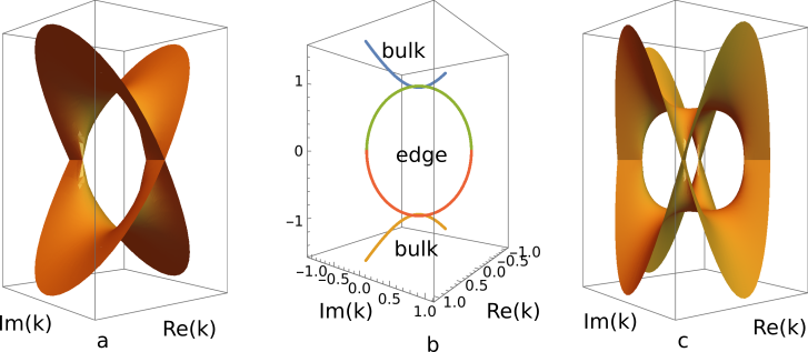
Starting point is the spectrum of the 2D Dirac Hamiltonian with real wave number and a positive Dirac mass . This example is considered for its simplicity but the concept can be directly generalized to other Hamiltonians with the bulk spectrum with an analytic function . The square root provides two bands for the 2D Dirac case, which are separated by a gap . Formally, this spectrum can be extended by continuing the real wave number to the complex plane. This creates a connected Riemann surface (cf. Fig. 1a,c). Therefore, the gap is bridged by modes with complex . However, a complex eigenvalue is not physical, such that we must restrict the analytic continuation to real values of . This is the case for real and for purely imaginary values with , where the latter gives . This means that the spectrum separates in a bulk spectrum with and and an edge spectrum with .
For the analytic continuation of the eigenfunctions we assume that the bulk mode is either a plane wave for a translational-invariant system or a circular wave with polar coordinates for a circular-invariant system. Then we obtain from the analytic continuations and either or , respectively. These modes decay exponentially for , , representing a so-called corner mode, or , representing a circular edge mode. The boundary conditions play obviously a crucial role here, since the edge modes should decay exponentially from the edge. This selects whether , are positive or negative. For a large disk with a central hole, for example, this means that at the edge of the hole.
We note that the analytic continuation does not affect the Hamiltonian, only the spectrum and the eigenfunctions. The analytic continuation can be reversed such that we get the bulk modes from the edge modes. This can be useful when we observe or manipulate the edge modes and want to determine the corresponding bulk modes.
4 Special examples
4.1 Single-band Laplacian model
We consider the eigenvalue problem with the Hamilton operator , acting on a 2D space, and the real energy eigenvalue . This equation appears in many areas of physics, for instance, in microwave systems, photonics and phononics. In the following, our models are characterized by different Hamiltonians . A prototype of is a single Laplacian on a disk with a non-negative bulk spectrum. For a the circular geometry is parametrized by polar coordinates as
| (8) |
The Bessel functions and are eigenfunctions of this Laplacian with eigenvalues [20]. Two linearly independent solutions are given by the linear combinations
| (9) |
with . The eigenvalues of are independent of due to the rotational invariance of the Laplacian.
The analytic continuation with a real yields negative eigenvalues and the modified Bessel functions as (cf. App. B)
| (10) |
where the modified Bessel function () increases (decreases) exponentially for and diverges for . A proper linear combination gives a unique solution that satisfies the boundary conditions at the edge. For a disk this is matched by with a finite value at and for a hole on a large disk it is matched by . The exponential decay rate of the edge modes is given by , indicating a radial shrinking of the edge modes with decreasing energy .
The requirement of the analytic continuation is that (i) the eigenvalues remain real and (ii) edge modes decay exponentially from an edge (i.e., they are evanescent modes). Thus, they depend strongly on the boundary conditions. We conclude that the spectrum of consists of two branches, which are parametrized by the complex wavenumber . One branch is for the bulk modes with and the other is for the edge modes with . Although both spectra are real, the bulk spectrum is parametrized by a real wavenumber, while the edge spectrum is parametrized by an imaginary wavenumber.
4.2 Two-band Laplacian model
The 2D Laplacian can be used to construct the Hamiltonian in Eq. (1) with , and . This yields the real symmetric matrix
| (11) |
Since the three-component vector is only a one-dimensional line in 2D, the bands have vanishing Chern numbers.
Now we consider a space with a circular geometry (e.g., a disk). Using the Laplacian in Eq. (8) and its eigenfunctions in Eq. (9), the ansatz
| (12) |
with the wavenumber yields
| (13) |
with the eigenvalues . The components of the eigenvectors read
| (14) |
with an additional normalization that depends on the specific physical system. The dependence of the eigenvalues suggests the analytic continuation with , such that is real. In Fig. 1c the analytic continuation of the bulk spectrum is depicted as a Riemann surface and compared with the Riemann surface of in Fig. 1a. It should be noted that this analytic continuation creates a non-Hermitian matrix in Eq. (13):
| (15) |
Their eigenvectors are not orthogonal, which implies that the edge modes are not orthogonal.
The analytic continuation of the eigenfunctions yields
| (16) |
These functions grow (decay) exponentially with . Boundary conditions select the unique solution. For instance, and are valid as an edge mode for a disk with radius , where the mode decays exponentially from the edge of the disk toward its center, and and are valid for a circular hole of radius in an infinite disk.
The two vector components , of the eigenfunctions in Eq. (12) do not depend on the polar angle . Thus, the field is uniform in space:
| (17) |
which describes a fixed semicircle on the unit sphere, beginning with at the North Pole, hitting at the equator and ending with at the South Pole. For the bulk modes are real such that for and for :
| (18) |
According to Eq. (14), on the other hand, for the edge modes is imaginary and is positive. This gives for two branches of edge modes with the phases , and
| (19) |
Thus, the bulk and the edge modes are associated with semicircles on the unit sphere, which meet the equator at or at , respectively. In both cases the EV vanishes due to , while the divergence of with respect to does not vanishes in the plane. Finally, the intensity as a function of the radius decays like for the bulk modes but is strongly localized at the edge for the edge mode.
4.3 Dirac model
Another example is a Dirac Hamiltonian , which reads with polar coordinates
| (20) |
It acts on a circular geometry and has the eigenfunctions (cf. App. A)
| (21) |
where can be expressed as the linear combination of Bessel functions of Eq. (9). , and are connected by two conditions (see Eq. (38) in App. A):
| (22) |
which implies and . The angular quantum numbers are , and the signs of and are fixed by the relations (22). Thus, the eigenvalues are degenerate with respect to , since is circular invariant. In other words, is the eigenvalue of the angular momentum operator, and the latter commutes with .
bulk modes in the upper band:
edge modes:
For and is imaginary and is real. On the other hand, for is real and is imaginary. In particular, for we have either , or , . This again is the analytic continuation for bulk to edge modes with , illustrated in Fig. 1b. Thus, from Eq. (9) we obtain edge modes with eigenvalues , which either grow or decay exponentially with on the scale for . This scale diverges as approach the spectral boundaries of the edge modes. On the other hand, the wavenumber of the bulk states vanishes as for . Therefore, are singular points in the spectrum, where the edge modes become uniformly extended over the entire 2D system. This is reminiscent of a localization-delocalization (or Anderson) transition in disordered systems and reflects the critical energy dependence of the edge modes and its transition to a bulk mode. These results suggest the introduction of an index in the wavefunction of Eq. (21)
| (23) |
where is either the band index for the upper and the lower band, or for the energies of the edge modes. This gives for the field
| (24) |
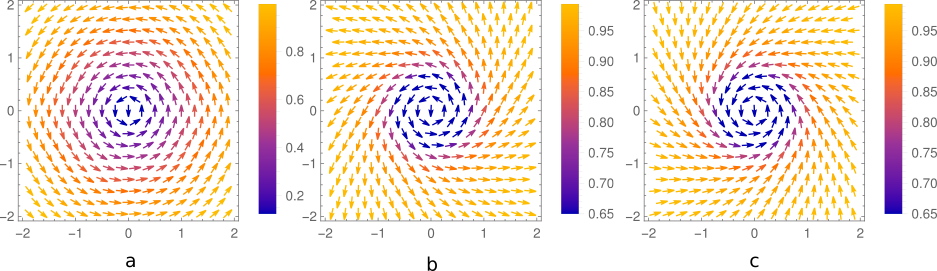
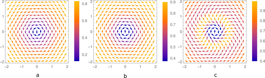
The projection is visualized for several eigenfunctions in Fig. 2. The phase shift is the angle between the radial vector and the projected vector . Comparing this expression with Eq. (4), we get the phase relation between the eigenfunctions and the field as
| (25) |
Besides the different energies for the bands and for the edge modes, also the parameter distinguishes the different modes. With the band energies we get from the relations in Eq. (22) for the bulk an imaginary parameter
| (26) |
On the other hand, for the edge modes we have a real parameter
| (27) |
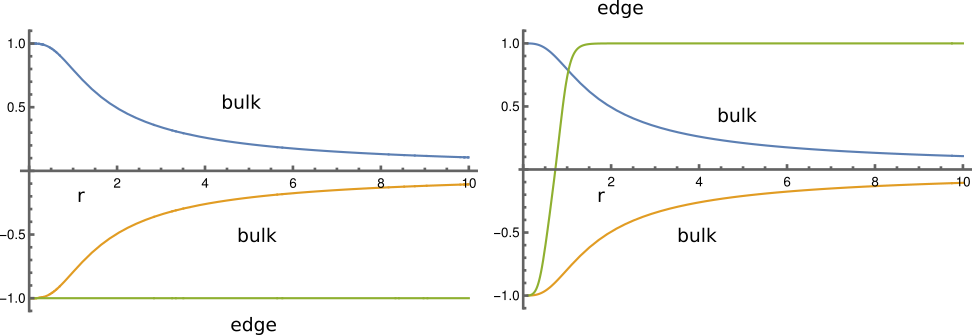
The behavior of the is presented in Fig. 4. can be understood as a topological number, analogous to the Chern number, which is associated with the band:
| (28) |
The phase shift in of Eq. (24) has different values for the two bands and for the edge modes due to . is plotted in Fig. 3 for bulk and edge modes and for different eigenfunctions.
There are transitions from bulk to edge modes at and from edge modes to bulk modes at . They are associated with a topological transition, indicated either by a change of or by a sign change of . The latter appears in the EV as
| (29) |
after an integration with respect to the edge of a circular hole with radius . EV is positive in the upper band and negative in the lower band (cf. Fig. 3). Since depends on the radius, the EV can change with the position of the edge.
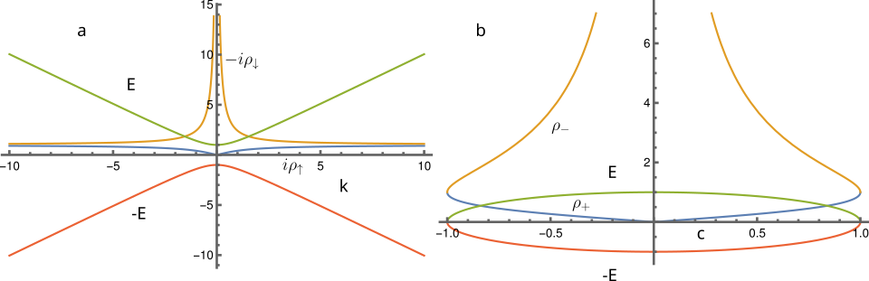
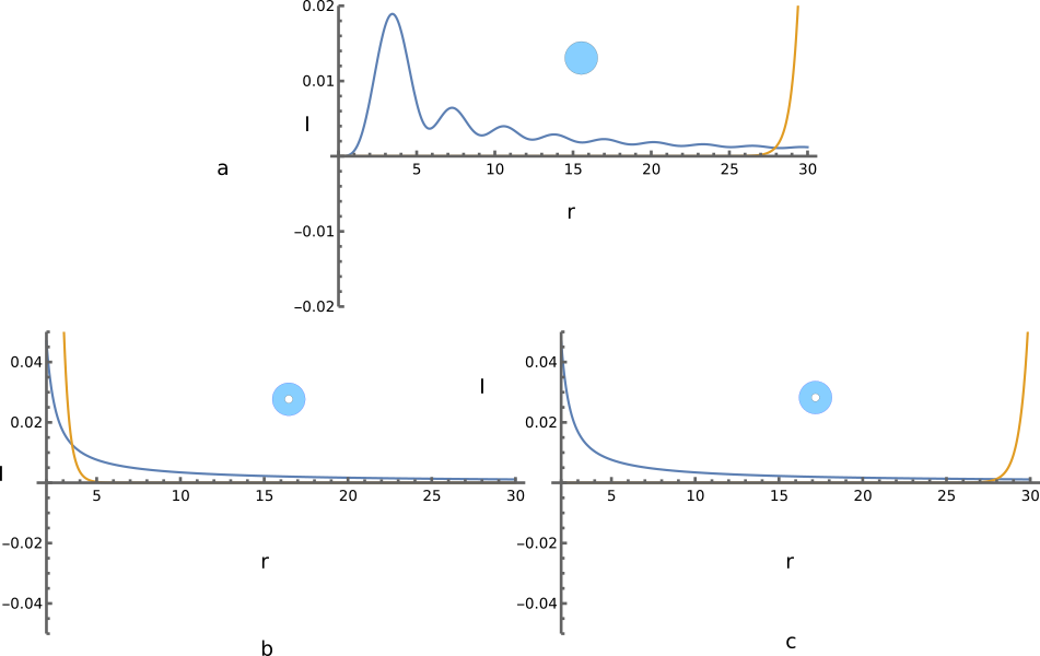
and diverge for , while and vanish in this limit (cf. Fig. 4), reflecting the change of the wavefunctions from edge-localized functions to circular waves at . At the critical point the vector reaches the South Pole. On the other hand, at the critical point the vector arrives at the North Pole. Finally, the intensity is plotted in Fig. 5 for different eigenfunctions. In all three cases the main difference is the significant weight of the edge mode intensity either at the center of the disk or at its boundary.
5 Discussion and conclusions
After having solved the eigenvalue equation for the bulk modes, the analytic continuation of the real wavenumber into the complex plane provides the edge modes. This approach yields a spectral separation of bulk and edge modes. On the other hand, there is no complete spatial separation of these two types of modes, since the edge modes extend into the bulk with an exponential decay on the scale :
| (30) |
This means that the edge modes are two-dimensional, which cannot be described as solutions of a one-dimensional equation. However, they do not spread over the entire system but decay exponentially from the edge. In contrast, the bulk modes decay like .
By varying we can scan continuously through the bulk and the edge spectrum. There are bulk-edge transitions at , representing transitions between localized edge modes and delocalized bulk modes. They are accompanied by topological transitions for the Dirac model, since the index and the sign of change according to Eq. (28) and Fig. 3. For the two-band Laplacian model the phase difference switches from for the upper band and for the lower band to for the two branches of the edge modes. This indicates that the bulk and the edge modes are not only characterized by their spatial decay but also by the phase difference in the field .
An important question concerns the robustness of the edge modes when we replace the uniform mass by a spatially varying mass . In the circular-symmetric case , a sign change of the mass creates an additional edge mode with a skyrmion-like wavefunction [16]. Moreover, with a positive we can break the circular symmetry. If , the robustness of the edge modes can be analyzed within perturbation theory. The (degenerate) perturbation expansion in powers of would provide a stability analysis of the edge modes. A thorough study of this perturbation approach exceeds the scope of this paper and should be left for a separate project in the future.
As a summary of the results of the two-band examples, we found the bulk eigenfunctions of circular symmetric two-band models. They are of the form
with real and complex. Physical properties are obtained from the field
The projection of the field identifies the phase difference of the two components of the eigenfunctions. An analytic continuation of yields the corresponding expressions for the edge modes. From these results we conclude that the BEC through an analytic continuation of the wavenumber offers a systematic approach for the description of two-band Hamiltonians with edges. Although we have focused here on a circular geometry for simplicity, the concept can be extended also to other geometries.
Appendix A Eigenfunctions of the Dirac Hamiltonian
With the ansatz
| (31) |
we can write for the eigenvalue problem the equation
| (32) |
which enables us to eliminate and , respectively, on both sides of the second equation:
| (33) |
Now we consider that is either the Bessel function , or a linear combination of these two functions and write and . Then we employ the recurrence relations of the Bessel functions [20]
| (34) |
and
| (35) |
With these relations we obtain from Eq. (33)
| (36) |
or the eigenvalue equation
| (37) |
which gives the relations
| (38) |
This determines the parameter in . Thus, we have and , both are independent of . The eigenfunction in Eq. (31) becomes
| (39) |
Appendix B Analytic continuation of Bessel functions
The analytic continuation with a real yields for the Bessel functions [20]
| (40) |
with , which implies
| (41) |
and
| (42) |
References
- [1] F. D. M. Haldane and S. Raghu. Possible realization of directional optical waveguides in photonic crystals with broken time-reversal symmetry. Phys. Rev. Lett., 100:013904, Jan 2008.
- [2] Ling Lu, John D. Joannopoulos, and Marin Soljačić. Topological photonics. Nature Photonics, 8(11):821–829, Nov 2014.
- [3] Tomoki Ozawa, Hannah M. Price, Alberto Amo, Nathan Goldman, Mohammad Hafezi, Ling Lu, Mikael C. Rechtsman, David Schuster, Jonathan Simon, Oded Zilberberg, and Iacopo Carusotto. Topological photonics. Rev. Mod. Phys., 91:015006, Mar 2019.
- [4] Xiang Ni, Simon Yves, Alex Krasnok, and Andrea Alù. Topological metamaterials. Chemical Reviews, 123(12):7585–7654, Jun 2023.
- [5] Gian Michele Graf and Marcello Porta. Bulk-edge correspondence for two-dimensional topological insulators. Communications in Mathematical Physics, 324(3):851–895, Dec 2013.
- [6] Pierre Delplace, J. B. Marston, and Antoine Venaille. Topological origin of equatorial waves. Science, 358(6366):1075–1077, 2017.
- [7] Gian Michele Graf and Clément Tauber. Bulk–edge correspondence for two-dimensional floquet topological insulators. Annales Henri Poincaré, 19(3):709–741, Mar 2018.
- [8] Bin Yan, Rudro R. Biswas, and Chris H. Greene. Bulk-edge correspondence in fractional quantum hall states. Phys. Rev. B, 99:035153, Jan 2019.
- [9] Kazuki Yokomizo and Shuichi Murakami. Non-bloch band theory and bulk–edge correspondence in non-hermitian systems. Progress of Theoretical and Experimental Physics, 2020(12):12A102, 09 2020.
- [10] Tianyu Li and Haiping Hu. Floquet non-abelian topological insulator and multifold bulk-edge correspondence. Nature Communications, 14(1):6418, Oct 2023.
- [11] Yohei Onuki, Antoine Venaille, and Pierre Delplace. Bulk-edge correspondence recovered in incompressible geophysical flows. Phys. Rev. Res., 6:033161, Aug 2024.
- [12] Gabriel Wong. A note on the bulk interpretation of the quantum extremal surface formula. Journal of High Energy Physics, 2024(4):24, Apr 2024.
- [13] Takuma Isobe, Tsuneya Yoshida, and Yasuhiro Hatsugai. Bulk-edge correspondence for nonlinear eigenvalue problems. Physical Review Letters, 132(12), March 2024.
- [14] K. S. Novoselov, A. K. Geim, S. V. Morozov, D. Jiang, M. I. Katsnelson, I. V. Grigorieva, S. V. Dubonos, and A. A. Firsov. Two-dimensional gas of massless dirac fermions in graphene. Nature, 438(7065):197–200, Nov 2005.
- [15] Xiaojun Cheng, Camille Jouvaud, Xiang Ni, S Hossein Mousavi, Azriel Z Genack, and Alexander B Khanikaev. Robust reconfigurable electromagnetic pathways within a photonic topological insulator. Nat Mater, 15(5):542–548, February 2016.
- [16] Klaus Ziegler. Circular edge states in photonic crystals with a dirac node. J. Opt. Soc. Am. B, 35(1):107–112, Jan 2018.
- [17] Jacob Shapiro. The bulk-edge correspondence in three simple cases. Reviews in Mathematical Physics, 32(03):2030003, 2020.
- [18] Roger S. K. Mong and Vasudha Shivamoggi. Edge states and the bulk-boundary correspondence in dirac hamiltonians. Phys. Rev. B, 83:125109, Mar 2011.
- [19] Klaus Ziegler and Roman Ya. Kezerashvili. Edge modes in chiral electron double layers, arxiv:2412.16760. 2024.
- [20] Milton Abramowitz and Irene A. Stegun. Handbook of Mathematical Functions with Formulas, Graphs, and Mathematical Tables. Dover Publications, Inc., New York, 1964.