HOPS: High-order Polynomials with Self-supervised Dimension Reduction for Load Forecasting

Abstract

Load forecasting is a fundamental task in smart grid. Many techniques have been applied to developing load forecasting models. Due to the challenges such as the Curse of Dimensionality, overfitting, and limited computing resources, multivariate higher-order polynomial models have received limited attention in load forecasting, despite their desirable mathematical foundations and optimization properties. In this paper, we propose low rank approximation and self-supervised dimension reduction to address the aforementioned issues. To further improve computational efficiency, we also introduce a fast Conjugate Gradient based algorithm for the proposed polynomial models. Based on the ISO New England dataset used in Global Energy Forecasting Competition 2017, the proposed method high-order polynomials with self-supervised dimension reduction (HOPS) demonstrates higher forecasting accuracy over several competitive models. Additionally, experimental results indicate that our approach alleviates redundant variable construction, achieving better forecasts with fewer input variables.

I Introduction

Electric load forecasting plays a crucial role in the contemporary energy industry. The accuracy of load forecasting models significantly affects various aspects of smart grid operations and planning, such as demand response, customer profiling, and upgrade of equipment. Many highly cited review articles can be found in the load forecasting literature [1, 2, 3, 4]. Various techniques have been proposed for load forecasting, such as multiple linear regression (MLR) [5, 6], artificial neural networks (ANN) [3, 7, 8], and support vector regression (SVR) [9, 10]. Three Global Energy Forecasting Competitions, including GEFCom2012 [11], GEFCom2014 [12] and GEFCom2017 [13], have stimulated the enthusiasm of the researchers across multiple disciplines, leading to further proposals of many effective methods. Several methods can been found from the reports of multiple winners of the three aforementioned load forecasting competitions, such as outlier detection and data cleaning prior to forecasting [5, 12], least absolute shrinkage and selection operator (LASSO)[14], forecast combination [15, 16, 17], and several machine learning techniques such as XGBoost and Gradient Boosting Machines [13, 18, 19].

From the perspective of model fitting, the models used by the contestants, even to the extend of the load forecasting community, can be roughly divided into two groups: statistical models, such as Multiple Linear Regression (MLR), and machine learning models, such has XGBoost and Artificial Neural Networks (ANN). There is no definitive distinction in forecasting accuracy between these two groups. Each has its own advantages and disadvantages. Statistical models are typically characterized by good interpretability, which allows researchers and practitioners to explain, refine, and defend their models. Machine learning models, on the other hand, tend to excel in fitting, which enables the forecasters to capture more intricate functional relationships between load and its driving factors.

Given these considerations, there is a clear motivation to identify a model that synthesizes the strengths of both approaches. Ideally, such a model should possess strong mathematical properties that facilitate improvements while offering superior fitting capabilities compared to traditional statistical models. In this regard, multivariate higher-order polynomials emerge as a promising candidate. However, despite the extensive use of sophisticated models in load forecasting competitions and related literature, the multivariate higher-order polynomial model has received comparatively little attention. A notable example is a family of interaction regression models with many third-order polynomial terms, which lead to hundreds of parameters to estimate for each model [20].

Arguably, polynomials are more frequently encountered in mathematics and statistics literature than in engineering-focused articles. We conjecture that there are three main reasons. The first one is The Curse of Dimensionality. The multivariate higher-order polynomial model inherently encounters the challenge of the Curse of Dimensionality, which results in excessively high computational complexity. For instance, when utilizing an $n$-dimensional $d$-order polynomial model for fitting, we require at least $\binom{d+n}{d}$ optimizable parameters to fully define the model. Even with sufficient computer memory to store these parameters, the time required to solve the model can be prohibitively long. In [10], the authors attempted to employ a quadric surface (an $n$-dimensional $2$-order polynomial model) to enhance the Support Vector Regression (SVR) model. However, due to the Curse of Dimensionality, they were forced to limit their analysis to only the diagonal elements of the quadratic term parameter matrix, which significantly diminished the model’s fitting capability compared to a fully parameterized polynomial model.

The second reason is overfitting. Although an increased number of parameters allows for a broader hypothesis space and more alternative functions for fitting training sets, it can also lead to severe overfitting. As the order of the polynomial rises, the number of parameters grows exponentially, making overfitting an inevitable consequence. As shown in [20], as more third-order polynomials of lag temperatures are added to the model, the forecast error decreases at first, and then increases when even more terms are added.

The third reason is limited computing power from both software and hardware. Load forecasting models based on high-order polynomials may include hundreds of parameters, which may require a long time for model selection and various tests. In addition, a large regression model may present numerical issues, so that many software packages may not be able to provide accurate estimation results. In fact, the primary reason the models proposed in [20] did not include temperatures of higher than the third order was due to the limitations in software and hardware at the time.

In light of these shortcomings, we aim to enhance the basic multivariate higher-order polynomial model to mitigate the impact of these issues while preserving the model’s overall effectiveness. Simultaneously, we also notice that in the models frequently utilized for load forecasting tasks [21, 1, 5, 6, 8, 22, 23, 20], researchers usually improve the forecasting accuracy by constructing complex interaction variables. Very often significant experience or expertise is required to select the appropriate combination of variables via a large number of empirical comparisons as done in [22]. Therefore, we also hope to utilize the multivariate higher-order polynomial models while eliminating the process of constructing complex interaction variables.

Our contributions can be summarized in the following three aspects. First, drawing on concepts of self-supervised dimension reduction and low-rank approximation, we introduce a dimension reduction approach for the high-order terms of the polynomial model. This method enables us to achieve superior forecasting accuracy while significantly reducing the number of required parameters. Secondly, we introduce a Conjugate Gradient-based (CG) optimization algorithm, which facilitates a more efficient and rapid solution to our improved polynomial model. Thirdly, our approach eliminates the need for complex interaction variable construction. Through numerical experiments, we demonstrate that our model can achieve superior performance compared to its counterparts even with fewer variables.

All numerical experiments are conducted on the ISO New England dataset. The results demonstrate that the proposed method high-order polynomials with self-supervised dimension reduction (HOPS) exhibits significant advantages over the benchmark and several competitive comparison models.

The remainder of this paper is organized as follows: Section II presents the fundamental methodology, including the mathematical formulation of the basic multivariate higher-order polynomial model and the self-supervised dimensionality reduction method. Related properties are also discussed in this section. Section III details the algorithm designed to accelerate computation for HOPS. Section IV outlines the experimental configuration, results, and analysis. Section V concludes our work and discusses potential future research directions. Finally, the Appendix includes proofs and statements related to the properties mentioned in Section II.

II Higher-order Polynomial Model and Self-supervised Dimension Reduction

II-A The Definition of $n$-dimensional $d$-order Polynomial

For an input feature vector $x_{1\times n}$ with $n$ input variables, the $n$-dimensional $d$-order polynomial $f$ is expressed as:

$$f\left(x_{1\times n},\boldsymbol{W_{0}},\boldsymbol{W_{1}},\cdots\boldsymbol{W_{d}}\right)=\textbf{sum}(\boldsymbol{W_{0}}*X_{0})$$

$$+\textbf{sum}(\boldsymbol{W_{1}}*X_{1})+\cdots,+\textbf{sum}(\boldsymbol{W_{d}}*X_{d}),$$ (1)

where $\textbf{sum}()$ denotes the point-by-point sum of tensors. $\boldsymbol{W_{i}}\in\mathbb{R}^{n^{i}}$ is a tensor of order $i$, representing the coefficient parameter tensor of $i$-order monomials. $X_{0}$ is a constant $1$ by default. The term $X_{i}=(x_{1\times n}\otimes x_{1\times n}\otimes\cdots\otimes x_{1\times n})$ represents the tensor product of the input vector repeated $i-1$ times. The mark $\ast$ denotes the Hadamard (element-wise) product and $\otimes$ denotes the tensor (outer) product. For better understanding, Fig. 1 provides visual representations of tensor products. A special case of the mathematical expression (II-A) where $\boldsymbol{deg}(f)=3$ is also shown in Fig. 2.

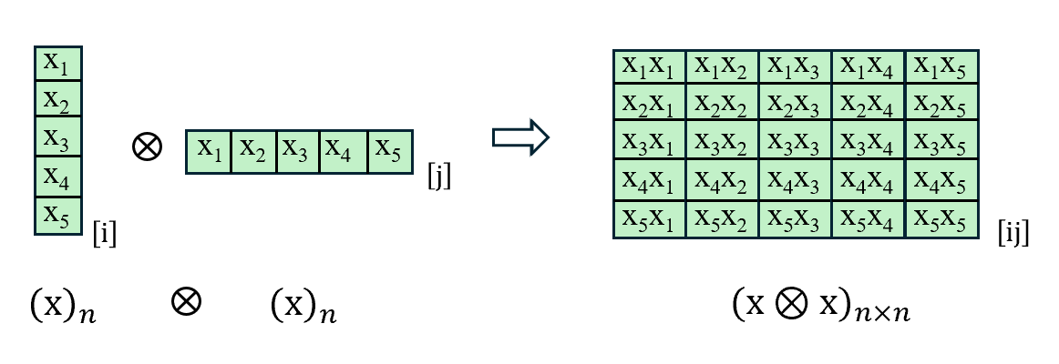
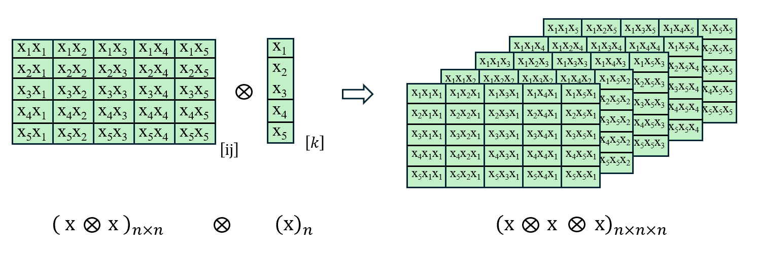
Figure 1: The tensor product of $x$ and $x$, $x\otimes x$ and $x$.

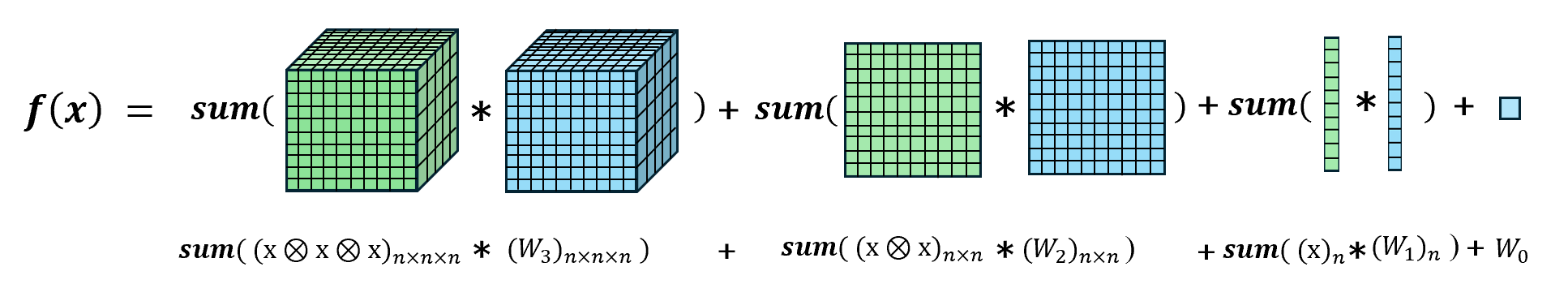
Figure 2: An $n$-dimensional $3$-order polynomial.

Similar to multiple linear regression (MLR), we fit the training samples by minimizing the squared error between the fitted values and the true values. Mathematically, this corresponds to solving the following optimization problem:

$$\min_{\boldsymbol{W_{0}}\in\mathbb{R}^{1},\cdots,\boldsymbol{W_{d}}\in\mathbb{R}^{n^{d}}}\sum_{p=1}^{m}(f\left((x_{1\times n})_{p},\boldsymbol{W_{0}},\cdots\boldsymbol{W_{d}}\right)-\boldsymbol{y}_{p})^{2},$$ (2)

where $(x_{1\times n})_{p}$ and $\boldsymbol{y}_{p}$ are the input feature vector and the label corresponding to $p$-th sample, respectively. There are $m$ samples for training in total. The goal is to find the optimal parameter tensors $\{\boldsymbol{W_{i}},i=0,1,2,\cdots,d\}$. To regularize the model and prevent overfitting, we can introduce $L_{2}$ regularization $\sum_{i=0}^{d}\lambda_{i}||\boldsymbol{W_{i}}||^{2}_{F}$ to penalize large parameters, where $\lambda_{i}$ controls the strength of regularization for the parameter tensor $\boldsymbol{W}_{i}$, and $\|\cdot\|_{F}$ represents the Frobenius norm. For simplicity, we will not include $\sum_{i=0}^{d}\lambda_{i}||\boldsymbol{W_{i}}||^{2}_{F}$ in the following numerical experiments. However, differentiated regularization through $\lambda_{i}$ may play an important role in improving resistance to overfitting.

II-B Self-supervised Dimension Reduction

In this subsection, we introduce our dimension reduction method aimed at addressing the Curse of Dimensionality.

Our approach relies on finding a low-rank linear transformation matrix $T_{n\times n}$ to reduce the requirement for the number of parameters while preserving the essential information of the data. Specifically, we solve the following optimization problem:

$$\min_{T_{n\times n}\in\mathbb{R}^{n\times n}}Loss(X_{m\times n}\cdot T_{n\times n},X_{m\times n}),$$ (3)

$$s.t.\quad\textbf{{rank}}(T_{n\times n})=k,k<n,$$

where $X_{m\times n}$ denotes the matrix obtained by arranging $m$ sample feature vectors $x_{1\times n}$ in rows. The loss function measures the distance between the low-rank approximation of the input feature matrix and the original matrix. Utilizing the Frobenius norm, we express the loss as $Loss=\left\lVert X_{m\times n}\cdot T_{n\times n}-X_{m\times n}\right\rVert_{F}^{2}$. Without loss of generality, we suppose that $\textbf{rank}(X_{m\times n})=r>k$. By decomposing $T_{n\times n}$ into $L_{n\times k}\cdot R_{k\times n}$, we can effectively reduce the dimensionality of the input data while preserving important information for forecasting. The reduced data, denoted as $\tilde{X}_{m\times k}$, is obtained by applying the linear transformation matrix $L_{n\times k}$ to the original data:

$$\tilde{X}_{m\times k}=X_{m\times n}\cdot L_{n\times k}.$$

This dimension reduction provides three main benefits:

1. Reduce Computational Complexity: Taking $d$-order terms as an example, when we denote the input feature matrix as $\widetilde{X}_{m\times k}$ (a single input sample feature vector is denoted as $\widetilde{x}_{1\times k}$), the $d$-order term sums to $\textbf{sum}((\boldsymbol{W_{d}})_{k\times k\cdots k}*\widetilde{X}_{d})=\textbf{sum}((\boldsymbol{W_{d}})_{k\times k\cdots k}*(\widetilde{x}_{1\times k}\otimes\widetilde{x}_{1\times k}\otimes\ldots\otimes\widetilde{x}_{1\times k}))$ , where the number of parameters to optimize in the $d$-order parameter tensor $\boldsymbol{W_{d}}$ is reduced from $\mathcal{O}(n^{d})$ to $\mathcal{O}(k^{d})$.

2. Preserve Model Fitting Capacity: The model maintains its ability to capture complex relationships, as the dimension reduction is applied in a way that preserves the core structure of the input features. For illustration, consider the quadratic term:

   $$\textbf{sum}\left((\boldsymbol{W_{2}})_{n\times n}*((x_{1\times n}\cdot T_{n\times n})\otimes(x_{1\times n}\cdot T_{n\times n}))\right)$$

   $$= (x_{1\times n}\cdot T_{n\times n})\cdot(\boldsymbol{W_{2}})_{n\times n}\cdot(T_{n\times n}^{T}\cdot x_{1\times n}^{T})$$

   $$= (x_{1\times n}\cdot L_{n\times k})\cdot\underbrace{R_{k\times n}\cdot(\boldsymbol{W_{2}})_{n\times n}\cdot R_{k\times n}^{T}}_{(\boldsymbol{W_{2}^{\prime}})_{k\times k}}\cdot(L_{n\times k}^{T}\cdot x_{1\times n}^{T})$$

   $$= \widetilde{x}_{1\times k}\cdot(\boldsymbol{W_{2}^{\prime}})_{k\times k}\cdot\widetilde{x}_{1\times k}^{T}$$

   $$= \textbf{sum}((\boldsymbol{W_{2}^{\prime}})_{k\times k}*(\widetilde{x}_{1\times k}\otimes\widetilde{x}_{1\times k}))$$

   where $(\boldsymbol{W_{2}^{\prime}})_{k\times k}$ and $(\boldsymbol{W_{2}})_{n\times n}$ denote $k$-dimensional $2$-order and $n$-dimensional $2$-order optimizable parametric tensors (or matrices) respectively. For any $(\boldsymbol{W_{2}})_{n\times n}$, there exists a corresponding $(\boldsymbol{W_{2}^{\prime}})_{k\times k}=R_{k\times n}\cdot(\boldsymbol{W_{2}})_{n\times n}\cdot R_{k\times n}^{T}$ such that the above relationship holds for any $x_{1\times n}\in\mathbb{R}^{n}$. This demonstrates that optimizing the polynomial model with $\widetilde{X}_{m\times k}$ as the input feature matrix is equivalent to obtaining a low-rank approximation of $X_{m\times n}$ (i.e. $X_{m\times n}\cdot T_{n\times n}$) and then feeding it into the full-parameter polynomial model for optimization. When the polynomial order exceeds two, a similar process can be followed using tensor notation.

3. Overfitting Regularization: After the embedding through the matrix $L_{n\times k}$, the number of parameters that can be freely adjusted in the model has been significantly reduced. Appropriate $k$ can decrease the risk of overfitting.

Additionally, we can apply different $k_{i}$ for different terms. As the order $i$ increases, the number of parameters in $\boldsymbol{W_{i}}$ increases exponentially. We can therefore choose a smaller $k_{i}$ when $i$ is larger to keep the computation manageable. It is also important to emphasize that when obtaining the matrix $L_{n\times k}$, we can only use training set data and must not rely on future input features to avoid data leakage.

For convenience we denote the $i$-order optimizable parameter tensor $(\boldsymbol{W_{i}})_{k_{i}\times k_{i}\cdots\times k_{i}}$ as $(\boldsymbol{W_{i}})_{k_{i}}$ and denote $\underbrace{\widetilde{x}_{1\times k_{i}}\otimes\widetilde{x}_{1\times k_{i}}\cdots\otimes\widetilde{x}_{1\times k_{i}}}_{i}=(x_{1\times n}\cdot L_{n\times k_{i}})\otimes(x_{1\times n}\cdot L_{n\times k_{i}})\otimes\cdots(x_{1\times n}\cdot L_{n\times k_{i}})$ as $\widetilde{X_{i}}$ $(i=1,2,\cdots d)$. So our model after dimension reduction embedding can be represented as:

$$\widetilde{f}\left(x_{1\times n},\boldsymbol{W_{0}},(\boldsymbol{W_{1}})_{k_{1}},\cdots,(\boldsymbol{W_{d}})_{k_{d}}\right)$$

$$= \boldsymbol{W_{0}}+\textbf{sum}\left((\boldsymbol{W_{1}})_{k_{1}}*\widetilde{X_{1}}\right)+\cdots\textbf{sum}\left((\boldsymbol{W_{d}})_{k_{d}}*\widetilde{X_{d}}\right),$$ (4)

and the optimization problem can be expressed as:

$$\min_{(\boldsymbol{W_{i}})_{k_{i}}\in\mathbb{R}^{(k_{i})^{i}}}\sum_{p=1}^{m}(\widetilde{f}-\boldsymbol{y}_{p})^{2}.$$ (5)

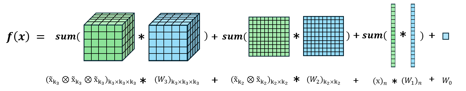
Figure 3: An $n$-dimensional $3$-order polynomial with quadratic term embedding dimension $k_{2}$ and cubic term embedding dimension $k_{3}$.

In practice, we can obtain suitable $k_{i}(i=1,2,\cdots)$ by a validation set or directly specify fixed $k_{i}$ based on experience. For load forecasting tasks, the polynimoal model’s performance is not highly sensitive to the choice of $k_{i}$, allowing us to make reasonable adjustments based on computational cost. Thus, we have presented the complete polynomial model. Since the model is based on high-order polynomials with self-supervised dimensionality reduction, we refer to it as HOPS. We provide an illustration in Fig. 3.

It is worth noting that if Z-score normalization is applied to the input data, the dimension reduction process described above becomes nearly equivalent to PCA in mathematical terms. In the case of load forecasting, the input variables are mostly categorical variables, so we generally do not use Z-score normalization.

II-C Properties and the Analytical Solution

In this subsection, we provide some useful properties.

First, we highlight that the optimal solution to Problem (5) exists, and the optimal solution set is either a single value or an affine space of $\mathbb{R}^{\sum_{i=0}^{d}(k_{i})^{i}}$. This is due to the fact that Problem (5) can be reformulated as a large-scale linear regression problem. The specific details are provided in Theorem 3 of Appendix II.

Second, with regard to the optimization problem (3), when the Frobenius norm is used as the loss function, an analytical solution can be derived by applying Singular Value Decomposition (SVD) and the Eckart-Young-Mirsky Theorem. In particular, the solution requires performing Singular Value Decomposition on the input feature matrix $X_{m\times n}$, allowing us to decompose $X_{m\times n}$ in the following manner:

$$X_{m\times n}=U_{m\times m}\Sigma_{m\times n}V_{n\times n}^{T}.$$

Next, we take the first $k$ columns of $V_{n\times n}$ to obtain the required matrix $L_{n\times k}$. A detailed explanation of this process is provided in Theorem 2 of Appendix I.

Additionally, there is an important point to consider here. Even though $T_{n\times n}$ is unique, $L_{n\times k}$ is not necessarily unique. Any $L_{n\times k}$ can be transformed into a new matrix $L_{n\times k}^{\prime}$ through an invertible linear transformation. This raises a natural concern: will the forecasting results change if we apply a different $L_{n\times k}$ for embedding? Fortunately, we can prove that any $L_{n\times k}$ that satisfy the condition $T_{n\times n}=L_{n\times k}R_{k\times n}$, will be equivalent to our model. A detailed statement of this conclusion and its proof can be found in Theorem 4 of Appendix III.

III A Fast Algorithm for Multivariate Higher-order Polynomial Model

III-A Algorithm Overview

In this section, we mainly describe the details about the fast algorithm applied to the embedded $n$-dimensional $d$-order polynomial model proposed in the previous section.

While we have already reduced the memory requirement from $\mathcal{O}(n^{d})$ to $\mathcal{O}(k^{d})$ by dimension reduction, the computational complexity still grows exponentially with $d$. Even with a relatively small $k$, the computational burden can remain significant. Fortunately, the inherent mathematical structure of the polynomial model provides a way to address this challenge. By leveraging the tensor representation of $n$-dimensional $d$-order polynomials, we introduce a fast algorithm, as outlined in Algorithm 1, to efficiently solve the Fitting Problem (5). We name it as PolyCG (a modified FR-CG method for the polynomial model).

For simplicity, in this subsection we denote $\widetilde{f}^{j}\left(\boldsymbol{x}\right)$ and $\widetilde{f}^{j}_{\boldsymbol{R}}\left(\boldsymbol{x}\right)$ as a shorthand for $\widetilde{f}\left(\boldsymbol{x},\boldsymbol{W_{0}}^{j},(\boldsymbol{W_{1}})_{k_{1}}^{j},\cdots,(\boldsymbol{W_{d}})_{k_{d}}^{j}\right)$ and $\widetilde{f}\left(\boldsymbol{x},\boldsymbol{R}_{0}^{j},\boldsymbol{R}_{1}^{j},\cdots,\boldsymbol{R}_{d}^{j}\right)$ respectively. We also represent $(\underbrace{x_{1\times n}L_{n\times k_{i}}\otimes x_{1\times n}L_{n\times k_{i}}\otimes\cdots x_{1\times n}L_{n\times k_{i}}}_{i})$ as $\widetilde{X}_{i}(x)$. The superscript $j$ in the context all represents the $j$-th iteration. Additionally, $\alpha^{j}$ is computed as follows:

$$\alpha^{j}=\frac{\sum_{i=0}^{d}\left\|\boldsymbol{R}_{i}^{j}\right\|_{F}^{2}}{2\left(\sum_{p=1}^{m}(\widetilde{f}^{j}_{\boldsymbol{R}}\left(\boldsymbol{x}_{p}\right)-\boldsymbol{0})^{2}\right)},$$ (6)

and $\boldsymbol{R}_{i}^{j}$ is computed by:

$$\boldsymbol{R}_{i}^{j} =\frac{\partial\left(\sum_{p=1}^{m}(\widetilde{f}^{j}\left(\boldsymbol{x}_{p}\right)-\boldsymbol{y}_{p})^{2}\right)}{\partial(\boldsymbol{W}_{i})^{j}_{k_{i}}} =\sum_{p=1}^{m}2(\widetilde{f}^{j}\left(\boldsymbol{x}_{p}\right)-\boldsymbol{y}_{p})\widetilde{X}_{i}(\boldsymbol{x}_{p}).$$ (7)

Owing to the favorable mathematical properties of $n$-dimensional $d$-order polynomials and the tensor-based formulation defined in equation (II-A), any derivative process can be analytically expressed as a simple combination of additions and multiplications between tensors or tensors and scalars. Similar to the optimization advantages observed in deep neural networks, this characteristic is well-suited for GPU parallel computing, as GPUs excel at performing simple but large-scale matrix and tensor operations. Consequently, these numerical computations can be efficiently handled by PyTorch, Nvidia GPUs, and CUDA with minimal effort.

Algorithm 1 PolyCG

0: Training Feature Set $\boldsymbol{X}$; Training Label Set $\boldsymbol{Y}$; Initial Values of the Parameter Tensors $(\boldsymbol{W}_{i})_{k_{i}}^{0},i=0,1,2,\cdots d$; Embedding Dimensions For Different Order Terms $\{k_{i},i=1.2,\cdots d\}$; Maximum Iteration $K=1000$; the Tolerance $\epsilon=1e-7$.

0: Values of the parameter tensors $(\boldsymbol{W}_{i})_{k_{i}}^{j},i=0,1,2,\cdots d$;

1: Calculate $\boldsymbol{R}^{0}_{i},i=0,1,2,\cdots d$;

2: Let $\boldsymbol{P}^{0}_{i}=-\boldsymbol{R}^{0}_{i},i=0,1,2,\cdots d$;

3: for $j=0$ to $K-1$ do

4:  Calculate $\alpha^{j}$;

5:  $(\boldsymbol{W}_{i})_{k_{i}}^{j+1}=(\boldsymbol{W}_{i})_{k_{i}}^{j}+\alpha^{j}\boldsymbol{P}^{j}_{i},i=0,1,2,\cdots d$;

6:  Obtain $\widetilde{f}^{j+1}$ by $(\boldsymbol{W}_{i})_{k_{i}}^{j+1},i=0,1,2,\cdots d$;

7:  If $\frac{|\sum_{p=1}^{m}(\widetilde{f}^{j+1}\left(\boldsymbol{x}_{p}\right)-\boldsymbol{y}_{p})^{2}-\sum_{p=1}^{m}(\widetilde{f}^{j}\left(\boldsymbol{x}_{p}\right)-\boldsymbol{y}_{p})^{2}|}{\sum_{p=1}^{m}(\widetilde{f}^{j}\left(\boldsymbol{x}_{p}\right)-\boldsymbol{y}_{p})^{2}}\leq\epsilon$, terminate the loop.

8:  Calculate $\boldsymbol{R}_{i}^{j+1},i=0,1,2,\cdots d$;

9:  $\beta^{j}=\frac{\sum_{i=0}^{d}\left\|\boldsymbol{R}_{i}^{j+1}\right\|_{F}^{2}}{\sum_{i=0}^{d}\left\|\boldsymbol{R}_{i}^{j}\right\|_{F}^{2}}$;

10:  Calculate $\boldsymbol{P}_{i}^{j+1}=-\boldsymbol{R}_{i}^{j+1}+\beta^{j}\boldsymbol{P}_{i}^{j},i=0,1,2,\cdots d$;

11: end for

12: Return Values of the parameter tensors $(\boldsymbol{W}_{i})_{k_{i}}^{j},i=0,1,2,\cdots d$.

III-B A Note on Algorithm 1

Essentially, the solution of the proposed model can be interpreted as a large-scale linear regression problem. This provides a simple and intuitive way to conceptualize the polynomial model. By extending the feature space geometrically, the model can fit the dataset in a much higher-dimensional space. However, this approach is often computationally impractical. Super-high-dimensional linear regression typically involves the inversion and multiplication of extremely large matrices, which are both computationally expensive and memory-intensive, especially when $\sum_{i=0}^{d}(k_{i})^{i}$ is too large. Given the necessity to solve large-scale linear equations or optimization problems under limited computational and storage resources, the CG method presents itself as a viable solution [24]. This method has been well-studied and proven effective in such contexts [25]. Therefore, building on the core principles of CG, we modify the Fletche Reeves CG algorithm (FR-CG) [26] to provide a practical and efficient approach, as presented in Algorithm 1, specifically adapted to solve the optimization problem (5). It is worth noting that in practice, the number of iterations required is often significantly less than $\sum_{i=0}^{d}(k_{i})^{i}$, which is required for an exact solution theoretically. Due to round-off error, when the problem scale is too large, the algorithm only obtains an approximate numerical solution.

IV Numerical Experiment

IV-A Datasets and Metrics

IV-A1 Datasets

The dataset utilized for our numerical experiments is the ISO New England (ISONE) dataset, which was used in Global Energy Forecasting Competition 2017. This dataset is chosen due to the extensive body of research conducted on it, facilitating easier comparisons with existing methods. This dataset consists of 10 hourly load datasets from the ISO New England, covering eight load zones: Maine (ME), New Hampshire (NH), Vermont (VT), Connecticut (CT), Rhode Island (RI), Southeastern Massachusetts (SEMASS), Western Central Massachusetts (WCMASS), and Northeastern Massachusetts (NEMASS). Additionally, it includes the combined load for the three Massachusetts regions (MASS) and the total combined load for all regions (TOTAL). The dataset also provides hourly drybulb temperature and dew point temperature data. Relative humidity can be calculated from drybulb temperature and dew point temperature by the Tetens equation. We pick three years (2012-2014) of hourly data for training and one year (2015) for testing.

IV-A2 Evaluation Metrics

Although various evaluation metrics are employed for load forecasting, Mean Absolute Percentage Error (MAPE) is most commonly used due to its transparency and simplicity [6, 10, 22]. The MAPE is defined as:

$$MAPE=\frac{1}{N}\sum_{t=1}^{N}\left|\frac{y_{t}-\widehat{y_{t}}}{y_{t}}\right|\times 100\%,$$

where $y_{t}$ and $\widehat{y_{t}}$ are the actual load and the predicted load at time $t$, respectively. $N$ denotes the number of samples.

To diversify the evaluation metrics, we also utilize another widely adopted metric, Mean Squared Error (MSE), which is also commonly used in load forecasting studies, such as in [10]. The MSE is defined as:

$$\text{MSE}=\frac{1}{N}\sum_{t=1}^{N}\left({y_{t}-\widehat{y_{t}}}\right)^{2},$$

where $y_{t}$, $\widehat{y_{t}}$ and $N$ are the same as above.

IV-B Implementation Details

All numerical experiments are conducted on a desktop equipped with a 12th Gen Intel(R) i5-12600KF CPU, 32.0 GB usable RAM, H800 GPU with 80GB RAM and Microsoft Windows 11 Enterprise. We implement our algorithm through Python 3.11.5, CUDA 12.6 and Jupyter Notebook 6.5.4.

For hyperparameter settings, we set the maximum number of iterations to be 1000 and the tolerance $\epsilon=1e-7$. Similar to [10], we normalize all input variables by Min-Max normalization. Since the primary term is generally less prone to overfitting, we set $k_{1}$ equal to the sample feature dimension $n$. Given the relatively straightforward relationship between load and features, we limit the max polynomial order $d=3$, rather than opting for a larger order. The optimal embedding dimensions $k_{2}$ and $k_{3}$ are chosen by a validation set (the data of 2014). We retrain the model on the whole training set (2012-2014) after getting $k_{2}$ and $k_{3}$ on the validation set.

The trend item $Trend_{t}$ is not treated as a typical feature variable. Given its particular nature, we include it in the primary term but exclude it from the higher-order terms and then remove it before performing dimension reduction. So the highest optional embedding dimension for the higher-order terms is set to be $n-1$ ($1$ less than the input feature dimension). When we perform a grid search to select the optimal embedding dimensions $k_{2}$ and $k_{3}$, we set the quadratic term embedding dimension range to be $[12,24,36,48,60,72,84,96,108]$ and the cubic term embedding dimension range to be $[0,1,5,9,13,17,21]$ for data with a feature dimension of 289. For other input data, we set the quadratic term embedding dimension range to be $[20,28,36,44,52,60,68,76,84]$ (if greater than $n-1$, replace it with $n-1$) and the cubic term embedding dimension range to be $[0,1,5,9,13,17,21]$. For practicality, when using a variable selection method similar to the Recency model, we fix $k_{2}=60$ and $k_{3}=9$.

IV-C The Competitive Benchmark

Hundreds of models have been developed for load forecasting [23]. However, as noted in [6, 10], one of the most frequently cited is constructed in the following manner:

$$y_{t}= r_{0}+r_{1}Trend_{t}+r_{2}H_{t}+r_{3}W_{t}+r_{4}M_{t}$$

$$+r_{5}H_{t}W_{t}+f(T_{t}),$$

where $y_{t}$ denotes the load value that needs to be predicted at time $t$, $H_{t}$ is dummy variables (a vector) corresponding to 24 hours per day. $W_{t}$ is dummy variables (a vector) indicating seven days of a week. $M_{t}$ is dummy variables (a vector) indicating 12 months of a year. $T_{t}$ denotes the concurrent temperature. $Trend_{t}$ is a variable of the increasing integers representing a linear trend and

$$f\left(T\right)= \beta_{1}T+\beta_{2}\left(T\right)^{2}+\beta_{3}\left(T\right)^{3}+\beta_{4}T_{t}H_{t}+\beta_{5}\left(T\right)^{2}H_{t}+$$

$$\beta_{6}\left(T\right)^{3}+\beta_{7}TM_{t}+\beta_{8}\left(T\right)^{2}M_{t}+\beta_{9}\left(T\right)^{3}M_{t}.$$

In [10], the authors did not include $\left(T_{t}\right)^{k}$ as variables in their regression model to avoid perfect multicollinearity. Similarly, $H_{t}$ and $W_{t}$ were excluded for the same reason. Following the approach outlined in [10], we combine the variables to obtain 289-dimensional input variables for MLR. As a widely recognized and effective method for load forecasting, this feature-based MLR model has been frequently cited and utilized as a benchmark in GEFCom2012, GEFCom2014, and GEFCom2017. We refer to this vanilla model as $G_{1}$.

In [8], the authors highlighted the significant role of humidity in load forecasting and recommended a model as follows:

$$y_{t}=g(RH_{t})+G,$$

where $G$ represents a base model depending upon temperature variables, and

$$g(RH_{t})= \gamma_{1}RHS_{t}+\gamma_{2}RHS_{t}^{2}+\gamma_{3}T_{t}\times RHS_{t}+\gamma_{4}T_{t}^{2}\times RHS_{t}$$

$$+\gamma_{5}T_{t}\times RHS_{t}^{2}+\gamma_{6}T_{t}^{2}\times RHS_{t}^{2}+\gamma_{7}H_{t}\times RHS_{t}$$

$$+\gamma_{8}H_{t}\times RHS_{t}^{2}.$$

$H_{t}$ and $T_{t}$ are the same as before. $RH$ denotes relative humidity (%). $S_{t}$ denotes a dummy variable indicating Jun.-Sep. of a year. $RHS_{t}$ denotes cross effect of relative humidity and summer. $RHS_{t}^{2}$ denotes cross effect of relative humidity square and summer. All the above symbols are consistent with [8]. We take $G=G_{1}$ and denote $y_{t}=g(RH_{t})+G_{1}$ as $H_{1}$.

Additionally, following the approach in [20], we incorporate lagged temperature variables and obtain an improved model that only depends on the temperature and date:

$$y_{t}= r_{0}+r_{1}Trend_{t}+r_{2}H_{t}+r_{3}W_{t}+r_{4}M_{t}$$

$$+r_{5}H_{t}W_{t}+\sum_{h=0}^{3}f(T_{t-h}),$$

where $H_{t},W_{t},M_{t}$ are the same as above. $T_{t-h}$ denotes the temperature of the previous $h$-th hour. As before, $\left(T_{t-h}\right)^{k}$, $H_{t}$ and $W_{t}$ are excluded to avoid perfect multicollinearity. This results in a total of 613 variables and we refer to it as $G_{2}$. By incorporating both humidity information and lagged temperature variables, we present this second improved model for comparison:

$$y_{t}=g(RH_{t})+G_{2}.$$

We denote this model as $H_{2}$.

In conclusion, these two improved models, $H_{1}$ and $H_{2}$, contain $343$ and $667$ variables, respectively.

IV-D Overall Performance with the Same or Simpler Inputs

First, to demonstrate that the improved performance of our proposed method is due to the method itself rather than changes in variables, we utilize the same variables from the vanilla model $G_{1}$ as the underlying variables for our proposed model, which is named as HOPS289 (the HOPS Model with 289 variables) for distinction. The experimental results are presented in Table I. It is evident that our model outperforms the vanilla model $G_{1}$ in terms of load forecasting accuracy across all regions, regardless of whether MAPE or MSE is used as the evaluation metric.

In [6, 10], the authors selected and constructed 289 variables based on their practical significance to get the vanilla model $G_{1}$, whose high accuracy is largely attributed to the complexity of the variable construction process. However, this process can be somewhat tedious. Our goal is to achieve better prediction performance with simpler input variables, which will be more beneficial for including more relevant variables and solving the model. Fortunately, we have found that our model can achieve comparable forecasting performance without the necessity for such intricate variable construction.

Specifically, rather than constructing interaction terms, we utilize the same underlying input information (temperature and date) but with fewer variables compared to the vanilla model $G_{1}$. The selected input variables are $\{Trend_{t}$, $H_{t}$, $W_{t}$, $M_{t}$, $T_{t}$, $(T_{t})^{2}$, $(T_{t})^{3}\}$, 47 variables in total. We refer to this model as HOPS47. To assess the impact of complex versus simple input variables on our model’s performance, we compare the forecasting results utilizing $47$-dimensional input variables against those utilizing $289$-dimensional input variables. The experimental results and the comparison are also presented in Table I.

The experimental results indicate that the two sets of input variables make little difference in our model’s performance. The accuracy of both HOPS47 and HOPS289 is nearly identical, and both outperform the vanilla model $G_{1}$. Although, on average, HOPS289 performs slightly better than HOPS47, the variable construction of HOPS47 is simpler and easier. Moreover, the computation time for HOPS47 is significantly lower than that of HOPS289, as HOPS289 typically requires a broader search range for the embedding dimension $k_{2}$ and $k_{3}$, which means that it will take us more time to train the model. It takes 19 minutes 24 seconds to finish all the numerical experiments for HOPS47 while 66 minutes 9 seconds for HOPS289. We recommend using the variable input method of HOPS47.

TABLE I: Comparisons Between $G_{1}$ and HOPS289, HOPS47.

	MAPE(%)			MSE (×103)
	HOPS		$G_{1}$	HOPS		$G_{1}$
Zone	289dim	47dim		289dim	47dim
CT	3.99	4.03	4.18	38.68	38.76	42.52
MASS	3.60	3.64	3.81	109.80	110.51	122.42
ME	4.38	4.38	4.50	4.96	4.98	5.25
NEMASS	3.66	3.66	3.90	25.36	25.48	28.53
NH	3.52	3.48	3.73	4.21	4.12	4.75
RI	3.64	3.72	3.86	2.40	2.46	2.78
SEMASS	4.31	4.40	4.64	10.41	10.78	11.98
VT	4.08	4.08	4.29	1.21	1.18	1.29
WCMASS	4.28	4.30	4.41	13.04	12.86	13.78
AVERAGE	3.94	3.97	4.15	23.34	23.46	25.92
TOTAL	3.37	3.41	3.54	454.62	457.13	501.55

IV-E Overall Performance with Other Advanced Models

Currently, many load forecasting models primarily improve forecasting accuracy by selecting more relevant variables, such as incorporating humidity information [8] or leveraging recency effects [20]. However, these models merely increase the input variables without considering improving performance by altering the model’s fitting function. Below, we compare the advantages of our model over these advanced models under the same input information.

Similar to HOPS47, we do not construct interaction terms and use the same temperature, relative humidity, and date information as in $H_{1}$ and $H_{2}$. Specifically, for $H_{1}$, the variables include { $Trend_{t}$, $H_{t}$, $W_{t}$, $M_{t}$, $T_{t}$, $(T_{t})^{2}$, $(T_{t})^{3}$, $RH_{t}$, $(RH_{t})^{2}$, $(RH_{t})^{3}$ }, resulting in a total of 50 variables. For $H_{2}$, the variables include {$Trend_{t}$, $H_{t}$, $W_{t}$, $M_{t}$, $T_{t}$, $(T_{t})^{2}$, $(T_{t})^{3}$, $RH_{t}$, $(RH_{t})^{2}$ $(RH_{t})^{3}$, $T_{t-i}$, $(T_{t-i})^{2}$, $(T_{t-i})^{3}$, $i=1,2,3$ }, totaling 59 variables. We refer to these models as HOPS50 and HOPS59, respectively. $H_{1}$ and HOPS50 share the same input information, although there are different input variables for these two models. The relationships between $G_{1}$ and HOPS47, $H_{2}$ and HOPS59 are similar to $H_{1}$ and HOPS50. The experimental results and the comparison are presented in Table II. It can be observed that our model consistently demonstrates a stable advantage when the input information is the same. Moreover, as the input information increases, our model also shows steady improvement.

TABLE II: Comparisons Between the Vanilla Model $G_{1}$ and HOPS47, the improved model $H_{1}$ and HOPS50, the improved model $H_{2}$ and HOPS59. $G_{1}$ and HOPS47, $H_{1}$ and HOPS50, $H_{2}$ and HOPS59 share the same input information respectively.

	MAPE(%)						MSE (×103)
Zone	HOPS47	$G_{1}$	HOPS50	$H_{1}$	HOPS59	$H_{2}$	HOPS47	$G_{1}$	HOPS50	$H_{1}$	HOPS59	$H_{2}$
CT	4.03	4.18	3.64	4.02	3.37	3.75	38.76	42.52	30.23	37.08	25.99	32.14
MASS	3.64	3.81	3,14	3.53	2.96	3.36	110.51	122.42	80.43	99.82	70.51	89.38
ME	4.38	4.50	4.33	4.41	4.28	4.36	4.98	5.25	4.82	5.06	4.67	4.92
NEMASS	3.66	3.90	3.11	3.49	2.93	3.33	25.48	28.53	16.94	21.06	14.75	18.75
NH	3.48	3.73	3.15	3.49	2.89	3.24	4.12	4.75	3.23	3.98	2.69	3.39
RI	3.72	3.86	3.47	3.68	3.24	3.47	2.46	2.78	2.01	2.23	1.72	1.95
SEMASS	4.40	4.64	3.92	4.37	3.65	4.15	10.78	11.98	8.22	9.48	6.84	8.39
VT	4.08	4.29	3.60	4.06	3.47	3.89	1.18	1.29	0.90	1.13	0.85	1.04
WCMASS	4.30	4.41	3.74	4.13	3.58	3.98	12.86	13.78	9.88	11.91	9.01	11.04
AVERAGE	3.97	4.15	3.57	3.91	3.37	3.73	23.46	25.92	17.60	21.30	15.22	19.00
TOTAL	3.41	3.54	2.95	3.32	2.75	3.09	457.13	501.55	323.86	412.89	280.41	359.24

To further clarify the results, we plot the performances of $G_{1}$, $H_{1}$, $H_{2}$, HOPS47, HOPS50 and HOPS59 as Fig. 4. $G_{1}$ and HOPS47, $H_{1}$ and HOPS50, $H_{2}$ and HOPS59 essentially share the same information, respectively. As shown, the forecasting accuracy of the models generally improves as the number of variables increases. However, when the input information is the same, our model consistently outperforms the existing models $G_{1}$, $H_{1}$ and $H_{2}$.

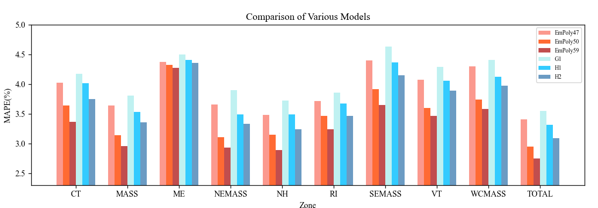
Figure 4: The performance comparision of $G_{1}$, $H_{1}$, $H_{2}$, HOPS47, HOPS50 and HOPS59. $G_{1}$ and HOPS47, $H_{1}$ and HOPS50, $H_{2}$ and HOPS59 essentially share the same information, respectively. The forecasting accuracy of these models generally improves as the number of variables increases. However, when the input information keeps the same, our model consistently outperforms the existing models $G_{1}$, $H_{1}$ and $H_{2}$, respectively.

IV-F Extension Experiments Compared with the Recency Model

Our polynomial model operates independently of variable selection, which implies that it can be integrated with other existing variable selection based models to further enhance forecasting accuracy. We take the Recency model as an example for further discussion.

As an enhanced variable selection based model for load forecasting, the Recency model [20] demonstrates greater effectiveness compared to the vanilla model $G_{1}$ and many other load forecasting models. It mainly selects appropriate lagged hourly temperatures and/or moving average temperatures in order to capture the recency effect fully. The daily moving average temperature of the $d$-th day can be written as:

$$\widetilde{T}_{t,d}=\frac{1}{24}\sum^{24d}_{h=24d-23}T_{t-h},d=1,2,3\cdots,$$

and the Recency model can be expressed as:

$$y_{t}= r_{0}+r_{1}Trend_{t}+r_{2}H_{t}+r_{3}W_{t}+r_{4}M_{t}$$

$$+r_{5}H_{t}W_{t}+\sum_{h}f(T_{t-h})+\sum_{d}f(\widetilde{T}_{t,d}),$$

where $h$ and $d$ can be selected by the validation set. Similar to the Recency model, we also incorporate the recency effect variables $T_{t-i},T_{t-i}^{2},T_{t-i}^{3},(0\leq i\leq h)$ and $\widetilde{T}_{t,j},\widetilde{T}_{t,j}^{2},\widetilde{T}_{t,j}^{3},(1\leq j\leq d)$ in our HOPS model, and we choose the following grid search range:$\{0,1,2,3,\cdots,24\}$ for $h$ and $\{1,2,3,\cdots,7\}$ for $d$. The difference is that we do not include interaction terms as variables so that we take use less and simpler variables. We denote it as ReHOPS (the Recency HOPS Model). For practicality and reducing training time, we fix $k_{2}=60$ and $k_{3}=9$. This may not be the optimal choice for $k_{2}$ and $k_{3}$, but generally, the forecasting performance is not highly sensitive to the embedding dimension.

We first train the model on the data of 2012 and 2013. Then, we select the optimal h-d pair using the data of 2014. Finally, we retrain the model on the data of 2013 and 2014, then forecast on 2015. We use two years of data for retraining instead of, as before, three years, in order to maintain consistency with [20]. Both Recency and ReHOPS use the above process to select variables. The experimental results are presented in Table III. It can be observed that our model demonstrates a significant improvement over the Recency model.

Finally, to demonstrate the practicality of the proposed method, we list the total training and forecasting time of 10 datasets for each model as Table IV.

TABLE III: Comparisons Between the Recency model and the HOPS model. ReEm represents ReHOPS and Rece represents Recency.

					Daily Peak
	MAPE(%)		MSE (×103)		MAPE(%)
Zone	ReHOPS	Recency	ReHOPS	Recemcy	ReHOPS	Recency
CT	3.01	3.31	20.65	25.80	2.75	3.33
MASS	2.84	3.39	66.00	102.16	2.56	3.19
ME	4.50	4.84	5.00	6.15	3.81	3.73
NEMASS	3.20	3.60	17.96	24.61	3.06	3.70
NH	2.66	2.92	2.46	3.10	2.63	2.89
RI	2.89	3.28	1.48	2.17	2.72	3.17
SEMASS	3.50	3.89	6.39	8.96	2.82	3.50
VT	4.11	4.06	1.09	1.03	3.13	3.29
WCMASS	3.41	3.68	8.34	10.36	3.08	3.51
AVERAGE	3.35	3.66	14.37	20.48	2.95	3.37
TOTAL	2.42	2.74	220.55	313.32	2.30	2.66

TABLE IV: The total time taken by proposed models.

Model	HOPS289	HOPS47	HOPS50	HOPS59	ReHOPS
Time	1h6m9s	19m24s	20m53s	26m26s	2h28m42s

V Conclusion

In this paper, we propose a high-order polynomial forecasting model with self-supervised dimension reduction (HOPS), which results in stable improvements in load forecasting accuracy. Additionally, we introduce a fast algorithm based on FR-CG, significantly enhancing the efficiency of solving the numerical optimization problem. The results of our numerical experiments also demonstrate that our method can achieve higher forecast accuracy with fewer parameters and less complex variable combinations than its counterparts.

More importantly, our approach can be integrated with many existing load forecasting methods. While numerous existing schemes rely on the selection and inclusion of additional influential variables, our method does not depend on variable selection. If additional variables are identified as driving factors of the load, they can be incorporated into our proposed framework to further improve forecast accuracy.

References

- [1] R. Weron, Modeling and forecasting electricity loads and prices: A statistical approach. John Wiley & Sons, 2006, vol. 396.
- [2] T. Hong and S. Fan, “Probabilistic electric load forecasting: A tutorial review,” International Journal of Forecasting, vol. 32, no. 3, pp. 914–938, 2016.
- [3] H. S. Hippert, C. E. Pedreira, and R. C. Souza, “Neural networks for short-term load forecasting: A review and evaluation,” IEEE Transactions on power systems, vol. 16, no. 1, pp. 44–55, 2001.
- [4] Y. Wang, Q. Chen, T. Hong, and C. Kang, “Review of smart meter data analytics: Applications, methodologies, and challenges,” IEEE Transactions on Smart Grid, vol. 10, no. 3, pp. 3125–3148, 2018.
- [5] N. Charlton and C. Singleton, “A refined parametric model for short term load forecasting,” International Journal of Forecasting, vol. 30, no. 2, pp. 364–368, 2014.
- [6] T. Hong, J. Wilson, and J. Xie, “Long term probabilistic load forecasting and normalization with hourly information,” IEEE Transactions on Smart Grid, vol. 5, no. 1, pp. 456–462, 2013.
- [7] I. Dimoulkas, P. Mazidi, and L. Herre, “Neural networks for gefcom2017 probabilistic load forecasting,” International Journal of Forecasting, vol. 35, no. 4, pp. 1409–1423, 2019.
- [8] J. Xie, Y. Chen, T. Hong, and T. D. Laing, “Relative humidity for load forecasting models,” IEEE Transactions on Smart Grid, vol. 9, no. 1, pp. 191–198, 2016.
- [9] B.-J. Chen, M.-W. Chang et al., “Load forecasting using support vector machines: A study on eunite competition 2001,” IEEE transactions on power systems, vol. 19, no. 4, pp. 1821–1830, 2004.
- [10] J. Luo, T. Hong, Z. Gao, and S.-C. Fang, “A robust support vector regression model for electric load forecasting,” International Journal of Forecasting, vol. 39, no. 2, pp. 1005–1020, 2023.
- [11] T. Hong, P. Pinson, and S. Fan, “Global energy forecasting competition 2012,” pp. 357–363, 2014.
- [12] J. Xie and T. Hong, “Gefcom2014 probabilistic electric load forecasting: An integrated solution with forecast combination and residual simulation,” International Journal of Forecasting, vol. 32, no. 3, pp. 1012–1016, 2016.
- [13] T. Hong, J. Xie, and J. Black, “Global energy forecasting competition 2017: Hierarchical probabilistic load forecasting,” International Journal of Forecasting, vol. 35, no. 4, pp. 1389–1399, 2019.
- [14] F. Ziel and B. Liu, “Lasso estimation for gefcom2014 probabilistic electric load forecasting,” International Journal of Forecasting, vol. 32, no. 3, pp. 1029–1037, 2016.
- [15] J. Xie and T. Hong, “Gefcom2014 probabilistic electric load forecasting: An integrated solution with forecast combination and residual simulation,” International Journal of Forecasting, vol. 32, no. 3, pp. 1012–1016, 2016.
- [16] S. Haben and G. Giasemidis, “A hybrid model of kernel density estimation and quantile regression for gefcom2014 probabilistic load forecasting,” International Journal of Forecasting, vol. 32, no. 3, pp. 1017–1022, 2016.
- [17] J. Nowotarski, B. Liu, R. Weron, and T. Hong, “Improving short term load forecast accuracy via combining sister forecasts,” Energy, vol. 98, pp. 40–49, 2016.
- [18] J. R. Lloyd, “Gefcom2012 hierarchical load forecasting: Gradient boosting machines and gaussian processes,” International Journal of Forecasting, vol. 30, no. 2, pp. 369–374, 2014.
- [19] S. B. Taieb and R. J. Hyndman, “A gradient boosting approach to the kaggle load forecasting competition,” International journal of forecasting, vol. 30, no. 2, pp. 382–394, 2014.
- [20] P. Wang, B. Liu, and T. Hong, “Electric load forecasting with recency effect: A big data approach,” International Journal of Forecasting, vol. 32, no. 3, pp. 585–597, 2016.
- [21] H. Hahn, S. Meyer-Nieberg, and S. Pickl, “Electric load forecasting methods: Tools for decision making,” European journal of operational research, vol. 199, no. 3, pp. 902–907, 2009.
- [22] J. Xie and T. Hong, “Variable selection methods for probabilistic load forecasting: Empirical evidence from seven states of the united states,” IEEE Transactions on Smart Grid, vol. 9, no. 6, pp. 6039–6046, 2017.
- [23] T. Hong, Short term electric load forecasting. North Carolina State University, 2010.
- [24] Y. Saad, Iterative methods for sparse linear systems. SIAM, 2003.
- [25] G. H. Golub and C. F. Van Loan, Matrix computations. JHU press, 2013.
- [26] R. Fletcher and C. M. Reeves, “Function minimization by conjugate gradients,” The computer journal, vol. 7, no. 2, pp. 149–154, 1964.