Evidence for Jet/Outflow Shocks Heating the Environment Around the Class I Protostellar Source Elias 29: FAUST XXI

Abstract

We have observed the late Class I protostellar source Elias 29 at a spatial-resolution of 70 au with the Atacama Large Millimeter/submillimeter Array (ALMA) as part of the FAUST Large Program. We focus on the line emission of SO, while that of ³⁴SO, C¹⁸O, CS, SiO, H¹³CO⁺, and DCO⁺ are used supplementally. The spatial distribution of the SO rotational temperature ($T_{\rm rot}$(SO)) is evaluated by using the intensity ratio of its two rotational excitation lines. Besides in the vicinity of the protostar, two hot spots are found at a distance of 500 au from the protostar; $T_{\rm rot}$(SO) locally rises to 53${}^{+25}_{-15}$ K at the interaction point of the outflow and the southern ridge, and 72${}^{+66}_{-29}$ K within the southeastern outflow probably due to a jet-driven bow shock. However, the SiO emission is not detected at these hot spots. It is likely that active gas accretion through the disk-like structure and onto the protostar still continues even at this evolved protostellar stage, at least sporadically, considering the outflow/jet activities and the possible infall motion previously reported. Interestingly, $T_{\rm rot}$(SO) is as high as 20$-$30 K even within the quiescent part of the southern ridge apart from the protostar by 500$-$1000 au without clear kinematic indication of current outflow/jet interactions. Such a warm condition is also supported by the low deuterium fractionation ratio of HCO⁺ estimated by using the H¹³CO⁺ and DCO⁺ lines. The B-type star HD147889 $\sim$0.5 pc away from Elias 29, previously suggested as a heating source for this region, is likely responsible for the warm condition of Elias 29.

1 Introduction

1.1 Background

A wide variety of planetary systems have been discovered in recent decades (e.g. Andrews et al., 2018; Öberg et al., 2021). The origin of their diversity, both in the physics and chemistry, probably resides in the earliest history of the planetary system formation; namely, what happened during the protostellar phases. Thus, it is important to investigate this phase for thorough understanding of star and planet formation and its diversity. In this phase, gas accretion to the protostar and dissipation of surrounding gas are simultaneously ongoing, so that a parent core generally reveals a very complex structure. Recent ALMA observations have indeed delineated a detailed view of the complex physical and chemical nature of protostellar sources at a high angular resolution (e.g. Tokuda et al., 2014; van der Wiel et al., 2019; Okoda et al., 2021; Ohashi et al., 2022; Codella et al., 2024). In both gas accretion and dissipation, the outflow/jet plays a central role (e.g. Bachiller, 1996; Bally, 2016).

First, outflows are known to be important mechanisms for removing angular momentum from the gas accreting onto the protostar, and therefore closely connected to the formation of the disk/envelope system and the growth of protostars (e.g. Blandford & Payne, 1982; Tomisaka, 2000; Machida et al., 2008; Hirota et al., 2017; Machida & Basu, 2019). Second, the outflow plays a crucial role in the dissipation of the parent core, the details of which are still an open issue of theoretical study (e.g. Offner & Chaban, 2017; Nakamura & Li, 2014). The outflow evolution is thus important for both regulation and feedback processes in the formation of a star and the circumstellar environment. Hence, outflows have extensively been studied by radio observations, particularly for early-stage protostars (e.g. Lee et al., 2000; Arce & Sargent, 2006; Hatchell et al., 2007; Curtis et al., 2010; Matsushita et al., 2019; Nakamura et al., 2011a; Oya et al., 2014, 2015, 2018a, 2018b, 2021; Omura et al., 2024). Furthermore, it is known that the chemical composition of a parent core is greatly affected by the outflow activity (e.g. Mikami et al., 1992; Bachiller & Pérez Gutiérrez, 1997; Bachiller et al., 2001; Arce et al., 2008; Codella et al., 2010; Ceccarelli et al., 2010, 2017; Sugimura et al., 2011; Podio et al., 2017). Hence, the outflow stands for a key phenomenon to disentangle complex physical and chemical structure of protostellar cores.

On the other hand, observational studies of outflows and their feedback on the chemical evolution of evolved protostars at the late Class I stage are relatively sparse, especially at high angular resolution (e.g. Le Gal et al., 2020; Bianchi et al., 2022; Tanious et al., 2024). This is in part due to the lower mass accretion rates associated with evolved protostars, which generally drive less powerful and fainter outflows (e.g. Machida & Hosokawa, 2013). Therefore, it is important to investigate additional sources at the late evolutionary stage, to attain a more thorough understanding of both the outflow evolution and its feedback to the parent core. Even if the outflow feature is faint, temperature structure as well as chemical structure around the protostar would tell us important information on the outflow activity. Moreover, accreted material at the late evolutionary stage remains in the disk and could have an outsize contribution to planets and comets. Thus, the nature of the late-accreting material would affect the chemical composition of comets; for instance, a supply of warm material could result in lower deuterium fractionation in comets than in the dense interstellar medium. Given these needs, we included the relatively evolved protostellar source Elias 29 in our ALMA large program FAUST (Fifty AU Study of the chemistry in the disk/envelope system of solar-like protostars; 2018.1.01205.L; P.I.: S. Yamamoto). FAUST aims to delineate physical and chemical structures of 13 protostellar sources at a spatial resolution of $\sim$50 au (Codella et al., 2021b; Oya et al., in prep.).

1.2 Target Source: Elias 29

Elias 29, also known as WL 15 (Wilking & Lada, 1983), is a Class I protostar in the L1688 dark cloud within the Ophiuchus star-forming region ($d=137$ pc; Ortiz-León et al., 2017). Lommen et al. (2008) reported a bolometric temperature and bolometric luminosity of 391 K and 13.6 $L_{\odot}$, respectively. The systemic velocity of the protostellar system is about 4 km s^-1 (Oya et al., 2019). Elias 29 is surrounded by many YSOs, making the environment of this source very complex (Rocha & Pilling, 2018).

Previous observational studies of Elias 29 at $>$$10^{4}$ au scale have focused on its outflow structure (Sekimoto et al., 1997; Ceccarelli et al., 2002; Ybarra et al., 2006; Bussmann et al., 2007; Nakamura et al., 2011b; van der Marel et al., 2013). According to CO ($J=3-2$) observations with Heinrich Hertz Telescope by Bussmann et al. (2007), the outflow has an inverse S-like shape at a 4000 au scale. The S-like structure is presumably due to a temporal change in the outflow direction. On a smaller scale around the protostar, Ceccarelli et al. (2002) detected the outflow in CO ($J=6-5$) emission with the James Clerk Maxwell Telescope, noting that the blue-shifted and red-shifted lobes are on the west and east sides of the protostar, respectively. In addition, the protostellar jet was observed in the near-infrared by Ybarra et al. (2006), revealing H₂ knots produced by the precessing east-west jet, consistent with the outflow morphology found by Ceccarelli et al. (2002) and Bussmann et al. (2007).

The gas structures observed in Elias 29 at $<$$10^{3}$ au scale consist of two main components, according to the observations of various molecular lines by Lommen et al. (2008) and Oya et al. (2019). These are a compact central component associated to the protostar and an off-center dense gas clump (called the “southern ridge” hereafter). The southern ridge is $\sim$500 au ($\sim$4″) south of the protostar and extends along the northeast-southwest direction, and its origin is unclear at the moment (Lommen et al., 2008; Oya et al., 2019). Oya et al. (2019) observed Elias 29 in SO and SO₂ emission with ALMA, reporting rotational motion for the compact component associated to the protostar. The authors estimated the protostellar mass to be from 0.8 to 1.0 $M_{\odot}$, assuming Keplerian motion, and a disk inclination angle from 65° to 90° (0° for face-on).

The molecular gas within Elias 29 is reported to show peculiar chemical characteristics (Oya et al., 2019). According to their results, the SO and SO₂ emission is very bright in the compact component around the protostar. The compact distribution of SO₂ in this source has also been reported by Artur de la Villarmois et al. (2019). Such compact distributions of SO and SO₂ have been reported for a few other sources (e.g. SVS 13 by Codella et al. 2021a and Bianchi et al. 2023; Oph IRS 44 by Artur de la Villarmois et al. 2022). On the other hand, CS emission, which for systems with typical chemical characteristics is usually bright within the disk/envelope system (e.g. Oya et al., 2015, 2017; Imai et al., 2016), is faint toward the continuum peak and is preferentially seen within the southern ridge. Both of the components are deficient in interstellar complex organic molecules (iCOMs), such as HCOOCH₃ and (CH₃)₂O, and unsaturated hydrocarbon molecules, such as CCH and c-C₃H₂. As a possible explanation for these chemical characteristics, Oya et al. (2019) proposed a relatively high dust temperature ($\geq$20 K) in the parent cloud; dust surface reactions to form the above molecular species would be insufficient because such a high dust temperature prevents their mother species (e.g., C and CO) from depletion onto dust grains (see Section 5.2; Oya, 2022). Indeed, Rocha & Pilling (2018) reported that the parent cloud of Elias 29 is irradiated by two bright BV stars, S1 and HD 147889; their model calculation suggested that the gas temperature of the cloud should not have been below 20 K. The actual temperature in the environment around the protostar, however, has not been delineated observationally so far; therefore, we firstly delineate the temperature distribution in Elias 29 at a $10^{2-3}$ au scale in this project.

In this paper, we focus on the distribution of the rotational temperature of SO by using two SO lines in ALMA Band 6. The details of the observations are given in Section 2. Section 3 describes the overall view of the observational results, including the findings of hot regions. The hot regions are also found to be characteristic in gas dynamics (Section 4); we discuss the feedback induced by the outflow (Section 4.1) and jet (Section 4.2) activities in this source as the candidate cause for the local heating of the gas apart from the protostar. The mass accretion is discussed in Section 4.3. The chemical composition of this source is explored in Section 5. The SO column density is evaluated in Section 5.1 and found not to be significantly enhanced by the shock chemistry. As a support for the warm environment of this source, the deuterium fractionation ratio of HCO⁺ is discussed by using the H¹³CO⁺ and DCO⁺ emissions in Section 5.2. Section 6 gives the summary of this paper.

2 Observation

With ALMA, we observed the field around Elias 29 between 2018 October and 2020 March during Cycle 6 operation, as part of the ALMA large program FAUST (2018.1.01205.L). Spectral lines listed in Table Evidence for Jet/Outflow Shocks Heating the Environment Around the Class I Protostellar Source Elias 29: FAUST XXI were observed in Band 6 using two frequency ranges, Setup 1 (214.0$-$219.0 GHz, 229.0$-$234.05 GHz) and Setup 2 (242.5$-$247.5 GHz, 257.5$-$262.5 GHz). In each spectral setup, we used the 12-m array data with two different antenna configurations, C43-4 and C43-1, as well as the 7-m array data of the Atacama Compact Array (ACA/Morita Array). Both Setups 1 and 2 were observed by 12 spectral windows with the bandwidth and the frequency resolution of 59 MHz and 122 kHz (0.15 km s^-1 at 250 GHz), respectively, and one with the bandwidth and the frequency resolution of 1875 MHz and 1.129 MHz (1.4 km s^-1 at 250 GHz), respectively. The basic parameters of the observations including calibrator sources are summarized in Table Evidence for Jet/Outflow Shocks Heating the Environment Around the Class I Protostellar Source Elias 29: FAUST XXI. The field center of the observations was ($\alpha_{\rm ICRS}$, $\delta_{\rm ICRS}$) $=$ ($16^{\rm h}27^{\rm m}09.\!\!^{\rm s}437$, $-24\arcdeg 37\arcmin 19\farcs 304$). The system temperature ($T_{\rm sys}$) was typically 70$-$130 K during the observations. The data were reduced using the Common Astronomy Software Applications (CASA) package (CASA Team et al., 2022) utilizing a modified version of the ALMA calibration pipeline based on v.5.6.1-8.el7 and an additional in-house calibration routine to correct for the $T_{\rm sys}$ and spectral line data normalization. Self-calibration was carried out using line-free continuum emission for each configuration. Details of the self-calibration process are described by Imai et al. (2022). The visibility data with the three different configurations were combined in the UV plane after the self-calibration. The absolute accuracy of the flux calibration was 10% (Warmels et al., 2018). Images of C¹⁸O ($J=2-1$), SO ($J_{N}=6_{5}-5_{4}$), SO ($J_{N}=6_{6}-5_{5}$), ³⁴SO ($J_{N}=5_{6}-4_{5}$), CS ($J=5-4$), SiO ($J=5-4$), H¹³CO⁺ ($J=3-2$), and DCO⁺ ($J=3-2$) were obtained with the CLEAN algorithm of CASA (v.5.7.2-4) by employing Briggs weighting with a robustness parameter of 0.5. The beam size of the line emission is about $0\farcs 5\times 0\farcs 4$ by combining the data with all the antenna configurations (C43-4, C43-1, and ACA) as summarized in Table Evidence for Jet/Outflow Shocks Heating the Environment Around the Class I Protostellar Source Elias 29: FAUST XXI. The maximum recoverable scale of the observation with the ACA is 30$\farcs$3 according to the QA2 report. The images are corrected for the primary beam attenuation.

3 Results

3.1 Overall Morphology

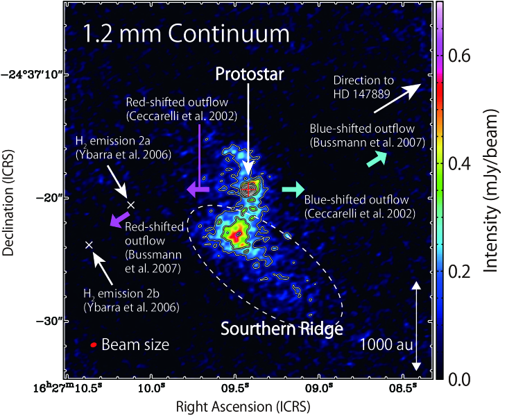
Figure 1: 1.2 mm continuum map. The red cross represents the continuum peak position at the location of the Elias 29 protostar, where the peak intensity is 15 mJy beam^-1. The southern ridge component is indicated by the white dashed ellipse. Contour levels are every two times starting from 5$\sigma$ (i.e. 5$\sigma$, 10$\sigma$, 20$\sigma$, …), where $\sigma$ of 30 $\mu$Jy beam^-1 is the rms noise level. The beam size is shown in the red ellipse at the bottom left corner of the map. Magenta and cyan arrows represent the directions of the red-shifted and blue-shifted outflow lobes, respectively, previously reported by Ceccarelli et al. (2002) and Bussmann et al. (2007). White crosses represent the positions where the H₂ emission was reported by Ybarra et al. (2006). White arrow on the northwestern side of the panel represents the direction to the B-type star HD 147889 taken from Rocha & Pilling (2018).

Figure 1 shows the 1.2 mm continuum map of Elias 29. The continuum emission has its brightest peak at the protostar position. The continuum peak position is derived to be ($\alpha_{\rm ICRS}$, $\delta_{\rm ICRS}$) $=$ ($16^{\rm h}27^{\rm m}09.\!\!^{\rm s}41737\pm 0.\!\!^{\rm s}00007$, $-24\arcdeg 37\arcmin 19\farcs 3104\pm 0\farcs 0007$) with a peak flux density of $14.62\pm 0.06$ mJy beam^-1 based on 2-dimensional Gaussian fitting task imfit with CASA for the continuum image. The convolved and deconvolved sizes of the continuum emission are $(0\farcs 550\pm 0\farcs 003)\times(0\farcs 404\pm 0\farcs 001)$ and $(0\farcs 165\pm 0\farcs 009)\times(0\farcs 152\pm 0\farcs 005)$, respectively, where the synthesized beam size is $0\farcs 52\times 0\farcs 37$ (PA $=$ $-70.\!\!\arcdeg 0$). Besides this intensity peak, we found a weak north-south extension with a moderate emission peak of 0.63 mJy beam^-1 at 600 au southeast of the protostar, which belongs to the southern ridge component. Although this weak emission was not detected in Oya et al. (2019), it was detected in this project likely thanks to both the higher sensitivity and the wider UV coverage from the inclusion of an ACA configuration. Scientific examination based on the continuum emission, including the 3 mm data taken as part of the FAUST program as well as the 1.2 mm data used here, will be reported separately.

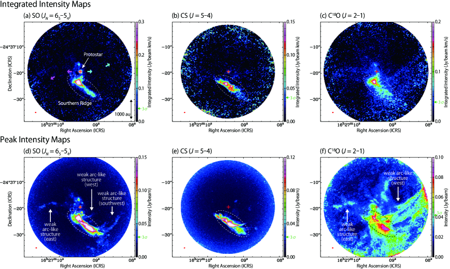
Figure 2: (a,b,c) Integrated intensity (moment 0) maps of SO ($J_{N}=6_{5}-5_{4}$), CS ($J=5-4$), and C¹⁸O ($J=2-1$), respectively. The velocity range for the integration is from $-20$ to 30 km s^-1. (d, e, f) Peak intensity (moment 8) maps of the three molecular lines. The velocity range taken into account is from $-20$ to 30 km s^-1. The red cross in each panel represents the continuum peak position: ($\alpha_{\rm ICRS}$, $\delta_{\rm ICRS}$) $=$ ($16^{\rm h}27^{\rm m}09.\!\!^{\rm s}41737\pm 0.\!\!^{\rm s}00007$, $-24\arcdeg 37\arcmin 19\farcs 3104\pm 0\farcs 0007$). The red ellipse at the bottom left corner in each panel represents the beam size for each molecular line. The magenta and cyan arrows in the top left panel are the same as those in Figure 1. White and black dotted ellipses indicate the southern ridge component. Green arrow indicates the 3$\sigma$ noise level in the color bar.

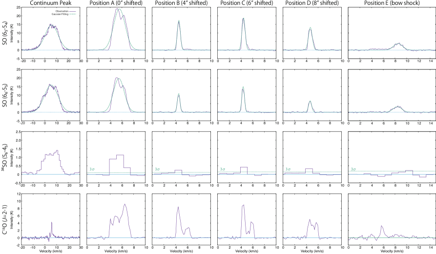
Figure 3: Spectra of the SO ($J_{N}=6_{5}-5_{4}$, $J_{N}=6_{6}-5_{5}$) and ³⁴SO ($J_{N}=5_{6}-4_{5}$) lines at Positions A$-$E (Figure 4). Coordinates of the Positions A$-$E are summarized in Table Evidence for Jet/Outflow Shocks Heating the Environment Around the Class I Protostellar Source Elias 29: FAUST XXI. Each spectrum is obtained as the average over the circular region with a diameter of 1″ centered at each of Positions A$-$D, while the spectrum at one pixel is employed for Position E. A frequency resolution of ³⁴SO ($J_{N}=5_{6}-4_{5}$) data is 1.129 MHz, while that of the other molecular line data is 141 kHz.

Figure 2 shows the integrated and peak intensity maps of the SO ($J_{N}=6_{5}-5_{4}$), CS ($J=5-4$), and C¹⁸O ($J=2-1$) lines. The southern ridge component is bright in all the three species, while the continuum peak position is bright only in the SO emission. The distribution of SO and CS are confirmed to be consistent with that previously reported by Oya et al. (2019) with a higher spatial resolution and sensitivity of our data. The distribution of C¹⁸O is found to be extended over the field of view and relatively weak at the continuum peak. The C¹⁸O emission is generally more extended than the SO emission. Hence, the former can be more filtered out by the interferometer, although the maximum recoverable scale of 30$\farcs$3 will contribute to recover the extended emission. Even if the C¹⁸O emission were resolved out for the systemic velocity component due to contamination of the extended ambient component, the high velocity-shift components originating from the spin-up velocity structure near the protostar (Hartmann, 2008; Ohashi et al., 2014; Oya et al., 2022) should be detected as seen for the SO lines (Figure 3; see Section 3.2). In addition, a compact distribution should also be seen toward the protostar in the peak intensity map. A lack of these features (Figures 2f, 3) indicates that the C¹⁸O emission is not resolved out significantly but is really weak around the protostar. The peak intensity map of the C¹⁸O emission seems to have voids towards the northwest and southeast of the continuum peak position. This observed structure is likely related to the cavity produced by the outflow extending along the northwest-southeast direction (Ceccarelli et al., 2002; Ybarra et al., 2006; Bussmann et al., 2007), as discussed further in Section 4.1. We also note weak arc-like structures in the peak intensity map of the SO emission (Figure 2d) with the intensity up to 51 mJy beam^-1 detected by $\sim$5$\sigma$, where $\sigma$ of 10 mJy beam^-1 is the rms noise level; the features on the eastern and western sides may trace the southeast and northwest outflow cavity walls, respectively (See also Section 4.1). Meanwhile, that on the southwestern side morphologically seems to be related to the southern ridge component.

3.2 Temperature Distribution

In this section we investigate the distribution of the rotational temperature of SO by using its two observed transitions ($J_{N}=6_{5}-5_{4}$, $E_{\rm u1}=35$ K; $J_{N}=6_{6}-5_{5}$, $E_{\rm u2}=57$ K). Assuming the LTE (local thermodynamic equilibrium) and optically thin conditions, the rotational temperature ($T_{\rm rot}$) of SO is derived from the ratio of the integrated intensities of its two lines according to the following equation:

$$\frac{W_{2}}{W_{1}}=\frac{\nu_{1}(S\mu^{2})_{2}}{\nu_{2}(S\mu^{2})_{1}}\exp\left(-\frac{E_{\rm u2}-E_{\rm u1}}{k_{\rm B}T_{\rm rot}}\right),$$ (1)

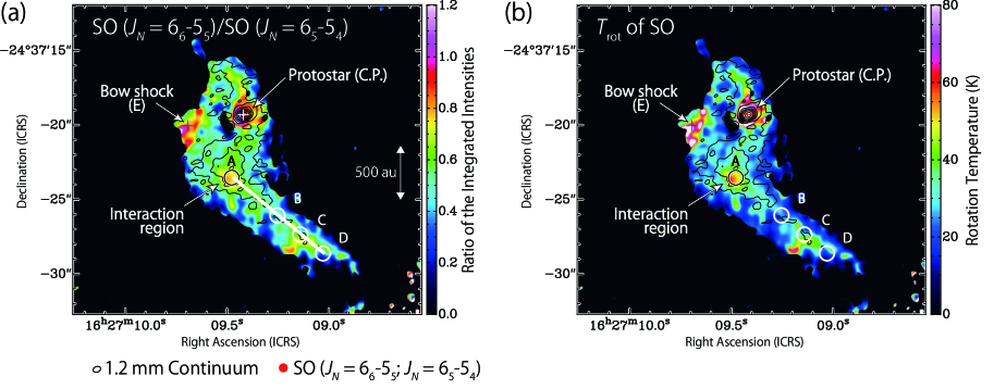
Figure 4: Maps of (a) the ratio of the integrated intensities of the two SO lines (b) and the rotational temperature of SO derived from the intensity ratio. The images of the two SO lines are smoothed so that their beam sizes are to be $0\farcs 6\times 0\farcs 6$, as shown by the red circle outside the panels. The velocity range for the integration is from $-15$ to $+23$ km s^-1. Black contours in each panel represent the 1.2 mm continuum emission, where the contour levels are the same as those in Figure 1. The beam size of the continuum image is shown by a black ellipse outside the panels. (a) Ratio of the integrated intensity of the SO ($J_{N}=6_{6}-5_{5}$) line to the SO ($J_{N}=6_{5}-5_{4}$) line, which corresponds to $W_{2}/W_{1}$ in Equation (1). The pixels where the integrated intensity of the SO ($J_{N}=6_{5}-5_{4}$) line is less than 2$\sigma$ are shown in black, where $\sigma$ of 18 mJy beam^-1 is the rms noise level. (b) Rotational temperature of SO derived from the ratio of the integrated intensity of the two line emissions in the panel (a). The pixels with negative values are shown in black, where the ratio of the integrated intensity is less than 0 or higher than the high temperature limit ($1.15$ for $T_{\rm rot}=\infty$). See the footnotes for Table Evidence for Jet/Outflow Shocks Heating the Environment Around the Class I Protostellar Source Elias 29: FAUST XXI for the explanation about Positions A-E.

where $W$ is the observed integrated intensity, $\nu$ the frequency of the transition, $S$ the line strength, $\mu$ the dipole moment responsible for the transition, and $E_{\rm u}$ the upper-state energy. The $\nu$, $S\mu^{2}$, and $E_{\rm u}$ values for each line are listed in Table Evidence for Jet/Outflow Shocks Heating the Environment Around the Class I Protostellar Source Elias 29: FAUST XXI, which are taken from CDMS (The Cologne Database for Molecular Spectroscopy; Müller et al., 2005; Endres et al., 2016). Suffixes, 1 and 2, represent the $J_{N}=6_{5}-5_{4}$ and $J_{N}=6_{6}-5_{5}$ transitions, respectively. Figure 4(a) shows the map of the ratio of the integrated intensities of the two SO lines, and Figure 4(b) shows the map of the evaluated $T_{\rm rot}$ of SO.

The $T_{\rm rot}$ is mostly 20$-$30 K in the southern ridge component, except for a few small localized spots. We found three regions with a high rotational temperature in Figure 4(b); the component around the continuum peak position labeled as ‘C.P.’, the position at 500 au south of the protostar labeled as ‘Position A’ in the southern ridge component, and that at 500 au east of the protostar labeled as ‘Position E’. Here, we specifically investigate the rotational temperature for these three positions and additional three positions in the southern ridge (Positions B, C, and D). The coordinates of these positions are summarized in Table Evidence for Jet/Outflow Shocks Heating the Environment Around the Class I Protostellar Source Elias 29: FAUST XXI. These positions are indicated on the maps in Figure 4. Positions A$-$D are taken to be aligned on the white line along the extension of the southern ridge component in Figure 4(a). Their central positions are separated by 2″ from each other with an exception, the position between Position A and Position B, due to a complex velocity structure. Figure 3 shows the spectra of the SO lines observed at Positions A$-$E and C.P..

The observed line parameters of SO for these positions are summarized in Table Evidence for Jet/Outflow Shocks Heating the Environment Around the Class I Protostellar Source Elias 29: FAUST XXI. Here, the spectra at Positions A$-$D are averaged over a circular region with a diameter of 1″ to increase the S/N ratio, while those at Position E are taken at just 1 pixel to trace the compact structure of the bow-shocked region. The line profiles are generally asymmetric and deviate from the Gaussian shape (Figure 3). Thus, we do not employ the Gaussian fitting to derive the line parameters except for Position E. For instance, the peak intensity of each line is evaluated from the peak value of the line profile (see the footnote of Table Evidence for Jet/Outflow Shocks Heating the Environment Around the Class I Protostellar Source Elias 29: FAUST XXI for details).

From the integrated intensities of the two SO lines, the rotational temperature of SO at Positions A$-$E and the continuum peak are derived by using Equation (1), as listed in Table Evidence for Jet/Outflow Shocks Heating the Environment Around the Class I Protostellar Source Elias 29: FAUST XXI. Since we use the integrated intensities in this analysis, the results do not suffer from the asymmetry of the line profile. We discuss a possible cause for the high temperature at Positions A (53${}^{+25}_{-15}$ K) and E (72${}^{+66}_{-29}$ K) in Sections 4.1 and 4.2, respectively. Although there is also another candidate spot with a high rotational temperature ($>60$ K) on the southern side of ‘Position C’, this result severely suffers from the error for the weak SO intensities; for instance, the rotational temperature is reduced to be 28 K by accounting for the 3$\sigma$ error (45 mJy beam^-1 km s^-1) of the SO ($J_{N}=6_{6}-5_{5}$) line integrated intensity.

Since the evaluation of $T_{\rm rot}$ may suffer from the simple assumptions of the LTE and optically thin conditions, we confirmed its validity using a non-LTE analysis for Positions A$-$E. We used the two SO lines data and one ³⁴SO line data to constrain the three free parameters (the gas kinetic temperature, the SO column density, and the H₂ number density) by the $\chi^{2}$ method. We employed the photon-escaping probability for a static, spherically symmetric, and homogeneous medium (Osterbrock & Ferland, 2006; van der Tak et al., 2007). The spectra of the SO and ³⁴SO lines used for the non-LTE analysis are shown in Figure 3 for Positions A$-$E, whose parameters are summarized in Table Evidence for Jet/Outflow Shocks Heating the Environment Around the Class I Protostellar Source Elias 29: FAUST XXI. Further details for the non-LTE analysis are described in Appendix A.

4 Outflow/Jet Feedback as Candidate Causes for the Local Heating

4.1 Temperature Enhancement due to Outflow Interactions

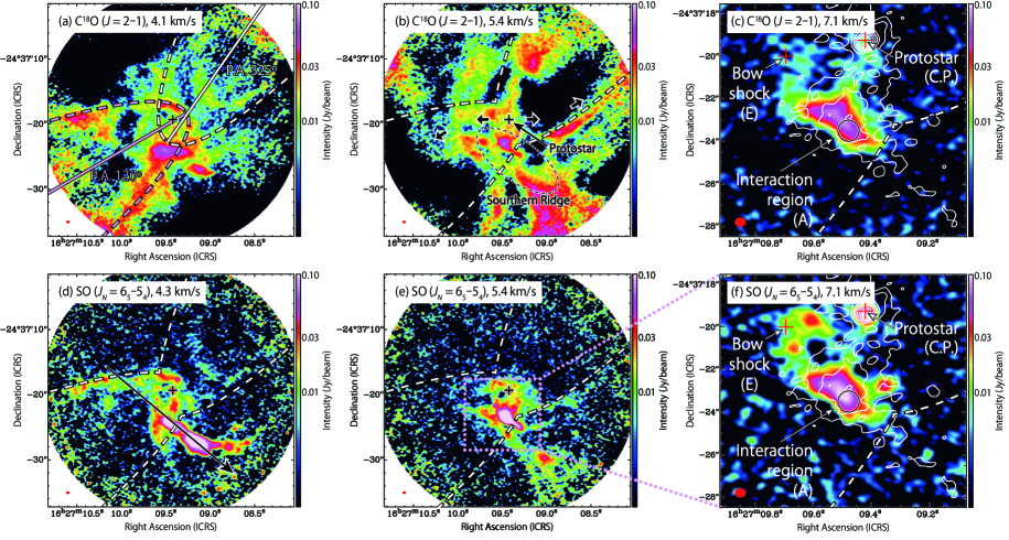
Figure 5: The velocity channel maps of the C¹⁸O ($J=2-1$; a$-$c) and SO ($J_{N}=6_{5}-5_{4}$; d$-$f) lines. Panels (a, d) show the velocity channel maps of the two molecular lines near the systemic velocity of the protostar ($\sim$$+4$ km s^-1). Panels (b, e) show their velocity channel maps with the red-shifted velocity (5.4 km s^-1). Panels (c, f) show the maps with a more red-shifted velocity (7.1 km s^-1), focusing on the region around Position A. The pink dotted rectangle in panel (e) indicates the region shown in panels (c, f). White contours in panels (c, f) represent the continuum emission, where the contour levels are the same as those in Figure 1. The beam size is depicted by a red ellipse at the bottom left corner in each panel. Black or red cross in each panel represents the protostellar position (C.P.). White and pink dashed lines indicate the outflow morphology obtained based on these panels. The central axes of the parabolic shapes are represented by white and pink solid lines in panel (a), which have the position angles of 120° and 325°, respectively. The directions of the outflow lobes previously reported are indicated by the black arrows in panel (c), which are the same as the magenta and cyan arrows in Figure 1. Black arrow in panel (d) indicates the position axis along which Figure 6 is obtained.

In this section, we discuss the region’s interaction with the outflow as the potential cause for the high temperature at Position A. Figure 5 shows the velocity channel maps of the C¹⁸O and SO emissions. Although the overall structure is complex, we find a part of a parabolic feature extending over 20″ ($\sim$2700 au) oriented toward southeast from the protostar in Figures 5(a, b, d). We see a void of the C¹⁸O emission in its velocity channel map of $+5.4$ km s^-1 (Figure 5b) inside the parabolic shape on the northwestern side of the protostar, while such a feature is not evident in the SO emission (Figure 5e). This feature is seen probably because the C¹⁸O emission traces the cavity wall of the northwestern outflow lobe.

The outflow of this source was previously reported based on the single-dish CO ($J=6-5$) observation by Ceccarelli et al. (2002), where the outflow axis is extending along the east-west direction on 30″ scales. Bussmann et al. (2007) reported the inverse S-shaped structure of the outflow; the outflow axis is along the southeast-northwest direction on 100″ scales, while it is tilted to be along the south-north direction on larger scales. These outflow directions are consistent with the shocked knots seen in the H₂ infrared emission-line image reported by Ybarra et al. (2006). Considering these previous reports, the parabolic and void features found in Figure 5 likely represent the outflow cavities.

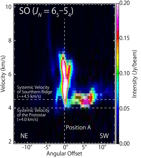
Figure 6: Position-Velocity diagram of the SO ($J_{N}=6_{5}-5_{4}$) line. The position axis is taken along the southern ridge component as shown by the black arrow in Figure 5(d). Angular offset of 0″ shown by the dashed vertical line is taken at Position A. The dashed horizontal lines represent the systemic velocity of the southern ridge ($+4.5$ km s^-1) and that of the protostar ($+4.0$ km s^-1).

To explore the outflow-ridge interaction feature at Position A, we produced a position-velocity (PV) diagram of the SO emission along the southern ridge (Figure 6). The position axis of the PV diagram is taken to pass through the crossing point of the outflow cavity and the southern ridge, as shown in Figure 5(d). The spatially-extended component traces the southern ridge at the systemic velocity of $\sim$$+4.5$ km s^-1. Moreover, a bright component is locally seen at Position A with velocity ranging from $+4.5$ km s^-1 to $+7$ km s^-1, which is red-shifted by 0$-$2.5 km s^-1 from the systemic velocity of the southern ridge ($\sim$$+4.5$ km s^-1) and by 0.5$-$3 km s^-1 from that of the protostar (+4 km s^-1). This strong localized emission can be confirmed in the velocity channel maps of $+5.4$ and $+7.1$ km s^-1 for both the C¹⁸O and SO emissions (Figures 5b, c, e, f). The red-shifted feature is consistent with the previous reports for the eastern outflow lobe by Ceccarelli et al. (2002) or the southeastern one by Bussmann et al. (2007). Among the spectra of the ¹²CO ($J=6-5$) reported by Ceccarelli et al. (2002) (see their Figure 1), the spectrum at 7″ south of the protostar is the one obtained at the position nearest to Position A. The ¹²CO emission peaks at $+6$ km s^-1 and shows a wing there, which was interpreted to trace the outflowing gas (Ceccarelli et al., 2002). This ¹²CO feature, therefore, seems to correspond to the red-shifted component of the SO emission in our Figure 6. Hence, the SO emission at Position A is naturally interpreted as kinematic evidence of the interaction of the outflow with the southern ridge.

Since Position A is located within the north-south extension of the dust continuum emission (Figures 1, 4), one may contemplate whether the warming is due to an additional protostar, perhaps with the larger southern ridge supplying mass. The distribution of the continuum emission around this local peak, however, is broad and not localized, in contrast to that toward the known protostar of Elias 29. Furthermore, the SO emission does not show a clear velocity gradient, expected if gravity is playing a role (e.g. Oya et al., 2022). While the 2MASS Bands H and J data shows an intensity peak at the protostellar position of Elias 29, we do not find any peaks centered at Position A indicating a point-like young stellar object candidate by using Aladin Sky Atlas (Bonnarel et al., 2000). Although we cannot rule out the protostar solution completely, the evidence provides stronger support to a shocked region. In this case, the dust continuum emission has been enhanced due to both an increased density and temperature from the shock; such a feature was reported for a young low-mass protostellar source IRAS 16293$-$2422 by Maureira et al. (2022).

4.2 Temperature Enhancements due to Jet Shock Interactions

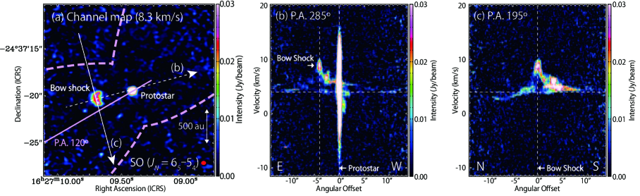
Figure 7: (a) Velocity channel map of the SO ($J_{N}=6_{5}-5_{4}$) line. Velocity of $+8.3$ km s^-1 is red-shifted from the systemic velocity of the protostar ($\sim+4$ km s^-1). Pink dashed and solid lines are the same as those in Figure 5. (b, c) Position-Velocity diagrams of the SO ($J_{N}=6_{5}-5_{4}$) line. Position axes for panels (b, c) are shown by the white dashed and solid arrow in panel (a), respectively. White vertical lines in panels (b, c) represent the protostellar position and Position E, respectively. White horizontal lines in panels (b, c) represent the systemic velocity of the protostar ($+4.0$ km s^-1).

The other clear hot spot, Position E, is on the eastern side of the protostar. It is located inside the southeastern outflow cavity structure, whose central axis has the position angle (P.A.) of $\sim$120°, seen in the C¹⁸O emission (Figure 7a). Furthermore, it is nearly on the central axis of the parabolic shape of the outflow morphology represented by the pink sold line in Figure 7(a), which likely corresponds to the outflow axis. The emission at Position E is evident in the velocity channel map of $+8.3$ km s^-1 as shown in Figure 7(a). This emission is red-shifted by $+4.3$ km s^-1 with respect to the systemic velocity of the protostar ($\sim$$+4$ km s^-1). This observed velocity-shift along the line-of-sight corresponds to a propagating velocity of 24.8 km s^-1 after correcting for projection using the inclination angle of 80° reported by Oya et al. (2019). The direction from this position to the protostar (P.A. 285°) roughly corresponds to the direction of the outflow cavity structure (P.A. 120°) discussed in Section 4.1. Thus, one possible cause for this feature is a bow shock produced by the interaction between the protostellar jet and the ambient gas which has remained undissipated by the outflow.

To verify this picture, we obtained PV diagrams around Position E as shown in Figures 7(b) and (c). The position axes are passing through Position E (Figure 7a). Figure 7(b) shows the PV diagram obtained through Position E and the protostellar position. The compact component concentrated to the protostar is seen as the bright emission with a wide velocity range from $-8$ to $+16$ km s^-1 at the angular offset of 0″. This disk/envelope component was previously analyzed by Oya et al. (2019). In addition to the compact feature, we see several bright knots toward the east of the protostar. The knot with velocity from $+8$ to $+10$ km s^-1 corresponds to the emission at Position E. Taken together, these knots show a velocity gradient from the protostar to Position E; they seem to be accelerated from the systemic velocity of $+4$ km s^-1 at the protostar. Figure 7(c) shows the PV diagram across the outflow lobe passing through Position E. In addition to the widely-extended ($\sim$20″) and slow (from $+2$ to $+6$ km s^-1) component of the outflow structure, we find bright emission associated with a localized ($<$2″) and fast (from $+8$ to $+10$ km s^-1) component. This behavior is naturally expected for a bow shock (e.g. Gustafsson et al., 2010); a bow shock presents the maximum acceleration of the gas at its apex, while the shocked gas is less perturbed away from the axis of the shock. Thus, the bright emission at Position E is interpreted to be a bow shock produced by the narrow jet from the protostar.

It is worth noting that a feature morphologically similar to what we found in Figure 7(b) was found in the SiO emission toward IRDC (infrared dark cloud) G034.77$-$00.55 (Figure 4 by Cosentino et al., 2019) caused by an interaction with the supernova remnant W44, which was interpreted to be a magnetohydrodynamic C-shock. While the shock in G034.77$-$00.55 was suggested to be produced by the deceleration due to the dense material of the IRDC, the shocked gas in Elias 29 seems to accelerate. Thus, we need the shock modeling to examine whether the observed feature is related to a C-shock.

Assuming that the typical observed velocity of the bow shock ($+8$ km s^-1; Figure 7) is comparable to the propagating velocity projected onto the plane of the sky and that the systemic velocity is $+4$ km s^-1, the dynamical time scale of the bow shock is roughly estimated to be

$$t_{\rm dyn}=\frac{d_{\rm shock}}{v_{\rm jet}}\sim\frac{600}{\tan(i)}\ {\rm yr}.$$ (2)

Here, $d_{\rm shock}$ denotes the deprojected distance from the protostar to the bow shock, $v_{\rm jet}$ the deprojected propagating velocity of the jet, and $i$ the inclination angle of the jet axis with respect to the line of sight, where $i$ of 0° corresponds to the pole-on geometry. For instance, $t_{\rm dyn}$, $d_{\rm shock}$, and $v_{\rm jet}$ are obtained to be 110 yr, 560 au, and 23 km s^-1, respectively. Oya et al. (2019) reported the lower limit of 65° for $i$ based on the ellipticity of the continuum emission, and Oya et al. (2022) reported that the rotation motion of the gas associated to the protostar is well reproduced by the Keplerian motion with $i$ of 80°. Then, we assume $i$ of 80° in the above calculation. If we employ the lower (65°) and upper limit (120°) for $i$ discussed in the above literatures, $t_{\rm dyn}$ is calculated to be 280 yr and 350 yr, respectively. If this short time scale of the shock is the case, it would suggest that a mass accretion onto the protostar still occurs in this late Class I source.

4.3 Mass Accretion in the Disk/Envelope System

As described in Sections 4.1 and 4.2, we found a young and energetic outflow/jet emerging from the protostar in this study. This result suggests that significant mass accretion is continuing at least sporadically. Although Elias 29 is a protostellar source at a late Class I stage, Oya et al. (2022) reported that there is still a hint of infall motion of the gas in the compact structure in the vicinity of the protostar in addition to the Keplerian motion.

The relatively large bolometric luminosity ($L_{\rm bol}=13.6$ $L_{\odot}$; Lommen et al., 2008; Miotello et al., 2014) also suggests a moderate accretion rate. When we employ the protostellar mass ($M$) of 0.8 $M_{\odot}$ (Oya et al., 2022), the mass accretion rate ($\dot{M}$) is roughly evaluated to be $1.4\times 10^{-6}$ $M_{\odot}$ yr^-1 by using the following equation given by Palla & Stahler (1991):

$$\dot{M}=\frac{L_{\rm bol}R}{GM},$$ (3)

where $G$ denotes the gravitational constant. We here assume a protostar radius ($R$) 2.5 times the solar radius (Larson, 2003). This mass accretion rate is comparable to the typical value during the main accretion phase (e.g. Hartmann, 2008) and thus larger than that expected at the end of the Class I stage. Such a high accretion rate ($>10^{-6}$ $M_{\odot}$ yr^-1) was also reported for a considerable number of Class I sources by Enoch et al. (2009) (Figure 12 in their paper). These authors concluded that the mass accretion during the Class I stage is episodic, considering the large dispersion in the observed bolometric luminosity.

The disk mass derived from the continuum emission is reported to be $(7.3\pm 0.6)\times 10^{-3}$ $M_{\odot}$ (Artur de la Villarmois et al., 2019). Hence, the disk lifetime should be of the order of $10^{3-4}$ years, if the accretion from the disk component toward the protostar is continuous at the rate evaluated above. This source does not have a massive surrounding envelope which could sustain a continuous accretion at the above rate, as revealed by the lack of such components in our C¹⁸O and CS data. With these considerations, the outflow/jet activities are expected to be sporadic rather than continuous, and the protostar would currently be in a relatively high accretion phase that cannot last for a long time.

The indication of stronger accretion than expected for a late Class I source and the observation of a bow-shaped shock along the jet, within the southeast outflow lobe, suggests that Elias 29 should be investigated for potential accretion variability, as suggested for another luminous Class I source in Perseus by Valdivia-Mena et al. (2022). Non-steady mass assembly during the protostar stage is expected and observed, and can be an important probe of the underlying physical conditions in the disk (Fischer et al., 2023). The JCMT (James Clerk Maxwell Telescope) Transient Survey (Herczeg et al., 2017) has been monitoring Ophiuchus, including Elias 29, for over eight years (Lee et al., 2021; Mairs et al., 2024) at 850 $\mu$m with a 15″ beam and thus far has found no evidence of variability for this source. The same survey, however, has shown that at least 25% of protostars are variable on years-long timescales, with these sources showing both episodic variations (e.g. EC 53; Lee et al., 2020) and burst behavior (e.g. HOPS 373; Yoon et al., 2022). Therefore, continued monitoring of Elias 29 is strongly encouraged.

5 Chemical Characteristics in the Shocked and Warm Environment

5.1 Column Density of SO at the Shock Locations

We evaluated the column density of SO ($N({\rm SO})$) for the six positions shown in Figure 4 under the assumption of the LTE condition with $T_{\rm rot}$ derived in Section 3.2 by using the following equation:

$$N({\rm SO})=U(T_{\rm rot})\frac{3k_{\rm B}W}{8\pi^{3}\nu\ S\mu^{2}}\exp\left(\frac{E_{\rm u}}{k_{\rm B}T_{\rm rot}}\right),$$ (4)

where $U(T_{\rm rot})$ denotes the partition function of SO at the temperature $T_{\rm rot}$, and $k_{\rm B}$ the Boltzmann constant. The line parameters (the frequency $\nu$, $S\mu^{2}$, and $E_{\rm u}$) are summarized in Table Evidence for Jet/Outflow Shocks Heating the Environment Around the Class I Protostellar Source Elias 29: FAUST XXI, while the integrated intensities are in Table Evidence for Jet/Outflow Shocks Heating the Environment Around the Class I Protostellar Source Elias 29: FAUST XXI. Since the integrated intensity $W$ is used, the derived column density is an averaged one over velocity components along the line of sight. The results of the LTE analysis are summarized in Table Evidence for Jet/Outflow Shocks Heating the Environment Around the Class I Protostellar Source Elias 29: FAUST XXI. The obtained column density of SO is similar to each other among Positions B$-$E ($(1.0-1.7)\times 10^{14}$ ${\rm cm}^{-2}$) while it is about 5 times higher at Position A ($8.4\times 10^{14}$ ${\rm cm}^{-2}$). Only the lower limit was obtained at the continuum peak position due to the high opacity of the SO lines. We also conducted a non-LTE analysis for confirmation in Appendix A and found that the column densities derived under the LTE assumption are almost consistent with those derived by the non-LTE analysis, except for Position D with a large error; the difference of the evaluated values are within 20% for Positions A, B, and E between the two analyses, while the evaluated values are different by a factor of 2 for Position C. The error for the non-LTE result is large because the H₂ density is treated as a free parameter as well as the gas kinetic temperature and the column density (see Appendix A).

In principle, it is desirable to derive the SO abundance relative to H₂ by using the H₂ estimated from the C¹⁸O data. However, the line profiles of C¹⁸O at Positions A$-$E are different from those of SO (Figure 3). The C¹⁸O line has a lower critical density than the SO lines and would preferentially trace the different parts along the line of sight. Thus, it is almost impossible to disentangle these components and derive their SO abundances reasonably. Hence, we just discuss the SO column densities in this paper.

SO is often recognized as a shock tracer (e.g. Bachiller & Pérez Gutiérrez, 1997); its abundance in the gas phase is expected to be increased by the sputtering of S atoms and/or SO from dust or ice mantle in shocked regions. The SO column density at the outflow interaction region (Position A) is indeed higher than those at other positions in the southern ridge (Positions B$-$D), which would indicate a sign of shock enhancement. However, the SiO ($J=5-4$) line is undetected toward Position A in our observation, although the SiO emission has been detected and associated with jets and strong shocks in other sources (e.g. Mikami et al., 1992; Bachiller & Pérez Gutiérrez, 1997; Zapata et al., 2009; Feng et al., 2016; Oya et al., 2018a, b; Okoda et al., 2021; Sato et al., 2023) due to the destruction and sputtering of silicate dust grains (Ziurys et al., 1989; Caselli et al., 1997; Schilke et al., 1997). Therefore, the shock at Position A may not be enough strong to destroy or sputter dust grains to liberate SiO into the gas phase. The high column density of SO at Position A may alternatively be due to the high gas column density at that location. In this case, the SO molecules are not originating from dust/ice mantle, but are already in the gas-phase prior to the shock.

For Position E, the SO column density is comparable to the quiescent parts of the southern ridge (Positions B$-$D). Moreover, a lack of SiO emission at Position E is puzzling, considering that the bow shock feature is observed. A detailed relation of the Position E to the outflow is not fully understood and might need further investigation both in observations and modeling.

Oya et al. (2019) previously suggested that the warm environment of Elias 29 prevents C atoms and CO molecules from being adsorbed onto dust grains in the envelope such that this source is deficient in organic molecules. If this is also the case for S atoms, the majority of SO molecules would need to be formed and preserved in the gas-phase. This is likely the case because the desorption temperature of S atoms (1100 K) is less than or comparable to that of C atoms (800 K) and CO molecules (1150 K) according to Kinetic Database for Astrochemist (KIDA; Wakelam et al., 2012, http://kida.obs.u-bordeaux1.fr/), as discussed by Oya et al. (2019).

5.2 Deuterium Fractionation Ratio in the Southern Ridge

The line width of the SO emission is less than 1 km s^-1 at Positions B$-$D as shown in Table Evidence for Jet/Outflow Shocks Heating the Environment Around the Class I Protostellar Source Elias 29: FAUST XXI and Figures 3 and 6. Hence, it is difficult to explain the moderately high rotational temperature of SO (20$-$30 K; Table Evidence for Jet/Outflow Shocks Heating the Environment Around the Class I Protostellar Source Elias 29: FAUST XXI) at these three positions in terms of the recent outflow shock. This situation is different from that at Positions A and E with larger line width, where interactions with the outflow/jet are seen in the velocity structure as discussed in Sections 4.1 and 4.2. Thus, it is important to assess these derived moderately high temperatures in an independent way.

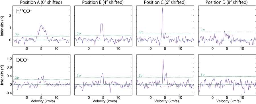
Figure 8: Spectra of the H¹³CO⁺ ($J=3-2$) and DCO⁺ ($J=3-2$) lines. The spectra are obtained for Positions A$-$D (Figure 4). Coordinates of the Positions A$-$D are summarized in Table Evidence for Jet/Outflow Shocks Heating the Environment Around the Class I Protostellar Source Elias 29: FAUST XXI. Each spectrum represents the average over the circular region with a diameter of 1″ centered at each of Positions A$-$D.

As an indicator for the temperature environment, we investigate the deuterium fractionation ratio of HCO⁺ in the southern ridge component. For this purpose, we use the H¹³CO⁺ ($J=3-2$) and DCO⁺ ($J=3-2$) emission, assuming the constant [HCO⁺]/[H¹³CO⁺] ratio of 60 (Lucas & Liszt, 1998). The spectra of H¹³CO⁺ and DCO⁺ emission toward Positions A$-$D are shown in Figure 8, and the line parameters are summarized in Table References. The observed peak intensity of the DCO⁺ spectrum is lower than the noise level at Position D, and thus the 2$\sigma$ noise error is employed as the upper limit. We employ a non-LTE analysis for both the two molecular lines, as we performed for the SO lines (see Appendix A for the details). H₂ is assumed to be the collision partner. Since the collisional cross sections of H¹³CO⁺ are not available, we employ those of HCO⁺ for H¹³CO⁺. The collisional cross sections of HCO⁺ and DCO⁺ are taken from Leiden Atomic and Molecular Database (LAMDA; Schöier et al., 2005), whose original data are reported by Denis-Alpizar et al. (2020). For HCO⁺, the collisional cross sections with para-H₂ and ortho-H₂ are separately listed. We assume the ortho-para ratio of H₂ to be 3 in the analysis. Note that the following results do not change significantly by using an ortho-to-para ratio of 0.

In the $\chi^{2}$ analysis, we use the peak intensities of the H¹³CO⁺ and DCO⁺ intensities listed in Table References. The $\chi^{2}$ values for H¹³CO⁺ and DCO⁺ were summed up to obtain the total $\chi^{2}$ value, which is used to constrain the ranges of the H¹³CO⁺ column density and the [DCO⁺]/[H¹³CO⁺] ratio. In this analysis, the ranges of the gas kinetic temperature and the H₂ number density are assumed to be those derived in the non-LTE analysis for the SO emission (Tables Evidence for Jet/Outflow Shocks Heating the Environment Around the Class I Protostellar Source Elias 29: FAUST XXI).

The estimated [DCO⁺]/[HCO⁺] ratio is summarized in Table References. The [DCO⁺]/[HCO⁺] ratio is below 1.5% including the error for all the positions. These values are relatively low in comparison with those found in typical cold prestellar cores ($\sim$4%; Bacmann et al., 2003). This result indicates a relatively warm condition for the entire southern ridge. This is consistent with the result for the rotational temperature and the gas kinetic temperature derived for SO (Section 3.2).

It is interesting that a moderately high temperature is found even in the quiescent part of the southern ridge. One possible cause for this result is the external illumination by HD 147889, a B-type star at 700″ ($\sim$0.5 pc) northwest of Elias 29. This star is suggested to heat the entire area, and even the whole Ophiuchus molecular cloud. Indeed, Rocha & Pilling (2018) reported that the molecular cloud core of Elias 29 is warmed up to more than 20 K by HD 147889 based on their radiative transfer modeling.

The relatively warm conditions in the southwestern part of the southern ridge without apparent influence of the on-going outflow interaction may also explain the lack of iCOMs and hydrocarbon molecules in Elias 29. If the gas temperature of the parent cloud of Elias 29 were higher than 20 K due to the irradiation from HD 147889, CO molecules and C atoms would not deplete onto dust grains in the prestellar core phase. As a result, iCOMs and CH₄ are not produced efficiently via dust surface reactions (Oya, 2022). This possibility was pointed out by Oya et al. (2019), and it is further strengthened by the temperature structure revealed in this project. Elias 29 is a novel example where the combination of environmental dynamics and radiation triggers peculiar chemistry. This situation is possibly similar to that of the photodissociation region (PDR) R CrA IRS7B (Watanabe et al., 2012; Lindberg et al., 2015) where the abundance of iCOMs has been found to be unexpectedly deficient in a single dish survey. On the other hand, the difference is the abundance of the CCH emission, which is known to be enhanced by the PDR (photodissociation region). The fractional abundance of CCH to H₂ is reported to be $(5.3\pm 1.5)\times 10^{-9}$ in R CrA IRS7B with the gas temperature assumed to be 20 K (Watanabe et al., 2012), while its upper limit is $(1.3-9.0)\times 10^{-11}$ in Elias 29 with the gas and dust temperatures assumed to be from 50 to 150 K (Oya et al., 2019). This large difference in the fractional abundance of CCH by the two order of magnitude implies that the PDR chemistry is not working in Elias 29 probably due to heavier attenuation of the far UV photons dissociating CO.

6 Summary

In order to characterize the protostellar activity of the late Class I source Elias 29, we observed lines of SO, ³⁴SO, C¹⁸O, CS, SiO, H¹³CO⁺, and DCO⁺ at a spatial resolution of 70 au (0$\farcs$5). This investigation is part of the ALMA large program FAUST. Our major findings are summarized below.

• We delineated the temperature distribution by using two transitions of SO and one of ³⁴SO. We obtained a two-dimensional map of the rotational temperature of SO, using LTE assumptions, and found two hot spots with the rotational temperature of $53^{+25}_{-15}$ and $72^{+66}_{-29}$ K in addition to the hot component associated with the protostar. These locally high temperatures were confirmed with a non-LTE analysis.

• The local increase of the temperature at the northeastern tip of the southern ridge component is likely attributed to interaction with the southeast outflow lobe. The other local temperature increase is interpreted as the result of a bow shock produced by the jet. It is interesting that Elias 29 still has significant outflow/jet activity at least sporadically in spite of its classification as a late-type Class I.

• It is likely that significant mass accretion from disk to protostar is still occurring at least sporadically, considering the energetic activity of the outflow/jet in Elias 29 observed in this project, the hint of the infall motion in its disk/envelope system previously suggested, and its relatively large luminosity. The mass accretion rate is roughly evaluated to be $1.4\times 10^{-6}$ $M_{\odot}$ yr^-1, which sounds high for the late Class I stage of this source. Since the outer envelope has already been consumed/dissipated, as demonstrated by the lack of the C¹⁸O emission associated around the protostar, we are likely witnessing the near end of the mass accretion phase.

• We evaluated the SO column density at the five positions (Positions A$-$E). Although the SO column density at the outflow-ridge interaction region (Position A) is found to be higher by a factor of 5 than in the quiescent part of the southern ridge (Positions B$-$D), the SiO emission is not detected there. This result may indicate that the shock is not strong enough to destruct or sputter the silicate dust grains at Position A. In spite of the bow-shock feature at Position E, the SiO emission is not detected there either, and the SO column density is comparable to those at Positions B$-$D. The origin of these results at Position E is still puzzling; further observational and modeling efforts are necessary.

• Even the quiescent parts of the southern ridge at distances ranging from 500 to 1000 au away from the protostar are found to be moderately warm (20$-$30 K). This warm condition is consistent with our estimated relatively low deuterium fractionation (1% or less) in HCO⁺. The B-type star HD 147889, which is 700″ away from Elias 29, would likely have kept the parent cloud of Elias 29 warm. Such a warm environment for the entire lifetime of this source could be the cause for its peculiar chemical characteristics including a deficiency of iCOMs and hydrocarbon molecules.

Appendix A Non-LTE Analysis for SO

To confirm whether the results obtained by the LTE (local thermodynamic equilibrium) analysis for SO (Figure 4b; Section 3.2) is reasonable, we conduct a non-LTE analysis. The non-LTE analysis is performed for five picked-up positions (A through E), unlike the pixel-based method for the calculation of the rotational temperature of SO.

We use the ³⁴SO ($J_{N}=5_{6}-4_{5}$) line data in the non-LTE analysis in addition to the two SO ($J_{N}=6_{5}-5_{4}$, $J_{N}=6_{6}-5_{5}$) lines for accurate determination of the gas kinetic temperature. Figure 3 shows the spectra of these three lines at Positions A$-$E. Although the ³⁴SO emission is much fainter than the SO emission, it is detected toward Positions A$-$D with the S/N ratio higher than 6. Meanwhile, the detection of the ³⁴SO emission is marginal at Position E, where the S/N ratio is 3.6. The parameters of the spectra are summarized in Table Evidence for Jet/Outflow Shocks Heating the Environment Around the Class I Protostellar Source Elias 29: FAUST XXI. The ³⁴SO line is frequency-diluted, since it is observed with a coarse-resolution backend (1.129 MHz). Hence, its peak intensity at each position is derived from the integrated intensity divided by the averaged line width of the two SO lines.

We conduct the non-LTE modeling and constrain the gas kinetic temperature, the SO column density, and the H₂ number density by the $\chi^{2}$ method. We employed the escape probability for a static, spherically symmetric, and homogeneous medium (Osterbrock & Ferland, 2006; van der Tak et al., 2007). We employ the energy levels, the Einstein A coefficients, and the state-to-state collisional rates of SO by Price et al. (2021). The energy levels and the Einstein A coefficients of ³⁴SO are taken from CDMS (Müller et al., 2005; Endres et al., 2016). We employ H₂ as the collision partner. Since the collisional rates of ³⁴SO are not available, we employ those of SO as substitutes without any corrections. We assume the ratio of $N\left({}^{32}{\rm SO}\right)/N\left({}^{34}{\rm SO}\right)$ to be 19 in this calculation (Lucas & Liszt, 1998).

In the $\chi^{2}$ analysis, the SO and ³⁴SO data are treated simultaneously in the $\chi^{2}$ analysis. Thus, the $\chi^{2}$ value is calculated by the following equation;

$$\chi^{2}=\Sigma_{i}\left(\frac{T_{i}^{\rm obs}-T_{i}^{\rm calc}}{\sigma_{i}^{2}}\right)^{2},$$ (A1)

where the summation is taken over the two SO and one ³⁴SO lines. $T_{i}^{\rm obs}$ and $T_{i}^{\rm calc}$ denote the observed and calculated peak temperatures. $\sigma_{i}$ stands for the error of the observed temperature which is calculated from the two times the root-mean-square (rms) noise level of each spectrum and 10% of the intensity calibration error. $T_{i}^{\rm obs}$ and its rms are summarized in Table Evidence for Jet/Outflow Shocks Heating the Environment Around the Class I Protostellar Source Elias 29: FAUST XXI.

In the analysis, we scan wide ranges of parameter values to find the best-fit parameter values: every 2.5 K from 30 to 117.5 K for the gas kinetic temperature, every $0.25\times 10^{14}$ ${\rm cm}^{-2}$ from 8 to $13.75\times 10^{14}$ ${\rm cm}^{-2}$ for the SO column density, and every 1.5 times from $3\times 10^{5}$ to $5.05\times 10^{9}$ ${\rm cm}^{-3}$ for the H₂ number density. The results are summarized in Table Evidence for Jet/Outflow Shocks Heating the Environment Around the Class I Protostellar Source Elias 29: FAUST XXI. The error values denote the range of the parameter value which corresponds to the above intensity error.

At Position A, the interaction position of the outflow and the southern ridge component, the gas kinetic temperature is derived to be $55^{+39}_{-14}$ K. The relatively high temperature derived for Position A indicates that the shock heating is indeed occurring there, as discussed in Section 4.1. The gas kinetic temperatures are evaluated to be $>23$ K, $26^{+15}_{-3}$, and $>16$ K at Positions B, C, and D in the southern ridge, respectively. Although only the lower limits are obtained for Positions B and D, the gas kinetic temperature tends to decrease as leaving from Position A, and also from the protostar, along the southern ridge; however, it is still higher than 16 K at Position D, which is the end of the southern ridge.

Only the lower limit is available for the gas kinetic temperature at Position E. Since the ³⁴SO emission is marginally seen, the constraint on the parameters is rather loose (Table Evidence for Jet/Outflow Shocks Heating the Environment Around the Class I Protostellar Source Elias 29: FAUST XXI). Nevertheless, the high temperature ($>$56 K) condition is indeed confirmed, as suggested by the rotational temperature of SO (Figure 4). This result supports the local heating occurring at Position E, as well as the result for Position A; the heating mechanism is likely attributed to the bow shock at Position E, as discussed in Section 4.2.

List of the Observed Lines^a Molecule Frequency (GHz) $S\mu^{2}$ (D²) $E_{\rm u}$ (K) Beam size^b rms (mJy beam^-1) C¹⁸O ($J=2-1$) 219.5603541 0.0244 16 $0\farcs 531\times 0\farcs 438$ (P.A. $-89.\!\!\arcdeg 463$) 1.8 SO ($J_{N}=6_{5}-5_{4}$) 219.949442 14.0 35 $0\farcs 528\times 0\farcs 435$ (P.A. $89.\!\!\arcdeg 739$) 2.3^c SO ($J_{N}=6_{6}-5_{5}$) 258.2558259 13.7 57 $0\farcs 573\times 0\farcs 451$ (P.A. $-79.\!\!\arcdeg 952$) 2.5^{c 34}SO ($J_{N}=5_{6}-4_{5}$) 246.66347 11.4 50 $0\farcs 518\times 0\farcs 392$ (P.A. $-73.\!\!\arcdeg 648$) 1.3 CS ($J=5-4$) 244.9355565 19.2 35 $0\farcs 523\times 0\farcs 402$ (P.A. $-73.\!\!\arcdeg 669$) 1.8 SiO ($J=5-4$) 217.1049190 48.0 31 $0\farcs 537\times 0\farcs 439$ (P.A. $-88.\!\!\arcdeg 865$) 1.7 H¹³CO⁺ ($J=3-2$) 260.255339 45.6 25 $0\farcs 497\times 0\farcs 381$ (P.A. $-73.\!\!\arcdeg 099$) 2.8 DCO⁺ ($J=3-2$) 216.1125822 45.6 21 $0\farcs 540\times 0\farcs 442$ (P.A. $-88.\!\!\arcdeg 636$) 2.3

• Taken from CDMS (Müller et al., 2005; Endres et al., 2016).

• Synthesized beam.

• Root-mean-square noise of the data with the beam size of $0\farcs 6\times 0\farcs 6$.

Observation Parameters Configuration Date $\rm{T_{\rm target}}$ $\rm{N_{Antennas}}$ Baseline MRS^a Calibrator (min) (meter) (arcsec) Phase Bandpass Flux Setup 1 C43-4 2018 Dec 2 29.35 43 15.1$-$783.5 5.7 J1625$-$2527 J1427$-$4206 J1427$-$4206 C43-4 2019 May 4 29.35 40 15.1$-$740.4 5.5 J1626$-$2951 J1427$-$4206 J1427$-$4206 C43-4 2020 Mar 16 29.33 44 15.2$-$968.7 5.4 J1626$-$2951 J1517$-$2422 J1517$-$2422 C43-1 2019 Jan 21 10.12 48 15.0$-$313.7 11.3 J1625$-$2527 J1517$-$2422 J1517$-$2422 ACA 2018 Nov 18 34.83 10 8.9$-$44.7 30.3 J1625$-$2527 J1256$-$0547 J1256$-$0547 ACA 2018 Nov 22 34.78 12 8.9$-$48.9 30.3 J1625$-$2527 J1337$-$1257 J1337$-$1257 Setup 2 C43-4 2018 Dec 1 20.73 43 15.1$-$951.7 5.3 J1625$-$2527 J1427$-$4206 J1427$-$4206 C43-4 2019 Apr 17 20.75 46 15.1$-$740.4 5.6 J1650$-$2943 J1517$-$2422 J1517$-$2422 C43-4 2019 Oct 11 20.72 43 15.1$-$783.5 5.5 J1626$-$2951 J1427$-$4206 J1427$-$4206 C43-1 2019 Jan 21 7.10 48 15.0$-$313.7 10.0 J1625$-$2527 J1517$-$2422 J1517$-$2422 ACA 2018 Oct 25 49.43 11 8.9$-$48.9 26.9 J1700$-$2610 J1924$-$2914 J1924$-$2914

• Maximum recoverable scale.

Coordinates of the Positions A-E and C.P. Position Right Ascension (ICRS) Declination (ICRS) Note A $16^{\rm h}27^{\rm m}09.\!\!^{\rm s}476$ $-24\arcdeg 37\arcmin 23\farcs 533$ Outflow interaction in the southern ridge B $16^{\rm h}27^{\rm m}09.\!\!^{\rm s}251$ $-24\arcdeg 37\arcmin 26\farcs 104$ 4″ from Position A along the southern ridge C $16^{\rm h}27^{\rm m}09.\!\!^{\rm s}139$ $-24\arcdeg 37\arcmin 27\farcs 390$ 6″ from Position A along the southern ridge D $16^{\rm h}27^{\rm m}09.\!\!^{\rm s}027$ $-24\arcdeg 37\arcmin 28\farcs 675$ 8″ from Position A along the southern ridge E $16^{\rm h}27^{\rm m}09.\!\!^{\rm s}692$ $-24\arcdeg 37\arcmin 20\farcs 043$ Bow shock by the jet C.P. $16^{\rm h}27^{\rm m}09.\!\!^{\rm s}41737$ $-24\arcdeg 37\arcmin 19\farcs 3104$ 1.2 mm continuum peak position

• Spectra of the molecular lines are obtained as the averages over the circular region with a diameter of 1″ centered at each of Positions A$-$D. Meanwhile, those with the original synthesized beam is employed for Positions E and C.P.

Parameters of the SO ($J_{N}=6_{5}-5_{4}$, $J_{N}=6_{6}-5_{5}$) and ³⁴SO ($J_{N}=5_{6}-4_{5}$) Emissions Position Line $T_{\rm peak}$/K ^a $V_{\rm LSR}$/ km s^-1 b $\Delta v$/ km s^-1 c $W$/K km s^{-1 d} A SO ($J_{N}=6_{5}-5_{4}$) 24.3(24) 5.24 2.32 56.6(57) SO ($J_{N}=6_{6}-5_{5}$) 20.2(20) 5.02 2.15 43.4(43) ³⁴SO ($J_{N}=5_{6}-4_{5}$) 1.19(13) $-$ $-$ $2.67(13)$ B SO ($J_{N}=6_{5}-5_{4}$) 16.57(17) 4.56 0.60 11.3(12) SO ($J_{N}=6_{6}-5_{5}$) 9.92(99) 4.56 0.53 6.1(7) ³⁴SO ($J_{N}=5_{6}-4_{5}$) 0.48(58) $-$ $-$ $0.27(16)$ C SO ($J_{N}=6_{5}-5_{4}$) 18.5(19) 4.42 0.64 12.9(14) SO ($J_{N}=6_{6}-5_{5}$) 13.5(14) 4.33 0.53 7.9(9) ³⁴SO ($J_{N}=5_{6}-4_{5}$) 1.26(59) $-$ $-$ $0.73(17)$ D SO ($J_{N}=6_{5}-5_{4}$) 12.0(12) 4.56 0.76 10.4(11) SO ($J_{N}=6_{6}-5_{5}$) 6.53(65) 4.67 0.62 4.5(7) ³⁴SO ($J_{N}=5_{6}-4_{5}$) 0.83(65) $-$ $-$ $0.6(2)$ E SO ($J_{N}=6_{5}-5_{4}$) 3.8(5) 8.50(8) 1.79(18) 6.1(7) SO ($J_{N}=6_{6}-5_{5}$) 3.3(4) 8.42(6) 1.70(14) 5.2(6) ³⁴SO ($J_{N}=5_{6}-4_{5}$) 0.26(14) 10.0(5) 1.75(fixed) 0.4(2) C.P. SO ($J_{N}=6_{5}-5_{4}$) $-$ $-$ $-$ 201(20) SO ($J_{N}=6_{6}-5_{5}$) $-$ $-$ $-$ 230(23) ³⁴SO ($J_{N}=5_{6}-4_{5}$) $-$ $-$ $-$ 21(3)

• The numbers in parentheses represent the error in units of the last significant digits.

• Peak intensity of the observed line profiles for Positions A$-$D. The error is evaluated from twice the rms noise of each spectrum and the 10% intensity calibration error, where the latter contribution dominates the total error. Since the ³⁴SO emission is frequency-diluted due to a coarse-resolution backend, its peak intensity is derived from the integrated intensity divided by the averaged line width of the two SO lines (see Appendix A). For Position E, the peak intensity is derived by the Gaussian fitting.

• LSR velocity of the intensity peak of the observed line profiles for Positions A$-$D. For Position E, the Gaussian fitted value is employed.

• FWHM of the line width. The Gaussian fitted value is employed. Although the spectrum is not well fitted to define the peak intensity due to the asymmetric line shape for Positions A$-$D, the line width obtained by the fit is approximately employed as the best effort.

• Observed integrated intensity from 0.0 to $+10.0$ km s^-1 for Positions A$-$D, that from $+7.0$ to $+10.5$ km s^-1 for Position E, and that from $-15.0$ to $+23.0$ km s^-1 for the continuum peak (C.P.) position.

Column Density and Rotational Temperature of SO at Representative Positions LTE^a non-LTE^b Position $N({\rm SO})/10^{14}$ ${\rm cm}^{-2}$ $T_{\rm rot}$ (K) $N({\rm SO})/10^{14}{\rm cm}^{-2}$ $T_{\rm kin}$ (K) $n({\rm H}_{2})/10^{6}$ ${\rm cm}^{-3}$ A $8.4^{+1.2}_{-0.6}$ $53^{+25}_{-15}$ $10.7^{+1.2}_{-1.7}$ $55^{+39}_{-14}$ $>1.2$ B $1.5^{+0.2}_{-0.2}$ $28^{+7}_{-5}$ $1.3^{+2.6}_{-0.2}$ $>23$ $>0.2$ C $1.7^{+0.2}_{-0.1}$ $34^{+10}_{-7}$ $3.6^{+3.1}_{-1.6}$ $26^{+15}_{-3}$ $>0.4$ D $1.5^{+0.3}_{-0.2}$ $22^{+5}_{-4}$ $7.3^{+11.0}_{-6.3}$ $>16$ $>0.11$ E $1.0^{+0.5}_{-0.2}$ $72^{+66}_{-29}$ $1.2^{+0.8}_{-0.4}$ $>56$ $>0.4$ C.P. $>71$ $>192$ $-$ $-$ $-$

• Values are derived under the assumptions of the LTE and optically thin conditions. See Sections 3.2 and 5.1. The observed integrated intensities are summarized in Table Evidence for Jet/Outflow Shocks Heating the Environment Around the Class I Protostellar Source Elias 29: FAUST XXI. The error is derived from the 2$\sigma$ noise error in the integrated intensities and the intensity calibration error of 10%.

• Values are derived by the non-LTE analyses. See Appendix A for the details. The observed peak intensities are summarized in Table Evidence for Jet/Outflow Shocks Heating the Environment Around the Class I Protostellar Source Elias 29: FAUST XXI. The error is derived from the 2$\sigma$ noise error in the intensities and the intensity calibration error of 10%.

Parameters of the H¹³CO⁺ and DCO⁺ Spectra in the Southern Ridge Position Line $T_{\rm peak}$/K ^a $V_{\rm LSR}$/km s^-1 b $\Delta v$/km s^-1 c A H¹³CO⁺ ($J=3-2$) 1.15(14) 5.14(8) 2.46(20) DCO⁺ ($J=3-2$) 0.29(7) 5.3(2) 1.9(5) B H¹³CO⁺ ($J=3-2$) 1.56(22) 4.41(4) 0.84(10) DCO⁺ ($J=3-2$) 0.56(17) 4.60(10) 0.77(24) C H¹³CO⁺ ($J=3-2$) 2.7(5) 4.03(2) 0.31(6) DCO⁺ ($J=3-2$) 1.2(4) 4.31(8) 0.37(20) D H¹³CO⁺ ($J=3-2$) 0.51(19) 4.7(2) 1.6(6) DCO⁺ ($J=3-2$) $<0.20$^d - -

• The numbers in parentheses represent the error in units of the last significant digits, which is derived from the 2$\sigma$ noise error and the intensity calibration error of 10%.

• Peak intensity derived by the Gaussian fitting for each spectrum.

• LSR velocity at the intensity peak derived by the Gaussian fitting for each spectrum.

• FWHM of the line width derived by the Gaussian fitting for each spectrum.

• Since the DCO⁺ emission is too weak to perform the Gaussian fitting at Position D, we employ the 2$\sigma$ value as the upper limit for $T_{\rm peak}$.

Deuterium Fractionation Ratio in the Southern Ridge Position $N$(H¹³CO⁺)/$10^{11}$ cm^-2 $N$(DCO⁺)/$N$(H¹³CO⁺) $N$(DCO⁺)/$N$(HCO⁺) A $12^{+11}_{-3}$ $0.3^{+0.2}_{-0.1}$ $0.005^{+0.003}_{-0.002}$ B $7^{+25}_{-2}$ $0.4^{+0.2}_{-0.3}$ $0.007^{+0.003}_{-0.005}$ C $5^{+10}_{-1}$ $0.5^{+0.3}_{-0.4}$ $0.009^{+0.005}_{-0.006}$ D $6^{+57}_{-3}$ $<0.94$ $<0.015$

• The temperature and density ranges are assumed to be equal to that derived from the non-LTE analysis of the SO lines (Table Evidence for Jet/Outflow Shocks Heating the Environment Around the Class I Protostellar Source Elias 29: FAUST XXI).

References

- Andrews et al. (2018) Andrews, S. M., Huang, J., Pérez, L. M., et al. 2018, ApJ, 869, L41. doi:10.3847/2041-8213/aaf741
- Arce & Sargent (2006) Arce, H. G. & Sargent, A. I. 2006, ApJ, 646, 1070.
- Arce et al. (2008) Arce, H. G., Santiago-Garcia, J., Jørgensen, J. K. et al., 2008, ApJ, 681, L21.
- Artur de la Villarmois et al. (2019) Artur de la Villarmois, E., Jørgensen, J. K., Kristensen, L. E., et al. 2019, A&A, 626, A71.
- Artur de la Villarmois et al. (2022) Artur de la Villarmois, E., Guzmán, V. V., Jørgensen, J. K., et al. 2022, A&A, 667, A20. doi:10.1051/0004-6361/202244312
- Bachiller (1996) Bachiller, R. 1996, ARA&A, 34, 111.
- Bachiller et al. (2001) Bachiller, R., Pérez Gutiérrez, M., Kumar, M. S. N., et al. 2001, A&A, 372, 899. doi:10.1051/0004-6361:20010519
- Bachiller & Pérez Gutiérrez (1997) Bachiller, R. & Pérez Gutiérrez, M. 1997, ApJ, 487, L93.
- Bacmann et al. (2003) Bacmann, A., Lefloch, B., Ceccarelli, C., et al. 2003, ApJ, 585, L55.
- Bally (2016) Bally, J. 2016, ARA&A, 54, 491.
- Baraffe & Chabrier (2010) Baraffe, I. & Chabrier, G. 2010, A&A, 521, A44. doi:10.1051/0004-6361/201014979
- Bianchi et al. (2022) Bianchi, E., Ceccarelli, C., Codella, C., et al. 2022, A&A, 662, A103. doi:10.1051/0004-6361/202141893
- Bianchi et al. (2023) Bianchi, E., López-Sepulcre, A., Ceccarelli, C., et al. 2023, Faraday Discussions, 245, 164. doi:10.1039/D3FD00018D
- Blandford & Payne (1982) Blandford, R. D. & Payne, D. G. 1982, MNRAS, 199, 883.
- Bonnarel et al. (2000) Bonnarel, F., Fernique, P., Bienaymé, O., et al. 2000, A&AS, 143, 33. doi:10.1051/aas:2000331
- Bussmann et al. (2007) Bussmann, R. S., Wong, T. W., Hedden, A. S., et al. 2007, ApJ, 657, L33.
- CASA Team et al. (2022) CASA Team, Bean, B., Bhatnagar, S., et al. 2022, PASP, 134, 114501. doi:10.1088/1538-3873/ac9642
- Caselli et al. (1997) Caselli, P., Hartquist, T. W., & Havnes, O. 1997, A&A, 322, 296
- Ceccarelli et al. (2002) Ceccarelli, C., Boogert, A. C. A., Tielens, A. G. G. M., et al. 2002, A&A, 395, 863.
- Ceccarelli et al. (2010) Ceccarelli, C., Bacmann, A., Boogert, A., et al. 2010, A&A, 521, L22. doi:10.1051/0004-6361/201015081
- Ceccarelli et al. (2017) Ceccarelli, C., Caselli, P., Fontani, F., et al. 2017, ApJ, 850, 176. doi:10.3847/1538-4357/aa961d
- Codella et al. (2010) Codella, C., Lefloch, B., Ceccarelli, C., et al. 2010, A&A, 518, L112.
- Codella et al. (2021a) Codella, C., Bianchi, E., Podio, L., et al. 2021, A&A, 654, A52. doi:10.1051/0004-6361/202141485
- Codella et al. (2021b) Codella, C., Ceccarelli, C., Chandler, C., et al. 2021, Frontiers in Astronomy and Space Sciences, 8, 227.
- Codella et al. (2024) Codella, C., Podio, L., De Simone, M., et al. 2024, MNRAS, 528, 7383. doi:10.1093/mnras/stae472
- Cosentino et al. (2019) Cosentino, G., Jiménez-Serra, I., Caselli, P., et al. 2019, ApJ, 881, L42. doi:10.3847/2041-8213/ab38c5
- Curtis et al. (2010) Curtis, E. I., Richer, J. S., Swift, J. J., et al. 2010, MNRAS, 408, 1516.
- Denis-Alpizar et al. (2020) Denis-Alpizar, O., Stoecklin, T., Dutrey, A., et al. 2020, MNRAS, 497, 4276. doi:10.1093/mnras/staa2308
- Endres et al. (2016) Endres, C. P., Schlemmer, S., Schilke, P., et al. 2016, Journal of Molecular Spectroscopy, 327, 95.
- Enoch et al. (2009) Enoch, M. L., Evans, N. J., Sargent, A. I., et al. 2009, ApJ, 692, 973. doi:10.1088/0004-637X/692/2/973
- Feng et al. (2016) Feng, S., Beuther, H., Zhang, Q., et al. 2016, ApJ, 828, 100. doi:10.3847/0004-637X/828/2/100
- Fischer et al. (2023) Fischer, W. J., Hillenbrand, L. A., Herczeg, G. J., et al. 2023, Protostars and Planets VII, 534, 355. doi:10.48550/arXiv.2203.11257
- Gustafsson et al. (2010) Gustafsson, M., Ravkilde, T., Kristensen, L. E., et al. 2010, A&A, 513, A5. doi:10.1051/0004-6361/200912977
- Hartmann (2008) Hartmann, L. 2008, Accretion Processes in Star Formation, by Lee Hartmann, Cambridge, UK: Cambridge University Press, 2008
- Hatchell et al. (2007) Hatchell, J., Fuller, G. A., & Richer, J. S. 2007, A&A, 472, 187.
- Herczeg et al. (2017) Herczeg, G. J., Johnstone, D., Mairs, S., et al. 2017, ApJ, 849, 43. doi:10.3847/1538-4357/aa8b62
- Hirota et al. (2017) Hirota, T., Machida, M. N., Matsushita, Y., et al. 2017, Nature Astronomy, 1, 0146.
- Imai et al. (2016) Imai, M., Sakai, N., Oya, Y., et al. 2016, ApJ, 830, L37. doi:10.3847/2041-8205/830/2/L37
- Imai et al. (2022) Imai, M., Oya, Y., Svoboda, B., et al. 2022, ApJ, 934, 70.
- Larson (2003) Larson, R. B., 2003, Reports on Progress in Physics, 66, 1651.
- Lee et al. (2000) Lee, C.-F., Mundy, L. G., Reipurth, B., et al. 2000, ApJ, 542, 925.
- Lee et al. (2020) Lee, Y.-H., Johnstone, D., Lee, J.-E., et al. 2020, ApJ, 903, 5. doi:10.3847/1538-4357/abb6fe
- Lee et al. (2021) Lee, Y.-H., Johnstone, D., Lee, J.-E., et al. 2021, ApJ, 920, 119. doi:10.3847/1538-4357/ac1679
- Le Gal et al. (2020) Le Gal, R., Öberg, K. I., Huang, J., et al. 2020, ApJ, 898, 131. doi:10.3847/1538-4357/ab9ebf
- Lindberg et al. (2015) Lindberg, J. E., Jørgensen, J. K., Watanabe, Y., et al. 2015, A&A, 584, A28. doi:10.1051/0004-6361/201526222
- Lommen et al. (2008) Lommen, D., Jørgensen, J. K., van Dishoeck, E. F., et al. 2008, A&A, 481, 141.
- Lucas & Liszt (1998) Lucas, R. & Liszt, H. 1998, A&A, 337, 246
- Machida et al. (2008) Machida, M. N., Inutsuka, S.-. ichiro ., & Matsumoto, T. 2008, ApJ, 676, 1088.
- Machida & Basu (2019) Machida, M. N. & Basu, S. 2019, ApJ, 876, 149.
- Machida & Hosokawa (2013) Machida, M. N. & Hosokawa, T. 2013, MNRAS, 431, 1719. doi:10.1093/mnras/stt291
- Mairs et al. (2024) Mairs, S., Lee, S., Johnstone, D., et al. 2024, ApJ, 966, 215. doi:10.3847/1538-4357/ad35b6
- Matsushita et al. (2019) Matsushita, Y., Takahashi, S., Machida, M. N., et al. 2019, ApJ, 871, 221. doi:10.3847/1538-4357/aaf1b6
- Maureira et al. (2022) Maureira, M. J., Gong, M., Pineda, J. E., et al. 2022, ApJ, 941, L23. doi:10.3847/2041-8213/aca53a
- McMullin et al. (2007) McMullin, J. P., Waters, B., Schiebel, D., et al. 2007, Astronomical Data Analysis Software and Systems XVI, 376, 127
- Mikami et al. (1992) Mikami, H., Umemoto, T., Yamamoto, S., et al. 1992, ApJ, 392, L87.
- Miotello et al. (2014) Miotello, A., Testi, L., Lodato, G., et al. 2014, A&A, 567, A32. doi:10.1051/0004-6361/201322945
- Müller et al. (2005) Müller, H. S. P., Schlöder, F., Stutzki, J., et al. 2005, Journal of Molecular Structure, 742, 215. doi:10.1016/j.molstruc.2005.01.027
- Nakamura et al. (2011a) Nakamura, F., Sugitani, K., Shimajiri, Y., et al. 2011, ApJ, 737, 56.
- Nakamura et al. (2011b) Nakamura, F., Kamada, Y., Kamazaki, T., et al. 2011, ApJ, 726, 46.
- Nakamura & Li (2014) Nakamura, F. & Li, Z.-Y. 2014, ApJ, 783, 115.
- Öberg et al. (2021) Öberg, K. I., Guzmán, V. V., Walsh, C., et al. 2021, ApJS, 257, 1. doi:10.3847/1538-4365/ac1432
- Offner & Chaban (2017) Offner, S. S. R. & Chaban, J. 2017, ApJ, 847, 104.
- Ohashi et al. (2014) Ohashi, N., Saigo, K., Aso, Y., et al. 2014, ApJ, 796, 131. doi:10.1088/0004-637X/796/2/131
- Ohashi et al. (2022) Ohashi, S., Claudio, C., Sakai, N., et al. 2022, ApJ, 927, 54.
- Okoda et al. (2021) Okoda, Y., Oya, Y., Francis, L., et al. 2021, ApJ, 910, 11.
- Omura et al. (2024) Omura, M., Tokuda, K., & Machida, M. N. 2024, ApJ, 963, 72. doi:10.3847/1538-4357/ad19ce
- Ortiz-León et al. (2017) Ortiz-León, G. N., Loinard, L., Kounkel, M. A., et al. 2017, ApJ, 834, 141.
- Osterbrock & Ferland (2006) Osterbrock, D. E. & Ferland, G. J. 2006, Astrophysics of gaseous nebulae and active galactic nuclei, 2nd. ed. by D.E. Osterbrock and G.J. Ferland. Sausalito, CA: University Science Books, 2006
- Oya et al. (2014) Oya, Y., Sakai, N., Sakai, T., et al. (2014), ApJ, 795, 152.
- Oya et al. (2015) Oya, Y., Sakai, N., Lefloch, B., et al. 2015, ApJ, 812, 59. doi:10.1088/0004-637X/812/1/59
- Oya et al. (2016) Oya, Y., Sakai, N., López-Sepulcre, A., et al. 2016, ApJ, 824, 88. doi:10.3847/0004-637X/824/2/88
- Oya et al. (2017) Oya, Y., Sakai, N., Watanabe, Y., et al. 2017, ApJ, 837, 174. doi:10.3847/1538-4357/aa6300
- Oya et al. (2018a) Oya, Y., Sakai, N., Watanabe, Y., et al. 2018, ApJ, 863, 72.
- Oya et al. (2018b) Oya, Y., Moriwaki, K., Onishi, S., et al. 2018, ApJ, 854, 96. doi:10.3847/1538-4357/aaa6c7
- Oya et al. (2019) Oya, Y., López-Sepulcre, A., Sakai, N., et al. 2019, ApJ, 881, 112.
- Oya & Yamamoto (2020) Oya, Y. & Yamamoto, S. 2020, ApJ, 904, 185. doi:10.3847/1538-4357/abbe14
- Oya et al. (2021) Oya, Y., Watanabe, Y., López-Sepulcre, A., et al. 2021, ApJ, 921, 12.
- Oya et al. (2022) Oya, Y., Kibukawa, H., Miyake, S., et al. 2022, PASP, 134, 094301.
- Oya (2022) Oya, Y. 2022, “A Few Tens au Scale Physical and Chemical Structures Around Young Low-Mass Protostars”, Springer Nature Singapore Pte Ltd. 2022, doi:10.1007/978-981-19-1708-0
- Oya et al. (in prep.) Oya, Y., Ceccarelli C., Chandler C., Codella C., et al., Interstellar Matter and Local Universe, in prep.
- Palla & Stahler (1991) Palla, F. & Stahler, S. W. 1991, ApJ, 375, 288.
- Pineau des Forets et al. (1997) Pineau des Forets, G., Flower, D. R., & Chieze, J.-P. 1997, Herbig-Haro Flows and the Birth of Stars, 182, 199
- Podio et al. (2017) Podio, L., Codella, C., Lefloch, B., et al. 2017, MNRAS, 470, L16.
- Price et al. (2021) Price, T. J., Forrey, R. C., Yang, B., et al. 2021, J. Chem. Phys., 154, 034301. doi:10.1063/5.0036964
- Rocha & Pilling (2018) Rocha, W. R. M. & Pilling, S. 2018, MNRAS, 478, 5190.
- Sato et al. (2023) Sato, A., Tokuda, K., Machida, M. N., et al. 2023, ApJ, 958, 102. doi:10.3847/1538-4357/ad0132
- Schilke et al. (1997) Schilke, P., Walmsley, C. M., Pineau des Forets, G., et al. 1997, A&A, 321, 293
- Schöier et al. (2005) Schöier, F. L., van der Tak, F. F. S., van Dishoeck, E. F., et al. 2005, A&A, 432, 369.
- Sekimoto et al. (1997) Sekimoto, Y., Tatematsu, K., Umemoto, T., et al. 1997, ApJ, 489, L63.
- Shingledecker et al. (2020) Shingledecker, C. N., Lamberts, T., Laas, J. C., et al. 2020, ApJ, 888, 52. doi:10.3847/1538-4357/ab5360
- Sugimura et al. (2011) Sugimura, M, Yamaguchi, T., Sakai, T., et al. 2011, PASJ, 63, 459.
- Tanious et al. (2024) Tanious, M., Le Gal, R., Neri, R., et al. 2024, A&A, 687, A92. doi:10.1051/0004-6361/202348785
- Tokuda et al. (2014) Tokuda, K., Onishi, T., Saigo, K., et al. 2014, ApJ, 789, L4. doi:10.1088/2041-8205/789/1/L4
- Tomisaka (2000) Tomisaka, K. 2000, ApJ, 528, L41.
- Valdivia-Mena et al. (2022) Valdivia-Mena, M. T., Pineda, J. E., Segura-Cox, D. M., et al. 2022, A&A, 667, A12. doi:10.1051/0004-6361/202243310
- van der Marel et al. (2013) van der Marel, N., Kristensen, L. E., Visser, R., et al. 2013, A&A, 556, A76.
- van der Tak et al. (2007) van der Tak, F. F. S., Black, J. H., Schöier, F. L., et al. 2007, A&A, 468, 627. doi:10.1051/0004-6361:20066820
- van der Wiel et al. (2019) van der Wiel, M. H. D., Jacobsen, S. K., Jørgensen, J. K., et al. 2019, A&A, 626, A93. doi:10.1051/0004-6361/201833695
- Wakelam et al. (2012) Wakelam, V., Herbst, E., Loison, J.-C., et al. 2012, ApJS, 199, 21
- Warmels et al. (2018) Warmels, R., Biggs, A., Cortes, P., A., Dent, B., Di Francesco, J., Fomalont, E., Hales, A., Kameno, S., Mason, B., Philips, N., Remijan, A., Saini, K., Stoehr, F., Vila Vilaro, B., Villard, E. 2018, ALMA Technical Handbook, ALMA Doc. 6.3, ver. 1.0, ISBN 978-3-923524-66-2
- Watanabe et al. (2012) Watanabe, Y., Sakai, N., Lindberg, J. E., et al. 2012, ApJ, 745, 126. doi:10.1088/0004-637X/745/2/126
- Wilking & Lada (1983) Wilking, B. A. & Lada, C. J. 1983, ApJ, 274, 698. doi:10.1086/161482
- Ybarra et al. (2006) Ybarra, J. E., Barsony, M., Haisch, K. E., et al. 2006, ApJ, 647, L159.
- Yoon et al. (2022) Yoon, S.-Y., Herczeg, G. J., Lee, J.-E., et al. 2022, ApJ, 929, 60. doi:10.3847/1538-4357/ac5632
- Zapata et al. (2009) Zapata, L. A., Ho, P. T. P., Schilke, P., et al. 2009, ApJ, 698, 1422. doi:10.1088/0004-637X/698/2/1422
- Ziurys et al. (1989) Ziurys, L. M., Friberg, P., & Irvine, W. M. 1989, ApJ, 343, 201. doi:10.1086/167696