Learning More With Less: Sample Efficient Dynamics Learning and Model-Based RL for Loco-Manipulation

Abstract

Combining the agility of legged locomotion with the capabilities of manipulation, loco-manipulation platforms have the potential to perform complex tasks in real-world applications. To this end, state-of-the-art quadrupeds with attached manipulators, such as the Boston Dynamics Spot, have emerged to provide a capable and robust platform. However, both the complexity of loco-manipulation control, as well as the black-box nature of commercial platforms pose challenges for developing accurate dynamics models and control policies.

We address these challenges by developing a hand-crafted kinematic model for a quadruped-with-arm platform and, together with recent advances in Bayesian Neural Network (BNN)–based dynamics learning using physical priors, efficiently learn an accurate dynamics model from data. We then derive control policies for loco-manipulation via model-based reinforcement learning (RL). We demonstrate the effectiveness of this approach on hardware using the Boston Dynamics Spot with a manipulator, accurately performing dynamic end-effector trajectory tracking even in low data regimes.

I Introduction

Legged robots have demonstrated impressive capabilities in navigating complex, uneven terrains, offering agility and adaptability as a result of continuous research efforts [1, 2, 3, 4, 5, 6, 7, 8, 9, 10]. However, while many systems excel at locomotion, their ability to interact with their environment remains limited. The integration of a manipulator onto a mobile legged platform, i.e. legged loco-manipulation, holds the potential to bridge this gap. This combination enables a robot to both navigate challenging terrain and perform advanced manipulation tasks such as opening doors [11], grasping objects [12, 13, 14], or possibly even interacting with objects in a dynamic setting such as catching or throwing a ball. State-of-the-art commercial robots such as the Boston Dynamics Spot quadruped, now equipped with an arm, have emerged to provide a capable and robust platform to perform such tasks [12].

However, their proprietary, black-box nature complicates the development of an accurate dynamics model necessary to derive new control policies [12, 15]. Simplified or hand-crafted modeling approaches alone often fall short in face of unknown internal controller behavior and complex dynamics, while purely model-free learning can demand large amounts of real-world data. Further, realizing robust loco-manipulation introduces new challenges. The coupling between a dynamic, moving base and a mounted manipulator creates complex, high-dimensional dynamics that are difficult to capture and control using classical methods [14].

To address both the challenge of learning an accurate system model, as well as performing robust loco-manipulation control, we turn to model-based reinforcement learning (RL) [16]. Leveraging recent progress in dynamics learning with Bayesian Neural Networks (BNNs), specifically Sim-FSVGD [17], and by developing a hand-crafted kinematic model of our platform, we efficiently learn a dynamics model of the Boston Dynamics Spot with a mounted arm from real-world data. Sim-FSVGD enables us to incorporate our kinematic model as a low-fidelity physical prior during BNN-learning, allowing us to learn an accurate model of our complex system at low data requirements. Inspired by the recent success of RL-based control for loco-manipulation [18, 19, 14, 20, 21, 22], we then leverage our learned dynamics model to derive control policies via RL that enable Spot to accurately perform loco-manipulation tasks [23].

In summary, the main contributions of our work are: (i) we learn an accurate dynamics model for a complex quadruped-with-arm platform from limited real-world data by developing a hand-crafted kinematic model and utilizing it for efficient BNN-learning within Sim-FSVGD, (ii) we use the learned dynamics model to derive control policies for loco-manipulation via model-based RL, and (iii) we demonstrate the effectiveness of this approach on the Boston Dynamics Spot with a manipulator, showing improved dynamic end-effector trajectory tracking accuracy even at reduced data requirements compared to baseline methods.

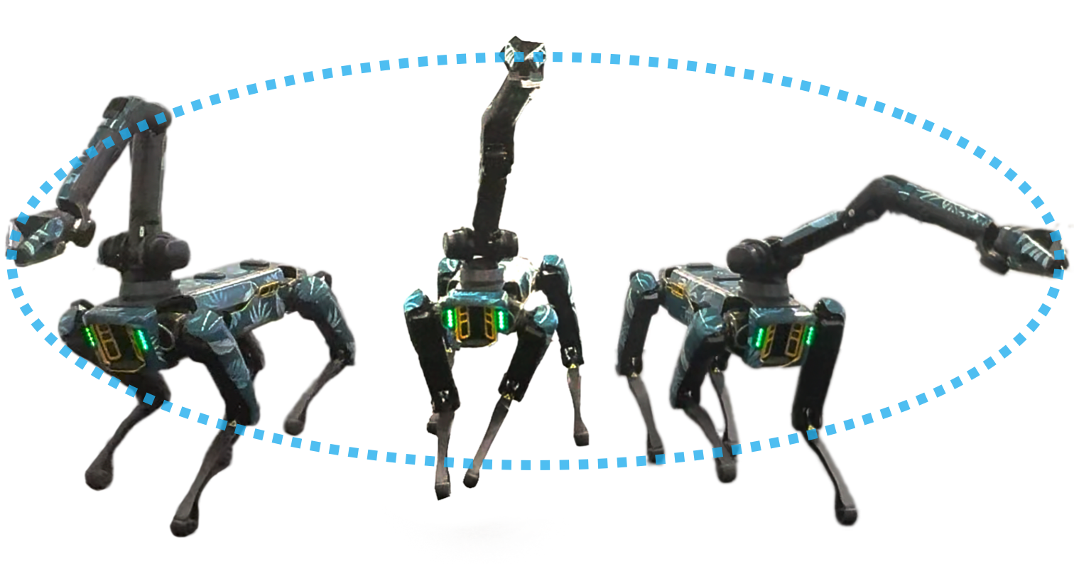
Figure 1: Boston Dynamics Spot with an attached arm tracking an ellipsoidal reference trajectory with its end-effector in our experiments.

II Related Work

II-A Legged Loco-Manipulation

Combining legged locomotion and manipulation to achieve platforms capable of dynamic mobile manipulation is an increasingly relevant problem that has been the focus of a considerable amount of research [24, 25, 22, 18, 20, 21, 26, 27, 28, 19, 14, 12, 13, 11, 29]. We can generally make a distinction between platforms that use a robot’s body [25, 22] or legs [18, 20, 21] for manipulation, those that apply a hybrid approach such as attaching a gripper to a leg [26, 27] or a net to the base [28], and those that use a dedicated arm [19, 14, 12, 13, 11, 29]. Especially this last category allows for combining the impressive advances in legged locomotion with the benefits of a capable manipulator, enabling advanced tasks such as grasping stationary items [14, 12, 13], opening doors [11] or wiping a whiteboard [14].

II-B Control for Loco-Manipulation

Due to the complexity of such a combined platform, loco-manipulation control is inherently a challenging, high-dimensional, and non-smooth control problem [19]. In [12], Zimmermann et al. create a platform similar to the one used in this project by attaching a Kinova arm to Boston Dynamics’ Spot quadruped, allowing it to perform advanced tasks in loco-manipulation such as statically and dynamically fetching stationary items. While [12] uses trajectory optimization to generate control policies in a feed-forward manner, we aim to pursue a closed-loop approach to allow for more robust and adaptive control.

To this end, RL has emerged as a powerful approach that enables robust legged locomotion in general [7, 30, 31, 32, 33, 34, 9, 8, 35, 36] and shows impressive performance in the complex setting of loco-manipulation [18, 19, 14, 20, 21, 22]. While these prior works mainly focus on using a model-free RL approach, recently model-based RL has shown potential for more sample-efficient robot learning across distinct locomotion and manipulation tasks. In [37], Wu et al. apply the Dreamer algorithm [38] for real-world robot learning and demonstrate how using a learned world model allows for more efficient policy learning in both quadruped locomotion and robotic arm manipulation. Motivated by this success, we leverage recent advances in the fields of model-based RL and dynamics learning, primarily Sim-FSVGD [17], to achieve improved sample-efficiency, good sim-to-real transfer performance and better generalization to new tasks, even when access to an accurate simulation environment is not freely available.

II-C Modeling Robot Dynamics

Although state-of-the-art quadrupeds like the Boston Dynamics Spot are very capable platforms, their usage in a research setting yields certain challenges. As a commercial product, knowledge of their built-in controller remains proprietary, and low-level control access is often restricted. However, an accurate system model is necessary to pursue a model-based or learning-based control method. To this end, [12] uses a simple parametrized dynamics model and parameter identification to simulate the platform’s behavior. Yet, accurately modeling the dynamics of a complex system like a quadruped with an attached arm is a challenging, dynamic, and high-DoF problem [14, 23]. In the simplistic approach of [12], the robot fails to achieve the desired task in certain cases due to the model’s inability to fully capture Spot’s complex internal behavior. Especially the wrench and disturbances introduced by the arm can be hard to model accurately.

These challenges lead us to opt for a more sophisticated modeling approach using both a hand-crafted kinematic model and BNNs to better capture the complex dynamics of the system. In [17], Rothfuss et al. introduce Sim-FSVGD, a BNN-based method to learn robot dynamics from data, which they test on hardware using a dynamic RC car. By incorporating low-fidelity physical priors, such as a kinematic simulator, during learning, they achieve improved sample-efficiency and sim-to-real transfer performance. Further, Bayesian Neural Networks do not tend to exhibit the same overfitting behavior as their non-bayesian counterparts [17]. These advancements allow us to develop an accurate model of our complex system by efficiently learning a BNN using prior knowledge from our kinematic model and to derive control policies capable of performing dynamic loco-manipulation tasks, even in low-data regimes.

III Preliminaries

III-A Model-Based Reinforcement Learning

In an RL setting, our problem of learning control policies for loco-manipulation can be formulated as a Markov Decision Process (MDP) defined by the tuple $(\mathcal{S},\mathcal{A},f,r,\gamma,\mathbf{s}_{0})$, where $\mathcal{S}$ is the state space, $\mathcal{A}$ the action space, $f:\mathcal{S}\times\mathcal{A}\rightarrow\mathcal{S}$ is the transition model or dynamics of the system, $r:\mathcal{S}\times\mathcal{A}\rightarrow\mathbb{R}$ the reward function, $\gamma\in(0,1)$ the discount factor, and $\mathbf{s}_{0}$ the initial state distribution. The goal of an RL approach is to then find an optimal policy $\pi^{*}$ that maximizes an agent’s performance in this setting. We can define the performance of a policy $\pi$ over a fixed horizon $H$ subject to the dynamics $\mathbf{s}_{t+1}\sim f(\mathbf{s}_{t},\mathbf{u}_{t})$ as the expected sum of discounted rewards over the horizon [39]:

$$J(\pi,f)=\mathbb{E}_{u_{t}\sim\pi}\left[\sum_{t=0}^{H}\gamma^{t}r(\mathbf{s}_{t},\mathbf{u}_{t})\mid\mathbf{s}_{0}\right].$$ (1)

Our desired optimal policy $\pi^{*}$ is then the result of the optimization problem

$$\pi^{*}=\arg\max_{\pi}J(\pi,f).$$ (2)

In practice, however, we often lack a model of the system dynamics $f$. Consequently, in model-based RL we aim first to learn an approximate model $\hat{f}$ of the dynamics from data collected by interacting with the real system. We then leverage this learned model to derive control policies that maximize our objective using an appropriate RL scheme.

III-B Learning Robot Dynamics

III-B1 Learning with NNs

In a robotics context, we want to use model-based RL to derive control policies that allow us to perform dynamic tasks with our platform, such as loco-manipulation. Learning an accurate dynamics model of our robot is thus necessary. For this purpose, we consider a time-discretized dynamical system described as

$$\mathbf{s}_{t+1}=f(\mathbf{s}_{t},\mathbf{u}_{t}),$$ (3)

where $\mathbf{s}_{t}\in\mathbb{R}^{n_{s}}$ is the state of the system at time $t$, $\mathbf{u}_{t}\in\mathbb{R}^{n_{u}}$ is the control input, and $f(\mathbf{s}_{t},\mathbf{u}_{t})$ is the unknown dynamics of the system. We now aim to learn a model $\hat{f}(\mathbf{s}_{t},\mathbf{u}_{t})$ that approximates the true dynamics of the system from a dataset of state-action-state transitions $(\mathbf{s}_{t},\mathbf{u}_{t},\mathbf{s}_{t+1})$. To this end, we can state our problem as learning an unknown dynamics function $\hat{f}:\mathcal{X}\rightarrow\mathcal{Y}$ from a dataset $\mathcal{D}=(\mathbf{X}^{\mathcal{D}},\mathbf{y}^{\mathcal{D}})$ of size $N$, where our training inputs consist of the state-action pairs $\mathbf{X}^{\mathcal{D}}=\{\mathbf{x}_{j}\}_{j=1}^{N}$ and the target outputs $\mathbf{y}^{\mathcal{D}}=\{\mathbf{y}_{j}\}_{j=1}^{N}$ are the measured noisy observations of our dynamics, i.e. $\mathbf{y}_{j}=f(\mathbf{x}_{j})+\epsilon_{j}$. We assume the noise $\epsilon$ to be i.i.d. and Gaussian with variance $\sigma^{2}$. Using a Neural Network (NN) to model $\hat{f}$, we can then formulate our learning problem as fitting a NN model $h_{\theta}:\mathcal{X}\rightarrow\mathcal{Y}$ with network weights $\theta$ from $\mathcal{D}$. We can use $h_{\theta}$ to define the conditional predictive distribution of our observations as

$$p(\mathbf{y}|\mathbf{x},\theta)=\mathcal{N}(\mathbf{y}|h_{\theta}(\mathbf{x}),\sigma^{2}).$$ (4)

III-B2 Learning with BNNs

This can be extended to learning a BNN by considering not only a single set of weights but a distribution over $\theta$. BNNs then infer a posterior distribution over the weights $p(\theta|\mathbf{X}^{\mathcal{D}},\mathbf{y}^{\mathcal{D}})\propto p(\mathbf{y}^{\mathcal{D}}|\mathbf{X}^{\mathcal{D}},\theta)p(\theta)$ given the data-likelihood $p(\mathbf{y}^{\mathcal{D}}|\mathbf{X}^{\mathcal{D}},\theta)$ and a known prior distribution $p(\theta)$. Under the assumption that, given $\theta$, each data point is conditionally independent, the likelihood can be factorized as $p(\mathbf{y}^{\mathcal{D}}|\mathbf{X}^{\mathcal{D}},\theta)=\prod_{j=1}^{N}p(\mathbf{y}_{j}|\mathbf{x}_{j},\theta)$. Finally, the predictive distribution for a new input $\mathbf{x}^{*}$ can be defined as

$$p(\mathbf{y}^{*}|\mathbf{x}^{*},\mathbf{X}^{\mathcal{D}},\mathbf{y}^{\mathcal{D}}) =\int p(\mathbf{y}^{*}|\mathbf{x}^{*},\theta)p(\theta|\mathbf{X}^{\mathcal{D}},\mathbf{y}^{\mathcal{D}})d\theta$$ (5)

$$=\mathbb{E}_{\theta}[p(\mathbf{y}^{*}|\mathbf{x}^{*},\theta)|\mathbf{X}^{\mathcal{D}},\mathbf{y}^{\mathcal{D}}]$$ (6)

by marginalizing over the weights $\theta$ [17].

III-C Function Space Inference and Functional Priors

III-C1 FSVGD

Performing posterior inference with BNNs, however, is challenging. Both the high-dimensionality of the weight space, as well as the over-parametrization of the mapping between $\theta$ and a likelihood function $p(\mathbf{y}^{\mathcal{D}}|\mathbf{X}^{\mathcal{D}},\theta)$ render inference difficult [17, 40]. The functional Stein Variational Gradient Descent (FSVGD) method [40] addresses these issues by performing BNN inference in the space of regression functions $h:\mathcal{X}\rightarrow\mathcal{Y}$, rather than in the weight space of $\theta$. In function space, the posterior is formulated as

$$p(h|\mathbf{X}^{\mathcal{D}},\mathbf{y}^{\mathcal{D}})\propto p(\mathbf{y}^{\mathcal{D}}|\mathbf{X}^{\mathcal{D}},h)p(h),$$ (7)

where $p(h)$ is a stochastic prior distribution over $h:\mathcal{X}\rightarrow\mathcal{Y}$ with index space $\mathcal{X}$ and value space $\mathcal{Y}$ [17, 41]. This allows for the functional inference to be restated in a tractable form by using finite measurement sets $\mathbf{X}:=[\mathbf{x}_{1},...,\mathbf{x}_{k}]\in\mathcal{X}^{k},k\in\mathbb{N}$ that allow for characterizing a stochastic process by marginals of function values $\rho(\mathbf{h}^{\mathbf{X}}):=\rho(h(\mathbf{x}_{1}),...,h(\mathbf{x}_{k}))$ and subsequently stating the functional posterior as

$$p(\mathbf{h}^{\mathbf{X}}|\mathbf{X},\mathbf{X}^{\mathcal{D}},\mathbf{y}^{\mathcal{D}})\propto p(\mathbf{y}^{\mathcal{D}}|\mathbf{X}^{\mathcal{D}},\mathbf{h}^{\mathbf{X}})p(\mathbf{h}^{\mathbf{X}}),$$ (8)

for the measurement sets $\mathbf{X}$ [17, 42]. FSVGD approximates this posterior by maintaining $L$ parameter particles ${\theta_{1},...,\theta_{L}}$ and iteratively re-sampling $\mathbf{X}$ as a random subset of $\mathcal{X}$ with $\mathbf{X}\sim\mu$ where $\mu$ is an arbitrary distribution supported on $\mathcal{X}$. FSVGD then updates the particles using

$$\theta_{l}=\theta_{l}-\gamma J_{l}u_{l},$$ (9)

where $J_{l}$ is the NN Jacobian and $u_{l}$ is the SVGD update [43] in function space [17]

$$J_{l} =(\nabla_{\theta_{l}}\mathbf{h}_{\theta_{l}}^{\mathbf{X}})^{\top},$$ (10)

$$u_{l} =\frac{1}{L}\sum_{i=1}^{L}\mathbf{K}_{li}\nabla_{\mathbf{h}_{\theta_{i}}^{\mathbf{x}}}\ln p(\mathbf{h}_{\theta_{l}}^{\mathbf{x}}|\mathbf{X},\mathbf{X}^{D},\mathbf{y}^{D})+\nabla_{\mathbf{h}_{\theta_{l}}^{\mathbf{x}}}\mathbf{K}_{li}.$$ (11)

Here $\mathbf{K}=[k(\mathbf{h}_{\theta_{l}}^{\mathbf{x}},\mathbf{h}_{\theta_{i}}^{\mathbf{x}})]_{li}$ is the gram matrix, based on a kernel function $k$, between the measurement points and the function values [17, 40].

III-C2 Sim-FSVGD

The Sim-FSVGD method [17] extends FSVGD by using an informed functional prior $p(h)$ for a function $h:\mathcal{X}\rightarrow\mathcal{Y}$ that incorporates both a domain-model process and a sim-to-real prior. Sim-FSVGD factorizes the prior over the output dimensions as $p(h)=\prod_{i=1}^{n_{s}}p(h_{i})$, treating each $h_{i}:\mathbf{X}\rightarrow\mathbb{R}$ as an independent function.

The domain-model process allows for the integration of domain-specific knowledge of the system, e.g. from first principles, by using a simulation model $g(\mathbf{x},\phi)$ where $\phi$ are the model parameters. As the exact model parameters are unknown, we can randomly sample them from a plausible range as $\phi\sim p(\phi)$ and create distinct simulation models per parameter set, implicitly creating a stochastic process of functions.

The sim-to-real prior addresses the gap between a simulation model and the actual system dynamics $f(\mathbf{x})$ by adding a sim-to-real gap process in form of a Gaussian Process (GP) $p(\tilde{h}_{i})$ per output dimension $i=1,...,n_{s}$. Sim-FSVGD uses a zero-mean GP with isotropic kernel $k(\mathbf{x},\mathbf{x}^{\prime})=\nu^{2}\rho(||\mathbf{x}-\mathbf{x}^{\prime}||/l)$, where the lengthscale $l$ and the variance $\nu^{2}$ are hyperparameters that allow us to represent our assumptions about the sim-to-real gap.

The combined stochastic process prior $p(h)$ is then defined implicitly via the marginal distributions implied by independently sampling conditional random vectors from each process and adding them, i.e.

$$\mathbf{h}_{i}^{\mathbf{x}}=\left[g_{i}(\mathbf{x}_{1},\phi),\dots,g_{i}(\mathbf{x}_{k},\phi)\right]^{\top}+\tilde{\mathbf{h}}_{i}^{\mathbf{x}},$$ (12)

where $\phi\sim p(\phi)$ and $\tilde{\mathbf{h}}^{\mathbf{X}}_{i}\sim\mathcal{N}(\tilde{\mathbf{h}}^{\mathbf{X}}_{i}|0,\mathbf{K})$ [17]. Lastly, Sim-FSVGD relies on the same update rule as in eq. 9 to update the particles $\theta_{l}$. The stochastic process prior score $\nabla_{\mathbf{h}^{\mathbf{X}}}\ln p(\mathbf{h}^{\mathbf{X}})=\sum_{i}^{n_{s}}\nabla_{\mathbf{h}^{\mathbf{X}}_{i}}\ln p(\mathbf{h}^{\mathbf{X}}_{i})$ is approximated using a Gaussian approximation of the prior process, i.e. $p(\mathbf{h}_{i}^{\mathbf{X}})\sim\mathcal{N}(\mu_{i}^{\mathbf{X}},\Sigma_{i}^{\mathbf{X}})$. The approximation is constructed by sampling the measurement set $\mathbf{X}$ from a distribution $\mu$ supported on $\mathcal{X}$, sampling $m=1,...,P$ vectors of function values $\mathbf{h}_{i,m}^{\mathbf{X}}\sim p(\mathbf{h}_{i}^{\mathbf{X}})$ and subsequently computing their mean $\mu_{i}^{\mathbf{X}}$ and covariance $\Sigma_{i}^{\mathbf{X}}$.

IV Learning Control Polices for Loco-Manipulation

Our work focuses on efficiently learning an accurate dynamics model of our robot from data to subsequently derive control policies for loco-manipulation tasks via model-based RL. To this end, we first develop a hand-crafted kinematic model $\hat{f}_{kin}$ of our quadruped-with-arm platform. We then use $\hat{f}_{kin}$ as a physical prior within the BNN-based method Sim-FSVGD to efficiently learn a model $\hat{f}$ from data that approximates our platform’s true dynamics $f$. Subsequently, we use our learned model $\hat{f}$ and develop a reward structure ${r}$ to learn a control policy $\pi$ for end-effector trajectory tracking using the Soft-Actor-Critic (SAC) method [44]. In this section, we first present our control approach, develop our kinematic model $\hat{f}_{kin}$ and show how we apply it within the Sim-FSVGD method to learn $\hat{f}$, and finally discuss our policy learning process.

IV-A Robot State and Control Input

Similarly to [12], let us denote our base state as the position, orientation and velocity of the robot’s base on a 2D plane in world frame $W$, i.e. $\mathbf{p}^{\text{base}}=[x^{\text{base}},y^{\text{base}},\theta^{\text{base}}]$ and $\mathbf{v}^{\text{base}}=[v_{x}^{\text{base}},v_{y}^{\text{base}},\omega^{\text{base}}]$. Here $\theta^{\text{base}}$ is the yaw angle of the robot’s base, and $\omega^{\text{base}}$ is the corresponding angular velocity. For the mounted end-effector, we represent the state using the position and velocity in 3D in world frame $W$, i.e. $\mathbf{p}^{\text{ee}}=[x^{\text{ee}},y^{\text{ee}},z^{\text{ee}}]$ and $\mathbf{v}^{\text{ee}}=[v_{x}^{\text{ee}},v_{y}^{\text{ee}},v_{z}^{\text{ee}}]$. We provide an overview of the respective frames in fig. 2. Stacking the individual components, we define the following state vector

$$\mathbf{s}=\begin{bmatrix}\mathbf{p}^{\text{base}}\\ \mathbf{v}^{\text{base}}\\ \mathbf{p}^{\text{ee}}\\ \mathbf{v}^{\text{ee}}\\ \end{bmatrix}\in\mathbb{R}^{12}.$$ (13)

We use velocity commands to control our robot. As the state representation suggests, for the base of the robot, we command the $v_{x}^{\text{base}}$, $v_{y}^{\text{base}}$ and $\omega^{\text{base}}$ velocities on a 2D plane. This results in the control input $\mathbf{u}^{\text{base}}=[u_{vx}^{\text{base}},u_{vy}^{\text{base}},u_{\omega}^{\text{base}}]$. We express the velocities in the body frame $B$ and apply them at the robot’s center of mass. For the end-effector, we command the $v_{x}^{\text{ee}}$, $v_{y}^{\text{ee}}$ and $v_{z}^{\text{ee}}$ velocities in 3D, i.e. $\mathbf{u}^{\text{ee}}=[u_{vx}^{\text{ee}},u_{vy}^{\text{ee}},u_{vz}^{\text{ee}}]$. Again, the velocities are expressed in the body frame $B$ and are applied at the center of the end-effector frame $H$, which sits at the center of the gripper. Our control input is then given as

$$\mathbf{u}=\begin{bmatrix}\mathbf{u}^{\text{base}}\\ \mathbf{u}^{\text{ee}}\end{bmatrix}\in\mathbb{R}^{6}.$$ (14)

In this work, we choose velocity control over joint control for both the base and the end-effector since, at the commencement of our project, low-level control access for the Boston Dynamics Spot remained restricted. Further, this lower-dimensional input allows us to efficiently collect real transition data on the robot via manual teleoperation, as it simplifies the mapping between a joystick controller and the control input.

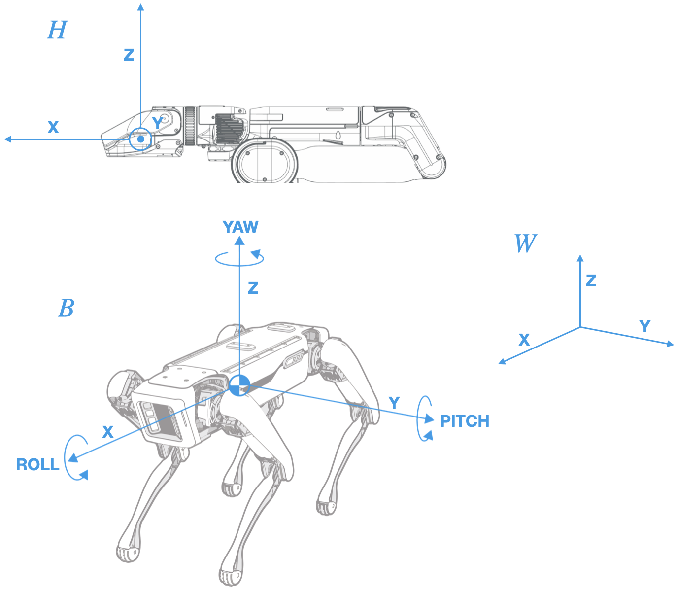
Figure 2: We use the Boston Dynamics Spot quadruped and its arm as our loco-manipulation platform. Here, we provide an overview of the robot and its arm adapted from [45], along with the end-effector frame $H$, the body frame $B$, and the world frame $W$.

IV-B Developing a Dynamics Model

Akin to our derivation in section III, we model the dynamics of our robot as the time discretized system $\mathbf{s}_{t+1}=\hat{f}(\mathbf{s}_{t},\mathbf{u}_{t})$, where $\mathbf{s}_{t}\in\mathbb{R}^{n_{s}}$ is the state of the system at time $t$, $\mathbf{u}_{t}\in\mathbb{R}^{n_{u}}$ is the control input, and $\hat{f}(\mathbf{s}_{t},\mathbf{u}_{t})$ is the approximated dynamics of the system. Following our state and input definitions in eq. 13 and eq. 14, our state dimensionality is $n_{s}=12$ and our control input dimensionality is $n_{u}=6$. We now develop our dynamics model in two steps. First, we create a hand-crafted kinematic model $\hat{f}_{kin}$ of our robot derived from first principles. In a second step, we then use this model as a physical prior within the BNN-based method Sim-FSVGD to efficiently learn a dynamics model $\hat{f}$ from real-world data.

IV-B1 Kinematic Model

We derive our kinematic model from first principles and use the Forward Euler Method with time step $\Delta t$ to propagate our state. To better capture the complex dynamics of our quadruped-with-arm platform, we enhance our equations with the parameters $\mathbf{\alpha}\in\mathbb{R}^{6\times 1}$, $\mathbf{\beta}\in\mathbb{R}^{12\times 1}$, and $\mathbf{\gamma}\in\mathbb{R}^{6\times 1}$. As our actions $\mathbf{u}_{t}$ are given in the body frame $B$ and our state $\mathbf{s}_{t}$ is in the world frame $W$, we first convert our inputs to $\mathbf{u}_{t}^{W}$ using the base’s current yaw angle $\theta^{\text{base}}_{t}$, i.e.

$$\mathbf{u}_{t}^{W} =\begin{bmatrix}\cos(\theta_{t}^{\text{base}})\cdot u_{vx,t}^{\text{base},B}-\sin(\theta_{t}^{\text{base}})\cdot u_{vy,t}^{\text{base},B}\\ \sin(\theta_{t}^{\text{base}})\cdot u_{vx,t}^{\text{base},B}+\cos(\theta_{t}^{\text{base}})\cdot u_{vy,t}^{\text{base},B}\\ u_{\omega,t}^{\text{base},B}\\ \cos(\theta_{t}^{\text{base}})\cdot u_{vx,t}^{\text{ee},B}-\sin(\theta_{t}^{\text{base}})\cdot u_{vy,t}^{\text{ee},B}\\ \sin(\theta_{t}^{\text{base}})\cdot u_{vx,t}^{\text{ee},B}+\cos(\theta_{t}^{\text{base}})\cdot u_{vy,t}^{\text{ee},B}\\ u_{vz,t}^{\text{ee},B}\end{bmatrix}.$$ (15)

We can then derive the update equations for the base velocity $\mathbf{v}^{\text{base}}$ and position $\mathbf{p}^{\text{base}}$ as

$$\mathbf{v}_{t+1}^{\text{base}} =\begin{bmatrix}\alpha_{1}v_{x,t}^{\text{base}}+(1-\alpha_{1})u_{vx,t}^{\text{base},W}+\beta_{1}\\ \alpha_{2}v_{y,t}^{\text{base}}+(1-\alpha_{2})u_{vy,t}^{\text{base},W}+\beta_{2}\\ \alpha_{3}\omega_{t}^{\text{base}}+(1-\alpha_{3})u_{\omega,t}^{\text{base},W}+\beta_{3}\end{bmatrix},$$ (16)

$$\mathbf{p}_{t+1}^{\text{base}} =\begin{bmatrix}x_{t}^{\text{base}}+\Delta t\,v_{x,t+1}^{\text{base}}\gamma_{1}+\beta_{4}\\ y_{t}^{\text{base}}+\Delta t\,v_{y,t+1}^{\text{base}}\gamma_{2}+\beta_{5}\\ \theta_{t}^{\text{base}}+\Delta t\,\omega_{t+1}^{\text{base}}\gamma_{3}+\beta_{6}\end{bmatrix}.$$ (17)

For the end-effector updates, we need to consider the base’s movements in addition to the end-effector velocity commands. Incorporating the horizontal linear velocities of the base $v_{x,t}^{\text{base}}$ and $v_{y,t}^{\text{base}}$ follows simply via addition. However, to consider the base’s angular velocity $\omega_{t}^{\text{base}}$ in the end-effector’s movement, we first need to calculate the induced velocity on the end-effector $\mathbf{v}^{\text{ind}}$ as

$$\mathbf{v}^{\text{ind}}=\begin{bmatrix}-\omega_{t+1}^{\text{base}}\cdot d\cdot\sin(\phi)\\ \omega_{t+1}^{\text{base}}\cdot d\cdot\cos(\phi)\\ 0\end{bmatrix},$$ (18)

where $d=\sqrt{\left(x_{t}^{\text{ee}}-x_{t}^{\text{base}}\right)^{2}+\left(y_{t}^{\text{ee}}-y_{t}^{\text{base}}\right)^{2}}$ is the distance between the base’s rotational axis and the end-effector, and $\phi=\mathrm{arctan2}\left(y_{t}^{\text{ee}}-y_{t}^{\text{base}},\,x_{t}^{\text{ee}}-x_{t}^{\text{base}}\right)$ is the angle of the induced velocity vector in the global frame $W$. We can then update the end-effector velocity $\mathbf{v}^{\text{ee}}$ and position $\mathbf{p}^{\text{ee}}$ as

$$\mathbf{v}_{t+1}^{\text{ee}} =\begin{bmatrix}\alpha_{4}\,v_{x,t}^{\text{ee}}+(1-\alpha_{4})\,u_{vx,t}^{\text{ee},W}+\beta_{7}\\ \alpha_{5}\,v_{y,t}^{\text{ee}}+(1-\alpha_{5})\,u_{vy,t}^{\text{ee},W}+\beta_{8}\\ \alpha_{6}\,v_{z,t}^{\text{ee}}+(1-\alpha_{6})\,u_{vz,t}^{\text{ee},W}+\beta_{9}\end{bmatrix}+\begin{bmatrix}v_{x,t+1}^{\text{base}}\\ v_{y,t+1}^{\text{base}}\\ 0\end{bmatrix}+\mathbf{v}^{\text{ind}},$$ (19)

$$\mathbf{p}_{t+1}^{\text{ee}} =\begin{bmatrix}x_{t}^{\text{ee}}+\Delta t\,v_{x,t+1}^{\text{ee}}\,\gamma_{4}+\beta_{10}\\ y_{t}^{\text{ee}}+\Delta t\,v_{y,t+1}^{\text{ee}}\,\gamma_{5}+\beta_{11}\\ z_{t}^{\text{ee}}+\Delta t\,v_{z,t+1}^{\text{ee}}\,\gamma_{6}+\beta_{12}\end{bmatrix}.$$ (20)

IV-B2 BNN Model

To learn a BNN model of our robot from data, we use the Sim-FSVGD method [17], as detailed in section III. Sim-FSVGD allows us to use our kinematic model $\hat{f}_{kin}$ to create the domain-model process, where our system parameters $\phi$ are thus the set of parameters used in our update equations, i.e. $\phi=[\mathbf{\alpha},\mathbf{\beta},\mathbf{\gamma}]\in\mathbb{R}^{24\times 1}$. Note that, as Sim-FSVGD randomly samples parameter sets as $\phi\sim p(\phi)$ to implicitly create a stochastic process of functions, we do not deterministically fit the parameters of our kinematic model from data. However, we use real-world data to estimate a plausible range for our parameters. We then use the same sim-to-real prior and implementation as in [17], which we summarize in section III, to learn our dynamics model $\hat{f}$ from real-world data.

IV-C Policy Learning

Having learned a model of our system, we can now turn to learning control policies for loco-manipulation tasks using RL. To this end, we employ the SAC algorithm [44] to obtain a control policy $\pi$. As we aim to perform tasks in loco-manipulation, our policy is conditioned on end-effector goal positions $\mathbf{g}^{\text{ee}}$ in world frame $W$, i.e. $\mathbf{g}^{\text{ee}}=[x_{g}^{W},y_{g}^{W},z_{g}^{W}]$. To achieve this, we uniformly sample an initial state $\mathbf{s}_{0}$ and end-effector goal position $\mathbf{g}^{\text{ee}}$ within a specified range at the beginning of each episode. We then append the goal position to the state vector $\mathbf{s}$, creating a goal conditioned state vector for policy learning $\mathbf{s}_{\text{cond}}=[\mathbf{s},\mathbf{g}^{\text{ee}}]\in\mathbb{R}^{15\times 1}$, while our action space remains our control input $\mathbf{u}\in\mathbb{R}^{6\times 1}$.

To guide our policy learning, we design a reward structure $r(\mathbf{s}_{\text{cond}},\mathbf{u})$ that encourages the end-effector to move towards the goal position while keeping the end-effector within a physically valid range from the base and penalizing large control inputs. Our reward structure is thus threefold consisting of (i) a state-goal distance reward $r_{\text{state}}$, (ii) an end-effector to base distance reward $r_{\text{ee-base}}$ and (iii) a regularizing action reward $r_{\text{action}}$.

(i) $r_{\text{state}}$

We use this component to drive the end-effector towards a goal position. To this end, we employ a reward function that assigns a full reward when the distance $d_{\text{ee-goal}}=\lVert\mathbf{p}^{\text{ee}}-\mathbf{g}^{\text{ee}}\rVert$ between the end-effector position $\mathbf{p}^{\text{ee}}$ and the goal position $\mathbf{g}^{\text{ee}}$ lies within a specified bound $(0,b)$. Outside these bounds, we smoothly decrease the reward using a long-tailed sigmoid function $\sigma_{m,a}(x)=\left(\left(xm^{-1}\sqrt{a^{-1}-1}\right)^{2}+1\right)^{-1}$ [46], with a defined value $a$ at margin $m$, creating a smooth reward with infinite-support and range $[0,1]$.

$$r_{\text{state}}(\mathbf{s}_{\text{cond}})=\begin{cases}1,&d_{\text{ee-goal}}\leq b,\\[6.0pt] \sigma_{m,a}\!\biggl{(}d_{\text{ee-goal}}-b\biggr{)}&d_{\text{ee-goal}}>b\end{cases}$$ (21)

(ii) $r_{\text{ee-base}}$

The second component encourages the distance $d_{\text{ee-base}}=\lVert\mathbf{p}^{\text{ee}}-\mathbf{p}^{\text{base}}\rVert$ between the end-effector position $\mathbf{p}^{\text{ee}}$ and the base position $\mathbf{p}^{\text{base}}$ to stay within a physically valid range given by the arm’s length $l_{\text{arm}}$. To achieve this, we use the same approach as in (i) with the bounds $(0,l_{\text{arm}})$.

$$r_{\text{ee-base}}(\mathbf{s}_{\text{cond}})=\begin{cases}1,&d_{\text{ee-base}}\leq l_{\text{arm}},\\[6.0pt] \sigma_{m,a}\!\biggl{(}d_{\text{ee-base}}-l_{\text{arm}}\biggr{)}&d_{\text{ee-base}}>l_{\text{arm}}\end{cases}$$ (22)

(iii) $r_{\text{action}}$

Lastly, we include an action cost term that penalizes inefficient policies. However, instead of weighting each control input equally, we encourage the use of end-effector movements over body movements by assigning a higher weight $\lambda_{\text{base}}$ to the base actions than the end-effector actions weight $\lambda_{\text{ee}}$.

$$r_{\text{action}}(\mathbf{u})=-\left(\lambda_{\text{base}}\lVert\mathbf{u}^{\text{base}}\rVert^{2}+\lambda_{\text{ee}}\lVert\mathbf{u}^{\text{ee}}\rVert^{2}\right)$$ (23)

We calculate our final reward as a weighted sum of the three components, i.e. $r(\mathbf{s}_{\text{cond}},\mathbf{u})=w_{1}r_{\text{state}}(\mathbf{s}_{\text{cond}})+w_{2}r_{\text{ee-base}}(\mathbf{s}_{\text{cond}})+w_{3}r_{\text{action}}(\mathbf{u})$, where $w_{1}$, $w_{2}$, and $w_{3}$ are the weight for each component which we tune heuristically.

V Experiments and Results

In this section, we present our experiments and results, which aim to evaluate the effectiveness of our model-based RL approach at learning dynamic loco-manipulation control policies for a complex quadruped-with-arm platform. To this end, we compare the performance of the dynamics model learned using our kinematic model and the Sim-FSVGD approach, which we simply label Sim-FSVGD, to two baseline models, Sim-MODEL and FSVGD, across different sample sizes. We evaluate both the sim-to-real transfer performance of the models as well as the real-world loco-manipulation performance of the control policies derived from them.

In the following, we first briefly detail our baseline models. Subsequently, we introduce our experiment platform, the Boston Dynamics Spot quadruped, as well as our data collection and data processing steps. Finally, we introduce our three experiments, Sim-to-Real Transfer and our hardware experiments Ellipse Tracking and Helix Tracking, and present the results of our evaluation.

V-A Baseline Models

We consider two baseline models, Sim-MODEL and FSVGD [40]. Sim-MODEL is our hand-crafted kinematic model with the parameters $\mathbf{\alpha}$, $\mathbf{\beta}$, and $\mathbf{\gamma}$ fitted from real-world data using the gradient-based optimizer Adam [47]. Notably, we use an unfitted version of the same kinematic model to create a low-fidelity physical prior in the Sim-FSVGD approach. FSVGD is a BNN-based method widely applied in deep learning, which we describe closer in section III. Contrary to Sim-FSVGD, FSVGD does not use an informed prior.

V-B Experiment Setup

V-B1 Boston Dynamics Spot Quadruped

For our experiments, we use the Boston Dynamics Spot, a state-of-the-art quadruped robot equipped with an arm for manipulation. The robot allows for our control input to be passed and provides measurements of its current state over WiFi via a PC and a high-level Python SDK interface. Spot uses an unknown state-estimator, which computes the robot’s state from a combination of onboard motion sensors and cameras, as well as an unknown onboard controller that processes our control inputs. We provide an overview of Spot and its arm, along with the respective coordinate frames, in fig. 2.

V-B2 Data Collection

We collect our training data by directly interacting with our robot and manually controlling its base $\mathbf{v}^{\text{base}}$ velocities using an Xbox controller and its end-effector $\mathbf{v}^{\text{ee}}$ velocities using a 3D Space Mouse. In this fashion, we collect transitions consisting of the current state $\mathbf{s}_{t}$, the commanded action $\mathbf{u}_{t}$, and the next state $\mathbf{s}_{t+1}$. We collect transitions and command the robot at a frequency of $15\text{\,}\mathrm{Hz}$.

V-B3 Data Processing

Instead of using our dynamics model to predict the next system state directly, we opt to predict the change in the state. Therefore, we have to adapt our collected training data set accordingly by creating a new set where our input still consists of the state action pair $\mathbf{x}_{t}=[\mathbf{s}_{t},\mathbf{u}_{t}]$ but our new target output is simply the difference between the next state and the current state, i.e. $\mathbf{y}_{t}=[\mathbf{s}_{t+1}-\mathbf{s}_{t}]$. Additionally, we encode the base’s yaw angle $\theta^{base}$ as $(\sin(\theta^{base}),\cos(\theta^{base}))$ to avoid the discontinuity of the Euler angle representation at $-\pi$ and $\pi$, providing a representation more suitable for NNs [48]. Further, our control setup has a delay (ca. two timesteps, i.e.  $133\text{\,}\mathrm{ms}$) between the command and execution of an action. To compensate for this, we append the previous two actions $[\mathbf{u}_{t-2},\mathbf{u}_{t-1}]$ to the state $\mathbf{s}_{t}$, creating an augmented state $\mathbf{s}_{t}^{stacked}$. Our model input is thus $\mathbf{x}_{t}=[\mathbf{s}_{t}^{stacked},\mathbf{u}_{t}]=[\mathbf{s}_{t},\mathbf{u}_{t-2},\mathbf{u}_{t-1},\mathbf{u}_{t}]\in\mathbb{R}^{31\times 1}$ while our target output is $\mathbf{y}_{t}=[\mathbf{s}_{t+1}-\mathbf{s}_{t}]\in\mathbb{R}^{13\times 1}$. We then create a training set for supervised learning by sampling i.i.d. from the collected transitions.

V-C Sim-to-Real Transfer

Spot’s complex internal controller behavior, along with the wrench and disturbances produced by the arm, introduce behavior that is challenging to model accurately and is not captured in our kinematic model. To evaluate how well our approach performs at sim-to-real transfer for our quadruped-with-arm platform, we conduct a similar experiment to [17]. We train the Sim-FSVGD and FSVGD models on a dataset sampled i.i.d. from transitions collected on the real robot. We use the same dataset to fit the parameters of our Sim-MODEL. We evaluate the sim-to-real performance using the negative log-likelihood (NLL) of our model on a test dataset. We evaluate the sim-to-real transfer performance of the Sim-FSVGD model compared to our baselines and across different sample sizes used for learning. We use the sample sizes $N=\{500,1000,2000,3000,4000,5000\}$. We repeat our experiment with three different random seeds and average the NLL values across the seeds.

We present our results in fig. 3. From the results, we conclude that Sim-FSVGD outperforms FSVGD across all sample sizes. Especially in low data regimes, our simulation prior helps Sim-FSVGD achieve NLL scores significantly lower than FSVGD, while their NLL values converge as we add more samples. At $N=1000$ Sim-FSVGD performs similarly to our kinematic Sim-MODEL, surpassing it and achieving better scores for $N\geq 2000$. While the BNN-based models improve with the growing sample sizes, our kinematic Sim-MODEL achieves rather consistent NLL across all sample sizes, which is expected as we are fitting $24$ parameters using an abundant amount of data.

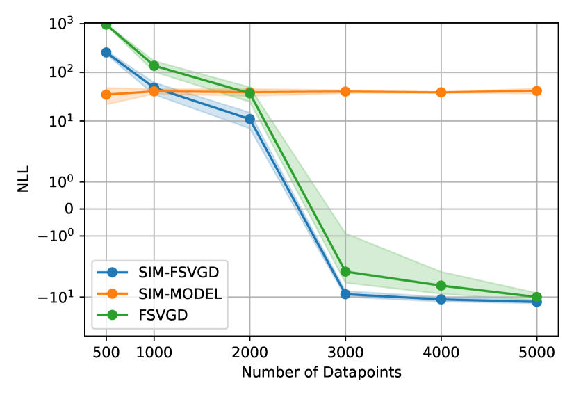
Figure 3: We compare the sim-to-real transfer performance for the dynamics models across different sample sizes. The NLL is evaluated on a test dataset collected on the real robot. The average NLL value across three seeds is displayed along with the standard error. Sim-FSVGD outperforms FSVGD across all sample sizes, especially in low data regimes, and performs better than our kinematic Sim-MODEL from $N\geq 2000$ onwards.

V-D Shape Tracking

We leverage our learned dynamics model to develop control policies for loco-manipulation via model-based RL as described in section IV. In this experiment, we evaluate the effectiveness of our approach on hardware by using the learned policy to dynamically track two shapes with the robot’s end-effector: (i) an ellipse and (ii) a helix. To create the reference trajectories, we sample points along the shape and pass them as end-effector goals $\mathbf{g}_{\text{ee}}$ to the goal-conditioned policy, switching to the next goal at every second timestep. To demonstrate our setup, we show Spot in our experiment space tracking an ellipsoidal goal trajectory in fig. 6.

Again, we compare the performance of policies learned using the Sim-FSVGD dynamics model to our baseline models across different sample sizes used for training. We use the same sample sizes as in the sim-to-real transfer experiment, i.e. $N=\{500,1000,2000,3000,4000,5000\}$, and repeat the experiment with three different random seeds. We evaluate the performance of our approach by analysing the mean error the learned policies achieve across the reference trajectory, i.e. $\frac{1}{T}\sum_{t=1}^{T}||\mathbf{p}_{t}^{\text{ee}}-\mathbf{g}_{t}^{\text{ee}}||_{2}$, where $\mathbf{g}_{t}^{\text{ee}}$ is the end-effector goal position at time $t$.

(i) Ellipse

Our quantitative results for the ellipse shape are presented in fig. 4, and the realized trajectories are plotted in fig. 4. From the figures, we observe that the policies learned using the Sim-FSVGD model clearly outperform those using FSVGD and our kinematic Sim-MODEL across all sample sizes. From fig. 4 we can see that, especially at smaller sample sizes ($N<3000$), our simulation prior helps Sim-FSVGD achieve significantly lower errors than both FSVGD (147.38% higher error at $N=2000$) and Sim-MODEL (152.69% higher error at $N=2000$). The performance of the policies learned using the FSVGD model tends to improve with the growing sample sizes as the model performance improves. However, even at $N=5000$ the error they achieve is still 12.17% higher than the error achieved by the policies learned using the Sim-FSVGD model at $N=1000$.

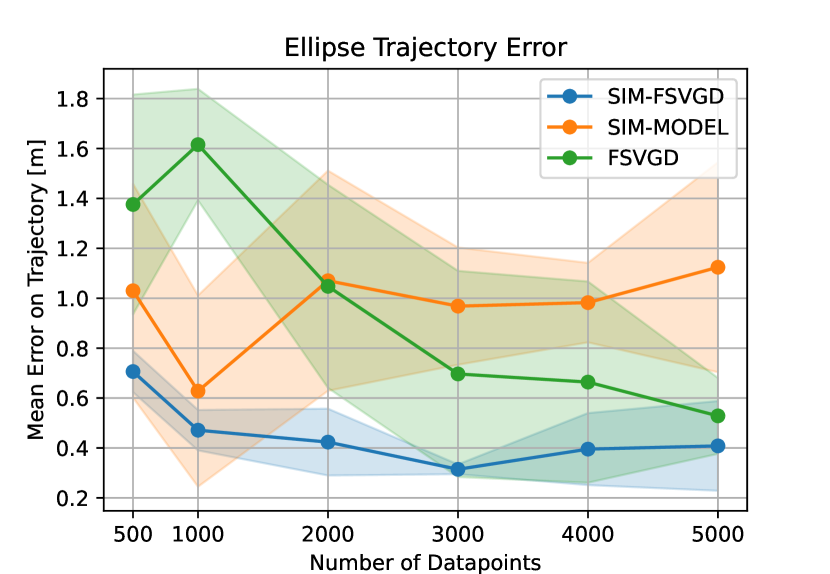
Figure 4: We plot the mean error our policies achieve on the ellipsoidal goal trajectory across different sample sizes used for learning. The average error across three seeds is displayed along with the standard deviation. We can observe that the policies learned using the Sim-FSVGD model outperform those learned using FSVGD and our kinematic Sim-MODEL across all sample sizes and especially at smaller sample sizes ($N<3000$).

(ii) Helix

We can observe similar results when evaluating the performance on the more challenging helix shape, which, due to its 3D nature, requires the end-effector to track a trajectory in all three dimensions. Notably, when observing the quantitative results in fig. 5, we see that again the policies learned using the Sim-FSVGD model significantly outperform those using FSVGD and our kinematic Sim-MODEL across all sample sizes. Again, even at $N=5000$, the error achieved by the policies learned using the FSVGD model is still 7.46% higher than the error achieved by the policies learned using the Sim-FSVGD model at $N=1000$.

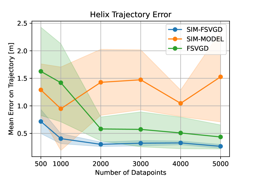
Figure 5: We plot the mean error our policies achieve on the helix goal trajectory across the different sample sizes used for learning. The average error across three seeds is displayed along with the standard deviation. Again, the policies learned using the Sim-FSVGD model clearly outperform those learned using FSVGD and our kinematic Sim-MODEL across all sample sizes.

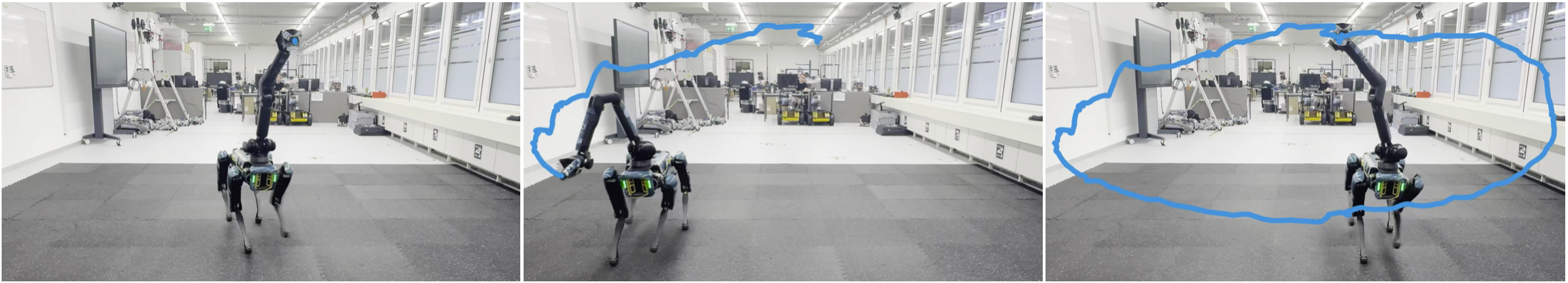
Figure 6: Spot in our experiment space tracking an ellipsoidal goal trajectory during our shape tracking experiments. In blue, we show the realized trajectory of the end-effector.

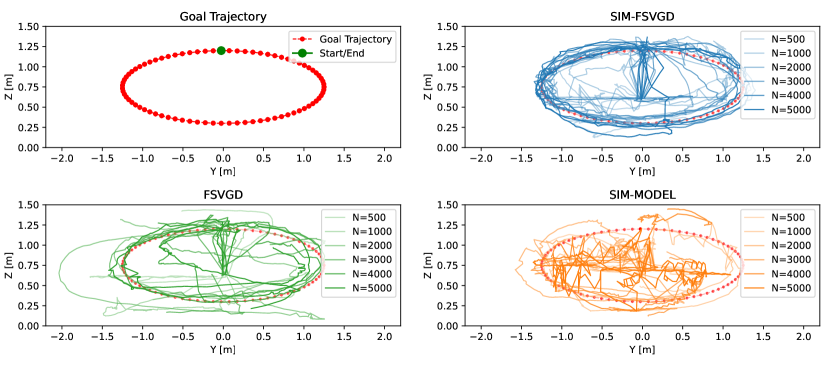
Figure 7: The ellipsoidal goal trajectory is shown on the top left plot. We plot the realized trajectories of the different policies on top of the goal trajectory for the dynamics models across all sample sizes and seeds. If a trajectory was on course for collision during our experiments, we stopped the trajectory early and plot only a truncated version. The initial position of the end-effector and the first goal are not equivalent, which can be seen in the lines connecting the center of the ellipse and the first goal. Qualitatively, we can observe that the policies learned using the Sim-FSVGD model follow the reference trajectory more closely than those learned using FSVGD and our kinematic Sim-MODEL.

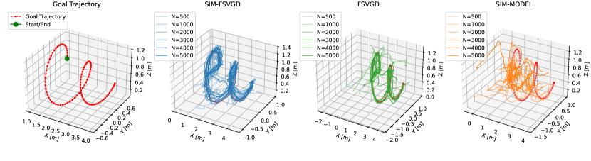
Figure 8: The 3D helix goal trajectory is shown on the top left plot. We plot the realized trajectories of the different policies on top of the goal trajectory for the dynamics models across all sample sizes and seeds. Again, if a trajectory was on course for collision during our experiments, we stopped the trajectory early and plot only a truncated version. The initial position of the end-effector and the first goal are not equivalent, which can be seen in the lines connecting the center of the helix and the first goal. For the helix, our qualitative observations are even more significant than for the ellipse, with the policies learned using the Sim-FSVGD model following the reference trajectory more closely than those learned using the baseline models.

The realized trajectories for both shapes, shown in fig. 7 and fig. 8, underline our quantitative results. Generally, we can observe that the policies learned using the Sim-FSVGD model follow the reference trajectory more closely than those learned using the baseline models. These findings on hardware demonstrate the effectiveness of our approach at learning loco-manipulation control policies for a complex quadruped-with-arm platform. We show that using our hand-crafted kinematic prior within the Sim-FSVGD methods allows for learning a model and control policies that achieve improved dynamic tracking performance over our baselines even in low-data regimes.

VI Conclusion

In this work, we address the problem of learning control policies for loco-manipulation tasks on a quadruped platform with an attached manipulator. We use a hand-crafted kinematic model and leverage advances in dynamics learning with BNNs, i.e. Sim-FSVGD [17], to efficiently learn a dynamics model of our system from limited data. In our experiments, we then leverage this learned dynamics model to derive loco-manipulation policies via RL, showing improved dynamic end-effector trajectory tracking accuracy even at reduced data requirements compared to baseline methods. Our results demonstrate the effectiveness of this approach on a complex commercial system with a proprietary, black-box nature such as the Boston Dynamics Spot quadruped with a manipulator.

Our approach shows certain shortcomings that could be addressed in future work. Although our tracked trajectories cover 3D space, they do not fully exploit the dynamic capabilities of the platform. Future work could investigate more complex trajectories that require fast, dynamic motion of the base, such as catching a ball. Further, our current state and action space does not include the end-effector’s orientation. Exploring how to incorporate these additional degrees of freedom into our model and control policies in future work could be beneficial for performing more complex loco-manipulation tasks.

-A Model and Policy Learning Hyperparameters

In this section, we provide the hyperparameters we used during our experiments. We list the hyperparameters used for learning the Sim-FSVGD dynamics model, as well as the two baseline models FSVGD and Sim-MODEL, in table I. In table II, we provide the SAC and reward hyperparameters used for loco-manipulation policy learning.

General BNN Hyperparameters
Particles	5
Batch size	64
Epochs	100
Max. training steps	200’000
Learning rate	1e-3
Weight decay	1e-3
Hidden layer sizes	64, 64, 64
Hidden activation function	LeakyReLU
Learn likelihood std	Yes
Likelihood exponent	1.0
Predict state difference	Yes
FSVGD Hyperparameters
Bandwidth SVGD	5.0
Lengthscale GP prior	0.2
Outputscale GP prior	1.0
Measurement points	16
Sim-FSVGD Hyperparameters
Bandwidth SVGD	5.0
Lengthscale simulation prior	1.0
Outputscale simulation prior	0.2
Measurement points	64
Function samples	256
Score estimator	GP
Sim-MODEL Hyperparameters
Optimizer	Adam [47]
Training steps	10’000
Learning rate	1e-3
Weight decay	1e-3

TABLE I: Hyperparameters for model learning used in our experiments.

SAC Hyperparameters
Environment steps	2’500’000
Episode length	120
Action repeat	1
Environment steps between updates	16
Environments	64
Evaluation environments	128
Learning rate $\alpha$	1e-4
Learning rate policy	1e-4
Learning rate q	1e-4
Weight decay $\alpha$	0.0
Weight decay policy	0.0
Weight decay q	0.0
Max. gradient norm	100
Discounting	0.99
Batch size	64
Evaluations	20
Reward scaling	1.0
$\tau$	0.005
Min. replay size	2048
Max. replay size	50’000
Gradient updates per step	1024
Policy hidden layer	64, 64
Policy activation function	Swish
Critic hidden layer	64, 64
Critic activation function	Swish
Reward Hyperparameters
$r_{\text{state}}$ bound $b$	0.15
$r_{\text{state}}$ margin $m$	1.5
$r_{\text{state}}$ value $a$ at margin	0.1
$r_{\text{ee-base}}$ bound $l_{\text{arm}}$	1.3
$r_{\text{ee-base}}$ margin $m$	1.3
$r_{\text{ee-base}}$ value $a$ at margin	0.1
$r_{\text{action}}$ base action weight $\lambda_{\text{base}}$	2.0
$r_{\text{action}}$ end-effector action weight $\lambda_{\text{ee}}$	0.5
$r_{\text{state}}$ weight $w_{1}$	1.5
$r_{\text{ee-base}}$ weight $w_{2}$	0.01
$r_{\text{action}}$ weight $w_{3}$	0.1

TABLE II: Hyperparameters for policy learning used in our experiments.

References

- Zhuang et al. [2023] Z. Zhuang, Z. Fu, J. Wang, C. Atkeson, S. Schwertfeger, C. Finn, and H. Zhao, “Robot Parkour Learning,” in Conference on Robot Learning (CoRL), 2023.
- Jenelten et al. [2024] F. Jenelten, J. He, F. Farshidian, and M. Hutter, “DTC: Deep Tracking Control,” Science Robotics, 2024.
- Yang et al. [2023] R. Yang, G. Yang, and X. Wang, “Neural volumetric memory for visual locomotion control,” 2023.
- Li et al. [2023a] C. Li, M. Vlastelica, S. Blaes, J. Frey, F. Grimminger, and G. Martius, “Learning agile skills via adversarial imitation of rough partial demonstrations,” in Proceedings of The 6th Conference on Robot Learning (CORL), 2023.
- Cheng et al. [2024] X. Cheng, K. Shi, A. Agarwal, and D. Pathak, “Extreme Parkour with Legged Robots,” in 2024 IEEE International Conference on Robotics and Automation (ICRA), 2024.
- Hoeller et al. [2024] D. Hoeller, N. Rudin, D. Sako, and M. Hutter, “ANYmal parkour: Learning agile navigation for quadrupedal robots,” Science Robotics, 2024.
- Choi et al. [2023] S. Choi, G. Ji, J. Park, H. Kim, J. Mun, J. H. Lee, and J. Hwangbo, “Learning quadrupedal locomotion on deformable terrain,” Science Robotics, 2023.
- Lee et al. [2020] J. Lee, J. Hwangbo, L. Wellhausen, V. Koltun, and M. Hutter, “Learning quadrupedal locomotion over challenging terrain,” Science Robotics, 2020.
- Kumar et al. [2021] A. Kumar, Z. Fu, D. Pathak, and J. Malik, “RMA: Rapid Motor Adaptation for Legged Robots,” in Robotics: Science and Systems XVII, 2021.
- Li et al. [2023b] C. Li, S. Blaes, P. Kolev, M. Vlastelica, J. Frey, and G. Martius, “Versatile skill control via self-supervised adversarial imitation of unlabeled mixed motions,” in 2023 IEEE international conference on robotics and automation (ICRA), 2023.
- Bellicoso et al. [2019] C. D. Bellicoso, K. Kramer, M. Stauble, D. Sako, F. Jenelten, M. Bjelonic, and M. Hutter, “ALMA - Articulated Locomotion and Manipulation for a Torque-Controllable Robot,” in 2019 International Conference on Robotics and Automation (ICRA), 2019.
- Zimmermann et al. [2021] S. Zimmermann, R. Poranne, and S. Coros, “Go Fetch! - Dynamic Grasps using Boston Dynamics Spot with External Robotic Arm,” in 2021 IEEE International Conference on Robotics and Automation (ICRA), 2021.
- Liu et al. [2024] M. Liu, Z. Chen, X. Cheng, Y. Ji, R.-Z. Qiu, R. Yang, and X. Wang, “Visual Whole-Body Control for Legged Loco-Manipulation,” arXiv, 2024.
- Fu et al. [2022] Z. Fu, X. Cheng, and D. Pathak, “Deep whole-body control: Learning a unified policy for manipulation and locomotion,” in Conference on Robot Learning (CoRL), 2022.
- Li et al. [2024] C. Li, E. Stanger-Jones, S. Heim, and S. Kim, “Fld: Fourier latent dynamics for structured motion representation and learning,” arXiv preprint arXiv:2402.13820, 2024.
- Moerland et al. [2023] T. M. Moerland, J. Broekens, A. Plaat, and C. M. Jonker, “Model-based reinforcement learning: A survey,” Foundations and Trends in Machine Learning, 2023.
- Rothfuss et al. [2024] J. Rothfuss, B. Sukhija, L. Treven, F. Dörfler, S. Coros, and A. Krause, “Bridging the Sim-to-Real Gap with Bayesian Inference,” Proc. of the IEEE Int. Conf. on Intelligent Robots and Systems (IROS), 2024.
- Huang et al. [2023] X. Huang, Z. Li, Y. Xiang, Y. Ni, Y. Chi, Y. Li, L. Yang, X. B. Peng, and K. Sreenath, “Creating a Dynamic Quadrupedal Robotic Goalkeeper with Reinforcement Learning,” in 2023 IEEE/RSJ International Conference on Intelligent Robots and Systems (IROS), 2023.
- Ma et al. [2022] Y. Ma, F. Farshidian, T. Miki, J. Lee, and M. Hutter, “Combining Learning-Based Locomotion Policy With Model-Based Manipulation for Legged Mobile Manipulators,” IEEE Robotics and Automation Letters, 2022.
- Ji et al. [2023] Y. Ji, G. B. Margolis, and P. Agrawal, “DribbleBot: Dynamic Legged Manipulation in the Wild,” in 2023 IEEE International Conference on Robotics and Automation (ICRA), 2023.
- Ji et al. [2022] Y. Ji, Z. Li, Y. Sun, X. B. Peng, S. Levine, G. Berseth, and K. Sreenath, “Hierarchical Reinforcement Learning for Precise Soccer Shooting Skills using a Quadrupedal Robot,” in 2022 IEEE/RSJ International Conference on Intelligent Robots and Systems (IROS), 2022.
- Jeon et al. [2024] S. Jeon, M. Jung, S. Choi, B. Kim, and J. Hwangbo, “Learning Whole-Body Manipulation for Quadrupedal Robot,” IEEE Robotics and Automation Letters, 2024.
- Li et al. [2025] C. Li, A. Krause, and M. Hutter, “Robotic world model: A neural network simulator for robust policy optimization in robotics,” arXiv e-prints, pp. arXiv–2501, 2025.
- Rehman et al. [2017] B. U. Rehman, D. G. Caldwell, and C. Semini, “CENTAUR ROBOTS - A SURVEY,” in Human-Centric Robotics, 2017.
- Sombolestan and Nguyen [2023] M. Sombolestan and Q. Nguyen, “Hierarchical Adaptive Loco-manipulation Control for Quadruped Robots,” in 2023 IEEE International Conference on Robotics and Automation (ICRA), 2023.
- Lin et al. [2024] C. Lin, X. Liu, Y. Yang, Y. Niu, W. Yu, T. Zhang, J. Tan, B. Boots, and D. Zhao, “LocoMan: Advancing Versatile Quadrupedal Dexterity with Lightweight Loco-Manipulators,” arXiv, 2024.
- Whitman et al. [2017] J. Whitman, S. Su, S. Coros, A. Ansari, and H. Choset, “Generating gaits for simultaneous locomotion and manipulation,” in 2017 IEEE/RSJ International Conference on Intelligent Robots and Systems (IROS), 2017.
- Forrai* et al. [2023] B. Forrai*, T. Miki*, D. Gehrig*, M. Hutter, and D. Scaramuzza, “Event-based agile object catching with a quadrupedal robot,” in IEEE Int. Conf. Robot. Autom. (ICRA), 2023.
- Ferrolho et al. [2023] H. Ferrolho, V. Ivan, W. Merkt, I. Havoutis, and S. Vijayakumar, “RoLoMa: robust loco-manipulation for quadruped robots with arms,” Autonomous Robots, 2023.
- Agarwal et al. [2022] A. Agarwal, A. Kumar, J. Malik, and D. Pathak, “Legged locomotion in challenging terrains using egocentric vision,” in 6th Annual Conference on Robot Learning (CORL), 2022.
- Margolis and Agrawal [2022] G. B. Margolis and P. Agrawal, “Walk these ways: Tuning robot control for generalization with multiplicity of behavior,” Conference on Robot Learning, 2022.
- Margolis et al. [2022] G. Margolis, G. Yang, K. Paigwar, T. Chen, and P. Agrawal, “Rapid locomotion via reinforcement learning,” in Robotics: Science and Systems, 2022.
- Miki et al. [2022] T. Miki, J. Lee, J. Hwangbo, L. Wellhausen, V. Koltun, and M. Hutter, “Learning robust perceptive locomotion for quadrupedal robots in the wild,” Science Robotics, 2022.
- Siekmann et al. [2021] J. Siekmann, K. Green, J. Warila, A. Fern, and J. Hurst, “Blind Bipedal Stair Traversal via Sim-to-Real Reinforcement Learning,” in Robotics: Science and Systems XVII, 2021.
- Hwangbo et al. [2019] J. Hwangbo, J. Lee, A. Dosovitskiy, D. Bellicoso, V. Tsounis, V. Koltun, and M. Hutter, “Learning agile and dynamic motor skills for legged robots,” Science Robotics, 2019.
- Tan et al. [2018] J. Tan, T. Zhang, E. Coumans, A. Iscen, Y. Bai, D. Hafner, S. Bohez, and V. Vanhoucke, “Sim-to-Real: Learning Agile Locomotion For Quadruped Robots,” in Robotics: Science and Systems XIV, 2018.
- Wu et al. [2023] P. Wu, A. Escontrela, D. Hafner, P. Abbeel, and K. Goldberg, “Daydreamer: World models for physical robot learning,” in Conference on Robot Learning (CoRL), 2023.
- Hafner et al. [2020] D. Hafner, T. Lillicrap, J. Ba, and M. Norouzi, “Dream to control: Learning behaviors by latent imagination,” in International Conference on Learning Representations (ICLR), 2020.
- Curi et al. [2020] S. Curi, F. Berkenkamp, and A. Krause, “Efficient model-based reinforcement learning through optimistic policy search and planning,” in Advances in Neural Information Processing Systems, 2020.
- Wang et al. [2019] Z. Wang, T. Ren, J. Zhu, and B. Zhang, “Function Space Particle Optimization for Bayesian Neural Networks,” in International Conference on Learning Representations (ICLR), 2019.
- Sun et al. [2019] S. Sun, G. Zhang, J. Shi, and R. Grosse, “Functional Variational Bayesian Neural Networks,” in International Conference on Learning Representations (ICLR), 2019.
- Øksendal [2003] B. Øksendal, Stochastic Differential Equations. Springer Berlin Heidelberg, 2003.
- Liu and Wang [2016] Q. Liu and D. Wang, “Stein variational gradient descent: A general purpose bayesian inference algorithm,” in Advances in Neural Information Processing Systems, 2016.
- Haarnoja et al. [2018] T. Haarnoja, A. Zhou, P. Abbeel, and S. Levine, “Soft actor-critic: Off-policy maximum entropy deep reinforcement learning with a stochastic actor,” in Proceedings of the 35th International Conference on Machine Learning, 2018.
- Boston Dynamics [2024] Boston Dynamics, Spot SDK Documentation, 2024. [Online]. Available: https://dev.bostondynamics.com/readme
- Tassa et al. [2020] Y. Tassa, S. Tunyasuvunakool, A. Muldal, Y. Doron, P. Trochim, S. Liu, S. Bohez, J. Merel, T. Erez, T. Lillicrap, and N. Heess, “dm_control: Software and tasks for continuous control,” Software Impacts, 2020.
- Kingma and Ba [2015] D. P. Kingma and J. Ba, “Adam: A Method for Stochastic Optimization,” in International Conference on Learning Representations (ICLR), 2015.
- Geist et al. [2024] A. R. Geist, J. Frey, M. Zhobro, A. Levina, and G. Martius, “Learning with 3D rotations, a hitchhiker’s guide to SO(3),” in Proceedings of the 41st International Conference on Machine Learning, 2024.