Constituent Quark-model for Baryons
Harmonic confinement and Two-body Meson-exchange Potentials

Abstract

Soft Two-body potentials between the constituent quarks of the nucleon are derived using harmonic oscillator, i.e. gaussian, quark wave-functions. The gaussian wave functions are very suited for applications with the ESC soft-core interactions, which employ gaussian form factors. In these notes using the Fourier transformation to momentum space the local and non-local contributions of the potentials based on the ESC meson-quark-quark vertices are evaluated. Using the ESC16 parameters translated to the quark-level lead to parameter-free two-body and three-body diquark and triquark meson-exchange interactions. Application to the SU(3) baryon-octet and the $\Delta_{33}$-resonance are performed, within the CQM using a harmonic confinement potential, leading to a satisfactory picture with relativistic constituent quarks. We present two versions for the $N-\Delta$ splitting: (i) model A with the instanton interaction, and (ii) model B with a large color-magnetic interaction from an almost point like OGE. The size of the baryons $\approx$ 1 fm.

I Introduction by Topics

General: The interpretation of the ESC-model in the context of QCD is based on the constituent quark model (CQM). The latter is connected to the low-energy vacuuum structure of QCD as an instanton-anti-instanton liquid DY-PE84 which leads to constituent quark masses at low momenta. Then, application of the CQM in the QPC mechanism Mic69 , in e.g. the SU(6)-version of Ref. LeY73 , leads to a successful match of the description of the couplings with the fitted results in the ESC-models. It was shown TAR-QQ14 that for the CQM meson-exchange between quarks leads by folding to the correct baryon-baryon potentials up to $1/M_{B}^{2}$-terms, i.e. the right central, spin-spin, tensor, spin-orbit, and quadratic spin-orbit potentials. Based on this correspondence quark-quark (QQ) and quark-nucleon potentials were constructed RY24 , which have been applied to the study of quark-matter YYR24 .

In order to check the validity of this approach to QQ-interactions it is required to apply such a meson-exchange QQ interaction to the baryons themselves. In this note we derive the matrix elements for the proton (P) and neutron (N) of the one-boson-exchange (OBE) QQ-potentials. The masses for the SU(3) octet baryons P, $\Lambda$, $\Sigma$, $\Xi$, and $\Delta_{33}(1236)$ are evaluated within the CQM, including the OBE and OGE potentials in Born-approximation. It turns out that the contributions from OBE and OGE are marginal, and there are large cancellations between the confinement potential and the (relativistic) kinetic energies of the quarks.
Constituent Quark model and QCD: In this paper we work within the framework of the CQM. For the baryons we envisage that the three constituent quarks are put into a deep, but finite, potential well, which we assume of the form $V_{conf}=-C_{0}+C_{2}\ r^{2}$. This is similar to the quark-bag models Has78 where the quarks are confined to a sphere, and also there is a resemblance with the nuclear shell-model. In principle this well should be derived from the QCD interactions between the quarks, which proved to be too difficult thus far. The energy levels correspond to the baryon masses, where we restrict ourselves to the ground states. The residual interactions are one-gluon-exchange (OGE) and meson-exchange (ESC) between the quarks. Rotational invariance in three-dimensional space leads to O(3) invariance, and the states are symmetric in SU(3) flavor and SU(2) spin, and antisymmetry in color SU(3). So the full symmetry group structure is SU_c(3)$\otimes$SU_sf(6)$\otimes$O(3).
There are indications from QCD that the confining potential between two quarks rises linearly with the distance r, i.e $V_{conf}=-a+br$. For the ground states the harmonic and linear potential give similar results Gro76 . This because (i) at small r the radial wave function $u(r)=\psi(r)/r$ is zero at the origin, and (ii) at large r in both cases the wave function is decreasing exponentially. Therefore, only the intermediate r-region contributes to the energy.
Finally, we note that the quark systems in the confining well are bound states by definition. For confining potentials the situation is different from that with non-confining potentials. In the latter case for a bound-state it is necessary that the mass is less than the total mass of the constituents. This is not so with confinement. For example in the case of the $\Delta_{33}(1236)$-resonance the sum of the quark masses is $\approx M_{p}$ which is 300 MeV less than the $\Delta_{33}$-mass. In the space of the three-quark system $\Delta_{33}$ is a bound-state, but in the space of the three-quarks+pion it is a resonance.

ESC, Constituent Quarks, Instantons, and QPC: In the CQM the BBM-coupling constants of the ESC-models can be explained nicely by the quark-pair-creation (QPC) mechanism. Table II in CW10501 shows the buildup of these couplings by the ${}^{3}S_{1}$ and ${}^{3}P_{0}$ quark-pair creation mechanisms, where the latter is dominant by a factor 4. The calculation of this table uses the constituent quark model (CQM) in the SU(6)-version of LeY73 . Since this calculation uses implicitly the coupling of the mesons to quarks, it defines the QQM-vertex. Then, OBE-potentials can be derived by folding meson-exchange with the quark wave functions of the baryons. At the baryon level the vertices have in Pauli-spinor space the structure

$$\bar{u}(p^{\prime},s^{\prime})\Gamma u(p,s) = \chi_{s^{\prime}}^{\prime\dagger}\left\{\Gamma_{bb}+\Gamma_{bs}\frac{\bm{\sigma}\cdot{\bf p}}{E+M}-\frac{\bm{\sigma}\cdot{\bf p}^{\prime}}{E^{\prime}+M^{\prime}}\Gamma_{sb}-\frac{\bm{\sigma}\cdot{\bf p}}{E+M}\Gamma_{ss}\frac{\bm{\sigma}\cdot{\bf p}^{\prime}}{E^{\prime}+M^{\prime}}\Gamma_{sb}\right\}\ \chi_{s}$$

$$\equiv \sum_{l}c_{BB}^{(l)}O_{l}({\bf p}^{\prime},{\bf p})(\sqrt{M^{\prime}M})^{\alpha_{l}}\ \ (l=bb,bs,sb,ss).$$

This expansion is general and does not depend on the internal structure of the baryon. A similar expansion can be made on the quark-level with quark masses $m_{Q}$ and coefficients $c_{QQ}^{(l)}$. Now it appears that in the CQM, i.e. $m_{Q}=M_{B}/3$, the QQM-vertices can be chosen such that the ratio’s $c_{QQ}^{(l)}/c_{BB}^{(l)}$ are constant for each type of meson TAR-QQ14 . Then, by scaling the couplings these coefficients can be made equal. (Ipso facto this defines a meson-exchange quark-quark interaction.) This shows that the use of the QPC-model is consistent with the 1/M-expansion.

The observation above can be related to low-energy QCD. The two non-perturbative effects in QCD are confinement and chiral symmetry breaking. The SU(3)${}_{L}\otimes$SU(3)_R chiral symmetry is spontaneously broken to an SU(3)_v symmetry at a scale $\Lambda_{\chi SB}\approx 1$ GeV. The confinement scale is $\Lambda_{QCD}\approx 100-300$ MeV, which roughly corresponds to the baryon radius $\approx$ 1 fm. Due to the complex structure of the QCD vacuum, which can be understood as a liquid of BPST instantons and anti-instantons BPST75 ; DY-PE84 , the valence quarks acquire a dynamical or constituent mass Wei75 ; Man84 ; SHUR84 . With the empirical value of the gluon condensate SVZ79 as input the instanton density and radius become SHUR84 $n_{c}=8\cdot 10^{-4}\ {\rm GeV}^{-4},\rho_{c}\approx 0.3\ {\rm fm}$. With these parameters the non-perturbative vacuum expectation value for the quark fields is $\langle vac|\bar{\psi}\psi|vac\rangle\approx-10^{-2}\ {\rm GeV}^{3}$. The calculated effective low-momentum quark and gluon mass in the instanton vacuum DY-PE84 ; Hut95 are $m_{Q}(p=0)=345,m_{G}(p=0)=420$ MeV. Note that this quark mass is remarkably close to the constituent mass $M_{N}/3$, which gives support to the relations given above.

In Gloz96a the coupling of the pseudoscalar mesons, being the Goldstone bosons of spontaneous broken chiral symmetry, to the quarks explained many features of the hadronic spectrum. Also the quark-quark instanton-exchange interaction GtH76 can explain the $\pi-\rho$ mass difference. In the ESC-models we can apparently extend the meson-exchange between quarks by proposing to include, besides the pseudoscalar, all meson nonets: vector, axial-vector, scalar etc. Since all these meson nonets can be considered as quark-antiquark bound states, there is no reason to exclude any of these mesons from the quark-quark interactions. Furthermore, our preferred value for the constituent quark mass seems to have a basis in the instanton liquid structure of the QCD vacuum.

Quark wave-functions $J^{P}=\frac{1}{2}^{+}$ Baryons: In this note we evaluate expectation value of the two-body QQ-potentials for the P and N using the D&D-model Dal58 ; HT64 for the three-quark wave function. We estimate that the contribution to the binding will be $\approx-0.?$ MeV.

We note that the formalism described in these notes is easily generalized to the case where the three-body wave function is a sum over gaussians. Therefore, using a realistic gaussian expansion of the wave functions, as for example practiced in the GEM approach of Hiyama and Kamimura Hiy03 , a truly realistic estimate of the contribution of the OBE-potential to the nucleon mass is feasible within the framework of these notes.
In this paper we do not distinguish between the $\bm{\rho}$ and $\bm{\lambda}$ modes, which would break the $S_{3}$-symmetry and make the implementation of the generalized Pauli-principle difficult.

Content: The contents of these notes is as follows. In section II (i) The A=3 wave functions for the proton (P) and neutron (N) are described in momentum space. In section III the basic integrals for the evaluation of the matrix elements of the two-body OBE interactions are derived. In section V the matrix elements of the two-body OBE forces worked out explicitly for the nucleons. These are expressed in terms of the matrix elements of the isospin/spin operators and basic integrals. The same is done in section VII for the one-gluon-exchange (OGE) potential. In section VI the Nambu-Jona-Lasinio (NJL) form of the instanton interaction and the choice of the confining potential are described and applied to the calculation of the baryon masses. The same is done in section VII for the one-gluon-exchange (OGE) potential and the color-magnetic interaction. In section VIII the results for the $V_{2}$-contribution to the nucleon mass are given and discussed for the parameters of the ESC16 model.

At the end of these notes several appendices are included for spelling out some details of the calculations. In Appendix A the details of the basic functions are given. In Appendix B the momentum space integrals for the three-body matrix elements are listed. In Appendix C we work out the momentum space integrals for the general case where the initial and final states are sums of gaussians of the Dalitz-Downs type. this opens the possibility to apply this work for e.g. GEM wave-functions. In Appendix D the OBE quark-quark potentials are given in momentum space. Similarly, in Appendix E the ”additional” OBE quark-quark potentials due to the extra meson-quark-quark vertices are given in momentum space. In Appendix F the matrix elements of the isospin- and spin-operators in three-quark space for the nucleon are evaluated. In Appendix G the expectation value of the non-relativistic kinetic energy is recalculated using the cartesian momenta including explicitly the CM-constraint on the momenta of the quarks.

 

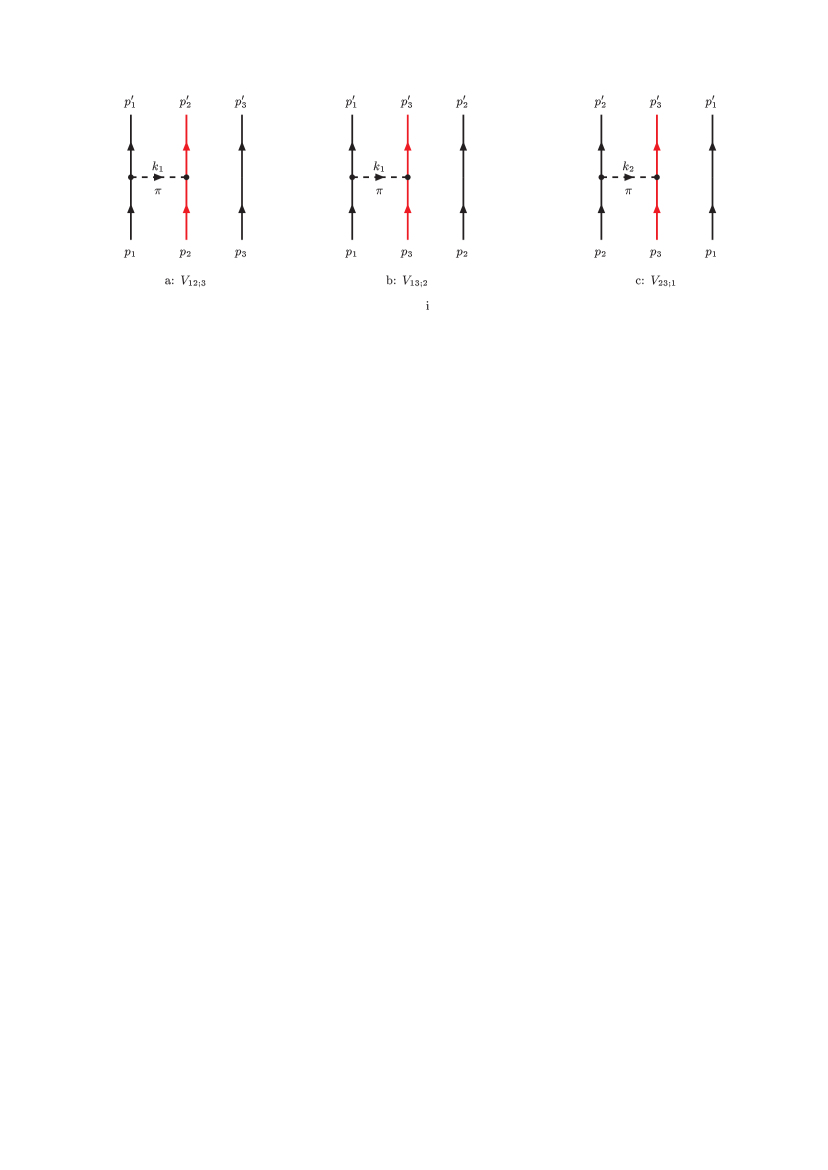
Figure 1: The Born-Feynman diagrams for two-body forces $V_{12;3},V_{13;2},V_{23;1}$

II A=3 Dalitz-Downs Model

II.1 Wave functions for the proton P(uud) and neutron N(udd)

The 3Q wave function is assumed to be of the following form Dal58 ; HT64 :

$$\psi_{3Q}(r_{1},r_{2},r_{3})=N_{3}\exp\left[-\frac{1}{2}\lambda\left({\bf x}_{12}^{2}+{\bf x}_{23}^{2}+{\bf x}_{31}^{2}\right)\right],$$ (1)

where ${\bf x}_{12}={\bf x}_{1}-{\bf x}_{2},\ {\bf x}_{23}={\bf x}_{2}-{\bf x}_{3},\ {\bf x}_{31}={\bf x}_{3}-{\bf x}_{1}.$ The Jacobian coordinates for the three-particle system are

$$\bm{\rho}=\frac{1}{\sqrt{2}}\left({\bf x}_{1}-{\bf x}_{2}\right)\hskip 28.45274pt \hskip 14.22636pt{\bf x}_{1}=\frac{1}{\sqrt{6}}\bm{\lambda}+\frac{1}{\sqrt{2}}\bm{\rho}+\frac{1}{\sqrt{3}}{\bf R},$$ , (2a)

$$\bm{\lambda}=\frac{1}{\sqrt{6}}\left({\bf x}_{1}+{\bf x}_{2}-2{\bf x}_{3}\right) \hskip 14.22636pt{\bf x}_{2}=\frac{1}{\sqrt{6}}\bm{\lambda}-\frac{1}{\sqrt{2}}\bm{\rho}+\frac{1}{\sqrt{3}}{\bf R},$$ , (2b)

$${\bf R}=\frac{1}{\sqrt{3}}\left({\bf x}_{1}+{\bf x}_{2}+{\bf x}_{3}\right)\hskip 2.84526pt \hskip 14.22636pt{\bf x}_{3}=-\sqrt{\frac{2}{3}}\bm{\lambda}+\frac{1}{\sqrt{3}}{\bf R}.$$ , (2c)

The differences expressed in the Jacobi-coordinates are

$${\bf x}_{1}-{\bf x}_{2}=\sqrt{2}\bm{\rho},\ \ {\bf x}_{1}-{\bf x}_{3}=\sqrt{\frac{1}{2}}\bm{\rho}+\sqrt{\frac{3}{2}}\bm{\lambda},$$

$${\bf x}_{2}-{\bf x}_{3}=-\sqrt{\frac{1}{2}}\bm{\rho}+\sqrt{\frac{3}{2}}\bm{\lambda},$$

which leads to the expression ${\bf x}_{12}^{2}+{\bf x}_{13}^{2}+{\bf x}_{23}^{2}=3\left(\bm{\rho}^{2}+\bm{\lambda}^{2}\right),$ and the three-nucleon wave function (1) becomes

$$\psi_{3Q}(r_{1},r_{2},r_{3})=N_{3}\exp\left[-\frac{3}{2}\lambda\left(\bm{\rho}^{2}+\bm{\lambda}^{2}\right)\right]\equiv\psi_{QN}(\bm{\rho},\bm{\lambda}).$$ (3)

The normalization is

$$1=\int d^{3}\rho\int d^{3}\lambda\ |\psi(\bm{\rho},\bm{\lambda})|^{2}=N_{3}^{2}\left(\frac{\pi}{3\lambda}\right)^{3}\rightarrow N_{3}=\left(\frac{3\lambda}{\pi}\right)^{3/2}.$$ (4)

II.2 Momentum-representation D&D model

1. Wave function: The momentum-space the 3Q-wave function is defined by

$$\widetilde{\psi}_{3Q}({\bf p}_{\rho},{\bf p}_{\lambda}) = N_{3}\int\int d^{3}\rho d^{3}\lambda\ e^{i\left({\bf p}_{\rho}\cdot\bm{\rho}+{\bf p}_{\lambda}\cdot\bm{\lambda}\right)}\exp\left[-\frac{3}{2}\lambda\left(\bm{\rho}^{2}+\bm{\lambda}^{2}\right)\right]$$ (5)

$$= \widetilde{N}_{3}\exp\left[-\frac{1}{6\lambda}\left({\bf p}_{\rho}^{2}+{\bf p}_{\lambda}^{2}\right)\right],\ \ {\rm with}\ \widetilde{N}_{3}=\left(\frac{4\pi}{3\lambda}\right)^{3/2},$$

and in configuration-space

$$\psi_{3Q}(\bm{\rho},\bm{\lambda})=\int\int\frac{d^{3}p_{\rho}}{(2\pi)^{3}}\frac{d^{3}p_{\lambda}}{(2\pi)^{3}}\ e^{-i\left({\bf p}_{\rho}\cdot\bm{\rho}+{\bf p}_{\lambda}\cdot\bm{\lambda}\right)}\ \widetilde{\psi}_{3Q}({\bf p}_{\rho},{\bf p}_{\lambda}),$$ (6)

and normalization

$$\int\int\frac{d^{3}p_{\rho}}{(2\pi)^{3}}\frac{d^{3}p_{\lambda}}{(2\pi)^{3}}|\widetilde{\psi}_{3Q}(\bm{p}_{\rho},{\bf p}_{\lambda})|^{2}=1.$$ (7)

Using the momentum-space wave functions of this subsection, given the momentum-space $\widetilde{V}_{3}$-potential, the integrals occurring in the matrix elements can executed analytically.

2. Momentum-space Matrix elements: We first translate the momenta that occur in the potentials in the $(\bm{\rho},\bm{\lambda})$-language. For the initial state the momenta are

$${\bf p}_{1}=\sqrt{\frac{1}{6}}{\bf p}_{\lambda}+\sqrt{\frac{1}{2}}{\bf p}_{\rho}+\sqrt{\frac{1}{3}}{\bf P},$$ (8a)

$${\bf p}_{2}=\sqrt{\frac{1}{6}}{\bf p}_{\lambda}-\sqrt{\frac{1}{2}}{\bf p}_{\rho}+\sqrt{\frac{1}{3}}{\bf P},$$ (8b)

$${\bf p}_{3}=-\sqrt{\frac{2}{3}}{\bf p}_{\lambda}+\sqrt{\frac{1}{3}}{\bf P},$$ (8c)

where $\sqrt{3}{\bf P}={\bf P}_{i}=\sum_{i=1}^{3}{\bf p}_{i}$, and similarly for the final state momenta. In passing we note that with these definitions

$$\sum_{i=1}^{3}{\bf p}_{i}\cdot{\bf x}_{i} = {\bf p}_{\rho}\cdot{\bf x}_{\rho}+{\bf p}_{\lambda}\cdot{\bf x}_{\lambda}+{\bf P}\cdot{\bf R}.$$

We work in the overall CM-momentum frame, i.e. for the total momentum in the initial and final state we have ${\bf P}={\bf P}_{f}=0$. Then, the customary momenta $({\bf q}_{i}=({\bf p}_{i}^{\prime}+{\bf p}_{i})/2$ and ${\bf k}_{i}={\bf p}_{i}^{\prime}-{\bf p}_{i}$ become in the $(\bm{\rho},\bm{\lambda})$-language

$${\bf k}_{1}=\frac{1}{\sqrt{6}}{\bf k}_{\lambda}+\frac{1}{\sqrt{2}}{\bf k}_{\rho} {\bf q}_{1}=\frac{1}{\sqrt{6}}{\bf q}_{\lambda}+\frac{1}{\sqrt{2}}{\bf q}_{\rho},$$ , (9a)

$${\bf k}_{2}=\frac{1}{\sqrt{6}}{\bf k}_{\lambda}-\frac{1}{\sqrt{2}}{\bf k}_{\rho} {\bf q}_{2}=\frac{1}{\sqrt{6}}{\bf q}_{\lambda}-\frac{1}{\sqrt{2}}{\bf q}_{\rho},$$ , (9b)

$${\bf k}_{3}=-\sqrt{\frac{2}{3}}{\bf k}_{\lambda}\hskip 28.45274pt {\bf q}_{3}=-\sqrt{\frac{2}{3}}{\bf q}_{\lambda}.$$ , (9c)

For the squares occurring in the wave functions and potentials we obtain

$${\bf p}_{\rho}^{\prime 2}+{\bf p}_{\rho}^{2}=2({\bf q}_{\rho}^{2}+\frac{1}{4}{\bf k}_{\rho}^{2}),\ \ {\bf p}_{\lambda}^{\prime 2}+{\bf p}_{\lambda}^{2}=2({\bf q}_{\lambda}^{2}+\frac{1}{4}{\bf k}_{\lambda}^{2}),$$ (10a)

$${\bf k}_{1}^{2}=\frac{1}{6}{\bf k}_{\lambda}^{2}+\frac{1}{2}{\bf k}_{\rho}^{2}+\frac{1}{\sqrt{3}}{\bf k}_{\rho}\cdot{\bf k}_{\lambda},$$ (10b)

$${\bf k}_{2}^{2}=\frac{1}{6}{\bf k}_{\lambda}^{2}+\frac{1}{2}{\bf k}_{\rho}^{2}-\frac{1}{\sqrt{3}}{\bf k}_{\rho}\cdot{\bf k}_{\lambda},$$ (10c)

$${\bf k}_{3}^{2}=\frac{2}{3}{\bf k}_{\lambda}^{2}.$$ (10d)

Working in the three-body CM-system, i.e. ${\bf P}=0$, the transformation between the different coordinates leads to

$$d^{3}p_{\rho}d^{3}p_{\lambda}d^{3}P=\left\|\begin{array}[]{ccc}\frac{\partial p_{\rho}}{\partial p_{1}}&\frac{\partial p_{\rho}}{\partial p_{2}}&\frac{\partial p_{\rho}}{\partial p_{3}}\\ \frac{\partial p_{\lambda}}{\partial p_{1}}&\frac{\partial p_{\lambda}}{\partial p_{2}}&\frac{\partial p_{\lambda}}{\partial p_{3}}\\ \frac{\partial P}{\partial p_{1}}&\frac{\partial P}{\partial p_{2}}&\frac{\partial P}{\partial p_{3}}\\ \end{array}\right\|\ d^{3}p_{1}d^{3}p_{2}d^{3}p_{3}=d^{3}p_{1}d^{3}p_{2}d^{3}p_{3},\ d^{3}p_{1}d^{3}p^{\prime}_{1}=d^{3}q_{1}d^{3}k_{1}.$$ (11)

In the case of a two-body interaction $V_{2}$ we take ${\bf k}_{3}=0$ and hence ${\bf k}_{2}=-{\bf k}_{1}\equiv{\bf k}$. In the case of the three-body interaction $V_{3}$ one has ${\bf k}_{1}+{\bf k}_{2}+{\bf k}_{3}=0$. With the setting of the Jacobi-coordinates in momentum space the matrix elements of the interactions can be evaluated using the momentum space representation of the potentials.

III V₂ Three-body matrix elements in Momentum Space

The three-body matrix element of the two-body potential $V_{2}$ is

$$\langle{\bf p}^{\prime}_{1},{\bf p}^{\prime}_{2},{\bf p}^{\prime}_{3}|V_{2}|{\bf p}_{1},{\bf p}_{2},{\bf p}_{3}\rangle=\langle{\bf p}^{\prime}_{1},{\bf p}^{\prime}_{2}|V_{2}|{\bf p}_{1},{\bf p}_{2}\rangle\cdot\langle{\bf p}^{\prime}_{3}|{\bf p}_{3}\rangle=$$

$$(2\pi)^{3}\ \langle{\bf p}^{\prime}_{1},{\bf p}^{\prime}_{2}|V_{2}|{\bf p}_{1},{\bf p}_{2}\rangle\cdot\delta^{3}({\bf p}^{\prime}_{3}-{\bf p}_{3})=$$

$$(2\pi)^{3}\ \delta^{3}({\bf p}_{1}^{\prime}+{\bf p}^{\prime}_{2}+{\bf p}^{\prime}_{3}-{\bf p}_{1}-{\bf p}_{2}-{\bf p}_{3})\cdot(2\pi)^{3}\langle{\bf p}^{\prime}_{1},{\bf p}^{\prime}_{2}|v_{2}|{\bf p}_{1},{\bf p}_{2}\rangle\cdot\delta^{3}({\bf p}^{\prime}_{3}-{\bf p}_{3}).$$ (12)

The factor $(2\pi)^{3}$ is due to the normalization of the one-particle momentum states, $({\bf p}^{\prime}|{\bf p})=(2\pi)^{3}\delta^{3}({\bf p}^{\prime}-{\bf p})$.
The $V_{2}$ interaction in momentum space for the central-, spin-spin-, tensor-, spin-orbit-, and quadratic-spin-orbit has factors: $1,{\bf k}^{2},{\bf q}^{2},{\bf k}\times{\bf q}$. We consider the $V_{12;3}$ potential. Then, for $V_{2}$ we have ${\bf k}_{2}=-{\bf k}_{1}$, and for the non-local potentials ${\bf q}^{2}\rightarrow({\bf q}_{1}^{2}+{\bf q}_{2}^{2})/2$. The evaluation of the three-body matrix elements using harmonic oscillator wave functions the overlap integrals $I_{3}(i,j)$ are given in this section.
In Appendix B we list a complete set of Gaussian integrals that enables to do all momentum space integrals relevant for this paper. Among them integrals quadratic in the components of the vectors ${\bf k}_{1}$ and ${\bf k}_{2}$. We define

$$H_{[k,l]}\equiv\langle\psi_{3}|\left({\bf k}^{2}\right)^{k}\left({\bf q}^{2}\right)^{l}\ G_{0}({\bf k}^{2};m^{2},\Lambda^{2})|\psi_{3}\rangle,\ \ {\rm with}$$ (13a)

$$G_{0}({\bf k}^{2};m^{2},\Lambda^{2})=e^{-{\bf k}^{2}/\Lambda^{2}}\ \bigl{[}{\bf k}^{2}+m^{2}\bigr{]}^{-1}.$$ (13b)

We also define the ”diffractive” matrix element by

$$D_{[k,l]}\equiv\langle\psi_{3}|\left({\bf k}^{2}\right)^{k}\left({\bf q}^{2}\right)^{l}\ G_{D}({\bf k}^{2};\Lambda^{2})|\psi_{3}\rangle,\ \ {\rm with}$$ (14a)

$$G_{D}({\bf k}^{2};\Lambda^{2})=e^{-{\bf k}^{2}/\Lambda^{2}}.$$ (14b)

a. Evaluation $V_{2}$ expectation values: For diagram (a) in Fig. 1 we evaluate in momentum space the basic integral

$$H_{[0,0]} = (2\pi)^{3}\widetilde{N}_{3}^{2}\ \int\frac{d^{3}p_{\rho}^{\prime}d^{3}p_{\lambda}^{\prime}}{(2\pi)^{6}}\int\frac{d^{3}p_{\rho}d^{3}p_{\lambda}}{(2\pi)^{6}}\left\{\exp\left[-\frac{1}{6\lambda}({\bf p}_{\rho}^{\prime 2}+{\bf p}_{\lambda}^{\prime 2})\right]\right.\cdot$$ (15)

$$\times\left.\exp\left[-\frac{1}{6\lambda}({\bf p}_{\rho}^{2}+{\bf p}_{\lambda}^{2})\right]\ \frac{e^{-{\bf k}^{2}/\Lambda^{2}}}{{\bf k}^{2}+m^{2}}\right\}$$

$$= (2\pi)^{-9}\widetilde{N}_{3}^{2}\ \int_{0}^{\infty}d\alpha\ e^{-\alpha m^{2}}\cdot\int d^{3}p_{\rho}^{\prime}d^{3}p_{\lambda}^{\prime}\int d^{3}p_{\rho}d^{3}p_{\lambda}\cdot$$

$$\times\left\{\exp\left[-\frac{1}{6\lambda}\left({\bf p}_{\rho}^{\prime 2}+{\bf p}_{\lambda}^{\prime 2}+{\bf p}_{\rho}^{2}+{\bf p}_{\lambda}^{2}\right)\right]\ e^{-\gamma{\bf k}^{2}}\right\},$$

where $\gamma=\alpha+\Lambda^{-2}$.

b. Cartesian momenta: Since the potentials $V_{2}$ are expressed in the cartesian momenta ${\bf k}_{i},(i=1,2,3)$ it is convenient to express the integral in (11) in terms of these variables. (This is also the case for the non-local momenta ${\bf q}_{i},(i=1,2,3)$ when the contribution of these terms is non-vanishing, of course.) In cartesian coordinates the exponential factor from the wave functions has

$${\bf p}_{\rho}^{\prime 2}+{\bf p}_{\lambda}^{\prime 2}+{\bf p}_{\rho}^{2}+{\bf p}_{\lambda}^{2}=4\biggl{[}({\bf q}_{1}^{2}+{\bf q}_{1}\cdot{\bf q}_{2}+{\bf q}_{2}^{2})+\frac{1}{4}({\bf k}_{1}^{2}+{\bf k}_{1}\cdot{\bf k}_{2}+{\bf k}_{2}^{2})\biggr{]}.$$ (16)

In cartesian momenta we get

$$H_{[0,0]}=(2\pi)^{-9}\ \widetilde{N}_{3}^{2}\ \int_{0}^{\infty}d\alpha\ e^{-\alpha m^{2}}\cdot\int d^{3}q_{1}d^{3}k_{1}\int d^{3}q_{2}d^{3}k_{2}\cdot$$

$$\times\exp\bigg{\{}-\frac{1}{6\lambda}\biggl{[}4({\bf q}_{1}^{2}+{\bf q}_{1}\cdot{\bf q}_{2}+{\bf q}_{2}^{2})+({\bf k}_{1}^{2}+{\bf k}_{1}\cdot{\bf k}_{2}+{\bf k}_{2}^{2})\biggr{]}\bigg{\}}\cdot e^{-\gamma{\bf k}^{2}}.$$ (17)

In Appendix A the details of the three-body matrix elements of $V_{2}$ are given, and below we summarize the results.

c. Resume: We rewrite the basic matrix element integral is (17) as follows:

$$H_{[0,0]} = {N}_{[0,0]}\int_{0}^{\infty}d\alpha\ e^{-\alpha m^{2}}\cdot\int d^{3}q_{1}d^{3}k_{1}\int d^{3}q_{2}d^{3}k_{2}\cdot$$ (18)

$$\times\exp\bigg{\{}-\frac{1}{6\lambda}\biggl{[}4({\bf q}_{1}^{2}+{\bf q}_{1}\cdot{\bf q}_{2}+{\bf q}_{2}^{2})+({\bf k}_{1}^{2}+{\bf k}_{1}\cdot{\bf k}_{2}+{\bf k}_{2}^{2})\biggr{]}\bigg{\}}\cdot e^{-\gamma{\bf k}^{2}}$$

$$\equiv \int_{0}^{\infty}d\alpha\ e^{-\alpha m^{2}}\ F_{[0,0]}(\alpha,\beta,\gamma),$$

where $N_{[0,0]}=(2\pi)^{-9}\widetilde{N}_{3}^{2}$, and $\beta=1/6\lambda,\gamma=\alpha+1/\Lambda^{2}$. Then,

$$F_{[0,0]}(\alpha,\beta,\gamma)=N_{[0,0]}\int d^{3}q_{1}d^{3}k_{1}\int d^{3}q_{2}d^{3}k_{2}\ e^{-\gamma{\bf k}^{2}}\cdot$$

$$\times\exp\bigg{\{}-\frac{1}{6\lambda}\biggl{[}4({\bf q}_{1}^{2}+{\bf q}_{1}\cdot{\bf q}_{2}+{\bf q}_{2}^{2})+({\bf k}_{1}^{2}+{\bf k}_{1}\cdot{\bf k}_{2}+{\bf k}_{2}^{2})\biggr{]}\bigg{\}}=N_{[0,0]}\cdot$$

$$\times\left(\frac{\pi^{2}}{12\beta^{2}}\right)^{3/2}\ \left(\frac{\pi}{\beta+\gamma}\right)^{3/2}=(2\pi)^{-6}\left(\frac{16\pi}{3}\right)^{3/2}\ \Lambda^{3}\left(1+\frac{\Lambda^{2}R_{N}^{2}}{18}+\frac{\Lambda^{2}}{m^{2}}\ \bar{\alpha}\right)^{-3/2}.$$ (19)

with $\bar{\alpha}=\alpha m^{2}$. For $H_{[m,n]}$ we have

$$F_{[2,0]} = \frac{3}{2}(\beta+\gamma)^{-1}\ F_{[0,0]}=\frac{3}{2}\Lambda^{2}\ \left(1+\frac{\Lambda^{2}R_{N}^{2}}{18}+\frac{\Lambda^{2}}{m^{2}}\ \bar{\alpha}\right)^{-1}\ F_{[0,0]},$$ (20a)

$$F_{[4,0]} = \frac{15}{4}(\beta+\gamma)^{-2}\ F_{[0,0]}=\frac{15}{4}\Lambda^{4}\ \left(1+\frac{\Lambda^{2}R_{N}^{2}}{18}+\frac{\Lambda^{2}}{m^{2}}\ \bar{\alpha}\right)^{-2}\ F_{[0,0]},$$ (20b)

$$F_{[0,2]} = \frac{1}{3\beta}\ F_{[0,0]}=6\Lambda^{2}\ (\Lambda R_{N})^{-2}\ F_{[0,0]},$$ (20c)

$$F_{[2,2]} = \frac{1}{2\beta}(\beta+\gamma)^{-1}\ F_{[0,0]}=9\Lambda^{4}\ (\Lambda R_{N})^{-2}\ \left(1+\frac{\Lambda^{2}R_{N}^{2}}{18}+\frac{\Lambda^{2}}{m^{2}}\ \bar{\alpha}\right)^{-1}\$$ (20d)

The tensor operator matrix element has a factor $-k_{i}k_{j}$, which gives

$$F^{T}_{i,j}([0,0]) = -[2(\beta+\gamma)]^{-1}\ F_{[0,0]}\ \delta_{ij}=-\frac{1}{2}\Lambda^{2}\left(1+\frac{\Lambda^{2}R_{N}^{2}}{18}+\frac{\Lambda^{2}}{m^{2}}\ \bar{\alpha}\right)^{-1}\ F_{[0,0]}\ \delta_{ij}.$$ (21)

The quadratic spin-orbit operator matrix element has a factor $-k_{i}k_{j}q_{m}q_{n}$, which gives

$$F^{Q}_{i,m;j,n}([0,0]) = [6\beta(\beta+\gamma)]^{-1}\ F_{[0,0]}\ \delta_{i,j}\delta_{m,n}=3\Lambda^{4}(\Lambda R_{N})^{-2}\left(1+\frac{\Lambda^{2}R_{N}^{2}}{18}+\frac{\Lambda^{2}}{m^{2}}\ \bar{\alpha}\right)^{-1}\cdot$$ (22)

$$\times F_{[0,0]}\ \delta_{i,j}\delta_{m,n}.$$

For the $G_{[n,m]}$ functions the correspondent $F_{[n,m]}$ are the same as those above, but with $\bar{\alpha}=0$.

d. Explicit expressions: From Appendix A we obtain for $H_{[0,0]}$, the expression

$$H_{[0,0]}={\cal N}_{[0,0]}\int_{0}^{\infty}d\alpha\ e^{-\alpha m^{2}}\ \left(\frac{\pi}{\alpha+A}\right)^{3/2}\ ,\ A=\left(1+\frac{\Lambda^{2}R_{N}^{2}}{18}\right)/\Lambda^{2},$$ (23)

where ${\cal N}_{[0,0]}=(3\pi^{2}\lambda^{2})^{3/2}N_{[0,0]}$. The $\alpha$-integral, called $J_{1}$ (97), is worked out in Appendix A with the result

$$H_{[0,0]}=(2\pi\sqrt{\pi})\ {\cal N}_{[0,0]}\ m\ \biggl{[}\frac{1}{\sqrt{\pi Am^{2}}}-e^{Am^{2}}\ {\it Erfc}\left(\sqrt{Am^{2}}\right)\biggr{]}.$$ (24)

Also, $G_{[0,0]}=F_{[0,0]}(\alpha=0,\beta,\gamma)=\pi\ {\cal N}_{[0,0]}\ A^{-3/2}$. For $H_{[2,0]}$ the integral expression is

$$H_{[2,0]}=(3/2\pi)\ {\cal N}_{[0,0]}\int_{0}^{\infty}d\alpha\ e^{-\alpha m^{2}}\ \left(\frac{\pi}{\alpha+A}\right)^{5/2},$$ (25)

which, using the $J_{2}$-integral (114),

$$H_{[2,0]}=(2\pi\sqrt{\pi})\ {\cal N}_{[0,0]}\ m^{3}\ \biggl{[}e^{Am^{2}}\ {\it Erfc}\left(\sqrt{Am^{2}}\right)+\frac{1}{2\sqrt{\pi}}(Am^{2})^{-3/2}\left(1-2Am^{2}\right)\biggr{]},$$ (26)

with the relation $H_{[2,0]}=G_{[0,0]}-m^{2}H_{[0,0]}$ (check!).

For the presentation of the QQ-potential contributions to the nucleon mass it is useful to introduce the dimensionless $B_{[k,l]}$ as follows

$$H_{[0,0]}=m\ B_{[0,0]},\ H_{[2,0]}=m^{3}\ B_{[2,0]},H_{[0,2]}=m^{3}\ B_{[0,2]},\ H_{[2,2]}=m^{5}\ B_{[2,2]}.$$ (27)

Similarly, for the Pomeron we define

$$G_{[0,0]}=\frac{\Lambda^{3}}{{\cal M}^{2}}\ D_{[0,0]},\ G_{[2,0]}=\frac{\Lambda^{5}}{{\cal M}^{2}}m^{3}\ D_{[2,0]},G_{[0,2]}=\frac{\Lambda^{5}}{{\cal M}^{2}}\ D_{[0,2]}.$$ (28)

Remark: The tensor-integral gives a $\delta_{ij}$ factor. Contraction with $\sigma_{1,i}\sigma_{2,j}-(1/3)(\bm{\sigma}_{1}\cdot\bm{\sigma}_{2})\ \delta_{i,j}$ gives zero. Therefore, for s-wave quarks the tensor-potential gives no contribution, which is logical.

 

IV Kinetic Energy Three-quark System

1. Quark-contribution: For equal quark masses $m_{i}=m_{Q}\ (i=1,2,3)$ the non-relativistic kinetic energy operator is kin-energy

$$T_{op}=\left[{\bf p}_{1}^{2}+{\bf p}_{2}^{2}+{\bf p}_{3}^{2}\right]/(2m_{Q})=\frac{1}{2m_{Q}}\left[{\bf p}_{\lambda}^{2}+{\bf p}_{\rho}^{2}\right].$$ (29)

Then,

$$T = \langle\Psi_{3}|T_{op}|\Psi_{3}\rangle=\Pi_{i=1}^{3}\biggl{[}\int\frac{d^{3}p_{i}}{(2\pi)^{3}}\biggr{]}\ \Psi^{*}({\bf p}_{i})\ \left[{\bf p}_{1}^{2}+{\bf p}_{2}^{2}+{\bf p}_{3}^{2}\right]/(2m_{Q})\Psi({\bf p}_{i})$$ (30)

$$= \widetilde{N}_{3}^{2}\ \int\int\frac{d^{3}p_{\lambda}d^{3}p_{\rho}}{(2\pi)^{6}}\ \exp\biggl{[}-\frac{1}{3\lambda}\left({\bf p}_{\lambda}^{2}+{\bf p}_{\rho}^{2}\right)\biggr{]}\ \left({\bf p}_{\lambda}^{2}+{\bf p}_{\rho}^{2}\right)/(2m_{Q})=\widetilde{N}_{3}^{2}\cdot$$

$$\times (2\pi)^{-6}(3\pi\lambda)^{3/2}\ \frac{3}{2\pi}(3\pi\lambda)^{5/2}/m_{Q}=9\lambda/(2m_{Q})=(27/2)(m_{Q}R_{N})^{-2}\ m_{Q}.$$

Here is used $\widetilde{N}_{3}=(4\pi/3\lambda)^{3/2}$ and $\lambda=3R_{N}^{-2}$. With $R_{N}=1$ fm and $m_{Q}$=312.75 MeV one gets $\langle T\rangle\approx(9/2)m_{Q}$ which implies per quark a kinetic energy $\approx 470$ MeV. Clearly the quarks move relativistically, and the non-relativistic formula is wrong.

2. de Broglie estimation: An alternative derivation is as follows: Using the de Broglie relation between momentum and wave-length $p=h/\lambda$, one has for each quark

$$pc\approx 2\pi\ \frac{\hbar c}{2R_{N}}\rightarrow\frac{{\bf p}^{2}}{2m_{Q}}\approx\frac{\pi^{2}}{2}\frac{(\hbar c)^{2}}{m_{Q}R_{N}^{2}}=\frac{\pi^{2}}{2}\frac{(\hbar c)^{2}}{(m_{Q}R_{N})^{2}}\ m_{Q}.$$ (31)

With $\hbar c=197.325$ MeVfm we obtain for $R_{N}=1$ fm the kinetic energy per quark $1.6m_{Q}=500$ MeV, which agrees roughly with the more exact result in (30).
3. Relativistic Energy Expectation-value: First we derive a gaussian-type of presentation for the relativistic energy. Using integral representations, see TAR91 , we derive for the relativistic energy a gaussian-type of expression

$$E({\bf p}) = \sqrt{{\bf p}^{2}+m^{2}}=\frac{{\bf p}^{2}+m^{2}}{\sqrt{{\bf p}^{2}+m^{2}}}=\frac{2}{\pi}\int_{0}^{\infty}d\lambda\ \frac{{\bf p}^{2}+m^{2}}{{\bf p}^{2}+m^{2}+\lambda^{2}}$$ (32)

$$= ({\bf p}^{2}+m^{2})\cdot\frac{2}{\pi}\int_{0}^{\infty}d\lambda\ \int_{0}^{\infty}d\alpha\ \exp\bigl{[}-\alpha({\bf p}^{2}+m^{2}+\lambda^{2})\bigr{]}$$

$$= ({\bf p}^{2}+m^{2})\cdot\frac{1}{\sqrt{\pi}}\int_{0}^{\infty}\frac{d\alpha}{\sqrt{\alpha}}\ e^{-\alpha m^{2}}\ e^{-\alpha{\bf p}^{2}}.$$

Then, the expression for the relativistic kinetic energy of the three-quark system becomes

$$E_{T} = \bigl{\langle}\sum_{i=1}^{3}\sqrt{{\bf p}_{i}^{2}+m^{2}}\bigr{\rangle}=\frac{1}{\sqrt{\pi}}\int_{0}^{\infty}\frac{d\alpha}{\sqrt{\alpha}}e^{-\alpha m^{2}}\ \bigl{\langle}\sum_{i=1}^{3}({\bf p}_{i}^{2}+m^{2})\ e^{-\alpha{\bf p}_{i}^{2}}\bigr{\rangle}.$$ (33)

The evaluation of the expectation value in (33) involves only gaussian integrals and is straightforward. We remind the formulas, with ${\bf P}=0$,

$${\bf p}_{1}^{2} = \frac{1}{6}{\bf p}_{\lambda}^{2}+\frac{1}{2}{\bf p}_{\rho}^{2}+\frac{1}{\sqrt{3}}{\bf p}_{\lambda}\cdot{\bf p}_{\rho},$$

$${\bf p}_{2}^{2} = \frac{1}{6}{\bf p}_{\lambda}^{2}+\frac{1}{2}{\bf p}_{\rho}^{2}-\frac{1}{\sqrt{3}}{\bf p}_{\lambda}\cdot{\bf p}_{\rho},$$

$${\bf p}_{3}^{2} = ({\bf p}_{1}+{\bf p}_{2})^{2}=\frac{2}{3}{\bf p}_{\lambda}^{2}.$$

(a) For quark 1 the expectation of the kinetic energy is given by

$$\bigl{\langle}E_{T}\bigr{\rangle}_{1} = \biggl{\langle}\Psi\bigg{|}\frac{1}{\sqrt{\pi}}\int_{0}^{\infty}\frac{d\alpha}{\sqrt{\alpha}}\ e^{-\alpha m^{2}}\ ({\bf p}_{1}^{2}+m^{2})\ e^{-\alpha{\bf p}_{1}^{2}}\big{|}\Psi\biggr{\rangle}=\frac{1}{\sqrt{\pi}}\int_{0}^{\infty}\frac{d\alpha}{\sqrt{\alpha}}\ e^{-\alpha m^{2}}\cdot$$ (34)

$$\times\bigg{\{}\ \widetilde{N}_{3}^{2}\int\frac{d^{3}p_{\lambda}d^{3}p_{\rho}}{(2\pi)^{6}}\ \exp\left[-\frac{1}{3\lambda}({\bf p}_{\lambda}^{2}+{\bf p}_{\rho}^{2})\right]\ ({\bf p}_{1}^{2}+m^{2})\ e^{-\alpha{\bf p}_{1}^{2}}\biggr{\}}$$

The momentum integral $I\equiv\bigl{\{}\ldots\bigr{\}}$ is

$$I = \biggl{(}-\frac{d}{d\alpha}+m^{2}\biggr{)}\ \widetilde{N}_{3}^{2}\int\frac{d^{3}p_{\lambda}d^{3}p_{\rho}}{(2\pi)^{6}}\ \exp\biggl{[}-\biggl{(}\frac{1}{3\lambda}\left[{\bf p}_{\lambda}^{2}+{\bf p}_{\rho}^{2}\right]\$$ (35)

$$+\alpha\left[\frac{1}{6}{\bf p}_{\lambda}^{2}+\frac{1}{2}{\bf p}_{\rho}^{2}+\frac{1}{\sqrt{3}}{\bf p}_{\lambda}\cdot{\bf p}_{\rho}\right]\biggr{)}\biggr{]}\equiv\left(-\frac{d}{d\alpha}+m^{2}\right)\ J$$

where

$$J = \widetilde{N}_{3}^{2}\int\frac{d^{3}p_{\lambda}d^{3}p_{\rho}}{(2\pi)^{6}}\ \exp\bigg{[}-\bigl{\{}a{\bf p}_{\lambda}^{2}+c{\bf p}_{\lambda}\cdot{\bf p}_{\rho}+b{\bf p}_{\rho}^{2}\bigr{\}}\bigg{]},\ \rm{where}$$ (36a)

$$a = \frac{1}{3\lambda}+\frac{\alpha}{6}\ ,\ b=\frac{1}{3\lambda}+\frac{\alpha}{2}\ ,\ c=\frac{\alpha}{\sqrt{3}}.$$ (36b)

From the integrals in Eqn. (124f) we have

$$J(a,b,c) = \widetilde{N}_{3}^{2}(2\pi)^{-6}\left(\frac{4\pi^{2}}{4ab-c^{2}}\right)^{3/2}=(1+2\lambda\alpha)^{-3/2},\ -\frac{d}{d\alpha}J(a,b,c)=3\lambda\left(1+2\lambda\alpha\right)^{-5/2}.$$ (37)

The integral in (35) becomes

$$I(\alpha,\lambda) = \bigl{(}1+2\alpha\lambda\bigr{)}^{-3/2}\biggl{[}m^{2}+3\lambda\bigl{(}1+2\alpha\lambda\biggr{)}^{-1}\biggr{]}$$ (38)

$$= m^{2}\left(1+6\frac{\alpha m^{2}}{m^{2}R_{N}^{2}}\right)^{-3/2}\biggl{[}1+9(mR_{N})^{-2}\ \left(1+6\frac{\alpha m^{2}}{m^{2}R_{N}^{2}}\right)^{-1}\biggr{]}.$$

Because of the symmetry, the total kinetic energy is three times that for quark 1, so

$$\bigg{\langle}E_{T}\biggr{\rangle} = \frac{3m^{2}}{\sqrt{\pi}}\int_{0}^{\infty}\frac{d\alpha}{\sqrt{\alpha}}\ e^{-\alpha m^{2}}\biggl{[}\left(1+6\frac{\alpha m^{2}}{m^{2}R_{N}^{2}}\right)^{-3/2}+9(mR_{N})^{-2}\ \left(1+6\frac{\alpha m^{2}}{m^{2}R_{N}^{2}}\right)^{-5/2}\biggr{]}$$ (39)

$$= \frac{6m}{\sqrt{\pi}}\int_{0}^{\infty}dy\ e^{-y^{2}}\biggl{[}\biggl{(}1+\frac{6y^{2}}{m^{2}R_{N}^{2}}\biggr{)}^{-3/2}+9(mR_{N})^{-2}\biggl{(}1+\frac{6y^{2}}{m^{2}R_{N}^{2}}\biggr{)}^{-5/2}\biggr{]}.$$

We remark that

$$\lim_{R_{N}\rightarrow\infty}E_{T}=\frac{3m}{\sqrt{\pi}}\int_{0}^{\infty}\frac{d\alpha}{\sqrt{\alpha}}\ e^{-\alpha m^{2}}=\frac{6m}{\sqrt{\pi}}\int_{0}^{\infty}dy\ e^{-y^{2}}=3m.$$

In a concise form we write

$$E_{T}(mR_{N}) = \frac{1}{\sqrt{6}}(mR_{N})^{3}\ \biggl{[}K_{3}+\frac{3}{2}K_{5}\biggr{]}\ m,\ T_{rel}=E_{T}-3m,$$ (40a)

$$K_{n}(mR_{N}) = \frac{1}{\sqrt{\pi}}\int_{0}^{\infty}dy\ e^{-y^{2}}\ \left(y^{2}+d^{2}\right)^{-n/2}\ {\rm with}\ d=mR_{N}/\sqrt{6}.$$ (40b)

In Table 1 the numerical results are shown for the kinetic energies (K.E.’s) as a function of the radius $R_{N}$.

Table 1: Kinetic energy $E_{T}$ as a function of $R_{N}$. Listed are the integrals $K_{3,5}$, the non-relativistic K.E. $T_{NR}$ and the relativistic K.E. $T_{R}$ per quark.

$R_{N}$[fm]	$\bigl{\langle}p\bigr{\rangle}$	$K_{3}$	$K_{5}$	$T_{NR}(1Q)$	$T_{R}(1Q)$	$T_{R}(3Q)$
0.50	519.4	8.37	57.66	2241.0	820.8	2462.5
0.60	432.8	5.62	27.45	1556.2	653.6	1960.9
0.70	371.0	3.99	14.60	1143.4	536.1	1608.3
0.80	324.6	2.94	8.40	875.4	448.4	1345.2
0.90	288.6	2.24	5.14	691.7	380,8	1142.5
1.00	259.7	1.75	3.30	560.2	327.6	982.9
1.20	216.4	1.13	1.52	389.1	250.2	750.7
1.40	185.5	0.77	0.78	285.8	197.6	592.8
1.60	162.3	0.55	0.44	218.8	160.0	480.0
1.80	144.3	0.41	0.26	172.9	132.2	396.6
2.00	130.0	0.31	0.163	140.1	111.0	333.0

4. Average quark momentum: The expectation value for ${\bf p}_{1}^{2}$ is given by

$$\bigl{\langle}{\bf p}_{1}^{2}\bigr{\rangle} = \widetilde{N}_{3}^{2}\int\frac{d^{3}p_{\lambda}d^{3}p_{\rho}}{(2\pi)^{6}}\ {\bf p}_{1}^{2}\ \exp\left[-\frac{1}{3\lambda}({\bf p}_{\lambda}^{2}+{\bf p}_{\rho}^{2})\right]$$ (41)

$$= \widetilde{N}_{3}^{2}\int\frac{d^{3}p_{1}d^{3}p_{2}}{(2\pi)^{6}}\ {\bf p}_{1}^{2}\ \exp\bigg{[}-\left(a{\bf p}_{1}^{2}+b{\bf p}_{2}^{2}+c{\bf p}_{1}\cdot{\bf p}_{2}\right)\biggr{]}$$

$$= \widetilde{N}_{3}^{2}\ (2\pi)^{-6}\ \frac{3b}{2\pi^{2}}\ \left(\frac{4\pi^{2}}{4ab-c^{2}}\right)^{5/2}=\sqrt{3}\ R_{N}^{-2}.$$

So, the average quark momentum is $\langle p\rangle=3^{1/4}\ R_{N}^{-1}$. The average K.E. $\langle T(1Q)\rangle=(\langle p\rangle)^{2}/2m_{Q}$ matches with $T_{NR}(1Q)$ in Table 1. The average relativistic energy is $E_{av}=\sqrt{p_{av}^{2}+m_{Q}^{2}}$, Defining the average quark mass by $m_{av}=(E_{av}+m_{Q})/2$ gives for $R_{N}=1$ fm a value $m_{av}=469=1.5m_{Q}$ MeV. Since the quarks are relativistic it is better in the QQ-potentials to make the replacements $1/(4m_{q}^{2})\rightarrow 1/(4m_{av}^{2})$, which gives for the the tensor, spin-orbit a reduction by a factor $\approx 6$, and for the quadratic spin-orbit a reduction by $\approx 39$. This makes these potential more reasonable, without having to do a fully relativistic calculation. In Appendix H a more exact, but rather complicated, way of including relativistic effects is described.

5. CM subtraction: Considering the 3-quark system residing in a central harmonic confining potential we subtract the zero-mode energy from the kinetic energy (?!). With

$$V_{conf}=C_{2}\ r_{N}^{2}=\frac{1}{2}m_{N}\omega_{CM}^{2}\ {\bf r}_{N}^{2}$$ (42)

one has

$$E_{CM}=\frac{3}{2}\hbar\ \omega_{CM},\ {\rm with}\ \omega_{CM}=\sqrt{\frac{2C_{2}}{3m_{Q}}}.$$ (43)

Using $C_{2}=315$ MeV fm^-2 and $m_{Q}=M_{p}/3$ one obtains $E_{CM}\approx 231$ MeV.

 

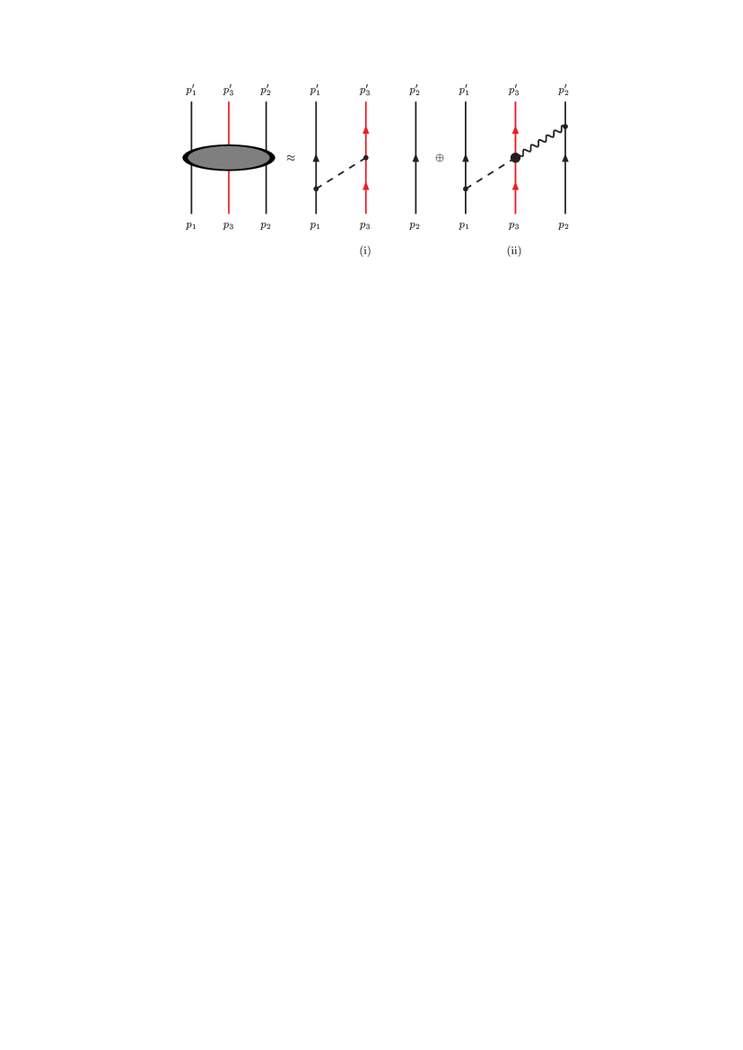
Figure 2: Three-particle amplitude (a) and the Born-Feynman graphs type (i) and (ii)

 

V Nucleon Mass from Two-body forces

In this note we calculate the contribution to the nucleon-mass from the two-body QQ-potentials, see graph (i) in Fig. 2. The contributions from the three-body QQQ-potentials, see graph (ii) in Fig. 2, will be derived in another note THAR.3bf .
Here, explicit formulas are given for the contributions to the nucleon-energy, i.e. nucleon mass, from the two-body QQ-potentials. The formulas below are based on the potentials in section D. Below, the contributions from the local, non-local, and ”additional” potentials are listed separately. (”Additional” = contributions to potentials due to the extra meson-quark-quark vertices, which have been introduced in order to match with the potentials at the baryon-level.)

Below we compute the contributions from the potentials for the graphs (a)-(c) of Fig. 1 to the expectation values $E_{N}=\langle\Psi_{N}|V_{2}|\Psi_{N}\rangle$ for the different OBE-potentials. The $V_{13;2}$ and $V_{23;1}$ give identical results in the case of the nucleon. Therefore, we multiply the results for $V_{12;3}$ by a factor 3 to obtain the total answer.
We remark that terms proportional to ${\bf q}_{i}$ and/or ${\bf k}_{i}$ vanish due to the integrations in the matrix elements $\langle\Psi_{3Q}|V_{2}|\Psi_{3Q}\rangle$, which implies no contributions from the spin-orbit potentials. This is logical because of the absence of P-waves etc. in the quark wave functions.

 

1. Nucleon: The isospin-spin operators that occur in $E_{N}$ are $\bm{\tau}_{1}\cdot\bm{\tau}_{2}$, $\bm{\sigma}_{1}\cdot\bm{\sigma}_{2}$, and the product $\bm{\tau}_{1}\cdot\bm{\tau}_{2}\ \bm{\sigma}_{1}\cdot\bm{\sigma}_{2}$. The symmetrized spin-isospin part of the nucleon state is

$$\Psi_{N} = \frac{1}{\sqrt{2}}\left(\vphantom{\frac{A}{A}}\phi_{M,S}\chi_{M,S}+\phi_{M,A}\chi_{M,A}\right).$$ (44)

In Appendix F the nucleon matrix elements of the spin-isospin operators are derived, with the result, see (177):

$$\left(\Psi_{N}|\bm{\tau}_{1}\cdot\bm{\tau}_{2}|\Psi_{N}\right)=\left(\Psi_{N}|\bm{\tau}_{1}\cdot\bm{\tau}_{3}|\Psi_{N}\right)=\left(\Psi_{N}|\bm{\tau}_{2}\cdot\bm{\tau}_{3}|\Psi_{N}\right)=-1,$$ (45a)

$$\left(\Psi_{N}|\bm{\sigma}_{1}\cdot\bm{\sigma}_{2}|\Psi_{N}\right)=\left(\Psi_{N}|\bm{\sigma}_{1}\cdot\bm{\sigma}_{3}|\Psi_{N}\right)=\left(\Psi_{N}|\bm{\sigma}_{2}\cdot\bm{\sigma}_{3}|\Psi_{N}\right)=-1,$$ (45b)

$$\left(\Psi_{N}|\bm{\tau}_{1}\cdot\bm{\tau}_{2}\ \bm{\sigma}_{1}\cdot\bm{\sigma}_{2}|\Psi_{N}\right)=\left(\Psi_{N}|\bm{\tau}_{1}\cdot\bm{\tau}_{3}\ \bm{\sigma}_{1}\cdot\bm{\sigma}_{3}|\Psi_{N}\right)=$$

$$\left(\Psi_{N}|\bm{\tau}_{2}\cdot\bm{\tau}_{3}\ \bm{\sigma}_{2}\cdot\bm{\sigma}_{3}|\Psi_{N}\right)=+5.$$ (45c)

The antisymmetry of the full nucleon state is provided by the color part of the wave function being the singlet $SU(3)_{c}$-irrep.

Here, including a factor 3 takes into account of the similar contributions from $V_{13;2}$ and $V_{23;1}$.

2. $\bm{\Lambda}$: For the $\Lambda$ the spin-isospin matrix elements are, see (177),

$$\left(\Psi_{\Lambda}|\bm{\tau}_{1}\cdot\bm{\tau}_{2}|\Psi_{\Lambda}\right)=\left(\Psi_{\Lambda}|\bm{\tau}_{1}\cdot\bm{\tau}_{3}|\Psi_{\Lambda}\right)=\left(\Psi_{\Lambda}|\bm{\tau}_{2}\cdot\bm{\tau}_{3}|\Psi_{\Lambda}\right)=-1,$$ (46a)

$$\left(\Psi_{\Lambda}|\bm{\sigma}_{1}\cdot\bm{\sigma}_{2}|\Psi_{\Lambda}\right)=\left(\Psi_{\Lambda}|\bm{\sigma}_{1}\cdot\bm{\sigma}_{3}|\Psi_{\Lambda}\right)=\left(\Psi_{\Lambda}|\bm{\sigma}_{2}\cdot\bm{\sigma}_{3}|\Psi_{\Lambda}\right)=-1,$$ (46b)

$$\left(\Psi_{\Lambda}|\bm{\tau}_{1}\cdot\bm{\tau}_{2}\ \bm{\sigma}_{1}\cdot\bm{\sigma}_{2}|\Psi_{\Lambda}\right)=\left(\Psi_{\Lambda}|\bm{\tau}_{1}\cdot\bm{\tau}_{3}\ \bm{\sigma}_{1}\cdot\bm{\sigma}_{3}|\Psi_{\Lambda}\right)=$$

$$\left(\Psi_{\Lambda}|\bm{\tau}_{2}\cdot\bm{\tau}_{3}\ \bm{\sigma}_{2}\cdot\bm{\sigma}_{3}|\Psi_{\Lambda}\right)=+2.$$ (46c)

The total three-body matrix element has three terms $\langle V_{2}\rangle=\langle V_{12;3}\rangle+\langle V_{13;2}\rangle+\langle V_{23;1}\rangle$, where $V_{12;3}=V_{UD}(12),V_{13;2}=V_{US}(13),V_{23;1}=V_{DS}(23)$.

3. $\bm{\Sigma^{+}}$: The wave functions for $\Psi_{\Sigma^{+}}$ is

$$\phi_{M,S}=\frac{1}{\sqrt{6}}\biggl{[}(us+su)u-2uus\biggr{]},\ \phi_{M,A}=\frac{1}{\sqrt{2}}(us-su)u,$$

and for for the spin wave functions $\chi_{M,S}$ and $\chi_{M,A}$ similarly as for the proton P. This gives, see (176),

$$\left(\Psi_{\Sigma}|\bm{\tau}_{1}\cdot\bm{\tau}_{2}|\Psi_{\Sigma}\right)=-\frac{1}{6}\ ,\ \left(\Psi_{\Sigma}|\bm{\tau}_{1}\cdot\bm{\tau}_{3}|\Psi_{\Sigma}\right)=\left(\Psi_{\Sigma}|\bm{\tau}_{2}\cdot\bm{\tau}_{3}|\Psi_{\Sigma}\right)=+\frac{2}{3},$$ (47a)

$$\left(\Psi_{\Sigma}|\bm{\sigma}_{1}\cdot\bm{\sigma}_{2}|\Psi_{\Sigma}\right)=\left(\Psi_{\Sigma}|\bm{\sigma}_{1}\cdot\bm{\sigma}_{3}|\Psi_{\Sigma}\right)=\left(\Psi_{\Sigma}|\bm{\sigma}_{2}\cdot\bm{\sigma}_{3}|\Psi_{\Sigma}\right)=-1,$$ (47b)

$$\left(\Psi_{\Sigma}|\bm{\tau}_{1}\cdot\bm{\tau}_{2}\ \bm{\sigma}_{1}\cdot\bm{\sigma}_{2}|\Psi_{\Sigma}\right)=-\frac{1}{6}\ ,\ \left(\Psi_{\Sigma}|\bm{\tau}_{1}\cdot\bm{\tau}_{3}\ \bm{\sigma}_{1}\cdot\bm{\sigma}_{3}|\Psi_{\Sigma}\right)=+\frac{1}{3}\ ,\$$

$$\left(\Psi_{\Sigma}|\bm{\tau}_{2}\cdot\bm{\tau}_{3}\ \bm{\sigma}_{2}\cdot\bm{\sigma}_{3}|\Psi_{\Sigma}\right)=+\frac{1}{3}.$$ (47c)

The total three-body matrix element has three terms $\langle V_{2}\rangle=\langle V_{12;3}\rangle+\langle V_{13;2}\rangle+\langle V_{23;1}\rangle$, where $V_{12;3}=V_{U}D(12),V_{13;2}=V_{U}S(13),V_{23;1}=V_{DS}(23)$.

4. $\bm{\Xi^{0}}$: In this case the matrix elements are, see (184),

$$\left(\Psi_{\Xi}|\bm{\tau}_{1}\cdot\bm{\tau}_{2}|\Psi_{\Xi}\right)=\left(\Psi_{\Xi}|\bm{\tau}_{1}\cdot\bm{\tau}_{3}|\Psi_{\Xi}\right)=\left(\Psi_{\Xi}|\bm{\tau}_{2}\cdot\bm{\tau}_{3}|\Psi_{\Xi}\right)=0,$$ (48a)

$$\left(\Psi_{\Xi}|\bm{\sigma}_{1}\cdot\bm{\sigma}_{2}|\Psi_{\Xi}\right)=\left(\Psi_{\Xi}|\bm{\sigma}_{1}\cdot\bm{\sigma}_{3}|\Psi_{\Xi}\right)=\left(\Psi_{\Xi}|\bm{\sigma}_{2}\cdot\bm{\sigma}_{3}|\Psi_{\Xi}\right)=-1,$$ (48b)

$$\left(\Psi_{\Xi}|\bm{\tau}_{1}\cdot\bm{\tau}_{2}\ \bm{\sigma}_{1}\cdot\bm{\sigma}_{2}|\Psi_{\Xi}\right)=\left(\Psi_{\Xi}|\bm{\tau}_{1}\cdot\bm{\tau}_{3}\ \bm{\sigma}_{1}\cdot\bm{\sigma}_{3}|\Psi_{\Xi}\right)=$$

$$\left(\Psi_{\Xi}|\bm{\tau}_{2}\cdot\bm{\tau}_{3}\ \bm{\sigma}_{2}\cdot\bm{\sigma}_{3}|\Psi_{\Xi}\right)=0.$$ (48c)

5. $\bm{\Delta}_{33}^{++}$: In this case the matrix elements are, see (191),

$$\left(\Psi_{\Delta}|\bm{\tau}_{1}\cdot\bm{\tau}_{2}|\Psi_{\Delta}\right)=\left(\Psi_{\Delta}|\bm{\tau}_{1}\cdot\bm{\tau}_{3}|\Psi_{\Delta}\right)=\left(\Psi_{\Delta}|\bm{\tau}_{2}\cdot\bm{\tau}_{3}|\Psi_{\Delta}\right)=+1,$$ (49a)

$$\left(\Psi_{\Delta}|\bm{\sigma}_{1}\cdot\bm{\sigma}_{2}|\Psi_{\Delta}\right)=\left(\Psi_{\Delta}|\bm{\sigma}_{1}\cdot\bm{\sigma}_{3}|\Psi_{\Delta}\right)=\left(\Psi_{\Delta}|\bm{\sigma}_{2}\cdot\bm{\sigma}_{3}|\Psi_{\Delta}\right)=+1,$$ (49b)

$$\left(\Psi_{\Delta}|\bm{\tau}_{1}\cdot\bm{\tau}_{2}\ \bm{\sigma}_{1}\cdot\bm{\sigma}_{2}|\Psi_{\Delta}\right)=\left(\Psi_{\Delta}|\bm{\tau}_{1}\cdot\bm{\tau}_{3}\ \bm{\sigma}_{1}\cdot\bm{\sigma}_{3}|\Psi_{\Delta}\right)=$$

$$\left(\Psi_{\Delta}|\bm{\tau}_{2}\cdot\bm{\tau}_{3}\ \bm{\sigma}_{2}\cdot\bm{\sigma}_{3}|\Psi_{\Delta}\right)=1.$$ (49c)

 

V.1 Mass from Local Two-body forces

Contributions to $E_{N}$ from local QQ-potentials, given in subsection D.2.

(a) Pseudoscalar-meson exchange $J^{PC}=0^{-+}$:

$$E^{(P)}_{12;3} = -g^{p}_{13}g^{p}_{24}\ \left(\frac{m_{P}^{3}}{12M_{y}M_{n}}\right)\ \biggl{[}B_{[2,0]}+3B_{[0,0]}(T)\biggr{]}(\bm{\sigma}_{1}\cdot\bm{\sigma}_{2}).$$ (50)

(b) Vector-meson exchange $J^{PC}=1^{--}$:

$$E^{(V)}_{12;3}=g^{v}_{13}g^{v}_{24}\ m_{V}\cdot$$

$$\times\biggl{(}B_{[0,0]}-\frac{m_{V}^{2}}{4M_{y}M_{n}}\biggl{[}2+\left(\kappa^{v}_{24}\frac{M_{y}}{\cal M}+\kappa^{v}_{13}\frac{M_{n}}{\cal M}\right)\biggr{]}\ B_{[2,0]}+\kappa^{v}_{13}\kappa^{v}_{24}\frac{m_{V}^{4}}{16{\cal M}^{2}M_{y}M_{n}}\ B_{[4,0]}$$

$$-\frac{m_{V}^{2}}{6M_{y}M_{n}}\biggl{\{}(1+\kappa^{v}_{13}\frac{M_{y}}{{\cal M}})(1+\kappa^{v}_{24}\frac{M_{n}}{{\cal M}})\ B_{[2,0]}-\kappa^{v}_{13}\kappa^{v}_{24}\frac{m_{V}^{2}}{8{\cal M}^{2}}B_{[4,0]}\biggr{\}}(\bm{\sigma}_{1}\cdot\bm{\sigma}_{2})$$

$$+\frac{m_{V}^{2}}{4M_{y}M_{n}}\biggl{\{}(1+\kappa^{v}_{13}\frac{M_{y}}{{\cal M}})(1+\kappa^{v}_{24}\frac{M_{n}}{{\cal M}})B_{[0,0]}(T)-\kappa^{v}_{13}\kappa^{v}_{24}\frac{m_{V}^{2}}{8{\cal M}^{2}}B_{[2,0]}(T)\biggr{\}})(\bm{\sigma}_{1}\cdot\bm{\sigma}_{2})$$

$$-\frac{m_{V}^{4}}{16M_{y}^{2}M_{n}^{2}}\biggl{\{}1+4(\kappa^{v}_{24}+\kappa^{v}_{13})\frac{\sqrt{M_{y}M_{n}}}{{\cal M}}+8\kappa^{v}_{13}\kappa^{v}_{24}\frac{M_{y}M_{n}}{{\cal M}^{2}}\biggr{\}}B_{[0,0]}(Q)(\bm{\sigma}_{1}\cdot\bm{\sigma}_{2}).$$ (51)

(c) Scalar-meson exchange $J^{PC}=0^{++}$:

$$E^{(S)}_{12;3} = -g^{s}_{13}g^{s}_{24}m_{S}\biggl{(}\left\{B_{[0,0]}+\frac{m_{S}^{2}}{4M_{y}M_{n}}B_{[2,0]}\right\}-\frac{m_{S}^{4}}{16M_{y}^{2}M_{n}^{2}}B_{[0,0]}(\bm{\sigma}_{1}\cdot\bm{\sigma}_{2})\biggr{)}.$$ (52)

(d) Axial-vector-meson exchange $J^{PC}=1^{++}$:

$$E^{(A)}_{12;3}=-g^{a}_{13}g^{a}_{24}\ m_{A}\cdot$$

$$\times\biggl{(}\bigg{\{}B_{[0,0]}-\frac{m_{A}^{2}}{6M_{y}M_{n}}\left[4+\left(\kappa_{24}^{a}\frac{M_{n}}{{\cal M}}+\kappa_{13}^{a}\frac{M_{y}}{{\cal M}}\right)\right]\ B_{[2,0]}+\kappa_{13}^{a}\kappa_{24}^{a}\frac{m_{A}^{4}}{12{\cal M}^{2}M_{y}M_{n}}B_{[4,0]}\biggr{\}}$$

$$+\biggl{\{}1-2\left(\kappa_{24}^{a}\frac{M_{n}}{{\cal M}}+\kappa_{13}^{a}\frac{M_{y}}{{\cal M}}\right)B_{[0,0]}(T)+\kappa_{13}^{a}\kappa_{24}^{a}\frac{m_{A}^{4}}{4{\cal M}^{2}M_{y}M_{n}}B_{[2,0]}(T)\biggr{\}}$$

$$+\left[\frac{2m_{A}^{2}}{M_{y}M_{n}}\right]\ B^{\prime}_{5}\biggr{)}\ (\bm{\sigma}_{1}\cdot\bm{\sigma}_{2}).$$ (53)

(e) Axial-vector-meson exchange $J^{PC}=1^{+-}$:

$$E^{(B)}_{12;3} = +f^{B}_{13}f^{B}_{24}\ \frac{(M_{n}+M_{y})^{2}}{m_{B}^{2}}\frac{m_{B}^{3}}{12M_{y}M_{n}}\biggl{(}\biggl{[}B_{[0,0]}-\frac{m_{B}^{2}}{4M_{y}M_{n}}B_{[2,0]})\biggr{]}$$ (54)

$$+3\biggl{[}B_{[0,0]}(T)-\frac{m_{B}^{2}}{4M_{y}M_{n}}B_{[2,0]}(T)\biggr{]}\biggr{)}(\bm{\sigma}_{1}\cdot\bm{\sigma}_{2}).$$

(f) Diffractive exchange $J^{PC}=0^{++}$:

$$E^{(D)}_{12;3} = +g^{d}_{13}g^{d}_{24}\left(\frac{m_{P}^{3}}{\Lambda^{2}}\right)\biggl{(}\left\{D_{[0,0]}+\frac{m_{P}^{2}}{4M_{y}M_{n}}D_{[2,0]}\right\}-\frac{m_{P}^{4}}{16M_{y}^{2}M_{n}^{2}}D_{[0,0]}(\bm{\sigma}_{1}\cdot\bm{\sigma}_{2})\biggr{)}.$$ (55)

(g) Gluon exchange $J^{PC}=1^{--}$:

$$E^{(G)}_{12;3}=g_{QCD}^{2}\ m_{G}\cdot$$

$$\times\biggl{(}B_{[0,0]}-\frac{m_{G}^{2}}{4M_{y}M_{n}}\biggl{[}2+\kappa_{G}\left(\frac{M_{y}}{\cal M}+\frac{M_{n}}{\cal M}\right)\biggr{]}\ B_{[2,0]}+\kappa_{G}^{2}\frac{m_{G}^{4}}{16{\cal M}^{2}M_{y}M_{n}}\ B_{[4,0]}$$

$$-\frac{m_{G}^{2}}{6M_{y}M_{n}}\biggl{\{}(1+\kappa_{G}\frac{M_{y}}{{\cal M}})(1+\kappa_{G}\frac{M_{n}}{{\cal M}})\ B_{[2,0]}-\kappa_{G}^{2}\frac{m_{G}^{2}}{8{\cal M}^{2}}B_{[4,0]}\biggr{\}}(\bm{\sigma}_{1}\cdot\bm{\sigma}_{2})$$

$$+\frac{m_{G}^{2}}{4M_{y}M_{n}}\biggl{\{}(1+\kappa_{G}\frac{M_{y}}{{\cal M}})(1+\kappa_{G}\frac{M_{n}}{{\cal M}})B_{[0,0]}(T)-\kappa_{G}^{2}\frac{m_{G}^{2}}{8{\cal M}^{2}}B_{[2,0]}(T)\biggr{\}})(\bm{\sigma}_{1}\cdot\bm{\sigma}_{2})$$

$$-\frac{m_{G}^{4}}{16M_{y}^{2}M_{n}^{2}}\biggl{\{}1+8\kappa_{G}\frac{\sqrt{M_{y}M_{n}}}{{\cal M}}+8\kappa_{G}^{2}\frac{M_{y}M_{n}}{{\cal M}^{2}}\biggr{\}}B_{[0,0]}(Q)(\bm{\sigma}_{1}\cdot\bm{\sigma}_{2}).$$ (56)

V.2 Mass from Non-local Two-body forces

Contributions to $E_{N}$ from non-local QQ-potentials, given in subsection D.3.

(a) Pseudoscalar-meson exchange $J^{PC}=0^{-+}$:

$$E^{(P)}_{12;3}=E^{(P)}_{12;3}+g^{p}_{13}g^{p}_{24}\ \left(\frac{m_{P}^{3}}{24M_{y}M_{n}}\right)\cdot$$

$$\times\biggl{(}B_{[4,2]}+\frac{1}{2}B_{[6,0]}+3\biggl{[}B_{[2,2]}(T)+B_{[4,0]}(T)\biggr{]}\biggr{)}\ (\bm{\sigma}_{1}\cdot\bm{\sigma}_{2}).$$ (57)

(b) Vector-meson exchange $J^{PC}=1^{--}$:

$$E^{(V)}_{12;3}=E^{(V)}_{12;3}+g^{v}_{13}g^{v}_{24}\frac{3m_{V}^{3}}{2M_{y}M_{n}}\biggl{[}B_{[0,2]}+\frac{1}{4}B_{[2,0]}\biggr{]}.$$ (58)

(c) Scalar-meson exchange $J^{PC}=0^{++}$:

$$E^{(S)}_{12;3}=E^{(S)}_{12;3}+g^{s}_{13}g^{s}_{24}\ \frac{m_{S}^{3}}{2M_{y}M_{n}}\biggl{(}B_{[0,2]}+\frac{1}{4}B_{[2,0]}\biggr{)}.$$ (59)

(d) Axial-vector-meson exchange $J^{PC}=1^{++}$:

$$E^{(A)}_{12;3}=E^{(A)}_{12;3}-g^{a}_{13}g^{a}_{24}\ \frac{3m_{A}^{3}}{2M_{y}M_{n}}\biggl{(}B_{[0,2]}+\frac{1}{4}B_{[2,0]}\biggr{)}\ (\bm{\sigma}_{1}\cdot\bm{\sigma}_{2}).$$ (60)

(e) Axial-vector-meson exchange $J^{PC}=1^{+-}$:

$$E^{(B)}_{12;3}=V^{(B)}_{12;3}+f^{B}_{13}f^{B}_{24}\frac{(M_{n}+M_{y})^{2}}{m_{B}^{2}}\left(\frac{m_{B}^{5}}{8M_{y}^{2}M_{n}^{2}}\right)\cdot$$

$$\times\biggl{\{}\biggl{[}B_{[2,2]}+\frac{1}{4}B_{[4,0]}\biggr{]}+3\biggl{[}B_{[2,2]}(T)+\frac{1}{4}B_{[4,0]}(T)\biggr{]}\biggr{)}\ (\bm{\sigma}_{1}\cdot\bm{\sigma}_{2}).$$ (61)

(c) Diffractive exchange $J^{PC}=0^{++}$:

$$E^{(D)}_{12;3}=E^{(D)}_{12;3}-g^{d}_{13}g^{d}_{24}\ \left(\frac{m_{P}^{6}}{\Lambda^{5}}\right)\frac{m_{P}^{2}}{2M_{y}M_{n}}\biggl{(}D_{[0,2]}+\frac{1}{4}D_{[2,0]}\biggr{)}.$$ (62)

(d) Gluon exchange $J^{PC}=1^{--}$:

$$E^{(G)}_{12;3}=E^{(V)}_{12;3}+g_{QCD}^{2}\ \frac{3m_{G}^{3}}{2M_{y}M_{n}}\biggl{[}B_{[0,2]}+\frac{1}{4}B_{[2,0]}\biggr{]}.$$ (63)

V.3 Mass from Additional Two-body forces

a Pseudoscalar-meson exchange $J^{PC}=1^{--}$: no extra contributions.

b Vector-meson exchange $J^{PC}=1^{--}$:

$$\Delta E^{(V)}_{12;3}=-\left(\frac{m_{V}^{3}}{4{\cal M}m_{Q}}\right)\biggl{\{}\bigl{[}g^{v}_{13}f^{v}_{24}+f^{v}_{13}g^{v}_{24}\bigr{]}\ B_{[2,0]}+\bigg{\{}\left(g^{v}_{13}+f^{v}_{13}\frac{M_{y}}{{\cal M}}\right)f^{v}_{24}\left(1+\frac{M_{y}}{m_{Q}}\right)$$

$$+f^{v}_{13}\left(g^{v}_{24}+f^{v}_{24}\frac{M_{n}}{\cal M}\right)\ \left(1+\frac{M_{n}}{m_{Q}}\right)\biggr{\}}\ \left(\frac{m_{V}^{2}}{4M_{y}M_{n}}\right)\biggl{[}\frac{2}{3}B_{[4,0]}-B_{[2,0]}(T)\biggr{]}(\bm{\sigma}_{1}\cdot\bm{\sigma}_{2})$$

$$+\biggl{\{}\left(1+4\frac{\sqrt{M_{y}M_{n}}}{m_{Q}}\right)(g^{v}_{13}f^{v}_{24}+f^{v}_{13}g^{v}_{24})+8f^{v}_{13}f^{v}_{24}\frac{\sqrt{M_{y}M_{n}}}{\cal M}\biggr{\}}\left(\frac{m_{V}^{4}}{16M_{y}^{2}M_{n}^{2}}\right)\cdot$$

$$\times B_{[0,0]}(Q)\ (\bm{\sigma}_{1}\cdot\bm{\sigma}_{2}).$$ (64)

c Scalar-meson exchange $J^{PC}=0^{++}$:

$$\Delta E^{(S)}_{12;3} = -g^{s}_{13}g^{s}_{24}\left(\frac{m_{S}^{3}}{2M_{y}M_{n}}\right)\biggl{(}B_{[2,0]}-\frac{m_{S}^{4}}{16M_{y}^{2}M_{n}^{2}}\ B_{[2,0]}(Q)(\bm{\sigma}_{1}\cdot\bm{\sigma}_{2})\biggr{)}.$$ (65)

d Axial-vector-meson exchange $J^{PC}=0^{++}$: no additional contributions.

 

VI Instantons, Confining Potentials

The SU(3) generalization of the ’t Hooft interaction for the (u,d,s) quarks in the NJL-form, see Appendix I, reads

$${\cal L}_{uds}=G_{I}\left[\vphantom{\frac{A}{A}}(\bar{\psi}\lambda_{0}\psi)^{2}+(\bar{\psi}i\gamma_{5}\bm{\lambda}\psi)^{2}-(\bar{\psi}\bm{\lambda}\psi)^{2}-(\bar{\psi}i\gamma_{5}\lambda_{0}\psi)^{2}\right],$$ (66)

with $G_{I}=\lambda_{ud}/4$, and where $\psi=(u,d,s)$ i.e. the flavor $\{3\}$-irrep spinor field, $\lambda_{a},a=1,8$ are the Gell-Mann matrices, and $\lambda_{0}=(2/\sqrt{3}){\bf 1}$, see Appendix I.
For the U,D quarks, and written in the quark fields, it reads

$${\cal L}_{ud} = G_{I}\sum_{i>j=1}^{2}\biggl{[}\biggl{\{}(\bar{q}_{i}q_{i})(\bar{q}_{j}q_{j})-(\bar{q}_{i}\bm{\tau}_{i}q_{i})\cdot(\bar{q}_{j}\bm{\tau}_{j}q_{j})\biggr{\}}$$ (67)

$$+\biggl{\{}(\bar{q}_{i}\gamma_{5}q_{i})(\bar{q}_{j}\gamma_{5}q_{j})-(\bar{q}_{i}\gamma_{5}\bm{\tau}_{i}q_{i})\cdot(\bar{q}_{j}\gamma_{5}\bm{\tau}_{j}q_{j})\biggr{\}}\biggr{]}.$$

The quark-quark momentum-space instanton potential $V_{I,12}({\bf p}^{\prime},{\bf p})$ is obtained from the constituent quark Dirac spinors as follows

$$(\bar{q}q)^{2} \rightarrow 1-\frac{1}{4m_{Q}^{2}}\biggl{(}2{\bf p}^{\prime}\cdot{\bf p}+i\left(\bm{\sigma}_{1}+\bm{\sigma}_{2}\right)\cdot{\bf p}^{\prime}\times{\bf p}\biggr{)}\biggr{)},$$

$$(\bar{q}\gamma_{5}q)^{2} \rightarrow -\frac{1}{4m_{Q}^{2}}\ \bm{\sigma}_{1}\cdot({\bf p}^{\prime}-{\bf p})\ \bm{\sigma}_{2}\cdot({\bf p}^{\prime}-{\bf p})$$

Noting that ${\cal H}_{I}=-{\cal L}_{I}$, and using the momenta ${\bf k}={\bf p}^{\prime}-{\bf p}$ and ${\bf q}=({\bf p}^{\prime}+{\bf p})/2$ the instanton exchange potential between $q_{1}$ and $q_{2}$ becomes factor-2

$$V_{I,12}({\bf p}^{\prime},{\bf p})=-2G_{I}\biggl{(}1-\bm{\tau}_{1}\cdot\bm{\tau}_{2}\biggr{)}\ \biggl{[}\biggl{\{}\biggl{(}1+\frac{{\bf k}^{2}}{8m_{Q}^{2}}-\frac{{\bf q}^{2}}{2m_{Q}^{2}}\biggr{)}$$

$$-\frac{i}{4m_{Q}^{2}}\left(\bm{\sigma}_{1}+\bm{\sigma}_{2}\right)\cdot{\bf p}^{\prime}\times{\bf p}+\frac{1}{16m_{Q}^{4}}[\bm{\sigma}_{1}\cdot{\bf p}^{\prime}\times{\bf p}]\ [\bm{\sigma}_{2}\cdot{\bf p}^{\prime}\times{\bf p}]\biggr{\}}$$

$$-\biggl{\{}\frac{{\bf k}^{2}}{12m_{Q}^{2}}\ \bm{\sigma}_{1}\cdot\bm{\sigma}_{2}+\frac{1}{4m_{Q}^{2}}\left(\bm{\sigma}_{1}\cdot{\bf k}\ \bm{\sigma}_{2}\cdot{\bf k}-\frac{1}{3}\bm{\sigma}_{1}\cdot\bm{\sigma}_{2}\ {\bf k}^{2}\right)\biggr{\}}\biggr{]}.$$ (68)

Now, the factor $(1-\bm{\tau}_{1}\cdot\bm{\tau}_{2})$ is +2, and 0 for respectively the proton P and the $\Delta_{33}$.

$$(1-\bm{\tau}_{1}\cdot\bm{\tau}_{2})=\biggr{\{}\begin{array}[]{cc}+2&P(938)\\ 0&\Delta_{33}(1236)\end{array},\ (1-\bm{\tau}_{1}\cdot\bm{\tau}_{2})(\bm{\sigma}_{1}\cdot\bm{\sigma}_{2})=\biggr{\{}\begin{array}[]{cc}-6&P(938)\\ 0&\Delta_{33}(1236)\end{array}.$$ (69)

For SU(3) the coefficients in (69) become $(4/3-\bm{\lambda}_{1}\cdot\bm{\lambda}_{2})$ and $(4/3-\bm{\lambda}_{1}\cdot\bm{\lambda}_{2})(\bm{\sigma}_{1}\cdot\bm{\sigma}_{2})$ which corresponds to the matrix elements given in (69), see Appendix J. For the baryon-octet the contribution of the instantons is universal, giving a down-shift and an up-shift of the mass for the baryon octet and decuplet respectively, producing a mass splitting between the octet and decuplet.

In configuration space, with the addition of the gaussian cut-off, for the proton and the 33-resonance the effective local QQ-potential, see e.g. NRS78 for the momentum- and configuration space formulas, is

$$V_{I,loc}(r) = -2(1-\bm{\tau}_{1}\cdot\bm{\tau}_{2})\ G_{I}\ \left(\frac{\Lambda_{I}}{2\sqrt{\pi}}\right)^{3}\left[1+\frac{\Lambda_{I}^{2}}{2m_{Q}^{2}}\left(3-\frac{1}{2}\Lambda_{I}^{2}r^{2}\right)\right.\cdot$$ (70)

$$\times\left.\left(1-\frac{1}{3}\bm{\sigma}_{1}\cdot\bm{\sigma}_{2}\right)\right]\ \exp\left[-\frac{1}{4}\Lambda_{I}^{2}r^{2}\right]\rightarrow$$

$$-4G_{I}\left(\frac{\Lambda_{I}}{2\sqrt{\pi}}\right)^{3}\left[1+\frac{2\Lambda_{I}^{2}}{3m_{Q}^{2}}\left(3-\frac{1}{2}\Lambda_{I}^{2}r^{2}\right)\right]\exp\left[-\frac{1}{4}\Lambda_{I}^{2}r^{2}\right].$$

The last expression in (70) is for each pair in the nucleon, where $\bm{\tau}_{1}\cdot\bm{\tau}_{2}=\bm{\sigma}_{1}\cdot\bm{\sigma}_{2}=-1$.
From the $\pi-\rho$ splitting $G_{I}=\lambda_{ud}/4=(3.5-5.0)$ GeV^-2, and for $\Lambda_{I}={\cal M}=1$ GeV the potential is attractive $V_{I,loc}(0)\approx-2.4M_{p}$. This leads to the $N-\Delta$ splitting caused by the instantons. In these notes we call the model with this instanton-splitting model-A. Writing $G_{I}=C_{I}/{\cal M}^{2}$, the contribution to the nucleon and the 33-resonance mass is

$$E^{(I)}_{12;3} = -2C_{I}\ (1-\bm{\tau}_{1}\cdot\bm{\tau}_{2})\ \left(\frac{\Lambda_{I}^{3}}{{\cal M}^{2}}\right)\biggl{(}\left\{D_{[0,0]}+\frac{\Lambda_{I}^{2}}{4M_{y}M_{n}}D_{[2,0]}-\frac{\Lambda_{I}^{2}}{2M_{y}M_{n}}\ D_{[0,2]}\right\}$$ (71)

$$+\frac{\Lambda_{I}^{2}}{12M_{y}M_{n}}\bigg{\{}D_{[2,0]}+3D_{[0,0]}(T)+\frac{3\Lambda_{I}^{2}}{4M_{y}M_{n}}D_{[0,0]}(Q)\biggr{\}}(\bm{\sigma}_{1}\cdot\bm{\sigma}_{2})\biggr{)}.$$

The confining potential is taken of the same form as in Eq. (76) i.e.

$$V_{conf}=-C^{\prime}_{0}+\biggl{[}C^{\prime}_{2}\ r^{2}\ e^{-m_{C}^{2}r^{2}}\biggr{]}.$$ (72)

The contribution to $E_{conf}$ is

$$E_{conf}(12;3) = -C^{\prime}_{0}+\left(\frac{\pi}{m_{C}^{2}}\right)^{3/2}\biggl{[}+\frac{C^{\prime}_{2}}{m_{C}^{2}}\bigg{\{}\frac{3}{2}\ G_{conf}^{(0)}-\frac{1}{4m_{C}^{2}}G_{conf}^{(2)}\bigg{\}}\biggr{]},$$ (73)

where $G_{conf}^{(0)}=(2m_{C})^{3}D_{[0,0]}(m_{C}^{2})$ and $G_{conf}^{(2)}=(2m_{C})^{5}D_{[2,0]}(m_{C}^{2})$.

 

VII Gluons, Confining Potentials

The QCD one gluon-exchange (OGE) has the form $V_{OGE}=g_{QCD}^{2}\ (\bm{\lambda}^{c}_{1}\cdot\bm{\lambda}^{c}_{2})\ V_{V}(m_{G},r,\Lambda_{G})$, where $V_{V}$ is the OBE vector exchange potential, and $\lambda^{c}_{i}\ (i=1,8)$ are the Gell-Mann matrices. Here, $m_{G}\approx 420$ MeV, which is the mass of the gluon propagator in the ”liquid instanton model” Hut95 .

Apart from the OGE potential the potential for the three-quark system consists of a single-quark potential $V_{conf}$ and a two-quark potential $V_{mm}$, where the latter is the color-magnetic moment interaction. We distinguish between the OGE and the phenomenological $V_{mm}$.

a) OGE: the contribution to the nucleon mass is given by the same formula as those from vector-meson exchange making the substitution: $m_{V}\rightarrow m_{G}$, and $g^{v}_{13}g^{v}_{24}\rightarrow g_{QCD}^{2}$, and $\kappa^{v}_{13},\kappa^{v}_{24}\rightarrow\kappa_{G}$. For the ”current quarks” $\kappa_{G}=0$ since this quark has at low energies no internal structure. However, ”constituent quarks” presumably have internal gluonic structure because of the dressing, and hence in principle $\kappa_{G}\neq 0$. Also, the quark-gluon coupling for constituent quarks can be expected to have a form factor with a cut-off $\Lambda_{QCD}\approx 1$ GeV. Although the mass splitting between the nucleon and the 33-resonance, as well as the mass splitting between the $\pi$ and the $\rho$, could be attributed totally to OGE, see e.g. Ref. RGG75 ; Close79 , important contributions from instantons are also possibly present. Utilizing the sensitivity w.r.t. to the cut-off room for the latter contributions can be made. The gluon-quark coupling is described by the Lagrangian

$${\cal H}_{I}=g\bar{\psi}(\lambda_{a}/2)\biggl{[}\gamma^{\mu}A^{\mu}_{a}+\frac{\kappa}{4{\cal M}}\sigma_{\mu\nu}\left(\partial^{\mu}A^{\nu}_{a}-\partial^{\nu}A^{\mu}_{a}\right)\biggr{]}\psi.$$ (74)

In configuration space the OGE potential, see e.g. NRS78 Eqn. (32), for the (12)-pair reads

$$V_{12}(OGE)=\frac{g_{QCD}^{2}}{4\pi}m\biggl{[}\biggl{(}\phi_{C}^{0}+\frac{m_{G}^{2}}{2M_{y}M_{n}}\phi_{C}^{1}-\frac{3}{4M_{y}M_{n}}\left(\bm{\nabla}^{2}\phi_{C}^{0}+\phi_{C}^{0}\bm{\nabla}^{2}\right)\biggr{)}+\frac{m_{G}^{2}}{6M_{y}M_{n}}\ \phi_{C}^{1}\ \cdot$$

$$\hskip 0.0pt\times(\bm{\sigma}_{1}\cdot\bm{\sigma}_{2})-\frac{m_{G}^{2}}{4M_{y}M_{n}}\ \phi_{T}^{0}-\frac{3m_{G}^{2}}{2M_{y}M_{n}}\ \phi_{SO}^{0}\ {\bf L}\cdot{\bf S}+\frac{m_{G}^{4}}{16M_{y}^{2}M_{n}^{2}}\ \frac{3}{(m_{G}r)^{2}}\ \phi_{T}^{0}Q_{12}\biggr{]}({\bf F}^{c}_{1}\cdot{\bf F}^{c}_{2}).$$ (75)

Here $M_{n}=m_{Q},M_{y}=m_{Q}^{\prime}$, and ${\bf F}=\bm{\lambda}/2$. For the quark pairs (13) and (23) similar expressions apply. For the octet baryons and the $\Delta_{33}$ $(\bm{\sigma}_{i}\cdot\bm{\sigma}_{j})$ is -1 and +1 respectively. Similarly, for ${\bf F}^{c}_{i}\cdot{\bf F}^{c}_{j}=(\bm{\lambda}^{c}_{i}\cdot\bm{\lambda}^{c}_{j})/4$ one has -2/3 for both the octet baryons and the $\Delta_{33}$-resonance (see Table 2 below). This because, in contrast to flavor and spin in the baryons, the color and spin are not intertwined.
The point-like limits are given by $\lim_{\Lambda\rightarrow\infty}\phi_{C}^{0}=\exp(-m_{G}r)/(m_{G}r)$ etc.

b) $\bm{V_{conf},V_{mm}}$: We choose a color-singlet central confining potential and a color-octet (”magnetic”) spin-spin potential. We restrict the contribution to the region of the nucleon, i.e. for $r<R$, with R= quark radius of the nucleon. An attractive procedure is the multiply the confining potential by a Wood-Saxon type of function. However, this makes the integrals for the three-body matrix element very complicated. Therefore, we choose to work here with a gaussian cut-off:

$$V_{conf}+V_{mm} = -C_{0}+\biggl{[}C_{2}\ r^{2}-\frac{1}{4}C_{1}\ (\bm{\sigma}_{1}\cdot\bm{\sigma}_{2})(\bm{\lambda}^{c}_{1}\cdot\bm{\lambda}^{c}_{2})\biggr{]}\ e^{-m_{C}^{2}r^{2}}.$$ (76)

Here, we choose $m_{C}\approx 0.74$ fm^-1 which means that $V_{conf}$ is reduced by a factor 2 at $r=1$ fm. Then, in momentum space

$$\biggl{[}\widetilde{V}_{conf}+\widetilde{V}_{mm}\biggr{]}({\bf k}^{2}) = -C_{0}+\left(\frac{\pi}{m_{C}^{2}}\right)^{3/2}\biggl{[}\frac{C_{2}}{m_{C}^{2}}\bigg{\{}\frac{3}{2}-\frac{{\bf k}^{2}}{4m_{C}^{2}}\biggr{\}}$$ (77)

$$-\frac{1}{4}C_{1}\ (\bm{\sigma}_{1}\cdot\bm{\sigma}_{2})(\bm{\lambda}^{c}_{1}\cdot\bm{\lambda}^{c}_{2})\biggr{]}\ \exp\biggl{[}-\frac{{\bf k}^{2}}{4m_{C}^{2}}\biggr{]}.$$

We note that (76) is a cut-off modified potential in Ref. Rib80 .
The parameters in Rib80 are $C_{0}=+230$ MeV, $C_{2}=+93.75R_{0}^{-2}=+314.47$ MeVfm^-2, with $R_{0}=0.546$ fm, and $C_{1}=+293.7$ MeV.
Assuming that the confinement potential $V_{conf}$ is a scalar-exchange the contribution to the nucleon mass is

$$E_{conf}(12;3) = -C_{0}+\left(\frac{\pi}{m_{C}^{2}}\right)^{3/2}\biggl{[}+\frac{C_{2}}{m_{C}^{2}}\bigg{\{}\frac{3}{2}\ G_{conf}^{(0)}-\frac{1}{4m_{C}^{2}}G_{conf}^{(2)}\bigg{\}}$$ (78)

$$\hskip 56.9055pt-\frac{1}{4}C_{1}\ G_{conf}^{(0)}(\bm{\sigma}_{1}\cdot\bm{\sigma}_{2})(\bm{\lambda}^{c}_{1}\cdot\bm{\lambda}^{c}_{2})\biggr{]},$$

where $G_{conf}^{(0)}=(2m_{C})^{3}D_{[0,0]}(m_{C}^{2})$ and $G_{conf}^{(2)}=(2m_{C})^{5}D_{[2,0]}(m_{C}^{2})$.

To make the color spin-spin more like a $\delta^{3}({\bf r})$ function it is useful to take $m_{C}\rightarrow m_{C_{0}}$ and $m_{C}\rightarrow m_{C_{1}}$ for the central and spin-spin potential respectively. For example $m_{C_{0}}\approx 10$ MeV and $m_{C_{1}}\approx 200$ MeV. The formulas above can readily be adapted to accommodate this.
In models this phenomenological spin-spin interaction is often used to generate the $N-\Delta$ and $\pi-\rho$ mass splittings. If one includes the OGE potential this interaction is unnecessary, hence $C_{1}=0$.

c) Color-Spin factor: In Table 2 the color factor is given. For the other pairs, because of the complete antisymetrization, one has

$$(\bm{\lambda}_{1}\cdot\bm{\lambda}_{2})=(\bm{\lambda}_{1}\cdot\bm{\lambda}_{3})=(\bm{\lambda}_{2}\cdot\bm{\lambda}_{3}).$$ (79)

Since the diquarks are in the $\{\bar{3}\}$ color-irrep one has

$$\bm{\lambda}^{c}_{1}\cdot\bm{\lambda}^{c}_{2}=\frac{1}{2}\left(\bm{\lambda}^{c}_{1}+\bm{\lambda}^{c}_{2}\right)^{2}-\frac{1}{2}\left((\bm{\lambda}^{c}_{1})^{2}+(\bm{\lambda}^{c}_{2})^{2}\right)$$ (80)

We have ${\bf F}_{i}=\bm{\lambda}_{i}/2$, and

$$\langle{\bf F}^{2}\rangle=\langle{\bf I}^{2}\rangle+2\langle I_{z}\rangle+\frac{3}{4}Y^{2}$$

which for the quarks ($I_{c}=1/2,I_{c,z}=+1/2,Y_{c}=1/3$) gives $\langle{\bf F}^{2}\rangle=0,\ 4/3,\ 4/3,\ 10/3,\ 3,\ 6$ for the SU(3)-irreps $\{1\},\{3\},\{3^{*}\},\{6\},\{8\},\{10\}$ respectively. Then, the color factor for the $\{\bar{3}\}_{c}$-irreps becomes $\bm{\lambda}_{1}\cdot\bm{\lambda}_{2}=-8/3$, which applies to the nucleon as well as to the $\Delta_{33}$.

For the spin operators one has summing over three quarks

$$\bm{\sigma}_{1}\cdot\bm{\sigma}_{2}+\bm{\sigma}_{1}\cdot\bm{\sigma}_{3}+\bm{\sigma}_{2}\cdot\bm{\sigma}_{3}=\frac{1}{2}\left(\bm{\sigma}_{1}+\bm{\sigma}_{2}+\bm{\sigma}_{3}\right)^{2}-\frac{9}{2}=$$

$$2S(S+1)-\frac{9}{2}=\biggl{\{}\begin{array}[]{cc}\Delta_{33}:S=3/2\rightarrow+3\\ N_{11}:S=1/2\rightarrow-3\end{array}$$ (83)

Because of the SU(4)-symmetry w.r.t. spin-flavor one has $\bm{\sigma}_{1}\cdot\bm{\sigma}_{2}=\bm{\sigma}_{1}\cdot\bm{\sigma}_{3}=\bm{\sigma}_{2}\cdot\bm{\sigma}_{3}=\pm$ for respectively the $\Delta_{33}$ and the nucleon. Therefore, the $N-\Delta$ mass-splitting from OGE is due to the spin-spin force.

d) Remark: In RGGD12 ; Rib80 the confining potential is taken to be a scalar color-octet exchange potential. In Gloz97 the confining potential is color-singlet scalar exchange of the form $V_{conf}=C_{0}+C_{1}\ r^{2}$, where $C_{0}$ is adjusted to give the 939 MeV for the nucleon mass, and depends on the other parts of the total Q-Q potential. For the GBE-model Gloz96a ; Gloz96b in Gloz97 table III the fitted GBE parameters are $C_{0}$= -416 MeV, $C_{1}$= 2.33 MEVfm^-2.
Since the GBE-model approach is also that of Manohar-Georgi, we choose in this work the confining potential in (76).

Table 2: Color and Spin matrix elements, ${\bf F}=\bm{\lambda}^{c}/2$.

S	I	C	$\langle\bm{\lambda}^{c}_{1}\cdot\bm{\lambda}^{c}_{2}\rangle$	$\langle\bm{\sigma}_{1}\cdot\bm{\sigma}_{2}\rangle$
0	0	$\{3^{*}\}$	-8/3	-1
0	1	$\{6\}$	+8/3	-1
1	0	$\{6\}$	+8/3	+1
1	1	$\{3^{*}\}$	-8/3	+1

e) N-$\Delta$-splitting I: In RGG75 the mass splitting between the nucleon and the $\Delta_{33}$-resonance is given by the expectation of the spin-spin force

$$\Delta_{M} = -\frac{\pi}{2}\ \delta^{3}({\bf r})\ \biggl{\langle}\frac{4\bm{\sigma}_{i}\cdot\bm{\sigma}_{j}}{3m_{i}m_{j}}\biggr{\rangle}.$$ (84)

Here (ij) is the quark pair. Because of the symmetry of the quark wave functions we evaluate this for the pair (12) and multiply the results by 3. The calculation of d in eq. 4b of Ref. RGG75 is as follows

$$d = \frac{\pi}{2}\biggl{\langle}\Psi_{0}|\delta({\bf r}_{12})|\Psi_{0}\biggr{\rangle}=\lim_{\Lambda\rightarrow\infty}\frac{\pi}{2}\biggl{\langle}\Psi_{0}\bigg{|}\frac{\Lambda^{3}}{8\pi\sqrt{\pi}}\exp\left[-\frac{1}{4}\Lambda^{2}{\bf r}_{12}^{2}\right]\bigg{|}\Psi_{0}\biggr{\rangle}$$ (85)

$$\Rightarrow \frac{\Lambda^{3}}{16\sqrt{\pi}}\ N_{3}^{2}\int d^{3}\rho\int d^{3}\lambda\ e^{-3\lambda(\bm{\rho}^{2}=\bm{\lambda}^{2})}\ e^{-\Lambda^{2}\bm{\rho}^{2}/2}$$

$$= \frac{\Lambda^{3}}{16\sqrt{\pi}}\left(1+\frac{\Lambda^{2}}{6\lambda}\right)^{-3/2}\longrightarrow\sqrt{\frac{2}{\pi}}\frac{27}{16}\ R_{N}^{-3}\ (\Lambda\rightarrow\infty).$$

This gives for mass shift of the spin-spin force

$$\Delta M_{12} = -\frac{2}{3}\alpha_{s}\cdot-d\ \frac{4\langle\bm{\sigma}_{1}\cdot\bm{\sigma}_{2}\rangle}{3m_{i}m_{j}}=+\frac{8}{9}\alpha_{s}\langle\bm{\sigma}_{1}\cdot\bm{\sigma}_{2}\rangle\ (d/m_{Q}^{2}).$$ (86)

Using that $\langle\bm{\sigma}_{1}\cdot\bm{\sigma}_{2}\rangle$ is +1 and -1 for the $\Delta_{33}$ and nucleon respectively, and multiplying by the number of pairs (3), one gets

$$\Delta_{M}(I) = M_{\Delta}-M_{N}=\frac{16}{9}\ \alpha_{s}\ (d/m_{Q}^{2})=3\sqrt{\frac{8}{\pi}}\ \alpha_{s}\ \left(m_{Q}R_{N}\right)^{-2}\ R_{N}^{-1}.$$ (87)

For $R_{N}=1$ fm, $m_{Q}=M_{p}/3=312$ MeV, one obtains $\Delta_{M}=603.0\ \alpha_{s}$ MeV. With $\alpha_{s}=0.48$ the mass shift is 289 MeV.

f) N-$\Delta$-splitting II: Using the formulas of these notes, we get in the massless and point-coupling limits

$$\lim_{\Lambda\rightarrow\infty}\lim_{m\rightarrow 0}H_{[0,0]} = 6\sqrt{2\pi}\ {\cal N}_{[0,0]}\ R_{N}^{-1},\ \lim_{\Lambda\rightarrow\infty}\lim_{m\rightarrow 0}H_{[2,0]}=(18\pi)^{3/2}\ {\cal N}_{[0,0]}\ R_{N}^{-3}.$$ (88)

Then, in the same limits the OGE gives

$$E^{(G)}_{12;3} \Rightarrow -(2\pi)^{-3}\ 27(2\pi\sqrt{2\pi})\ R_{N}^{-3}\ \frac{g_{QCD}^{2}}{2m_{Q}^{2}}\ \left[1+\frac{1}{3}\langle\bm{\sigma}_{1}\cdot\bm{\sigma}_{2}\rangle\right].$$ (89)

This leads to the spin-splitting, via adding the color factor -2/3 and using $g_{QCD}^{2}=4\pi\alpha_{s}$,

$$\Delta_{M}(II) = M_{\Delta}-M_{N}=\frac{3\alpha_{s}}{\pi^{2}}\ (2\pi\sqrt{2\pi})\ \left(m_{Q}R_{N}\right)^{-2}R_{N}^{-1}.$$ (90)

This leads to the ratio

$$\Delta_{M}(I)/\Delta_{M}(II)=1.$$ (91)

Corollary: this checks our formula with the literature RGG75 !

 

Table 3: ESC08c (rationalized) coupling constants, $F/(F+D)$-ratio’s, mixing angles etc. The values with $\star)$ have been determined in the fit to the $YN$-data. The other parameters are theoretical input or determined by the fitted parameters and the constraint from the $NN$-analysis.

mesons		$\{1\}$	$\{8\}$	$F/(F+D)$	angles
ps-scalar	f	0.3389	0.2684	$\alpha_{P}=0.3650$	$\theta_{P}=-11.40^{0~\ast)}$
vector	g	3.1983	0.5793	$\alpha^{e}_{V}=1.0^{\ast)}$	$\theta_{V}=\ \ 39.10^{0~\ast)}$
	f	–2.2644	3.7791	$\alpha^{m}_{V}=0.4655^{\ast)}$
axial(A)	g	–0.8826	–0.8172	$\alpha_{A}=0.3830$	$\theta_{A}=-50.00^{0~\ast)}$
	f	–6.2681	–1.6521	$\alpha^{p}_{A}=0.3830^{\ast)}$
axial(B)	f	–0.9635	–2.2598	$\alpha_{B}=0.4000^{\ast)}$	$\theta_{B}=35.26^{0~\ast)}$
scalar	g	3.2369	0.5393	$\alpha_{S}=1.0000$	$\theta_{S}=\ \ 44.00^{0~\ast)}$
diffractive	$g_{P}$	2.7191	$g_{O}$= 4.1637	$f_{O}$= -3.8859	$a_{PB}=\ \ 0.39^{\ast)}$

VIII Results and Discussion

VIII.1 Coupling Constants, $F/(F+D)$ Ratios, and Mixing Angles

In Table 4 we give the ESC16 meson masses, and the fitted couplings and cut-off parameters ESC16a ; ESC16b . Note that the axial-vector couplings for the B-mesons are scaled with $m_{B_{1}}$. The mixing for the pseudo-scalar, vector, and scalar mesons, as well as the handling of the diffractive potentials, has been described elsewhere, see e.g. Refs. MRS89 ; RSY99 . The mixing scheme of the axial-vector mesons is completely similar as for the vector etc. mesons, except for the mixing angle. As mentioned above, we searched for solutions where all OBE-couplings are compatible with the QPC-predictions. This time the QPC-model contains a mixture of the ${}^{3}P_{0}$ and ${}^{3}S_{1}$ mechanism, whereas in Ref. Rij04a only the ${}^{3}P_{0}$-mechanism was considered. For the pair-couplings all $F/(F+D)$-ratios were fixed to the predictions of the QPC-model.

Table 4: Meson couplings and parameters employed in the ESC16-potentials. Coupling constants are at ${\bf k}^{2}=0$. An asterisk denotes that the coupling constant is constrained via SU(3). The masses and $\Lambda$’s are given in MeV.

meson	mass	$g/\sqrt{4\pi}$	$f/\sqrt{4\pi}$	$\Lambda$
$\pi$	138.04		0.2684	1030.96
$\eta$	547.45		0.1368∗	,,
$\eta^{\prime}$	957.75		0.3181	,,
$\rho$	768.10	0.5793	3.7791	680.79
$\phi$	1019.41	–1.2384∗	2.8878∗	,,
$\omega$	781.95	3.1149	–0.5710	734.21
$a_{1}$	1270.00	–0.8172	–1.6521	1034.13
$f_{1}$	1420.00	0.5147	4.4754	,,
$f_{1}^{\prime}$	1285.00	–0.7596	–4.4179	,,
$b_{1}$	1235.00		–2.2598	1030.96
$h_{1}$	1380.00		–0.0830∗	,,
$h_{1}^{\prime}$	1170.00		–1.2386	,,
$a_{0}$	962.00	0.5393		830.42
$f_{0}$	993.00	–1.5766∗		,,
$\varepsilon$	620.00	2.9773		1220.28
Pomeron	212.06	2.7191
Odderon	268.81	4.1637	–3.8859

One notices that all the BBM $\alpha$’s have values rather close to that which are expected from the QPC-model. In the ESC08c solution $\alpha_{A}\approx 0.31$, which is not too far from $\alpha_{A}\sim 0.4$. As in previous works, e.g. Ref. NRS78 , $\alpha_{V}^{e}=1$ is kept fixed. Above, we remarked that the axial-nonet parameters may be sensitive to whether or not the heavy pseudoscalar nonet with the $\pi$(1300) are included.

In Table 4 we show the OBE-coupling constants and the gaussian cut-off’s $\Lambda$. The used $\alpha=:F/(F+D)$-ratio’s for the OBE-couplings are: pseudo-scalar mesons $\alpha_{pv}=0.365$, vector mesons $\alpha_{V}^{e}=1.0,\alpha_{V}^{m}=0.472$, and scalar-mesons $\alpha_{S}=1.00$, which is calculated using the physical $S^{*}=:f_{0}(993)$ coupling etc.

VIII.2 Model A: Instanton interactions

In model A the mass splitting between the nucleon and the 33-resonance is produced by the four-quark instanton Lagrangian. In Table 5 the baryon masses are shown with $V_{OBE}=0$. The mass of the $\Xi(1321)$ is about 100 MeV too large, which could be repaired by taking the quark radius $R=0.95$ fm reducing the kinetic energy contribution.

In Table 6 shows that the contribution of $V_{OBE}$ is small. The contributions of the ESC-potential are small by themselves and moreover there are big cancellations. In Table 6 $C_{I}$ and $\Lambda_{I}$ are different from Table 5, while the $V_{I}$ is about the same. This shows that there is a strong correlation between these parameters. Checked should be the consistency of $(C_{I},\Lambda_{I})$ with those for the $\pi-\rho$ splitting.

Looking at the contributions from $V_{OBE}$ displayed in Table 6 it is clear that also with model A a good match with the baryon masses is quite possible.

Table 5: Contributions Baryon masses from the confinement central potential and the instanton interaction (V_conf), the kinetic energy (E_kin), and constituent quark masses. Quark-radii are $R=0.95,0.95,0.875,0.875,0.850$ for P, $\Delta_{33}$, $\Lambda$, $\Sigma^{+}$, and $\Xi$ respectively. The quark masses are $m_{N}=312.75$ and $m_{S}=500$ in MeV. The ”confinement parameters are $C^{\prime}_{0}=760,C^{\prime}_{2}=93.75$ MeV. With $G_{I}$=2.8 GeV^-2 and $\Lambda_{I}=1$ GeV. The instanton quark-quark interaction gives -324.4 MeV for P,$\Lambda,\Sigma,\Xi$, and 0 MeV for $\Delta_{33}$. The CM-energy subtraction is 231 MeV.

baryon	$V_{OBE}$	$V_{conf}$	$V_{OGE}$	$V_{tot}$	$E_{kin}$	$\sum_{i=1}^{3}m_{i}$	Mass
$P(939)$	—	-528	—	-852	+827	938.26	914
$\Delta_{33}(1236)$	—	-528	—	-525	+827	938.26	1238
$\Lambda(1115)$	—	-528	—	-852	+878	1125.50	1151
$\Sigma(1189)$	—	-528	—	-852	+878	1125.50	1151
$\Xi(1321)$	—	-528	—	-852	+843	1312.75	1304

Table 6: Contributions Baryon masses from the ESC QQ-potential (V_OBE), the confinement central potential and the instanton interaction (V_conf), the one-gluon-exchange interactions (OGE), the kinetic energy (E_kin), and constituent quark masses. In OBE the quark-meson Gaussian cut-off mass is $\Lambda_{QQM}=500$ MeV. Quark-radii are $R=0.80,0.90,0.775,0.850,0.850$ fm for P, $\Delta_{33}$, $\Lambda$, $\Sigma^{+}$, and $\Xi$ respectively. The quark masses are $m_{N}=312.75$ and $m_{S}=500$ in MeV. The ”confinement parameters are $C^{\prime}_{0}=760,C^{\prime}_{2}=93.75$ MeV. With $G_{I}$=2.8 GeV^-2 and $\Lambda_{I}=1$ GeV, the instanton quark-quark interaction gives -318.0 MeV for P,$\Lambda,\Sigma,\Xi$, and 0 MeV for $\Delta_{33}$. The CM-energy subtraction is 231 MeV.

baryon	$V_{OBE}$	$V_{conf}$	$V_{INST}$	$V_{tot}$	$E_{kin}$	$\sum_{i=1}^{3}m_{i}$	Mass
$P(939)$	-288	-525	-318	-1131	+1110	938.26	918
$\Delta_{33}(1236)$	-42.4	-525	0.0	-568	+912	938.26	1282
$\Lambda(1115)$	-248	-525	-318	-1090	+1090	1125.50	1221
$\Sigma(1189)$	-21.1	-525	-318	-864	+925	1125.50	1186
$\Xi(1321)$	-21.1	-525	-318	-864	+843	1312.75	1300

VIII.3 Model B: Color Magnetic interactions

In Table 7 the baryon masses are tabulated coming from the OGE-potentials, the confinement potential, the quark kinetic energies, the CM-energy subtraction, and the quark masses. In Table 8 the baryon masses are tabulated coming from the ESC16 OBE QQ-potentials, OGE-potentials, the confinement potential, the quark kinetic energies, the CM-energy subtraction, and the quark masses.

Table 7: Contributions Baryon masses from the confinement central potential $V_{conf}$, the ”magnetic” spin-spin interaction V${}_{mm}=0$, the one-gluon-exchange interactions (OGE), the kinetic energy (E_kin), and constituent quark masses. Quark-radii are $R=0.95,0.95,0.90,0.90,0.90$ fm for P, $\Delta_{33}$, $\Lambda$, $\Sigma^{+}$, and $\Xi$ respectively. The quark masses are $m_{N}=312.75$ and $m_{S}=500$ in MeV. The ”confinement parameters are $C_{0}=395,C_{1}=0,C_{2}=93.75$ MeV. The CM-energy subtraction is 231 MeV.

baryon	$V_{OBE}$	$V_{conf}$	OGE	$V_{tot}$	$E_{kin}$	$\sum_{i=1}^{3}m_{i}$	Mass
$P(939)$	—	-394	-411	-805	+827	938.26	961
$\Delta_{33}(1236)$	—	-394	-135	-529	+827	938.26	1237
$\Lambda(1115)$	—	-394	-411	-805	+833	1125.50	1154
$\Sigma(1189)$	—	-394	-411	-805	+833	1125.50	1154
$\Xi(1321)$	—	-394	-411	-805	+755	1312.75	1263

Table 8: Contributions Baryon masses from the ESC QQ-potential (V_OBE), the confinement central potential $V_{conf}$, the ”magnetic” spin-spin interaction $V_{mm}=0$, the one-gluon-exchange interactions (OGE), the kinetic energy (E_kin), and constituent quark masses. In OBE the quark-meson Gaussian cut-off mass is $\Lambda_{QQM}=500$ MeV. Quark-radii are $R=0.80,0.90,0.90,0.935,0.935$ for P, $\Delta_{33}$, $\Lambda$, $\Sigma^{+}$, and $\Xi$ respectively. The quark masses are $m_{N}=312.75$ and $m_{S}=500$ in MeV. The gluon mass $m_{G}=420$ MeV, $\Lambda_{QCD}=1000$ MeV, $g^{2}_{QCD}/4\pi=0.48$. The ”confinement parameters are $C_{0}=395,C_{1}=0,C_{2}=93.75$ MeV. The CM-energy subtraction is 231 MeV.

baryon	$V_{OBE}$	$V_{conf}$	$V_{OGE}$	$V_{tot}$	$E_{kin}$	$\sum_{i=1}^{3}m_{i}$	Mass
$P(939)$	-288	-394	-432	-1120	+1110	938.26	937
$\Delta_{33}(1236)$	-42.4	-394	-140	-577	+912	938.26	1273
$\Lambda(1115)$	-50.2	-394	-432	-877	+833	1125.50	1082
$\Sigma(1189)$	+177	-394	-432	-650	+776	1125.50	1251
$\Xi(1321)$	+177	-394	-432	-604	+700	1312.75	1485

CHECK: From Table 8 it is seen that $R_{\delta}>R_{P}>R_{\Lambda}>R_{\Sigma}>R_{\Xi}$. The strong magnetic repulsion in the $\Delta_{33}$-resonance makes the ’bag” larger. Furthermore, the S-quark is slower than the U-,D-quark, which makes the order of the radii not illogical. Of course, the differences between the $\{8\}$-baryons are small and there could be other reasons.

VIII.4 Summary and Conclusions

In summary: The picture of this quark model is that of the sixties. This is a picture of quarks moving in a deep potential well. Here we have constituent quarks moving relativistically in a deep harmonic potential well. The depth of the well is the same as for charmonium suggesting universality, which is pleasing in view of the flavor-blindness of the gluons.
We stress that we have evaluated the baryon masses in Born-approximation (B.A.). Therefore, to properly evaluate model A, model B, or a mix of these, the three-body Lippmann-Schwinger or Schrödinger equation should be solved.

Conclusion: The contributions from OBE are not large if the meson-quark form factor cut-off $\Lambda_{QQM}\approx 500$ MeV. For example for $\Lambda_{QQM}=1$ GeV the OBE is very large. This because the interaction is essentially short range ($r\approx 0.5$ fm), and therefore very cut-off dependent.
For $\alpha_{s}=0.48$ and $\Lambda_{QCD}=1$ GeV the $N-\Delta$ mass splitting is reproduced (model B). The same is true by using the instanton interaction, without OGE (model A).

This opens the possibility to fit simultaneously the $N-\Delta$ and $\pi-\rho$ splitting, using both mechanisms for these splittings. This because the OGE is rather dependent on the gluon-quark-quark cut-off. Decreasing $\Lambda_{QCD}$ diminishes the $N-\Delta$ splitting, making room for the presence of instanton interactions. So, there is a possibility to fit both the $N-\Delta$ and $\pi-\rho$ splitting, using both mechanisms for these splittings, consistent with (perturbative) QCD and instanton physics.

There are very large cancellations between the confinement potential and the (relativistic) kinetic energies of the quarks. The inclusion of the ESC meson-exchange potential between the quarks is perfectly compatible with the picture of the baryons in the CQM. An important condition is that the ESC QQ-potential is rather soft. This also legitimates the application of the quark-quark ESC-potential to quark matter.

Thinking that there will be truth in both models A and B, a mix of these models is most likely the correct picture! For example taking $(C_{I},\Lambda_{I})$ the same as for the $\pi-\rho$ mass splitting, the rest of the N-$\Delta$ splitting can be attributed to the color magnetic moment spin-spin interaction.

Appendix A Details $V_{2}$ Three-body momentum-space Integrals

$H_{[0,0]}$ in cartesian momenta: Since the potentials $V_{2}$ are expressed in the cartesian momenta ${\bf k}_{i},(i=1,2,3)$ it is convenient to express the integral in (11) in terms of these variables. (This is also the case for the non-local momenta ${\bf q}_{i},(i=1,2,3)$ when the contribution of these terms is non-vanishing, of course.) In cartesian coordinates the exponential factor from the wave functions has

$${\bf p}_{\rho}^{\prime 2}+{\bf p}_{\lambda}^{\prime 2}+{\bf p}_{\rho}^{2}+{\bf p}_{\lambda}^{2}=4\biggl{[}({\bf q}_{1}^{2}+{\bf q}_{1}\cdot{\bf q}_{2}+{\bf q}_{2}^{2})+\frac{1}{4}({\bf k}_{1}^{2}+{\bf k}_{1}\cdot{\bf k}_{2}+{\bf k}_{2}^{2})\biggr{]}.$$ (92)

For the following it is useful to introduce the short-hand

$${\cal N}_{[0,0]}\equiv(2\pi)^{-9}(3\pi^{2}\lambda^{2})^{3/2}\widetilde{N}_{3}^{2}=(2\pi)^{-3}.$$ (93)

Then, we get

$$H_{[0,0]}=(2\pi)^{-9}\widetilde{N}_{3}^{2}\ \int_{0}^{\infty}d\alpha\ e^{-\alpha m^{2}}\cdot\int d^{3}q_{1}d^{3}k_{1}\int d^{3}q_{2}d^{3}k_{2}\cdot$$

$$\times\exp\bigg{\{}-\frac{1}{6\lambda}\biggl{[}4({\bf q}_{1}^{2}+{\bf q}_{1}\cdot{\bf q}_{2}+{\bf q}_{2}^{2})+({\bf k}_{1}^{2}+{\bf k}_{1}\cdot{\bf k}_{2}+{\bf k}_{2}^{2})\biggr{]}\bigg{\}}\cdot e^{-\gamma{\bf k}^{2}}={\cal N}_{[0,0]}\cdot$$

$$\times\int_{0}^{\infty}d\alpha\ e^{-\alpha m^{2}}\cdot\int d^{3}k_{1}d^{3}k_{2}\exp\bigg{\{}-\frac{1}{6\lambda}\biggl{[}{\bf k}_{1}^{2}+{\bf k}_{1}\cdot{\bf k}_{2}+{\bf k}_{2}^{2}\biggr{]}\bigg{\}}\cdot e^{-\gamma{\bf k}^{2}},$$ (94)

where in the last step the ${\bf q}$-integrations are performed. Using ${\bf k}_{2}=-{\bf k}_{1}$ brings (17) into the form

$$H_{[0,0]} = {\cal N}_{[0,0]}\int_{0}^{\infty}d\alpha\ e^{-\alpha m^{2}}\int d^{3}k\exp\left[-\frac{1}{6\lambda}{\bf k}^{2}\right]\ \exp\left[-\gamma{\bf k}^{2}\right].$$ (95)

Doing the ${\bf k}$-integration we obtain

$$H_{[0,0]} = {\cal N}_{[0,0]}\int_{0}^{\infty}d\alpha\ e^{-\alpha m^{2}}\cdot\int d^{3}k\ \exp\left[-\left\{\left(\frac{1}{6\lambda}+\gamma\right){\bf k}^{2}\right\}\right]$$ (96)

$$= {\cal N}_{[0,0]}\int_{0}^{\infty}d\alpha\ e^{-\alpha m^{2}}\cdot\left(\frac{\pi}{(\alpha+A)}\right)^{3/2},\ \ A=\frac{1}{6\lambda}+\frac{1}{\Lambda^{2}}.$$

The integral in (96) can be worked out explicitly. Defining $x=\alpha+A$ the integral reads

$$J_{1}(m,A) = \int_{0}^{\infty}d\alpha\ e^{-\alpha m^{2}}\ \left(\frac{\pi}{(\alpha+A)}\right)^{3/2}=-2\pi\frac{d}{dA}\ \int_{0}^{\infty}d\alpha\ e^{-\alpha m^{2}}\ \left(\frac{\pi}{(\alpha+A)}\right)^{1/2}$$ (97)

$$= -2\pi\frac{d}{dA}\left[e^{Am^{2}}\int_{A}^{\infty}\frac{dx}{\sqrt{x}}\ e^{-xm^{2}}\right]=-4\pi\frac{d}{dA}\left[e^{Am^{2}}\int_{\sqrt{A}}^{\infty}dy\ e^{-m^{2}y^{2}}\right]$$

$$= -\left(2\pi\sqrt{\pi}/m\right)\ \frac{d}{dA}\left[e^{Am^{2}}\ {\it Erfc}\bigl{(}\sqrt{Am^{2}}\bigr{)}\right]$$

$$= -(2\pi\sqrt{\pi})m\ \biggl{[}e^{Am^{2}}{\it Erfc}\bigl{(}\sqrt{Am^{2}}\bigr{)}-\frac{1}{\sqrt{\pi Am^{2}}}\biggr{]}.$$

With $\lambda=3R_{N}^{-2}$ one has $A=\big{(}1+\Lambda^{2}R_{N}^{2}/18\bigr{)}/\Lambda^{2}$ and

$$Am^{2} = \frac{m^{2}}{\Lambda^{2}}\left(1+\frac{1}{18}\Lambda^{2}R_{N}^{2}\right).$$ (98)

Finally, the expression for $H_{[0,0]}$ becomes

$$H_{[0,0]} = {\cal N}_{[0,0]}\ J_{1}={\cal N}_{[0,0]}\cdot 2\pi\sqrt{\pi}m\ \biggl{[}\frac{1}{\sqrt{\pi Am^{2}}}-e^{Am^{2}}{\it Erfc}\bigl{(}\sqrt{Am^{2}}\bigr{)}\biggr{]}.$$ (99)

b. Factor ${\bf k}^{2}$ in $V_{2}$: Writing ${\bf k}^{2}=({\bf k}^{2}+m^{2})-m^{2}$ a new integral occurs which is purely gaussian

$$G_{[0,0]} \equiv \langle\psi_{3}|I_{3}|\psi_{3}\rangle=\widetilde{N}_{3}^{2}\ \int\frac{d^{3}p_{\rho}^{\prime}d^{3}p_{\lambda}^{\prime}}{(2\pi)^{6}}\int\frac{d^{3}p_{\rho}d^{3}p_{\lambda}}{(2\pi)^{6}}\left\{\exp\left[-\frac{1}{6\lambda}({\bf p}_{\rho}^{\prime 2}+{\bf p}_{\lambda}^{\prime 2})\right]\right.\cdot$$ (100)

$$\times\left.\exp\left[-\frac{1}{6\lambda}({\bf p}_{\rho}^{2}+{\bf p}_{\lambda}^{2})\right]\ e^{-{\bf k}^{2}/\Lambda^{2}}\right\}=(2\pi)^{-9}\widetilde{N}_{3}^{2}\ \int d^{3}p_{\rho}^{\prime}d^{3}p_{\lambda}^{\prime}\int d^{3}p_{\rho}d^{3}p_{\lambda}\cdot$$

$$\times\left\{\exp\left[-\frac{1}{6\lambda}\left({\bf p}_{\rho}^{\prime 2}+{\bf p}_{\lambda}^{\prime 2}+{\bf p}_{\rho}^{2}+{\bf p}_{\lambda}^{2}\right)\right]\ e^{-\gamma{\bf k}^{2}}\right\},\ \ {\rm where}\ \gamma=\Lambda^{-2}.$$

Following the same steps as above from (14), but now without the $\alpha$-integral etc., one gets

$$G_{[0,0]} = (2\pi)^{-9}(3\pi\lambda)^{3}\widetilde{N}_{3}^{2}\ \int d^{3}k_{\rho}\int d^{3}k_{\lambda}\ \exp\left[-\frac{1}{12\lambda}\left({\bf k}_{\rho}^{2}+{\bf k}_{\lambda}^{2}\right)\right]\cdot$$ (101)

$$\times\exp\left[-\gamma\left\{\frac{1}{2}{\bf k}_{\rho}^{2}+\frac{1}{6}{\bf k}_{\lambda}^{2}+\frac{1}{\sqrt{3}}{\bf k}_{\rho}\cdot{\bf k}_{\lambda}\right\}\right],$$

which reads in cartesian coordinates, see (95),

$$G_{[0,0]} = {\cal N}_{[0,0]}\int d^{3}k\exp\left[-\frac{1}{6\lambda}{\bf k}^{2}\right]\ \exp\left[-\gamma{\bf k}^{2}\right]$$ (102)

$$= {\cal N}_{[0,0]}\left(\frac{6\lambda\pi}{1+6\gamma\lambda}\right)^{3/2}={\cal N}_{[0,0]}\Lambda^{3}\left(\frac{\pi}{1+\frac{1}{18}\Lambda^{2}R_{N}^{2}}\right)^{3/2}.$$

The integral for the matrix element with an extra ${\bf k}^{2}$ is denoted as $H_{[2,0]}$, which is

$$H_{[2,0]} = G_{[0,0]}-m^{2}H_{[0,0]}.$$ (103)

The integral with a factor ${\bf k}^{4}$ in the integrand, i.e. $H_{[4,0]}$ is easily found as follows. We write ${\bf k}^{4}/({\bf k}^{2}+m^{2})=({\bf k}^{2}-m^{2}+m^{4}/({\bf k}^{2}+m^{2})$. The term with ${\bf k}^{2}$ leads to $G_{[2,0]}=-(d/d\gamma)G_{[0,0]}$ which is, see (102),

$$G_{[2,0]}={\cal N}_{[0,0]}\frac{3}{2\pi}\left(\frac{6\lambda\pi}{1+6\gamma\lambda}\right)^{5/2}={\cal N}_{[0,0]}\frac{3}{2\pi}\Lambda^{5}\left(\frac{\pi}{1+\frac{1}{18}\Lambda^{2}R_{N}^{2}}\right)^{5/2}.$$ (104)

Then we find

$$H_{[4,0]}=G_{[2,0]}-m^{2}G_{[0,0]}+m^{4}H_{[0,0]}.$$ (105)

c. Factor ${\bf q}^{2}=({\bf q}_{1}^{2}+{\bf q}_{2}^{2})/2$ in $V_{2}$: The ${\bf q}$-integrals, see Eqn. (14) gives the factor

$$I_{q} = \int d^{3}q_{1}\int d^{3}q_{2}\ \frac{1}{2}\left({\bf q}_{1}^{2}+{\bf q}_{2}^{2}\right)\exp\left[-\frac{4}{6\lambda}\left({\bf q}_{1}^{2}+{\bf q}_{1}\cdot{\bf q}_{2}+{\bf q}_{2}^{2}\right)\right]$$ (106)

Using

$$J=\int d^{3}q\ \int d^{3}q_{2}\ \exp\biggl{[}-\left(a{\bf q}_{1}^{2}+c{\bf q}_{1}\cdot{\bf q}_{2}+b{\bf q}_{2}^{2}\right)=\left(\frac{4\pi^{2}}{4ab-c^{2}}\right)^{3/2},$$

one gets with a factor $\alpha{\bf q}_{1}^{2}+\beta{\bf q}_{2}^{2}+\gamma{\bf q}_{1}\cdot{\bf q}_{2}$ in the integrand

$$J \rightarrow \frac{3}{8\pi^{2}}\bigl{[}4\alpha b+4\beta a-2\gamma c\bigr{]}\ \left(\frac{4\pi^{2}}{4ab-c^{2}}\right)^{5/2}$$

Application to the integral (106) with $a=b=c=4/6\lambda$ and $\alpha=1/2,\beta=1/6,\gamma=0$ one gets $I_{q}=2\lambda\ (3\pi^{2}\lambda^{2})^{3/2}$. Therefore, after doing the ${\bf q}$-integrals we have

$$H_{[0,2]} = 2\lambda{\cal N}_{[0,0]}\int_{0}^{\infty}\!\!d\alpha\ e^{-\alpha m^{2}}\!\!\int d^{3}k_{1}\!\!d^{3}k_{2}\ \exp\left[-\frac{1}{6\lambda}\left({\bf k}_{1}^{2}+{\bf k}_{1}\cdot{\bf k}_{2}+{\bf k}_{2}^{2}\right)\right]\cdot e^{-\gamma{\bf k}^{2}}.$$ (107)

Then, comparing with the expression (17) for $H_{[0,0]}$ one gets

$$H_{[0,2]} = 2\lambda\ {\cal N}_{[0,0]}\cdot 2\pi\sqrt{\pi}\ m\biggl{[}\frac{1}{\sqrt{\pi Am^{2}}}-e^{Am^{2}}{\it Erfc}\bigl{(}\sqrt{Am^{2}}\bigr{)}\biggr{]}=2\lambda\ {\cal N}_{[0,0]}\ J_{1}.$$ (108)

With a factor ${\bf q}^{2}{\bf k}^{2}$ in the integral, using again ${\bf k}^{2}=({\bf k}^{2}+m^{2})-m^{2}$, we need $G_{[0,2]}$. Doing the ${\bf q}$-integral we get

$$G_{[0,2]} = 2\lambda\ {\cal N}_{[0,0]}\int d^{3}k\exp\left[-\frac{1}{6\lambda}{\bf k}^{2}\right]\ \exp\left[-\gamma{\bf k}^{2}\right]=2\lambda\ {\cal N}_{[0,0]}\left(\frac{6\lambda\pi}{1+6\gamma\lambda}\right)^{3/2}.$$ (109)

Then, it can be verified easily that

$$H_{[2,2]}=G_{[0,2]}-m^{2}H_{[0,2]}.$$ (110)

d. Factor $q_{i}k_{j}$ in the integrand, which occurs for the spin-orbit, gives zero in the overlap integral.

e. For the tensor the overlap integral is

$$I_{ij} = \widetilde{N}_{3}^{2}\ \int\frac{d^{3}p_{\rho}^{\prime}d^{3}p_{\lambda}^{\prime}}{(2\pi)^{6}}\int\frac{d^{3}p_{\rho}d^{3}p_{\lambda}}{(2\pi)^{6}}\left\{\exp\left[-\frac{1}{6\lambda}({\bf p}_{\rho}^{\prime 2}+{\bf p}_{\lambda}^{\prime 2})\right]\right.\cdot$$ (111)

$$\times\left.\exp\left[-\frac{1}{6\lambda}({\bf p}_{\rho}^{2}+{\bf p}_{\lambda}^{2})\right]\ \frac{e^{-{\bf k}^{2}/\Lambda^{2}}}{{\bf k}^{2}+m^{2}}\right\}\cdot k_{1,i}k_{2,j}.$$

In terms of Cartesian coordinates (111) reads

$$I_{ij} = \widetilde{N}_{3}^{2}\ \int\frac{d^{3}q_{1}d^{3}k_{1}}{(2\pi)^{6}}\int\frac{d^{3}q_{2}d^{3}k_{2}}{(2\pi)^{6}}\left\{\exp\left[-\frac{4}{6\lambda}({\bf q}_{1}^{2}+{\bf q}_{1}\cdot{\bf q}_{2}+{\bf q}_{2}^{2})\right]\right.\cdot$$ (112)

$$\times\left.\exp\left[-\frac{1}{6\lambda}({\bf k}_{1}^{2}+{\bf k}_{1}\cdot{\bf k}_{2}+{\bf k}_{2}^{2})\right]\ \frac{e^{-{\bf k}^{2}/\Lambda^{2}}}{{\bf k}^{2}+m^{2}}\right\}\cdot k_{1,i}k_{2,j}.$$

Performing the ${\bf q}$-integrations in (112) giving the expression (why not factor $(3\pi\lambda)^{3/2}$ ?)

$$I_{ij} = (2\pi)^{-9}(3\pi^{2}\lambda^{2})^{3/2}\widetilde{N}_{3}^{2}\ \int d^{3}k_{1}d^{3}k_{2}\ k_{1,i}k_{2,j}\cdot$$

$$\times\left\{\exp\left[-\frac{1}{6\lambda}({\bf k}_{1}^{2}+{\bf k}_{1}\cdot{\bf k}_{2}+{\bf k}_{2}^{2})\right]\ \frac{e^{-{\bf k}^{2}/\Lambda^{2}}}{{\bf k}^{2}+m^{2}}\right\}.$$

Using ${\bf k}_{2}=-{\bf k}_{1}$, i.e. insert a factor $\delta({\bf k}_{1}+{\bf k}_{2})$, the above expression reduces to

$$I_{ij}=-{\cal N}_{[0,0]}\int d^{3}k\left\{\exp\left[-\frac{1}{6\lambda}{\bf k}^{2}\right]\ \frac{e^{-{\bf k}^{2}/\Lambda^{2}}}{{\bf k}^{2}+m^{2}}\right\}\cdot k_{i}k_{j}=$$

$$-{\cal N}_{[0,0]}\int_{0}^{\infty}d\alpha\ e^{-\alpha m^{2}}\int d^{3}e^{-(\alpha+A){\bf k}^{2}}\cdot k_{i}k_{j}=$$

$$-{\cal N}_{[0,0]}\cdot\frac{1}{2\pi}\int_{0}^{\infty}d\alpha\ e^{-\alpha m^{2}}\left(\frac{\pi}{\alpha+A}\right)^{5/2}\ \delta_{ij}.$$ (113)

with $A=1/6\lambda+\gamma$, and where (124f) is used in the last step. This result shows that the tensor two-body interaction $V_{2}$ leads to spin-spin term in the three-body matrix element. The remaining $\alpha$-integral is related to $J_{1}$ in (97)

$$J_{2}(m,A) \equiv \frac{1}{2\pi}\int_{0}^{\infty}d\alpha\ e^{-\alpha m^{2}}\left(\frac{\pi}{\alpha+A}\right)^{5/2}=-\frac{1}{3}\frac{d}{dA}J_{1}(m,A)$$ (114)

$$= -\frac{1}{3}m^{2}\ \left[J_{1}(m,A)-\pi m\ (Am^{2})^{-3/2}\right].$$

So,

$$I_{ij}=-{\cal N}_{[0,0]}J_{2}(m,A)\ \delta_{ij}\equiv H_{[1,1]}\ \delta_{i,j}.$$ (115)

With this result the three-body integral of the tensor operator $P_{3}$ is

$$H_{3}(m,\Lambda)=\biggl{[}H_{[1,1]}-\frac{1}{3}H_{[0,0]}\biggr{]}\ \bm{\sigma}_{1}\cdot\bm{\sigma}_{2}$$ (116)

f. Factor $q_{1,i}q_{2,j}$ in the integrand, which occurs in the $P_{5}^{\prime}$ Pauli-invariant, in cartesian coordinates the overlap integral is

$$I_{ij} = \widetilde{N}_{3}^{2}\ \int\frac{d^{3}q_{1}d^{3}k_{1}}{(2\pi)^{6}}\int\frac{d^{3}q_{2}d^{3}k_{2}}{(2\pi)^{6}}\left\{\exp\left[-\frac{4}{6\lambda}({\bf q}_{1}^{2}+{\bf q}_{1}\cdot{\bf q}_{2}+{\bf q}_{2}^{2})\right]\right.\cdot$$ (117)

$$\times\left.\exp\left[-\frac{1}{6\lambda}({\bf k}_{1}^{2}+{\bf k}_{1}\cdot{\bf k}_{2}+{\bf k}_{2}^{2})\right]\ \frac{e^{-{\bf k}^{2}/\Lambda^{2}}}{{\bf k}^{2}+m^{2}}\right\}\cdot q_{1,i}q_{2,j}.$$

The ${\bf q}$-integrations give a factor $-(\lambda/2)(3\pi^{2}\lambda^{2})^{3/2}\delta_{ij}$, and hence

$$I_{ij} = -(\lambda/2){\cal N}_{[0,0]}\int d^{3}k_{1}d^{3}k_{2}\biggl{\{}\exp\left[-\frac{1}{6\lambda}({\bf k}_{1}^{2}+{\bf k}_{1}\cdot{\bf k}_{2}+{\bf k}_{2}^{2})\right]\ \frac{e^{-{\bf k}^{2}/\Lambda^{2}}}{{\bf k}^{2}+m^{2}}\biggr{\}}\ \delta_{ij}.$$

Comparing the remaining ${\bf k}$-integrals with those for $H_{[0,0]}$ we find that

$$I_{ij}=-(\lambda/2)\ H_{[0,0]}\ \delta_{ij}.$$ (118)

With this result the three-body integral of the non-local tensor operator $P_{5}^{\prime}$ is

$$H_{5}^{\prime}(m,\Lambda)=-9\lambda\ {\cal N}_{[0,0]}(\lambda)\ J_{1}(m,A)\ (\bm{\sigma}_{1}\cdot\bm{\sigma}_{2})$$ (119)

g. For the quadratic spin-orbit the overlap integral is

$$I_{3}(Q_{12})_{ij}=\widetilde{N}_{3}^{2}\ \int\frac{d^{3}p_{\rho}^{\prime}d^{3}p_{\lambda}^{\prime}}{(2\pi)^{6}}\int\frac{d^{3}p_{\rho}d^{3}p_{\lambda}}{(2\pi)^{6}}\left\{\exp\left[-\frac{1}{6\lambda}({\bf p}_{\rho}^{\prime 2}+{\bf p}_{\lambda}^{\prime 2})\right]\right.\cdot$$

$$\times\left.\exp\left[-\frac{1}{6\lambda}({\bf p}_{\rho}^{2}+{\bf p}_{\lambda}^{2})\right]\ \frac{e^{-{\bf k}^{2}/\Lambda^{2}}}{{\bf k}^{2}+m^{2}}\right\}\cdot({\bf q}_{1}\times{\bf k}_{1})_{i}({\bf q}_{2}\times{\bf k}_{2})_{j}$$ (120)

In terms of cartesian coordinates (120) reads

$$I_{3}(Q_{12})_{ij}=\widetilde{N}_{3}^{2}\ \int\frac{d^{3}q_{1}d^{3}k_{1}}{(2\pi)^{6}}\int\frac{d^{3}q_{2}d^{3}k_{2}}{(2\pi)^{6}}\left\{\exp\left[-\frac{4}{6\lambda}({\bf q}_{1}^{2}+{\bf q}_{1}\cdot{\bf q}_{2}+{\bf q}_{2}^{2})\right]\right.\cdot$$

$$\times\left.\exp\left[-\frac{1}{6\lambda}({\bf k}_{1}^{2}+{\bf k}_{1}\cdot{\bf k}_{2}+{\bf k}_{2}^{2})\right]\ \frac{e^{-{\bf k}^{2}/\Lambda^{2}}}{{\bf k}^{2}+m^{2}}\right\}\ ({\bf q}_{1}\times{\bf k}_{1})_{i}({\bf q}_{2}\times{\bf k}_{2})_{j}$$ (121)

Working out the cross products we have

$$({\bf q}_{1}\times{\bf k}_{1})_{i}({\bf q}_{2}\times{\bf k}_{2})_{j}=\varepsilon_{imn}\varepsilon_{jrs}k_{1,m}k_{2,r}q_{1,n}q_{2,s}$$

Then, for the overlap integral we use (124f)

$$J_{ij}^{[12]}(a,b,c) = \int d^{3}k_{1}d^{3}k_{2}\ (k_{1,i}k_{2,j})\ e^{-a{\bf k}_{1}^{2}-c{\bf k}_{1}\cdot{\bf k}_{2}-b{\bf k}_{2}^{2}}$$

$$= -\frac{c}{4\pi^{2}}\left(\frac{4\pi^{2}}{4ab-c^{2}}\right)^{5/2}\ \delta_{ij}\equiv J_{[1,2]}(a,b,c)\delta_{ij},$$

for the ${\bf q}$-integrations in (121) giving the expression

$$I_{3}(Q_{12})_{ij} = -(\lambda/2)(2\pi)^{-3}(3\pi^{2}\lambda^{2})^{3/2}\ \widetilde{N}_{3}^{2}\ \int\frac{d^{3}k_{1}d^{3}k_{2}}{(2\pi)^{6}}\varepsilon_{imn}\varepsilon_{jrn}\ k_{1,m}k_{2,r}\cdot$$

$$\times\left\{\exp\left[-\frac{1}{6\lambda}({\bf k}_{1}^{2}+{\bf k}_{1}\cdot{\bf k}_{2}+{\bf k}_{2}^{2})\right]\ \frac{e^{-{\bf k}^{2}/\Lambda^{2}}}{{\bf k}^{2}+m^{2}}\right\}.$$

Using ${\bf k}_{2}=-{\bf k}_{1}$, i.e. insert a factor $\delta({\bf k}_{1}+{\bf k}_{2})$, the above expression reduces to

$$I_{3}(Q_{12})_{ij} = +(\lambda/2){\cal N}_{[0,0]}\int d^{3}k\left\{\exp\left[-\frac{1}{6\lambda}{\bf k}^{2}\right]\ \frac{e^{-{\bf k}^{2}/\Lambda^{2}}}{{\bf k}^{2}+m^{2}}\right\}\ \varepsilon_{imn}\varepsilon_{jrn}\ k_{m}k_{r}$$ (122)

$$= +(\lambda/2){\cal N}_{[0,0]}\int_{0}^{\infty}d\alpha\ e^{-\alpha m^{2}}\int\frac{d^{3}k}{(2\pi)^{3}}e^{-(\alpha+A){\bf k}^{2}}\ \varepsilon_{imn}\varepsilon_{jrn}\ k_{m}k_{r}$$

$$= +(\lambda/2){\cal N}_{[0,0]}\cdot\frac{1}{2\pi}\int_{0}^{\infty}d\alpha\ e^{-\alpha m^{2}}\left(\frac{\pi}{\alpha+A}\right)^{5/2}\cdot 2\delta_{ij}$$

$$= +\lambda\ {\cal N}_{[0,0]}\ J_{2}(m,A)\ \delta_{ij}.$$

with $A=1/6\lambda+\gamma$, and where (124f) is used in the last step. This result shows that the quadratic spin-orbit two-body interaction $V_{2}$ leads to spin-spin term in the three-body matrix element. The remaining $\alpha$-integral has been evaluated above, see (114).

With this result the three-body integral of the quadratic spin-orbit operator $P_{5}$ is

$$H_{5}(m,\Lambda)=H_{Q_{12}}(m,A)\ (\bm{\sigma}_{1}\cdot\bm{\sigma}_{2}),$$ (123)

with the definition $I_{3}(Q_{12})_{ij}=H_{Q_{12}}(m,A)\ \delta_{ij}$.

 

Appendix B Momentum integrals matrix elements

Integrals of matrix elements proportional to ${\bf k}_{i}$ and ${\bf q}_{i}$ give zero for s-wave nucleons. Terms quadratic and tetratic give non-zero results:
1. The integrals with integrands proportional to two momenta

$$I_{ij}(a) = \int d^{3}k\ (k_{i}k_{j})\ e^{-a{\bf k}^{2}}=\frac{1}{2a}\left(\frac{\pi}{a}\right)^{3/2}\ \delta_{ij}\equiv I_{1}(a)\delta_{ij},$$ (124a)

$$J_{0}(a,b,c) = \int d^{3}k_{1}d^{3}k_{2}\ e^{-a{\bf k}_{1}^{2}-c{\bf k}_{1}\cdot{\bf k}_{2}-b{\bf k}_{2}^{2}}=\left(\frac{4\pi^{2}}{4ab-c^{2}}\right)^{3/2},$$ (124b)

$$J_{1}(a,b,c) = \int d^{3}k_{1}d^{3}k_{2}\ k_{1,i}\ e^{-a{\bf k}_{1}^{2}-c{\bf k}_{1}\cdot{\bf k}_{2}-b{\bf k}_{2}^{2}}$$ (124c)

$$= -\lim_{{\bf d}\rightarrow 0}\ \nabla_{d,i}\int d^{3}k_{1}d^{3}k_{2}\ e^{-a{\bf k}_{1}^{2}-c{\bf k}_{1}\cdot{\bf k}_{2}-b{\bf k}_{2}^{2}}\ e^{-{\bf d}\cdot{\bf k}_{1}}$$

$$= -\lim_{{\bf d}\rightarrow 0}\ \nabla_{d,i}\left(\frac{\pi}{a}\right)^{3/2}\int d^{3}k_{2}\ e^{-b{\bf k}_{2}^{2}}\ \exp\left[\frac{(c{\bf k}_{2}+{\bf d})^{2}}{4a}\right]$$

$$= \frac{c}{2a}\left(\frac{\pi}{a}\right)^{3/2}\int d^{3}k_{2}\ k_{2,i}\exp\left[-\left(b-\frac{c^{2}}{4a}\right){\bf k}_{2}^{2}\right]\rightarrow 0,$$

$$J_{ij}^{[12]}(a,b,c) = \int d^{3}k_{1}d^{3}k_{2}\ (k_{1,i}k_{2,j})\ e^{-a{\bf k}_{1}^{2}-c{\bf k}_{1}\cdot{\bf k}_{2}-b{\bf k}_{2}^{2}}$$ (124d)

$$= -\frac{c}{4\pi^{2}}\left(\frac{4\pi^{2}}{4ab-c^{2}}\right)^{5/2}\ \delta_{ij}\equiv J_{[1,2]}(a,b,c)\delta_{ij},$$

$$J_{ij}^{[11]}(a,b,c) = \int d^{3}k_{1}d^{3}k_{2}\ (k_{1,i}k_{1,j})\ e^{-a{\bf k}_{1}^{2}-c{\bf k}_{1}\cdot{\bf k}_{2}-b{\bf k}_{2}^{2}}$$ (124e)

$$= +\frac{b}{2\pi^{2}}\left(\frac{4\pi^{2}}{4ab-c^{2}}\right)^{5/2}\ \delta_{ij}\equiv J_{[1,1]}(a,b,c)\delta_{ij},$$

$$J_{ij}^{[22]}(a,b,c) = \int d^{3}k_{1}d^{3}k_{2}\ (k_{2,i}k_{2,j})\ e^{-a{\bf k}_{1}^{2}-c{\bf k}_{1}\cdot{\bf k}_{2}-b{\bf k}_{2}^{2}}$$ (124f)

$$= +\frac{a}{2\pi^{2}}\left(\frac{4\pi^{2}}{4ab-c^{2}}\right)^{5/2}\ \delta_{ij}\equiv J_{[2,2]}(a,b,c)\delta_{ij}.$$

2. For the integrals in the main text we use the same notation but it is understood that there are integrals over the $(\alpha,\beta)$-parameters, i.e.

$$J_{[i,j]} \rightarrow \int_{0}^{\infty}\!d\alpha\int_{0}^{\infty}\!d\beta\ e^{-\alpha m_{1}^{2}}e^{-\beta m_{2}^{2}}\ J_{[i,j]}(a,b,c),$$ (125a)

$$K_{[i,j]}^{(1,2)} \rightarrow \int_{0}^{\infty}\!d\alpha\int_{0}^{\infty}\!d\beta\ e^{-\alpha m_{1}^{2}}e^{-\beta m_{2}^{2}}\ K_{[i,j]}^{(1,2)}(a,b,c),$$ (125b)

$$H_{[i,j]} \rightarrow \frac{4}{\pi}\int_{0}^{\infty}\!\frac{d\alpha}{\sqrt{\alpha}}\int_{0}^{\infty}\!\frac{d\beta}{\sqrt{\beta}}\ e^{-\alpha m_{1}^{2}}e^{-\beta m_{2}^{2}}\ H_{[i,j]}(a,b,c).$$ (125c)

 

Appendix C Generalized D&D-model

In this appendix we consider distinctive gaussian wave functions for the initial and final state. This enables one to treat the case where the the wave functions are a sum of gaussians with parameters $\lambda_{i},i=1..N$. This is akin to description of wave functions in the GEM-approach Hiy03 . Then, for $\Psi_{3N}=\sum_{i}\psi_{3N}(\lambda_{i})$ the matrix elements are

$$\langle\Psi_{3N}|V_{3}|\Psi_{3N}\rangle=\sum_{i,j=1}^{N}\langle\psi_{3N}(\lambda_{i})|V_{3}|\psi_{3N}(\lambda_{j}).$$

Here, we consider the The momentum space wave functions are

$$\widetilde{\psi}_{3N,i}({\bf p}_{\rho},{\bf p}_{\lambda}) = \widetilde{N}_{3}\exp\left[-\frac{1}{6\lambda}\left({\bf p}_{\rho}^{2}+{\bf p}_{\lambda}^{2}\right)\right],\ \ {\rm with}\ \widetilde{N}_{3}=\left(\frac{4\pi}{3\lambda}\right)^{3/2},$$ (126a)

$$\widetilde{\psi}_{3N,f}({\bf p}^{\prime}_{\rho},{\bf p}^{\prime}_{\lambda}) = \widetilde{N}^{\prime}_{3}\exp\left[-\frac{1}{6\lambda^{\prime}}\left({\bf p}_{\rho}^{\prime 2}+{\bf p}_{\lambda}^{\prime 2}\right)\right],\ \ {\rm with}\ \widetilde{N}^{\prime}_{3}=\left(\frac{4\pi}{3\lambda^{\prime}}\right)^{3/2}.$$ (126b)

The generalized basic integral is

$$G_{3} = \widetilde{N}^{\prime}_{3}\ \widetilde{N}_{3}\ \int d^{3}p_{\rho}^{\prime}d^{3}p_{\lambda}^{\prime}\int d^{3}p_{\rho}d^{3}p_{\lambda}\left\{\exp\left[-\frac{1}{6\lambda^{\prime}}({\bf p}_{\rho}^{\prime 2}+{\bf p}_{\lambda}^{\prime 2})\right]\exp\left[-\frac{1}{6\lambda}({\bf p}_{\rho}^{2}+{\bf p}_{\lambda}^{2})\right]\right.\cdot$$

$$\times\left.\frac{e^{-{\bf k}_{1}^{2}/\Lambda_{1}^{2}}}{{\bf k}_{1}^{2}+m_{1}^{2}}\frac{e^{-{\bf k}_{2}^{2}/\Lambda_{2}^{2}}}{{\bf k}_{2}^{2}+m_{2}^{2}}\ e^{-{\bf k}_{3}^{2}/\Lambda_{3}^{2}}\right\}$$

$$= \widetilde{N}_{3}^{2}\ \int_{0}^{\infty}d\alpha\ \int_{0}^{\infty}d\beta\ e^{-\alpha m_{1}^{2}}e^{-\beta m_{2}^{2}}\cdot\int d^{3}p_{\rho}^{\prime}d^{3}p_{\lambda}^{\prime}\int d^{3}p_{\rho}d^{3}p_{\lambda}\cdot$$

$$\cdot$$ (127)

$$\times\left\{\exp\left[-\frac{1}{6\lambda^{\prime}}\left({\bf p}_{\rho}^{\prime 2}+{\bf p}_{\lambda}^{\prime 2}\right)-\frac{1}{6\lambda}\left({\bf p}_{\rho}^{2}+{\bf p}_{\lambda}^{2}\right)\right]\ e^{-\gamma_{1}{\bf k}_{1}^{2}}e^{-\gamma_{2}{\bf k}_{2}^{2}}e^{-\gamma_{3}{\bf k}_{3}^{2}}\right\},$$

where $\gamma_{1}=\alpha+\Lambda_{1}^{-2}$, $\gamma_{2}=\beta+\Lambda_{2}^{-2}$. and $\gamma_{3}=\Lambda_{2}^{-2}$.

Changing the $({\bf k},{\bf q})$-integration variables and expressing everything in the $(\rho,\lambda)$-variables we write for (127)

$$G_{3} = \widetilde{N}^{\prime}_{3}\ \widetilde{N}_{3}\ \int_{0}^{\infty}d\alpha\ \int_{0}^{\infty}d\beta\ e^{-\alpha m_{1}^{2}}e^{-\beta m_{2}^{2}}\cdot\int d^{3}q_{\rho}d^{3}k_{\rho}\int d^{3}q_{\lambda}d^{3}k_{\lambda}\cdot$$

$$\cdot$$

$$\times\exp\left[-\frac{1}{6\lambda^{\prime}}\left({\bf q}_{\rho}^{2}+{\bf k}_{\rho}^{2}/4+{\bf q}_{\rho}\cdot{\bf k}_{\rho}\right)-\frac{1}{6\lambda}\left({\bf q}_{\rho}^{2}+{\bf k}_{\rho}^{2}/4-{\bf q}_{\rho}\cdot{\bf k}_{\rho}\right)\right]\cdot$$

$$\times\exp\left[-\frac{1}{6\lambda^{\prime}}\left({\bf q}_{\lambda}^{2}+{\bf k}_{\lambda}^{2}/4+{\bf q}_{\lambda}\cdot{\bf k}_{\lambda}\right)-\frac{1}{6\lambda}\left({\bf q}_{\lambda}^{2}+{\bf k}_{\lambda}^{2}/4-{\bf q}_{\lambda}\cdot{\bf k}_{\lambda}\right)\right]\cdot$$

$$\times\exp\left[-\left\{\frac{1}{2}(\gamma_{1}+\gamma_{2}){\bf k}_{\rho}^{2}+\frac{1}{6}(\gamma_{1}+\gamma_{2}+4\gamma_{3}){\bf k}_{\lambda}^{2}+\frac{1}{\sqrt{3}}(\gamma_{1}-\gamma_{2}){\bf k}_{\rho}\cdot{\bf k}_{\lambda}\right\}\right].$$

Note: We remark that in this generalized D&D-model the terms proportional to the ${\bf q}_{i}$ vectors no longer vanish doing the momentum space integrations.

Using the notations $\mu=1/\lambda$ and $\mu^{\prime}=1/\lambda^{\prime}$ we have

$$G_{3} = \widetilde{N}^{\prime}_{3}\ \widetilde{N}_{3}\ \int_{0}^{\infty}d\alpha\ \int_{0}^{\infty}d\beta\ e^{-\alpha m_{1}^{2}}e^{-\beta m_{2}^{2}}\cdot\int d^{3}q_{\rho}d^{3}k_{\rho}\int d^{3}q_{\lambda}d^{3}k_{\lambda}\cdot$$

$$\cdot$$ (128)

$$\times\exp\left[-\frac{1}{6}\left\{(\mu^{\prime}+\mu)({\bf q}_{\rho}^{2}+{\bf k}_{\rho}^{2}/4)+(\mu^{\prime}-\mu){\bf q}_{\rho}\cdot{\bf k}_{\rho}\right\}\right]\cdot$$

$$\times\exp\left[-\frac{1}{6}\left\{(\mu^{\prime}+\mu)({\bf q}_{\lambda}^{2}+{\bf k}_{\lambda}^{2}/4)+(\mu^{\prime}-\mu){\bf q}_{\lambda}\cdot{\bf k}_{\lambda}\right\}\right]\cdot$$

$$\times\exp\left[-\left\{\frac{1}{2}(\gamma_{1}+\gamma_{2}){\bf k}_{\rho}^{2}+\frac{1}{6}(\gamma_{1}+\gamma_{2}+4\gamma_{3}){\bf k}_{\lambda}^{2}+\frac{1}{\sqrt{3}}(\gamma_{1}-\gamma_{2}){\bf k}_{\rho}\cdot{\bf k}_{\lambda}\right\}\right].$$

1. The basic integral is

$$H_{0} = \widetilde{N}^{\prime}_{3}\ \widetilde{N}_{3}\ \int d^{3}q_{\rho}d^{3}k_{\rho}\int d^{3}q_{\lambda}d^{3}k_{\lambda}\cdot$$ (129)

$$\times\exp\left[-\frac{1}{6}\left\{(\mu^{\prime}+\mu)({\bf q}_{\rho}^{2}+{\bf k}_{\rho}^{2}/4)+(\mu^{\prime}-\mu){\bf q}_{\rho}\cdot{\bf k}_{\rho}\right\}\right]\cdot$$

$$\times\exp\left[-\frac{1}{6}\left\{(\mu^{\prime}+\mu)({\bf q}_{\lambda}^{2}+{\bf k}_{\lambda}^{2}/4)+(\mu^{\prime}-\mu){\bf q}_{\lambda}\cdot{\bf k}_{\lambda}\right\}\right]\cdot$$

$$\times\exp\left[-\left\{\frac{1}{2}(\gamma_{1}+\gamma_{2}){\bf k}_{\rho}^{2}+\frac{1}{6}(\gamma_{1}+\gamma_{2}+4\gamma_{3}){\bf k}_{\lambda}^{2}+\frac{1}{\sqrt{3}}(\gamma_{1}-\gamma_{2}){\bf k}_{\rho}\cdot{\bf k}_{\lambda}\right\}\right]$$

$$= \widetilde{N}^{\prime}_{3}\ \widetilde{N}_{3}\ \left(\frac{6\pi}{(\mu^{\prime}+\mu)}\right)^{3/2}\ \int d^{3}k_{\rho}\int d^{3}k_{\lambda}\ \exp\left[-\frac{1}{6}\frac{\mu^{\prime}\mu}{\mu^{\prime}+\mu}({\bf k}_{\rho}^{2}+{\bf k}_{\lambda}^{2})\right]\cdot$$

$$\times\exp\left[-\left\{\frac{1}{2}(\gamma_{1}+\gamma_{2}){\bf k}_{\rho}^{2}+\frac{1}{6}(\gamma_{1}+\gamma_{2}+4\gamma_{3}){\bf k}_{\lambda}^{2}+\frac{1}{\sqrt{3}}(\gamma_{1}-\gamma_{2}){\bf k}_{\rho}\cdot{\bf k}_{\lambda}\right\}\right]$$

2. With e.g. a component of the ${\bf q}_{\rho}$-vector in the integrand we define the integral

$${\bf H}({\bf q}_{\rho}) \equiv \lim_{{\bf d}\rightarrow 0}\widetilde{N}^{\prime}_{3}\ \widetilde{N}_{3}\ \int d^{3}q_{\rho}d^{3}q_{\lambda}\int d^{3}k_{\rho}d^{3}k_{\lambda}\cdot F({\bf k}_{\rho},{\bf k}_{\lambda})\cdot{\bf q}_{\rho}\ e^{-{\bf d}\cdot{\bf q}_{\rho}}\cdot$$ (130)

$$\times\exp\left[-\frac{1}{6}\left\{(\mu^{\prime}+\mu){\bf q}_{\rho}^{2}+(\mu^{\prime}-\mu){\bf q}_{\rho}\cdot{\bf k}_{\rho}\right\}\right]\cdot$$

$$\times\exp\left[-\frac{1}{6}\left\{(\mu^{\prime}+\mu){\bf q}_{\lambda}^{2}+(\mu^{\prime}-\mu){\bf q}_{\lambda}\cdot{\bf k}_{\lambda}\right\}\right]$$

Here we first make the move ${\bf q}_{\rho}\rightarrow-\bm{\nabla}_{d}$ and execute the $d^{3}q_{\rho}$-integral, which gives

$$\left(\frac{6\pi}{\mu^{\prime}+\mu}\right)^{3/2}\ \exp\left[\frac{1}{24(\mu^{\prime}+\mu)}\left\{(\mu^{\prime}-\mu){\bf k}_{\rho}+6{\bf d}\right\}^{2}\right].$$

Then,

$$\lim_{{\bf d}\rightarrow 0}\bm{\nabla}_{d}\Rightarrow\left(\frac{6\pi}{\mu^{\prime}+\mu}\right)^{3/2}\ \exp\left[\frac{(\mu^{\prime}-\mu)^{2}}{24(\mu^{\prime}+\mu)}{\bf k}_{\rho}^{2}\right]\cdot\frac{(\mu^{\prime}-\mu)}{2(\mu^{\prime}+\mu)}\ {\bf k}_{\rho}.$$

Performing also the $d^{3}q_{\lambda}$-integration we arrive at

$${\bf H}({\bf q}_{\rho}) = \widetilde{N}^{\prime}_{3}\ \widetilde{N}_{3}\ \left(\frac{6\pi}{\mu^{\prime}+\mu}\right)^{3}\ \int d^{3}q_{\rho}d^{3}q_{\lambda}\int d^{3}k_{\rho}d^{3}k_{\lambda}\cdot F({\bf k}_{\rho},{\bf k}_{\lambda})\cdot$$ (131)

$$\times\exp\left[\frac{(\mu^{\prime}-\mu)^{2}}{24(\mu^{\prime}+\mu)}{\bf k}_{\rho}^{2}\right]\cdot\exp\left[\frac{(\mu^{\prime}-\mu)^{2}}{24(\mu^{\prime}+\mu)}{\bf k}_{\lambda}^{2}\right]\cdot\frac{(\mu^{\prime}-\mu)}{2(\mu^{\prime}+\mu)}\ {\bf k}_{\rho},$$

and a similar expression for ${\bf H}({\bf q}_{\lambda})$. It is easy to verify that ${\bf H}({\bf k}_{\rho})={\bf H}({\bf k}_{\lambda})=0$.

3. With bilinear components of ${\bf k}_{\rho}$ and ${\bf k}_{\lambda}$, in the integrand we obtain results similar to those for the case $\mu^{\prime}=\mu$. Comparing the basic integral (128) with that for $\mu^{\prime}=\mu$ in Eqn. 15 we see that the change is

$$\frac{1}{12\lambda}\rightarrow\frac{1}{6}\frac{\mu^{\prime}\mu}{\mu^{\prime}+\mu}\ {\rm or}\ \lambda\rightarrow\frac{(\mu^{\prime}+\mu)}{2\mu^{\prime}\mu}=\frac{1}{2}(\lambda^{\prime}+\lambda).$$

Then, using again the formula

$$\int d^{3}k_{\rho}d^{3}k_{\lambda}\ e^{-a{\bf k}_{\rho}^{2}-c{\bf k}_{\rho}\cdot{\bf k}_{\lambda}-b{\bf k}_{\lambda}^{2}}=\left(\frac{4\pi}{4ab-c^{2}}\right)^{3/2},$$

with,

$$a \equiv \frac{1}{2}\left(A+\alpha+\beta\right),\ A=\frac{\mu^{\prime}\mu}{3(\mu^{\prime}+\mu)}+(\hat{\gamma}_{1}+\hat{\gamma}_{2}),$$ (132a)

$$b \equiv \frac{1}{6}\left(B+\alpha+\beta\right),\ B=\frac{\mu^{\prime}\mu}{(\mu^{\prime}+\mu)}+(\hat{\gamma}_{1}+\hat{\gamma}_{2}+4\hat{\gamma}_{3}),$$ (132b)

$$c \equiv \frac{1}{\sqrt{3}}\left[C+(\alpha-\beta)\right],\ C=(\hat{\gamma}_{1}-\hat{\gamma}_{2}),$$ (132c)

where again $\gamma_{1}=\hat{\gamma}_{1}+\alpha+\beta$, $\gamma_{2}=\hat{\gamma}_{2}+\alpha+\beta$, and $\gamma_{3}=\hat{\gamma}_{3}$.

With this result we finally obtain,

$$G_{3} = \widetilde{N}^{\prime}_{3}\ \widetilde{N}_{3}\ \left(\frac{6\pi}{(\mu^{\prime}+\mu)}\right)^{3}\int_{0}^{\infty}d\alpha\ \int_{0}^{\infty}d\beta\ e^{-\alpha m_{1}^{2}}e^{-\beta m_{2}^{2}}\cdot$$ (133)

$$\times\left(\frac{12\pi}{(A+\alpha+\beta)(B+\alpha+\beta)-(C+\alpha-\beta)^{2}}\right)^{3/2},$$

For the $J_{[\lambda,\lambda]},J_{[\lambda,\rho]}$, and $J_{[\rho,\rho]}$, similar to the case $\mu^{\prime}=\mu$ the formulas given in Appendix B apply.

4. $H_{0}$ in Cartesian momenta: Recalling the inverse of (9c)

$${\bf k}_{\lambda}=\sqrt{\frac{3}{2}}({\bf k}_{1}+{\bf k}_{2})\ ,\ {\bf k}_{\rho}=\sqrt{\frac{1}{2}}({\bf k}_{1}-{\bf k}_{2}),$$ (134)

we write (128) into the form

$$H_{0} = \widetilde{N}^{\prime}_{3}\ \widetilde{N}_{3}\ \left(\frac{6\pi}{(\mu^{\prime}+\mu)}\right)^{3}\ \int d^{3}k_{\rho}\int d^{3}k_{\lambda}\ \exp\left[-\frac{1}{6}\frac{\mu^{\prime}\mu}{\mu^{\prime}+\mu}({\bf k}_{\rho}^{2}+{\bf k}_{\lambda}^{2})\right]\cdot$$ (135)

$$\times\exp\left[-\left\{(\gamma_{1}+\gamma_{3}){\bf k}_{1}^{2}+(\gamma_{1}+\gamma_{3}){\bf k}_{2}^{2}+2\gamma_{3}{\bf k}_{1}\cdot{\bf k}_{2}\right\}\right]$$

$$= (\sqrt{3})^{3}\widetilde{N}^{\prime}_{3}\ \widetilde{N}_{3}\ \left(\frac{6\pi}{(\mu^{\prime}+\mu)}\right)^{3}\ \int d^{3}k_{1}\int d^{3}k_{2}\ \exp\left[-\frac{1}{6}\frac{\mu^{\prime}\mu}{\mu^{\prime}+\mu}({\bf k}_{1}^{2}+{\bf k}_{1}\cdot{\bf k}_{2}+{\bf k}_{2}^{2})\right]\cdot$$

$$\times\exp\left[-\left\{(\gamma_{1}+\gamma_{3}){\bf k}_{1}^{2}+(\gamma_{1}+\gamma_{3}){\bf k}_{2}^{2}+2\gamma_{3}{\bf k}_{1}\cdot{\bf k}_{2}\right\}\right]$$

$$= \widetilde{N}^{\prime}_{3}\ \widetilde{N}_{3}\ \left(\frac{6\pi}{(\mu^{\prime}+\mu)}\right)^{3}\ \left(\frac{12\pi}{4ab-c^{2}}\right)^{3/2},$$

where

$$a = \alpha+\frac{1}{6\lambda_{red}}+\hat{\gamma}_{1}+\hat{\gamma}_{3}\equiv A_{c}+\alpha,$$ (136a)

$$b = \beta+\frac{1}{6\lambda_{red}}+\hat{\gamma}_{2}+\hat{\gamma}_{3}\equiv B_{c}+\beta,$$ (136b)

$$c = \frac{1}{6\lambda_{red}}+2\hat{\gamma}_{3}\equiv C_{c},$$ (136c)

with $\lambda_{red}=(\mu^{\prime}+\mu)/(2\mu^{\prime}\textasciiacute\mu)$. Analogous to (132),

$$G_{3} = \widetilde{N}^{\prime}_{3}\ \widetilde{N}_{3}\ \left(\frac{6\pi}{(\mu^{\prime}+\mu)}\right)^{3}\int_{0}^{\infty}d\alpha\ \int_{0}^{\infty}d\beta\ e^{-\alpha m_{1}^{2}}e^{-\beta m_{2}^{2}}\cdot$$ (137)

$$\times\left(\frac{12\pi}{4(A_{c}+\alpha)(B_{c}+\beta)-C_{c}^{2}}\right)^{3/2},$$

 

Appendix D One-Boson-Exchange Quark-quark Potentials

D.1 Non-strange Meson-exchange

In this section we treat non-strange meson exchange. The strange meson exchange is readily obtained using the prescriptions given in CW10502 for the strange meson exchange potentials.

Two-body system: In the two-body center of mass system (CM), we denoted the initial- and final-state CM-momenta by ${\bf p}_{i}$ and ${\bf p}_{f}$. Using rotational invariance and parity conservation we expand the $V$-matrix, which is a $4\times 4$-matrix in Pauli-spinor space, into a complete set of Pauli-spinor invariants (MRS89 ; SNRV71 ) Introducing the momenta

$${\bf q}=\frac{\small{1}}{\small{2}}({\bf p}_{f}+{\bf p}_{i}),\hskip 20.00003pt{\bf k}={\bf p}_{f}-{\bf p}_{i},\hskip 20.00003pt{\bf n}={\bf p}_{i}\times{\bf p}_{f}={\bf q}\times{\bf k}$$ (138)

with , of course, ${\bf n}={\bf q}\times{\bf k}$, we choose for the operators $P_{i}$ in spin-space

$$P_{1} = 1\ ,$$ (139a)

$$P_{2} = \mbox{\boldmath$\sigma$}_{1}\cdot\mbox{\boldmath$\sigma$}_{2}\ ,$$ (139b)

$$P_{3} = (\mbox{\boldmath$\sigma$}_{1}\cdot{\bf k})(\mbox{\boldmath$\sigma$}_{2}\cdot{\bf k})-\frac{1}{3}(\mbox{\boldmath$\sigma$}_{1}\cdot\mbox{\boldmath$\sigma$}_{2}){\bf k}^{2}\ ,$$ (139c)

$$P_{4} = \frac{i}{2}(\mbox{\boldmath$\sigma$}_{1}+\mbox{\boldmath$\sigma$}_{2})\cdot{\bf n}\ ,$$ (139d)

$$P_{5} = (\mbox{\boldmath$\sigma$}_{1}\cdot{\bf n})(\mbox{\boldmath$\sigma$}_{2}\cdot{\bf n})\ ,$$ (139e)

$$P_{6} = \frac{i}{2}(\mbox{\boldmath$\sigma$}_{1}-\mbox{\boldmath$\sigma$}_{2})\cdot{\bf n}\ ,$$ (139f)

$$P_{7} = (\mbox{\boldmath$\sigma$}_{1}\cdot{\bf q})(\mbox{\boldmath$\sigma$}_{2}\cdot{\bf k})+(\mbox{\boldmath$\sigma$}_{1}\cdot{\bf k})(\mbox{\boldmath$\sigma$}_{2}\cdot{\bf q})\$$ (139g)

$$P_{8} = (\mbox{\boldmath$\sigma$}_{1}\cdot{\bf q})(\mbox{\boldmath$\sigma$}_{2}\cdot{\bf k})-(\mbox{\boldmath$\sigma$}_{1}\cdot{\bf k})(\mbox{\boldmath$\sigma$}_{2}\cdot{\bf q})\ .$$ (139h)

Here we follow MRS89 ; SNRV71 , except that we have chosen here $P_{3}$ to be a purely ‘tensor-force’ operator. For the axial-vector mesons there also occurs the invariant $P^{\prime}_{5}=(\bm{\sigma}_{1}\cdot{\bf q}(\bm{\sigma}_{2}\cdot{\bf q})-(\bm{\sigma}_{1}\cdot\bm{\sigma}_{2})\ {\bf q}^{2}/3$, see ESC16a for its treatment. For the non-strange mesons the mass differences at the vertices are neglected, we take at the $YYM$- and the $NNM$-vertex the average hyperon and the average nucleon mass respectively. This implies that we do not include contributions to the Pauli-invariants $P_{7}$ and $P_{8}$. Then, the potentials are expanded as

$$V=\sum_{i=1}^{6}V_{i}({\bf k}\,^{2},{\bf q}\,^{2})P_{i}\ .$$ (140)

For the non-strange quarks also the antisymmetric spin-orbit we will neglect.

Three-body system: The generalization of the Pauli-invariants from the two-body- to a N-body-system, in particular to a three-body system is as follows. In the three-body system it is appropriate to introduce, e.g. for the 12-subsystem the momenta

$${\bf q}_{1}=\frac{1}{2}({\bf p}_{1}^{\prime}+{\bf p}_{1},\ {\bf k}_{1}={\bf p}_{1}^{\prime}-{\bf p}_{1},$$ (141a)

$${\bf q}_{2}=\frac{1}{2}({\bf p}_{2}^{\prime}+{\bf p}_{2},\ {\bf k}_{2}={\bf p}_{2}^{\prime}-{\bf p}_{2}$$ (141b)

For the $V_{12;3}$ potential momentum conservation ${\bf p}_{1}+{\bf p}_{2}={\bf p}_{1}^{\prime}+{\bf p}_{2}^{\prime}$ gives ${\bf k}_{2}=-{\bf k}_{1}$, and therefore in the expressions below for the $\Omega^{(X)}_{i}$, where $X=P,V,S,D,A$, ${\bf k}\equiv{\bf k}_{1}=-{\bf k}_{2}$. Since for the two-body 12-subsystem ${\bf q}_{1}\neq{\bf q}_{2}$ for the three-body system we have the generalization

$$(\bm{\sigma}_{1}+\bm{\sigma}_{2})\cdot{\bf q}\times{\bf k}\rightarrow\frac{1}{2}\bigl{[}\bm{\sigma}_{1}\cdot{\bf q}_{1}\times{\bf k}_{1}+\bm{\sigma}_{2}\cdot{\bf q}_{2}\times{\bf k}_{2}\bigr{]},$$ (142a)

$$\bm{\sigma}_{1}\cdot{\bf q}\times{\bf k}\ \bm{\sigma}_{2}\cdot{\bf q}\times{\bf k}\rightarrow\bm{\sigma}_{1}\cdot{\bf q}_{1}\times{\bf k}_{1}\ \bm{\sigma}_{2}\cdot{\bf q}_{2}\times{\bf k}_{2}$$ (142b)

As for the non-local potentials, which are related to the ${\bf q}^{2}$-terms, we note that in the three-body system for $V_{12;3}$ we must take ${\bf q}^{2}=({\bf q}_{1}^{2}+{\bf q}_{2}^{2})/2$. Accordingly, the potentials are splitted as $V_{i}({\bf k},{\bf q})=V_{i,a}({\bf k}+({\bf q}_{1}^{2}+{\bf q}_{2}^{2}+{\bf k}^{2}/2)\ V_{i,b}/2$. The appropriate Pauli-invariants for the 12-subsystem in an N-body system are we choose for the operators $P_{i}$ in spin-space

$$P_{1} = 1\ ,P_{2}=\mbox{\boldmath$\sigma$}_{1}\cdot\mbox{\boldmath$\sigma$}_{2}\ ,$$ (143a)

$$P_{3} = -(\mbox{\boldmath$\sigma$}_{1}\cdot{\bf k}_{1})(\mbox{\boldmath$\sigma$}_{2}\cdot{\bf k}_{2})+\frac{1}{3}(\mbox{\boldmath$\sigma$}_{1}\cdot\mbox{\boldmath$\sigma$}_{2})({\bf k}_{1}\cdot{\bf k}_{2})\ ,$$ (143b)

$$P_{4} = \frac{i}{2}(\mbox{\boldmath$\sigma$}_{1}\cdot{\bf n}_{1}+\mbox{\boldmath$\sigma$}_{2}\cdot{\bf n}_{2})\ ,P_{5}=(\mbox{\boldmath$\sigma$}_{1}\cdot{\bf n}_{1})(\mbox{\boldmath$\sigma$}_{2}\cdot{\bf n}_{2}).$$ (143c)

We skipped here $P_{6},P_{7},P_{8}$ since we do not use them in this paper. Note that these $P_{i}$ are chosen such that they correspond to the set in (139) in the case that ${\bf k}_{1}=-{\bf k}_{2}={\bf k}$ and ${\bf q}_{1}=-{\bf q}_{2}={\bf q}$.
The potentials for the 12-subsystem are expanded as

$$V=\sum_{i=1}^{5}V_{i}({\bf k}_{1},{\bf k}_{2};{\bf q}_{1},{\bf q}_{2})\ P_{i}.$$ (144)

Listing non-strange meson exchange $\Omega^{(X)}_{i}\ (X=P,V,S,D,A,B)$:

1. Pseudoscalar-meson exchange:

   $$\Omega^{(P)}_{2a} = -g^{p}_{13}g^{p}_{24}\left(\frac{{\bf k}^{2}}{12M_{y}M_{n}}\right)\ \ ,\ \ \Omega^{(P)}_{3a}=-g^{p}_{13}g^{p}_{24}\left(\frac{1}{4M_{y}M_{n}}\right),$$ (145a)

   $$\Omega^{(P)}_{2b} = +g^{p}_{13}g^{p}_{24}\left(\frac{{\bf k}^{2}}{24M_{y}^{2}M_{n}^{2}}\right)\ \ ,\ \ \Omega^{(P)}_{3b}=+g^{p}_{13}g^{p}_{24}\left(\frac{1}{8M_{y}^{2}M_{n}^{2}}\right),.$$ (145b)

2. Vector-meson exchange:

   $$\Omega^{(V)}_{1a} = \left\{g^{v}_{13}g^{v}_{24}\left(1-\frac{{\bf k}^{2}}{2M_{y}M_{n}}\right)-g^{v}_{13}f^{v}_{24}\frac{{\bf k}^{2}}{4{\cal M}M_{n}}-f^{v}_{13}g^{v}_{24}\frac{{\bf k}^{2}}{4{\cal M}M_{y}}\vphantom{\frac{A}{A}}\right.$$

   $$\left.\vphantom{\frac{A}{A}}+f^{v}_{13}f^{v}_{24}\frac{{\bf k}^{4}}{16{\cal M}^{2}M_{y}M_{n}}\right\},\ \ \Omega^{(V)}_{1b}=g^{v}_{13}g^{v}_{24}\left(\frac{3}{2M_{y}M_{n}}\right),$$

   $$\Omega^{(V)}_{2a} = -\frac{2}{3}{\bf k}^{2}\,\Omega^{(V)}_{3a},\ \ \Omega^{(V)}_{2b}=-\frac{2}{3}{\bf k}^{2}\,\Omega^{(V)}_{3b},$$

   $$\Omega^{(V)}_{3a} = \left\{(g^{v}_{13}+f^{v}_{13}\frac{M_{y}}{{\cal M}})(g^{v}_{24}+f^{v}_{24}\frac{M_{n}}{{\cal M}})-f^{v}_{13}f^{v}_{24}\frac{{\bf k}^{2}}{8{\cal M}^{2}}\right\}/(4M_{y}M_{n}),$$

   $$\Omega^{(V)}_{3b} = -(g^{v}_{13}+f^{v}_{13}\frac{M_{y}}{{\cal M}})(g^{v}_{24}+f^{v}_{24}\frac{M_{n}}{{\cal M}})/(8M_{y}^{2}M_{n}^{2}),$$

   $$\Omega^{(V)}_{4} = -\left\{12g^{v}_{13}g^{v}_{24}+8(g^{v}_{13}f^{v}_{24}+f^{v}_{13}g^{v}_{24})\frac{\sqrt{M_{y}M_{n}}}{{\cal M}}-f^{v}_{13}f^{v}_{24}\frac{3{\bf k}^{2}}{{\cal M}^{2}}\right\}/(8M_{y}M_{n})$$

   $$\Omega^{(V)}_{5} = -\left\{g^{v}_{13}g^{v}_{24}+4(g^{v}_{13}f^{v}_{24}+f^{v}_{13}g^{v}_{24})\frac{\sqrt{M_{y}M_{n}}}{{\cal M}}+8f^{v}_{13}f^{v}_{24}\frac{M_{y}M_{n}}{{\cal M}^{2}}\right\}/(16M_{y}^{2}M_{n}^{2})$$

   $$\Omega^{(V)}_{6} = -\left\{(g^{v}_{13}g^{v}_{24}+f^{v}_{13}f^{v}_{24}\frac{{\bf k}^{2}}{4{\cal M}^{2}})\frac{(M_{n}^{2}-M_{y}^{2})}{4M_{y}^{2}M_{n}^{2}}-(g^{v}_{13}f^{v}_{24}-f^{v}_{13}g^{v}_{24})\frac{1}{\sqrt{{\cal M}^{2}M_{y}M_{n}}}\right\}.$$

3. Scalar-meson exchange:

   $$\Omega^{(S)}_{1a} = -g^{s}_{13}g^{s}_{24}\left(1+\frac{{\bf k}^{2}}{4M_{y}M_{n}}\right)\ \ ,\ \ \Omega^{(S)}_{1b}=+g^{s}_{13}g^{s}_{24}\left(\frac{1}{2M_{y}M_{n}}\right)$$

   $$\Omega^{(S)}_{4} = -g^{s}_{13}g^{s}_{24}\left(\frac{1}{2M_{y}M_{n}}\right)\hskip 19.91692pt\ \ ,\ \ \Omega^{(S)}_{5}=g^{s}_{13}g^{s}_{24}\left(\frac{1}{16M_{y}^{2}M_{n}^{2}}\right)$$

   $$\Omega^{(S)}_{6} = -g^{s}_{13}g^{s}_{24}\frac{(M_{n}^{2}-M_{y}^{2})}{4M_{y}^{2}M_{n}^{2}}.$$ (147)

4. Axial-vector-exchange $J^{PC}=1^{++}$:

   $$\Omega^{(A)}_{2a} = -g^{a}_{13}g^{a}_{24}\left[1-\frac{2{\bf k}^{2}}{3M_{y}M_{n}}\right]+\left[\left(g_{13}^{A}f_{24}^{A}\frac{M_{n}}{{\cal M}}+f_{13}^{A}g_{24}^{A}\frac{M_{y}}{{\cal M}}\right)-f_{13}^{A}f_{24}^{A}\frac{{\bf k}^{2}}{2{\cal M}^{2}}\right]\ \frac{{\bf k}^{2}}{6M_{y}M_{n}}$$

   $$\Omega^{(A)}_{2b} = -g^{a}_{13}g^{a}_{24}\left(\frac{3}{2M_{y}M_{n}}\right)$$

   $$\Omega^{(A)}_{3} = -g^{a}_{13}g^{a}_{24}\left[\frac{1}{4M_{y}M_{n}}\right]+\left[\left(g_{13}^{A}f_{24}^{A}\frac{M_{n}}{{\cal M}}+f_{13}^{A}g_{24}^{A}\frac{M_{y}}{{\cal M}}\right)-f_{13}^{A}f_{24}^{A}\frac{{\bf k}^{2}}{2{\cal M}^{2}}\right]\ \frac{1}{2M_{y}M_{n}}$$

   $$\Omega^{(A)}_{4} = -g^{a}_{13}g^{a}_{24}\left[\frac{1}{2M_{y}M_{n}}\right]\ \ ,\ \ \Omega^{(A)}_{6}=-g^{a}_{13}g^{a}_{24}\left[\frac{(M_{n}^{2}-M_{y}^{2})}{4M_{y}^{2}M_{n}^{2}}\right]$$

   $$\Omega^{(A)^{\prime}}_{5} = -g^{a}_{13}g^{a}_{24}\left[\frac{2}{M_{y}M_{n}}\right]$$ (148)

   Here, we used the B-field description with $\alpha_{r}=1$, see ESC16a Appendix A. The detailed treatment of the potential proportional to $P_{5}^{\prime}$, i.e. with $\Omega_{5}^{(A)^{\prime}}$, is given in ESC16a , Appendix B.

5. Axial-vector mesons with $J^{PC}=1^{+-}$:

   $$\Omega^{(B)}_{2a} = +f^{B}_{13}f^{B}_{24}\frac{(M_{n}+M_{y})^{2}}{m_{B}^{2}}\left(1-\frac{{\bf k}^{2}}{4M_{y}M_{n}}\right)\left(\frac{{\bf k}^{2}}{12M_{y}M_{n}}\right),$$

   $$\Omega^{(B)}_{2b} = +f^{B}_{13}f^{B}_{24}\frac{(M_{n}+M_{y})^{2}}{m_{B}^{2}}\left(\frac{{\bf k}^{2}}{8M_{y}^{2}M_{n}^{2}}\right)$$

   $$\Omega^{(B)}_{3a} = +f^{B}_{13}f^{B}_{24}\frac{(M_{n}+M_{y})^{2}}{m_{B}^{2}}\left(1-\frac{{\bf k}^{2}}{4M_{y}M_{n}}\right)\left(\frac{1}{4M_{y}M_{n}}\right),$$

   $$\Omega^{(B)}_{3b} = +f^{B}_{13}f^{B}_{24}\frac{(M_{n}+M_{y})^{2}}{m_{B}^{2}}\left(\frac{3}{8M_{y}^{2}M_{n}^{2}}\right).$$

6. Diffractive-exchange (pomeron, $f,f^{\prime},A_{2}$):
   

   $$\Omega^{(D)}_{1a} = +g^{d}_{13}g^{d}_{24}\left(1+\frac{{\bf k}^{2}}{4M_{y}M_{n}}\right)\ \ ,\ \ \Omega^{(D)}_{1b}=-g^{d}_{13}g^{d}_{24}\left(\frac{1}{2M_{y}M_{n}}\right)$$

   $$\Omega^{(D)}_{4} = +g^{d}_{13}g^{d}_{24}\left(\frac{1}{2M_{y}M_{n}}\right)\hskip 19.91692pt\ \ ,\ \ \Omega^{(D)}_{5}=-g^{d}_{13}g^{d}_{24}\left(\frac{1}{16M_{y}^{2}M_{n}^{2}}\right)$$

   $$\Omega^{(D)}_{6} = +g^{d}_{13}g^{d}_{24}\frac{(M_{n}^{2}-M_{y}^{2})}{4M_{y}^{2}M_{n}^{2}}.$$ (150)

7. Odderon-exchange: The $\Omega^{O}_{i}$ are the same as for vector-meson-exchange Eq.(refeq2), but with $g_{13}^{V}\rightarrow g_{13}^{O}$, $f_{13}^{V}\rightarrow f_{13}^{O}$ and similarly for the couplings with the 24-subscript.

As in Ref. MRS89 in the derivation of the expressions for $\Omega_{i}^{(X)}$, given above, $M_{y}$ and $M_{n}$ denote the mean hyperon and nucleon mass, respectively $M_{y}=(M_{1}+M_{3})/2$ and $M_{n}=(M_{2}+M_{4})/2$, and $m$ denotes the mass of the exchanged meson. Moreover, the approximation $1/M^{2}_{N}+1/M^{2}_{Y}\approx 2/M_{n}M_{y},$ is used, which is rather good since the mass differences between the baryons are not large.

D.2 Non-strange Meson Momentum-space Potentials I

The local potentials are given below.

(a) Pseudoscalar-meson exchange:

$$V^{(P)}_{12;3}({\bf k},{\bf q}) = -g^{p}_{13}g^{p}_{24}\ \biggl{\{}{\bf k}^{2}P_{2}+3P_{3}\biggr{\}}\left(\frac{1}{12M_{y}M_{n}}\right)\ G_{0}({\bf k}^{2},\Lambda_{P}^{2}).$$ (151)

(b) Vector-meson exchange:

$$V^{(V)}_{12;3}({\bf k},{\bf q})=g^{v}_{13}g^{v}_{24}\ \biggl{(}\biggl{\{}\left(1-\frac{{\bf k}^{2}}{2M_{y}M_{n}}\right)-\left(\kappa^{v}_{24}\frac{M_{y}}{\cal M}+\kappa^{v}_{13}\frac{M_{n}}{\cal M}\right)\frac{{\bf k}^{2}}{4M_{n}M_{y}}$$

$$+\kappa^{v}_{13}\kappa^{v}_{24}\frac{{\bf k}^{4}}{16{\cal M}^{2}M_{y}M_{n}}\biggr{\}}-\frac{2}{3}\biggl{\{}(1+\kappa^{v}_{13}\frac{M_{y}}{{\cal M}})(1+\kappa^{v}_{24}\frac{M_{n}}{{\cal M}})-\kappa^{v}_{13}\kappa^{v}_{24}\frac{{\bf k}^{2}}{8{\cal M}^{2}}\biggr{\}}\ \frac{{\bf k}^{2}}{4M_{y}M_{n}}\ P_{2}$$

$$+\biggl{\{}(1+\kappa^{v}_{13}\frac{M_{y}}{{\cal M}})(1+\kappa^{v}_{24}\frac{M_{n}}{{\cal M}})-\kappa^{v}_{13}\kappa^{v}_{24}\frac{{\bf k}^{2}}{8{\cal M}^{2}}\biggr{\}}\ P_{3}/(4M_{y}M_{n})$$

$$-\biggl{\{}12+8(\kappa^{v}_{24}+\kappa^{v}_{13})\frac{\sqrt{M_{y}M_{n}}}{{\cal M}}-\kappa^{v}_{13}\kappa^{v}_{24}\frac{3{\bf k}^{2}}{{\cal M}^{2}}\biggr{\}}P_{4}/(8M_{y}M_{n})$$

$$-\biggl{\{}1+4(\kappa^{v}_{24}+\kappa^{v}_{13})\frac{\sqrt{M_{y}M_{n}}}{{\cal M}}+8\kappa^{v}_{13}\kappa^{v}_{24}\frac{M_{y}M_{n}}{{\cal M}^{2}}\biggr{\}}P_{5}/(16M_{y}^{2}M_{n}^{2})$$

$$-\biggl{\{}(1+\kappa^{v}_{13}\kappa^{v}_{24}\frac{{\bf k}^{2}}{4{\cal M}^{2}})\frac{(M_{n}^{2}-M_{y}^{2})}{4M_{y}^{2}M_{n}^{2}}-(\kappa^{v}_{24}-\kappa^{v}_{13})/(\sqrt{{\cal M}^{2}M_{y}M_{n}})\biggr{\}}\ P_{6}\biggr{)}$$

$$\times G_{0}({\bf k}^{2},\Lambda_{V}^{2}).$$ (152)

(c) Scalar-meson exchange:

$$V^{(S)}_{12;3}({\bf k},{\bf q}) = -g^{s}_{13}g^{s}_{24}\biggl{(}\left(1+\frac{{\bf k}^{2}}{4M_{y}M_{n}}\right)+\left[\frac{1}{2M_{y}M_{n}}\right]\ P_{4}-\left[\frac{1}{16M_{y}^{2}M_{n}^{2}}\right]\ P_{5}\biggr{)}$$ (153)

$$\times G_{0}({\bf k}^{2},\Lambda_{S}^{2}).$$

(d) Axial-vector-meson exchange $J^{PC}=1^{++}$:

$$V^{(A)}_{12;3}({\bf k},{\bf q}) = -g^{a}_{13}g^{a}_{24}\biggl{(}\bigg{\{}\left[1-\frac{2{\bf k}^{2}}{3M_{y}M_{n}}\right]-\left[\left(\kappa_{24}^{a}\frac{M_{n}}{{\cal M}}+\kappa_{13}^{a}\frac{M_{y}}{{\cal M}}\right)-\kappa_{13}^{a}\kappa_{24}^{a}\frac{{\bf k}^{2}}{2{\cal M}^{2}}\right]\ \frac{{\bf k}^{2}}{6M_{y}M_{n}}\biggr{\}}\ P_{2}$$ (154)

$$+\biggl{\{}\left[\frac{1}{4M_{y}M_{n}}\right]-\left[\left(\kappa_{24}^{a}\frac{M_{n}}{{\cal M}}+\kappa_{13}^{a}\frac{M_{y}}{{\cal M}}\right)-\kappa_{13}^{a}\kappa_{24}^{A}\frac{{\bf k}^{2}}{2{\cal M}^{2}}\right]\ \frac{1}{2M_{y}M_{n}}\biggr{\}}\ P_{3}$$

$$+\left[\frac{1}{2M_{y}M_{n}}\right]\ P_{4}+\left[\frac{(M_{n}^{2}-M_{y}^{2})}{4M_{y}^{2}M_{n}^{2}}\right]\ P_{6}+\left[\frac{2}{M_{y}M_{n}}\right]\ P^{\prime}_{5}\biggl{)}\ G_{0}({\bf k}^{2},\Lambda_{A}^{2}).$$

(e) Axial-vector-meson exchange $J^{PC}=1^{+-}$:

$$V^{(B)}_{12;3}({\bf k},{\bf q}) = +f^{B}_{13}f^{B}_{24}\frac{(M_{n}+M_{y})^{2}}{m_{B}^{2}}\left(1-\frac{{\bf k}^{2}}{4M_{y}M_{n}}\right)\left(\frac{{\bf k}^{2}}{12M_{y}M_{n}}\right)\cdot$$ (155)

$$\times\biggl{\{}P_{2}+3P_{3}\biggr{\}}\ G_{0}({\bf k}^{2},\Lambda_{B}^{2}).$$

(f) Diffractive exchange $J^{PC}=0^{++}$:

$$V^{(D)}_{12;3}({\bf k},{\bf q}) = +g^{d}_{13}g^{d}_{24}\biggl{(}\left(1+\frac{{\bf k}^{2}}{4M_{y}M_{n}}\right)+\left[\frac{1}{2M_{y}M_{n}}\right]\ P_{4}-\left[\frac{1}{16M_{y}^{2}M_{n}^{2}}\right]\ P_{5}\biggr{)}$$ (156)

$$\times\exp\biggl{[}-{\bf k}^{2}/{\cal M}^{2}\biggr{]}.$$

D.3 Non-strange Meson Momentum-space Potentials II

As for the non-local potentials, which are related to the ${\bf q}^{2}$-terms, we note the following. In the three-body system for $V_{12;3}$ we must take ${\bf q}^{2}=({\bf q}_{1}^{2}+{\bf q}_{2}^{2})/2$. Accordingly, the potentials are splitted as $V_{i}({\bf k},{\bf q})=V_{i,a}({\bf k}+({\bf q}_{1}^{2}+{\bf q}_{2}^{2}+{\bf k}^{2}/2)\ V_{i,b}/2$

(a) Pseudoscalar-meson exchange:

$$V^{(P)}_{12;3}({\bf k},{\bf q})=V^{(P)}_{12;3}({\bf k},{\bf q})+\frac{1}{2}({\bf q}_{1}^{2}+{\bf q}_{2}^{2}+{\bf k}^{2}/2)\ g^{p}_{13}g^{p}_{24}\cdot$$

$$\times\biggl{\{}{\bf k}^{2}P_{2}+3P_{3}\biggr{\}}\left[\frac{{\bf k}^{2}}{24M_{y}M_{n}}\right]\ G_{0}({\bf k}^{2},\Lambda_{P}^{2}).$$ (157)

(b) Vector-meson exchange:

$$V^{(V)}_{12;3}({\bf k},{\bf q})=V^{(V)}_{12;3}({\bf k},{\bf q})-\frac{1}{2}({\bf q}_{1}^{2}+{\bf q}_{2}^{2}+{\bf k}^{2}/2)\cdot$$

$$\times\biggl{(}(g^{v}_{13}+f^{v}_{13}\frac{M_{y}}{{\cal M}})(g^{v}_{24}+f^{v}_{24}\frac{M_{n}}{{\cal M}})\biggl{\{}-\frac{2}{3}{\bf k}^{2}P_{2}+P_{3}\bigg{\}}/(8M_{y}^{2}M_{n}^{2})\biggr{)}\ G_{0}({\bf k}^{2},\Lambda_{V}^{2}).$$ (158)

(c) Scalar-meson exchange:

$$V^{(S)}_{12;3}({\bf k},{\bf q})=V^{(S)}_{12;3}({\bf k},{\bf q})+\frac{1}{2}({\bf q}_{1}^{2}+{\bf q}_{2}^{2}+{\bf k}^{2}/2)\ g^{s}_{13}g^{s}_{24}\biggl{(}\frac{1}{2M_{y}M_{n}}\biggr{)}\ G_{0}({\bf k}^{2},\Lambda_{S}^{2}).$$ (159)

(d) Axial-vector-meson exchange $J^{PC}=1^{++}$:

$$V^{(A)}_{12;3}({\bf k},{\bf q})=V^{(A)}_{12;3}({\bf k},{\bf q})-\frac{1}{2}({\bf q}_{1}^{2}+{\bf q}_{2}^{2}+{\bf k}^{2}/2)\ g^{a}_{13}g^{a}_{24}\ \biggl{(}\frac{3}{2M_{y}M_{n}}\biggr{)}\ P_{2}\ G_{0}({\bf k}^{2},\Lambda_{A}^{2}).$$ (160)

(e) Axial-vector-meson exchange $J^{PC}=1^{+-}$:

$$V^{(B)}_{12;3}({\bf k},{\bf q})=V^{(B)}_{12;3}({\bf k},{\bf q})+\frac{1}{2}({\bf q}_{1}^{2}+{\bf q}_{2}^{2}+{\bf k}^{2}/2)\cdot$$

$$\times\biggl{(}f^{B}_{13}f^{B}_{24}\frac{(M_{n}+M_{y})^{2}}{m_{B}^{2}}\biggr{)}\biggl{\{}P_{2}+3P_{3}\biggr{\}}\left(\frac{{\bf k}^{2}}{8M_{y}^{2}M_{n}^{2}}\right)\ G_{0}({\bf k}^{2},\Lambda_{B}^{2}).$$ (161)

(f) Diffractive exchange $J^{PC}=0^{++}$:

$$V^{(D)}_{12;3}({\bf k},{\bf q}) = V^{(D)}_{12;3}({\bf k},{\bf q})-\frac{1}{2}({\bf q}_{1}^{2}+{\bf q}_{2}^{2}+{\bf k}^{2}/2)\ g^{d}_{13}g^{d}_{24}\biggl{(}\frac{1}{2M_{y}M_{n}}\biggr{)}\ \exp\biggl{[}-{\bf k}^{2}/{\cal M}^{2}\biggr{]}.$$ (162)

 

Appendix E Additional One-Boson-Exchange QQ-Potentials

The extra vertices at the quark-level generate additional OBE-potentials. Neglecting the ${\bf k}^{4}$ etc terms we obtain the following contributions:

1. Pseudoscalar-meson exchange: no additional potentials.

2. Vector-meson exchange:

   $$\Delta\Omega^{(V)}_{1a} = -\bigl{\{}g^{v}_{13}f^{v}_{24}+f^{v}_{13}g^{v}_{24}\bigr{]}\ \frac{{\bf k}^{2}}{4{\cal M}m_{Q}},\ \ \Delta\Omega^{(V)}_{1b}=0,$$

   $$\Delta\Omega^{(V)}_{2a} = -\frac{2}{3}{\bf k}^{2}\,\Delta\Omega^{(V)}_{3a}=0,\ \ \Delta\Omega^{(V)}_{2b}=-\frac{2}{3}{\bf k}^{2}\,\Delta\Omega^{(V)}_{3b}=0,$$

   $$\Delta\Omega^{(V)}_{3a} = -\left\{(g^{v}_{13}+f^{v}_{13}\frac{M_{y}}{{\cal M}})\ f^{v}_{24}\left(1+\frac{M_{y}}{m_{Q}}\right)+(g^{v}_{24}+f^{v}_{24}\frac{M_{n}}{{\cal M}})\ f^{v}_{13}\left(1+\frac{M_{n}}{m_{Q}}\right)\right\}\ \frac{{\bf k}^{2}}{4{\cal M}m_{Q}}/(4M_{y}M_{n}),$$

   $$\Delta\Omega^{(V)}_{4} = +\biggl{\{}\left(3+2\frac{\sqrt{M_{y}M_{n}}}{m_{Q}}\right)(g^{v}_{13}f^{v}_{24}+f^{v}_{13}g^{v}_{24})+4f^{v}_{13}f^{v}_{24}\frac{\sqrt{M_{y}M_{n}}}{{\cal M}}\biggr{\}}\left(\frac{{\bf k}^{2}}{4{\cal M}m_{Q}}\right)/(2M_{y}M_{n}),$$

   $$\Delta\Omega^{(V)}_{5} = +\biggl{\{}\left(1+4\frac{\sqrt{M_{y}M_{n}}}{m_{Q}}\right)(g^{v}_{13}f^{v}_{24}+f^{v}_{13}g^{v}_{24})+8f^{v}_{13}f^{v}_{24}\frac{\sqrt{M_{y}M_{n}}}{{\cal M}}\biggr{\}}\left(\frac{{\bf k}^{2}}{4{\cal M}m_{Q}}\right)/(16M_{y}^{2}M_{n}^{2}),$$

   $$\Delta\Omega^{(V)}_{6} = 0.$$ (163)

3. Scalar-meson exchange:

   $$\Delta\Omega^{(S)}_{1a} = -g^{s}_{13}g^{s}_{24}\ \frac{{\bf k}^{2}}{2m_{Q}^{2}}\ ,\ \Delta\Omega^{(S)}_{1b}=0,$$

   $$\Delta\Omega^{(S)}_{4} = -g^{s}_{13}g^{s}_{24}\ \frac{{\bf k}^{2}}{4m_{Q}^{2}}\left[\frac{1}{M_{y}^{2}M_{n}^{2}}\right]\ ,\ \Delta\Omega^{(S)}_{5}=g^{s}_{13}g^{s}_{24}\ \frac{{\bf k}^{2}}{4m_{Q}^{2}}\left[\frac{1}{8M_{y}^{2}M_{n}^{2}}\right],$$

   $$\Delta\Omega^{(S)}_{6} = -g^{s}_{13}g^{s}_{24}\ \frac{(M_{n}^{2}-M_{y}^{2})}{4M_{y}^{2}M_{n}^{2}}\ \frac{{\bf k}^{2}}{2m_{Q}^{2}}.$$ (164)

4. Axial-vector-meson exchange:

   $$\Delta\Omega^{(A)}_{4} = +g^{a}_{13}g^{a}_{24}\ \left[\frac{4}{M_{y}M_{n}}\right].$$ (165)

The transcription to configuration space potentials of these additional Pauli-invariants is similar to that in section D and is readily done.

 

Appendix F Isospin- and Spin-operators in Three-Quark Space

1. Baryon octet $J^{P}=(1/2)^{+}$ 3 spin-isospin quark wave functions are of the symmetric form

$$\Psi_{B} = \frac{1}{\sqrt{2}}\left(\vphantom{\frac{A}{A}}\phi_{M,S}\otimes\chi_{M,S}+\phi_{M,A}\otimes\chi_{M,A}\right),$$ (166)

where in $\phi_{M,S}$ and $\phi_{M,A}$ the isospin of the 12-subsystems, which in the case of the nucleon is 1 and 0 respectively, see e.g. Close79 . In Table 9 the explicit states are given. Similarly for the spin wave functions $\chi_{M,S}$ and $\chi_{M,A}$.

	$\phi_{M,S}$	$\phi_{M,A}$
”P”	$+\frac{1}{\sqrt{6}}\left[\vphantom{\frac{A}{A}}\left(u_{1}d_{2}+d_{1}u_{2}\right)u_{3}-2u_{1}u_{2}d_{3}\right]$	$\frac{1}{\sqrt{2}}\left(u_{1}d_{2}-d_{1}u_{2}\right)u_{3}$
”N”	$-\frac{1}{\sqrt{6}}\left[\vphantom{\frac{A}{A}}\left(p_{1}d_{2}+d_{1}p_{2}\right)d_{3}-2d_{1}d_{2}u_{3}\right]$	$\frac{1}{\sqrt{2}}\left(u_{1}d_{2}-d_{1}u_{2}\right)d_{3}$

Table 9: Isospin states for the proton (P) and the neutron (N).

The nucleon consists of three (constituent) quarks, which are in the ground state has J=1/2, and T=1/2. The ground-state is symmetric w.r.t. the $(L,S,I)$ quantum numbers for the permutation of the quarks. It is antisymmetric in color. The total symmetric spin-isospin state we generate by application of the symmetrizer ${\cal S}$ to e.g. the state

$$\Psi_{0}=u^{\uparrow}d^{\uparrow}u^{\downarrow}.$$ (167)

Using the S₃-projection operator one has

$${\cal S}=\sum_{p_{i}\in S_{3}}p_{i},$$ (168)

where $\delta_{i}$ is the signum of the permutation $p_{i}$. The 6 permutations $p_{i}$ of S₃, listed according to the conjugation classes, are

$$S_{3}:e;(12),(13);(23),(123),(132).$$ (169)

Then, the fully symmetrized ”P”-state is

$$\Psi = {\cal S}\Psi_{0}=\frac{1}{\sqrt{6}}\left\{\vphantom{\frac{A}{A}}u^{\uparrow}d^{\uparrow}u^{\downarrow}+d^{\uparrow}u^{\uparrow}u^{\downarrow}+u^{\downarrow}nd{\uparrow}u^{\uparrow}+u^{\uparrow}u^{\downarrow}d^{\uparrow}+u^{\downarrow}u^{\uparrow}d^{\uparrow}+d^{\uparrow}u^{\downarrow}u^{\uparrow}\vphantom{\frac{A}{A}}\right\}.$$ (170)

It is easily verified that (170) coincides with (166).

2. The matrix elements of the spin-operators can easily be evaluated explicitly. Using

$$\bm{\sigma}_{i}\cdot\bm{\sigma}_{j} = 2\left(\sigma_{+,i}\sigma_{-,j}+\sigma_{-,i}\sigma_{+,j}\right)+\sigma_{i,z}\sigma_{j,z}$$ (171)

we derive, working things out for the ”P”-state,

$$\bm{\sigma}_{1}\cdot\bm{\sigma}_{2}\ \chi_{M,A} = -3\chi_{M,A}\ ,\ \bm{\sigma}_{1}\cdot\bm{\sigma}_{2}\ \chi_{M,S}=\chi_{M,S},$$ (172a)

$$\bm{\sigma}_{1}\cdot\bm{\sigma}_{3}\ \chi_{M,A} = +\sqrt{3}\ \chi_{M,S}\ ,\ \bm{\sigma}_{1}\cdot\bm{\sigma}_{3}\ \chi_{M,S}=\frac{1}{\sqrt{3}}\ \chi_{M,A}+\frac{4}{\sqrt{3}}\ \chi^{\prime}_{M,A},$$ (172b)

$$\bm{\sigma}_{2}\cdot\bm{\sigma}_{3}\ \chi_{M,A} = -\sqrt{3}\ \chi_{M,S}\ ,\ \bm{\sigma}_{2}\cdot\bm{\sigma}_{3}\ \chi_{M,S}=\frac{1}{\sqrt{3}}\ \chi_{M,A}+\frac{4}{\sqrt{3}}\ \chi^{\prime\prime}_{M,A},$$ (172c)

where

$$\chi_{M,A}^{\prime} = \frac{1}{\sqrt{2}}\left(u_{1}u_{2}d_{3}-d_{1}u_{2}u_{3}\right)\ ,\ \chi_{M,A}^{\prime\prime}=\frac{1}{\sqrt{2}}u_{1}\left(u_{2}d_{3}-d_{2}u_{3}\right),$$ (173)

with the matrix elements

$$\chi^{\dagger}_{M,A}\ \chi^{\prime}_{M,A} = +\frac{1}{2}\ ,\ \chi^{\dagger}_{M,S}\ \chi^{\prime}_{M,A}=-\frac{1}{2}\sqrt{3},$$ (174a)

$$\chi^{\dagger}_{M,A}\ \chi^{\prime\prime}_{M,A} = -\frac{1}{2}\ ,\ \chi^{\dagger}_{M,S}\ \chi^{\prime\prime}_{M,A}=-\frac{1}{2}\sqrt{3}.$$ (174b)

The individual matrix elements are

$$\left(\chi_{M,S}|\mbox{\boldmath$\sigma$}_{1}\cdot\mbox{\boldmath$\sigma$}_{2}|\chi_{M,S}\right)=+1 \left(\chi_{M,A}|\mbox{\boldmath$\sigma$}_{1}\cdot\mbox{\boldmath$\sigma$}_{2}|\chi_{M,A}\right)=-3,$$ , (175a)

$$\left(\chi_{M,S}|\mbox{\boldmath$\sigma$}_{1}\cdot\mbox{\boldmath$\sigma$}_{2}|\chi_{M,A}\right)=0 \left(\chi_{M,A}|\mbox{\boldmath$\sigma$}_{1}\cdot\mbox{\boldmath$\sigma$}_{2}|\chi_{M,S}\right)=0,$$ , (175b)

$$\left(\chi_{M,S}|\mbox{\boldmath$\sigma$}_{1}\cdot\mbox{\boldmath$\sigma$}_{3}|\chi_{M,S}\right)=-2 \left(\chi_{M,A}|\mbox{\boldmath$\sigma$}_{1}\cdot\mbox{\boldmath$\sigma$}_{3}|\chi_{M,A}\right)=0,$$ , (175c)

$$\left(\chi_{M,S}|\mbox{\boldmath$\sigma$}_{1}\cdot\mbox{\boldmath$\sigma$}_{3}|\chi_{M,A}\right)=+\sqrt{3} \left(\chi_{M,A}|\mbox{\boldmath$\sigma$}_{1}\cdot\mbox{\boldmath$\sigma$}_{3}|\chi_{M,S}\right)=+\sqrt{3},$$ , (175d)

$$\left(\chi_{M,S}|\mbox{\boldmath$\sigma$}_{2}\cdot\mbox{\boldmath$\sigma$}_{3}|\chi_{M,S}\right)=-2 \left(\chi_{M,A}|\mbox{\boldmath$\sigma$}_{2}\cdot\mbox{\boldmath$\sigma$}_{3}|\chi_{M,A}\right)=0,$$ , (175e)

$$\left(\chi_{M,S}|\mbox{\boldmath$\sigma$}_{2}\cdot\mbox{\boldmath$\sigma$}_{3}|\chi_{M,A}\right)=-\sqrt{3} \left(\chi_{M,A}|\mbox{\boldmath$\sigma$}_{2}\cdot\mbox{\boldmath$\sigma$}_{3}|\chi_{M,S}\right)=-\sqrt{3}.$$ , (175f)

These matrix elements apply to all $J^{P}=(1/2)^{+}$-baryons.

4. Baryon octet $J^{P}=(1/2)^{+}$ spin-isospin matrix elements: From the baryon wave function (166) one has

$$\left(\Psi_{B}|\ O_{I}\ O_{S}\ |\Psi_{B}\right) = \frac{1}{2}\left\{\vphantom{\frac{A}{A}}\left(\phi_{M,S}|O_{I}|\phi_{M,S}\right)\left(\chi_{M,S}|O_{S}|\chi_{M,S}\right)\right.$$ (176)

$$\left.\hskip 14.22636pt+\left(\phi_{M,S}|O_{I}|\phi_{M,A}\right)\left(\chi_{M,S}|O_{S}|\chi_{M,A}\right)\right.$$

$$\left.\hskip 14.22636pt+\left(\phi_{M,A}|O_{I}|\phi_{M,S}\right)\left(\chi_{M,A}|O_{S}|\chi_{M,S}\right)\right.$$

$$\left.\hskip 14.22636pt+\left(\phi_{M,A}|O_{I}|\phi_{M,A}\right)\left(\chi_{M,A}|O_{S}|\chi_{M,A}\right)\vphantom{\frac{A}{A}}\right\}.$$

5. P: The isospin matrix elements are similar to the spin-operator matrix element. This leads to the proton matrix elements of the isospin-spin operators:

$$\left(\Psi_{N}|\bm{\tau}_{1}\cdot\bm{\tau}_{2}|\Psi_{N}\right)=\left(\Psi_{N}|\bm{\tau}_{1}\cdot\bm{\tau}_{3}|\Psi_{N}\right)=\left(\Psi_{N}|\bm{\tau}_{2}\cdot\bm{\tau}_{3}|\Psi_{N}\right)=-1,$$ (177a)

$$\left(\Psi_{N}|\bm{\sigma}_{1}\cdot\bm{\sigma}_{2}|\Psi_{N}\right)=\left(\Psi_{N}|\bm{\sigma}_{1}\cdot\bm{\sigma}_{3}|\Psi_{N}\right)=\left(\Psi_{N}|\bm{\sigma}_{2}\cdot\bm{\sigma}_{3}|\Psi_{N}\right)=-1,$$ (177b)

$$\left(\Psi_{N}|\bm{\tau}_{1}\cdot\bm{\tau}_{2}\ \bm{\sigma}_{1}\cdot\bm{\sigma}_{2}|\Psi_{N}\right)=\left(\Psi_{N}|\bm{\tau}_{1}\cdot\bm{\tau}_{3}\ \bm{\sigma}_{1}\cdot\bm{\sigma}_{3}|\Psi_{N}\right)=$$

$$\left(\Psi_{N}|\bm{\tau}_{2}\cdot\bm{\tau}_{3}\ \bm{\sigma}_{2}\cdot\bm{\sigma}_{3}|\Psi_{N}\right)=+5.$$ (177c)

Of course, these matrix elements are the same for the neutron.

6. $\bm{\Lambda}$: The flavor part of the wave function is

$$\phi_{MS}(\Lambda)=-\frac{1}{2}\left|\begin{array}[]{cccc}\cline{1-3}\cr 1&|&2&|\\ \cline{1-3}\cr 3&|&&\\ \cline{1-1}\cr\end{array}\right.(uds),$$ (178)

where the Young-operator is $Y=PQ=[e+(12)][e-(13)]$. For the explicit derivation of the matrix elements it is useful to introduce the wave function components

$$\phi_{1}=\frac{1}{\sqrt{2}}\left(dsu-usd\right)\ ,\ \phi_{2}=\frac{1}{\sqrt{2}}\left(sdu-sud\right)\ ,\ \phi_{3}=\frac{1}{\sqrt{2}}\left(dus-uds\right).$$ (179)

These wave functions are orthogonal. The mixed symmetry states for the $\Lambda$ are, see Close79 section 3.3,

$$\phi_{M,S}=\frac{1}{\sqrt{2}}\left(\phi_{1}+\phi_{2}\right)\ ,\ \phi_{M,A}=-\frac{1}{\sqrt{6}}\left(\phi_{1}-\phi_{2}+2\phi_{3}\right).$$ (180)

The operation of $\bm{\tau}_{i}\cdot\bm{\tau}_{j}$ on the components, using (171), is readily evaluated. The results are

$$(\bm{\tau}_{1}\cdot\bm{\tau}_{2})\ \phi_{1}=0\ ,\ (\bm{\tau}_{1}\cdot\bm{\tau}_{2})\ \phi_{2}=0\ ,\ (\bm{\tau}_{1}\cdot\bm{\tau}_{2})\ \phi_{3}=-3\phi_{3},$$ (181a)

$$(\bm{\tau}_{1}\cdot\bm{\tau}_{3})\ \phi_{1}=-3\phi_{1}\ ,\ (\bm{\tau}_{1}\cdot\bm{\tau}_{3})\ \phi_{2}=0\ ,\ (\bm{\tau}_{1}\cdot\bm{\tau}_{3})\ \phi_{3}=0,$$ (181b)

$$(\bm{\tau}_{2}\cdot\bm{\tau}_{3})\ \phi_{1}=0\ ,\ (\bm{\tau}_{2}\cdot\bm{\tau}_{3})\ \phi_{2}=-3\phi_{2}\ ,\ (\bm{\tau}_{2}\cdot\bm{\tau}_{3})\ \phi_{3}=0.$$ (181c)

With these we find

$$(\bm{\tau}_{1}\cdot\bm{\tau}_{2})\ \phi_{M,S}=0\ ,\ (\bm{\tau}_{1}\cdot\bm{\tau}_{2})\ \phi_{M,A}=+\sqrt{6}\phi_{3},$$ (182a)

$$(\bm{\tau}_{1}\cdot\bm{\tau}_{3})\ \phi_{M,S}=-\frac{3}{\sqrt{2}}\phi_{1}\ ,\ (\bm{\tau}_{1}\cdot\bm{\tau}_{3})\ \phi_{M,A}=+\frac{3}{\sqrt{6}}\phi_{1},$$ (182b)

$$(\bm{\tau}_{2}\cdot\bm{\tau}_{3})\ \phi_{M,S}=-\frac{3}{\sqrt{2}}\phi_{2}\ ,\ (\bm{\tau}_{2}\cdot\bm{\tau}_{3})\ \phi_{M,A}=-\frac{3}{\sqrt{6}}\phi_{2},$$ (182c)

which give the matrix elements

$$\left(\phi_{M,S}|\bm{\tau}_{1}\cdot\bm{\tau}_{2}|\phi_{M,S}\right)=0\ ,\ \left(\phi_{M,A}|\bm{\tau}_{1}\cdot\bm{\tau}_{2}|\phi_{M,A}\right)=-2,$$ (183a)

$$\left(\phi_{M,S}|\bm{\tau}_{1}\cdot\bm{\tau}_{2}|\phi_{M,A}\right)=0\ ,\ \left(\phi_{M,A}|\bm{\tau}_{1}\cdot\bm{\tau}_{2}|\phi_{M,S}\right)=0,$$ (183b)

$$\left(\phi_{M,S}|\bm{\tau}_{1}\cdot\bm{\tau}_{3}|\phi_{M,S}\right)=-\frac{3}{2}\ ,\ \left(\phi_{M,A}|\bm{\tau}_{1}\cdot\bm{\tau}_{3}|\phi_{M,A}\right)=-\frac{1}{2},$$ (183c)

$$\left(\phi_{M,S}|\bm{\tau}_{1}\cdot\bm{\tau}_{3}|\phi_{M,A}\right)=+\frac{1}{2}\sqrt{3}\ ,\ \left(\phi_{M,A}|\bm{\tau}_{1}\cdot\bm{\tau}_{3}|\phi_{M,S}\right)=+\frac{1}{2}\sqrt{3},$$ (183d)

$$\left(\phi_{M,S}|\bm{\tau}_{2}\cdot\bm{\tau}_{3}|\phi_{M,S}\right)=-\frac{3}{2}\ ,\ \left(\phi_{M,A}|\bm{\tau}_{2}\cdot\bm{\tau}_{3}|\phi_{M,A}\right)=-\frac{1}{2},$$ (183e)

$$\left(\phi_{M,S}|\bm{\tau}_{2}\cdot\bm{\tau}_{3}|\phi_{M,A}\right)=-\frac{1}{2}\sqrt{3}\ ,\ \left(\phi_{M,A}|\bm{\tau}_{2}\cdot\bm{\tau}_{3}|\phi_{M,S}\right)=-\frac{1}{2}\sqrt{3}.$$ (183f)

Similar results hold for the spin-operators. This gives for the $\Lambda$ matrix elements of the isospin-spin operators:

$$\left(\Psi_{\Lambda}|\bm{\tau}_{1}\cdot\bm{\tau}_{2}|\Psi_{\Lambda}\right)=\left(\Psi_{\Lambda}|\bm{\tau}_{1}\cdot\bm{\tau}_{3}|\Psi_{\Lambda}\right)=\left(\Psi_{\Lambda}|\bm{\tau}_{2}\cdot\bm{\tau}_{3}|\Psi_{\Lambda}\right)=-1,$$ (184a)

$$\left(\Psi_{\Lambda}|\bm{\sigma}_{1}\cdot\bm{\sigma}_{2}|\Psi_{\Lambda}\right)=\left(\Psi_{\Lambda}|\bm{\sigma}_{1}\cdot\bm{\sigma}_{3}|\Psi_{\Lambda}\right)=\left(\Psi_{\Lambda}|\bm{\sigma}_{2}\cdot\bm{\sigma}_{3}|\Psi_{\Lambda}\right)=-1,$$ (184b)

$$\left(\Psi_{\Lambda}|\bm{\tau}_{1}\cdot\bm{\tau}_{2}\ \bm{\sigma}_{1}\cdot\bm{\sigma}_{2}|\Psi_{\Lambda}\right)=\left(\Psi_{\Lambda}|\bm{\tau}_{1}\cdot\bm{\tau}_{3}\ \bm{\sigma}_{1}\cdot\bm{\sigma}_{3}|\Psi_{\Lambda}\right)=$$

$$\left(\Psi_{\Lambda}|\bm{\tau}_{2}\cdot\bm{\tau}_{3}\ \bm{\sigma}_{2}\cdot\bm{\sigma}_{3}|\Psi_{\Lambda}\right)=+2.$$ (184c)

7. $\bm{\Sigma^{+}}$: The flavor part of the wave function is

$$\phi_{MS}(\Sigma^{+})=-\frac{1}{\sqrt{6}}\left|\begin{array}[]{cccc}\cline{1-3}\cr 1&|&2&|\\ \cline{1-3}\cr 3&|&&\\ \cline{1-1}\cr\end{array}\right.(uus).$$ (185)

This state is the same as the proton if we make the substitution $d\rightarrow s$. But the isospin-operator matrix elements are different. Explicit calculation gives for the $\Sigma^{+}$ spin-isospin matrix elements

$$\left(\Psi_{\Sigma}|\bm{\tau}_{1}\cdot\bm{\tau}_{2}|\Psi_{\Sigma}\right)=\left(\Psi_{\Sigma}|\bm{\tau}_{1}\cdot\bm{\tau}_{3}|\Psi_{\Sigma}\right)=\left(\Psi_{\Sigma}|\bm{\tau}_{2}\cdot\bm{\tau}_{3}|\Psi_{\Sigma}\right)=+\frac{1}{3},$$ (186a)

$$\left(\Psi_{\Sigma}|\bm{\sigma}_{1}\cdot\bm{\sigma}_{2}|\Psi_{\Sigma}\right)=\left(\Psi_{\Sigma}|\bm{\sigma}_{1}\cdot\bm{\sigma}_{3}|\Psi_{\Sigma}\right)=\left(\Psi_{\Sigma}|\bm{\sigma}_{2}\cdot\bm{\sigma}_{3}|\Psi_{\Sigma}\right)=-1,$$ (186b)

$$\left(\Psi_{\Sigma}|\bm{\tau}_{1}\cdot\bm{\tau}_{2}\ \bm{\sigma}_{1}\cdot\bm{\sigma}_{2}|\Psi_{\Sigma}\right)=\left(\Psi_{\Sigma}|\bm{\tau}_{1}\cdot\bm{\tau}_{3}\ \bm{\sigma}_{1}\cdot\bm{\sigma}_{3}|\Psi_{\Sigma}\right)=$$

$$\left(\Psi_{\Sigma}|\bm{\tau}_{2}\cdot\bm{\tau}_{3}\ \bm{\sigma}_{2}\cdot\bm{\sigma}_{3}|\Psi_{\Sigma}\right)=+\frac{1}{3}.$$ (186c)

8. $\bm{\Xi^{0}}$: The flavor part of the wave function is

$$\phi_{MS}(\Xi^{0})=-\frac{1}{\sqrt{6}}\left|\begin{array}[]{cccc}\cline{1-3}\cr 1&|&2&|\\ \cline{1-3}\cr 3&|&&\\ \cline{1-1}\cr\end{array}\right.(ssu).$$ (187)

This state is the same as the neutron if we make the substitution $d\rightarrow s$. The matrix elements of the spin-operators are the same as for the neutron and the proton. The isospin matrix elements are different, being simply zero due to double the s-quark component. The $\Xi^{+}$ spin-isospin matrix elements are

$$\left(\Psi_{\Xi}|\bm{\tau}_{1}\cdot\bm{\tau}_{2}|\Psi_{\Xi}\right)=\left(\Psi_{\Xi}|\bm{\tau}_{1}\cdot\bm{\tau}_{3}|\Psi_{\Xi}\right)=\left(\Psi_{\Xi}|\bm{\tau}_{2}\cdot\bm{\tau}_{3}|\Psi_{\Xi}\right)=0,$$ (188a)

$$\left(\Psi_{\Xi}|\bm{\sigma}_{1}\cdot\bm{\sigma}_{2}|\Psi_{\Xi}\right)=\left(\Psi_{\Xi}|\bm{\sigma}_{1}\cdot\bm{\sigma}_{3}|\Psi_{\Xi}\right)=\left(\Psi_{\Xi}|\bm{\sigma}_{2}\cdot\bm{\sigma}_{3}|\Psi_{\Xi}\right)=-1,$$ (188b)

$$\left(\Psi_{\Xi}|\bm{\tau}_{1}\cdot\bm{\tau}_{2}\ \bm{\sigma}_{1}\cdot\bm{\sigma}_{2}|\Psi_{\Xi}\right)=\left(\Psi_{\Xi}|\bm{\tau}_{1}\cdot\bm{\tau}_{3}\ \bm{\sigma}_{1}\cdot\bm{\sigma}_{3}|\Psi_{\Xi}\right)=$$

$$\left(\Psi_{\Xi}|\bm{\tau}_{2}\cdot\bm{\tau}_{3}\ \bm{\sigma}_{2}\cdot\bm{\sigma}_{3}|\Psi_{\Xi}\right)=0.$$ (188c)

9. $\bm{\Delta}_{33}^{++}$: The flavor part of the wave function is

$$\phi_{MS}(\Delta_{33}^{++})=\frac{1}{6}\left|\begin{array}[]{cccccc}\cline{1-5}\cr 1&|&2&|&3&|\\ \cline{1-5}\cr\end{array}\right.(uuu).$$ (189)

The states are the completely summetric $\phi_{S}=uuu$ and $\chi_{S}=+++$. This gives

$$(\bm{\tau}_{1}\cdot\bm{\tau}_{2})\ \phi_{S}=(\bm{\tau}_{1}\cdot\bm{\tau}_{3})\ \phi_{S}=(\bm{\tau}_{2}\cdot\bm{\tau}_{3})\ \phi_{S}=\phi_{S},$$ (190)

and similarly for the spin operators $\bm{\sigma}_{1}\cdot\bm{\sigma}_{2}\chi_{S}=\chi_{S}$ etc. This gives

$$\left(\Psi_{\Delta}|\bm{\tau}_{1}\cdot\bm{\tau}_{2}|\Psi_{\Delta}\right)=\left(\Psi_{\Delta}|\bm{\tau}_{1}\cdot\bm{\tau}_{3}|\Psi_{\Delta}\right)=\left(\Psi_{\Delta}|\bm{\tau}_{2}\cdot\bm{\tau}_{3}|\Psi_{\Delta}\right)=+1,$$ (191a)

$$\left(\Psi_{\Delta}|\bm{\sigma}_{1}\cdot\bm{\sigma}_{2}|\Psi_{\Delta}\right)=\left(\Psi_{\Delta}|\bm{\sigma}_{1}\cdot\bm{\sigma}_{3}|\Psi_{\Delta}\right)=\left(\Psi_{\Delta}|\bm{\sigma}_{2}\cdot\bm{\sigma}_{3}|\Psi_{\Delta}\right)=+1,$$ (191b)

$$\left(\Psi_{\Delta}|\bm{\tau}_{1}\cdot\bm{\tau}_{2}\ \bm{\sigma}_{1}\cdot\bm{\sigma}_{2}|\Psi_{\Delta}\right)=\left(\Psi_{\Delta}|\bm{\tau}_{1}\cdot\bm{\tau}_{3}\ \bm{\sigma}_{1}\cdot\bm{\sigma}_{3}|\Psi_{\Delta}\right)=$$

$$\left(\Psi_{\Delta}|\bm{\tau}_{2}\cdot\bm{\tau}_{3}\ \bm{\sigma}_{2}\cdot\bm{\sigma}_{3}|\Psi_{\Delta}\right)=1.$$ (191c)

 

Appendix G Momentum-space Wave Functions II

The wave function as a function of the momenta ${\bf p}_{i},i=1,2,3$ in the three-particle CM-system is

$$\Psi_{3}({\bf p}_{1},{\bf p}_{2},{\bf p}_{3}) = \widetilde{N}_{3}\exp\biggl{[}-\frac{1}{6\lambda}\left({\bf p}_{1}^{2}+{\bf p}_{2}^{2}+{\bf p}_{3}^{2}\right)\biggr{]}\ \delta^{3}(\sum_{i=1}^{3}{\bf p}_{i}),$$ (192)

where the normalization factor $\widetilde{N}_{3}$ we evaluate as follows. It is convenient to replace $\delta^{3}(\sum{\bf p}_{i})$ by the gaussian form gauss-form

$$\delta^{3}(\sum_{i=1}^{3}{\bf p}_{i}) = \lim_{m_{\epsilon}\rightarrow 0}(4\pi m_{\epsilon}^{2})^{-3/2}\exp\left[-(\sum{\bf p}_{i}^{2})/(4m_{\epsilon}^{2}\right].$$ (193)

For the norm $\widetilde{N}_{3}$ we have to evaluate the integral

$$J_{3}(a,b,c) = \Pi_{i=1}^{3}\int d^{3}p_{i}\ \exp\biggl{[}-a{\bf p}_{1}^{2}-b{\bf p}_{2}^{2}-c{\bf p}_{3}^{2}\biggr{]}\exp\biggl{[}-\alpha\left({\bf p}_{1}+\bf{p}_{2}+{\bf p}_{3}\right)^{2}\biggr{]}.$$ (194)

with $a=b=c=1/3\lambda,\alpha=1/(4m_{\epsilon}^{2})$. In a more explicit form

$$J_{3}(a,b,c) = \Pi_{i=1}^{3}d^{3}p_{i}\ \exp\biggl{[}-(a+\alpha){\bf p}_{1}^{2}-(b+\alpha){\bf p}_{2}^{2}-(c+\alpha){\bf p}_{3}^{2}\biggr{]}\cdot$$ (195)

$$\times\biggl{[}-2\alpha\left({\bf p}_{1}\cdot{\bf p}_{2}+{\bf p}_{1}\cdot{\bf p}_{3}+{\bf p}_{2}\cdot{\bf p}_{3}\right)\biggr{]}.$$

Performing successively the integrals gives:
1. ${\bf p}_{1}$-integration

$$\Rightarrow \int d^{3}p_{1}\exp\biggl{[}-(a+\alpha){\bf p}_{1}^{2}-2\alpha({\bf p}_{2}+{\bf p}_{3})\cdot{\bf p}_{1}\biggr{]}=\left(\frac{\pi}{a+\alpha}\right)^{3/2}\exp\biggl{[}+\frac{\alpha^{2}}{a+\alpha}({\bf p}_{2}+{\bf p}_{3})^{2}\biggr{]}.$$

2. ${\bf p}_{2}$-integration

$$\Rightarrow \int d^{3}p_{2}\exp\biggl{[}-(b+\alpha){\bf p}_{2}^{2}-2\alpha({\bf p}_{2}\cdot{\bf p}_{3})+\frac{\alpha^{2}}{a+\alpha}({\bf p}_{2}+{\bf p}_{3})^{2}\biggr{]}=\left(\frac{\pi(a+\alpha)}{ab+\alpha(a+b)}\right)^{3/2}\cdot$$

$$\times\exp\left(\frac{\alpha^{2}a^{2}}{(a+\alpha)(ab+\alpha(a+b))}\ {\bf p}_{3}^{2}\right).$$

3. ${\bf p}_{3}$-integration

$$\Rightarrow \int d^{3}p_{3}\exp\biggl{[}-(c+\alpha){\bf p}_{3}^{2}+\frac{\alpha^{2}}{a+\alpha}{\bf p}_{3}^{2}+\frac{\alpha^{2}a^{2}}{(a+\alpha)(ab+\alpha(a+b))}\ {\bf p}_{3}^{2}\biggr{]}=$$

$$\left(\pi\frac{ab+\alpha(a+b)}{abc+(ab+ac+bc)\alpha}\right)^{+3/2}.$$

Collecting factors we obtain

$$J_{3}(a,b,c) = \pi^{9/2}\biggl{\{}abc+\alpha(ab+ac+bc)\biggr{\}}^{-3/2}=\pi^{9/2}\biggl{\{}\gamma^{3}+3\alpha\gamma^{2}\biggr{\}}^{-3/2},$$ (196)

with the notation $a=b=c=\gamma\equiv 1/3\lambda$. From $\widetilde{N}_{3}^{2}\ (4\pi m_{\epsilon}^{2})^{-3}J_{3}(a,b,c)=1$ follows

$$\widetilde{N}_{3}^{2} = (4\pi m_{\epsilon}^{2})^{3}\ J_{3}^{-1}(a,b,c)\biggl{|}_{a=b=c=\gamma}=\pi^{-9/2}\ (4\pi m_{\epsilon}^{2})^{3}\ \biggl{\{}\gamma^{3}+3\alpha\gamma^{2}\biggr{\}}^{+3/2},$$ (197)

The expectation of the kinetic-energy operator becomes

$$\big{\langle}T\bigr{\rangle} = (2m_{Q})^{-1}(4\pi m_{\epsilon}^{2})^{-3}\widetilde{N}_{3}^{2}\int\Pi_{i=1}^{3}d^{3}p_{i}\ \left(\sum_{i=1}^{3}{\bf p}_{i}^{2}\right)\ \exp\biggl{[}-\frac{1}{3\lambda}\left(\sum_{i=1}^{3}{\bf p}_{i}^{2}\right)\biggr{]}\cdot$$ (198)

$$\times\exp\biggl{[}\left(\sum_{i=1}^{3}{\bf p}_{i}\right)^{2}/(4m_{\epsilon}^{2})\biggr{]}\equiv(2m_{Q})^{-1}(4\pi m_{\epsilon}^{2})^{-3}\ \widetilde{N}_{3}I_{3}$$

$$= -(2m_{Q})^{-1}(4\pi m_{\epsilon}^{2})^{-3}\ \widetilde{N}_{3}\left(\frac{d}{da}+\frac{d}{db}+\frac{d}{dc}\right)\ J_{3}(a,b,c),$$

$$I_{3}(a,b,c) = \frac{3}{2}\pi^{9/2}\ \bigl{[}ab+ac+bc+2\alpha(a+b+c)\bigr{]}\biggl{\{}abc+\alpha(ab+ac+bc)\biggr{\}}^{-5/2},$$ (199)

which gives

$$\big{\langle}T\bigr{\rangle} = (2m_{Q})^{-1}\cdot\frac{3}{2}\bigl{[}3\gamma^{2}+6\alpha\gamma\bigr{]}\ \biggl{[}\gamma^{3}+3\alpha\gamma^{2}\biggr{]}^{-1}=\frac{9}{2}\gamma^{-1}\left(1+2\frac{\alpha}{\gamma}\right)\ \left(1+3\frac{\alpha}{\gamma}\right)^{-1}/(2m_{Q})$$ (200)

$$= \frac{27}{2}\lambda\ \left(1+\frac{9}{2m_{\epsilon}^{2}R_{N}^{2}}\right)\left(1+\frac{27}{4m_{\epsilon}^{2}R_{N}^{2}}\right)^{-1}/(2m_{Q})\rightarrow(27/2)(m_{Q}R_{N})^{-2}\ m_{Q}.$$

This gives for $R_{N}=1$ fm and $m_{Q}=321.75$ MeV approximately $3m_{Q}/2=469$ MeV, giving the same answer as in (30).

 

Appendix H Relativistic expansion factors

In the Pauli-spinor expansion of the Dirac-spinors occur the $(E+M)^{-1}$ factors, which show up as $(4M^{\prime}M)^{-1}$ coefficients in the spin-spin, tensor, and spin-orbit potentials. In the quadratic-spin-orbit as $(4M^{\prime}M)^{-2}$ coefficients. Comparing these coefficients for the nucleon-nucleon and the quark-quark potentials there is a difference of 9 and 81, making these potentials much stronger in the quark-quark case. This seems artificial in realizing that the quarks are moving relativistically inside a nucleon. A way to include these $(E+M)^{-1}$-factors in an exact way within the context of the harmonic-oscillator quark-model of the baryons is described in this Appendix.
Starting from the integral presentation

$$\frac{1}{E({\bf p})+M} = \frac{2}{\pi}\int_{0}^{\infty}d\lambda\ \frac{\lambda^{2}}{(\lambda^{2}+M^{2})}\frac{1}{(E^{2}({\bf p})+\lambda^{2})}$$ (201)

$$= \frac{2}{\pi}\int_{0}^{\infty}d\alpha\ e^{-\alpha({\bf p}^{2}+M^{2})}\ \int_{0}^{\infty}\lambda^{2}d\lambda\ \frac{e^{-\alpha\lambda^{2}}}{\lambda^{2}+M^{2}}$$

The $\lambda$-integral is

$$\int_{0}^{\infty}\lambda^{2}d\lambda\ \frac{e^{-\alpha\lambda^{2}}}{\lambda^{2}+M^{2}}=\frac{1}{2}\sqrt{\frac{\pi}{\alpha}}\biggl{(}1-\sqrt{\pi\alpha M^{2}}\ e^{\alpha M^{2}}{\it Erfc}\left(\sqrt{\alpha}M\right)\biggr{)}.$$ (202)

This leads to the exact expression

$$\frac{1}{E({\bf p})+M}=\frac{1}{\sqrt{\pi}}\int_{0}^{\infty}\frac{d\alpha}{\sqrt{\alpha}}\ e^{-\alpha M^{2}}\ \biggl{(}1-\sqrt{\pi\alpha M^{2}}\ e^{\alpha M^{2}}\ {\it Erfc}(\sqrt{\alpha M^{2}})\biggr{)}\cdot exp\bigl{[}-\alpha{\bf p}^{2}\bigr{]}.$$ (203)

After making the transformation $\alpha=y^{2}$ and subsequently $y=x/M$ one obtains

$$\frac{1}{E({\bf p})+M} = \frac{1}{2M}\frac{4}{\sqrt{\pi}}\int_{0}^{\infty}dx\ e^{-x^{2}}\left[1-\sqrt{\pi}\ xe^{x^{2}}{\it Erfc}(x)\right]\cdot\exp\left[-\frac{x^{2}}{M^{2}}{\bf p}^{2}\right]$$ (204)

$$\equiv (2M)^{-1}\ f({\bf p}^{2},M^{2}),$$

and the non-relativistic approximation means $f({\bf p}^{2},M^{2})=1$.
Note, that again the momentum behavior is Gaussian, and can be incorporated in the calculations of the matrix elements of the $V_{2}$ potentials. Of course, for $[(E(p_{1})+M)(E(p_{2})+M)]^{-1}$, this at the cost of two-extra numerical integrals.

Appendix I SU(3) NJL-form Instanton Lagrangian

The ’t Hooft instanton-determinant generated quark-quark interaction GtH76 ; Bo10 in the (u,d,s)-sector

$${\cal L}_{det} = 8G_{2}\ e^{i\theta}\ \det(\bar{\psi}_{R}\psi_{L})+h.c.$$ (205)

$$= G_{2}\biggl{[}(\bar{\psi}\lambda_{0}\psi)^{2}+(\bar{\psi}\lambda_{0}\gamma_{5}\psi)^{2}-(\bar{\psi}\lambda_{i}\psi)^{2}-(\bar{\psi}\lambda_{i}\gamma_{5}\psi)^{2}\biggr{]}.$$

Here, we have taken in the last expression $\theta=0$. The convention used for the right- and left-hand quarks is

$$q_{R}=\frac{1}{2}(1+\gamma_{5})\ q,\ q_{L}=\frac{1}{2}(1-\gamma_{5})\ q.$$ (206)

where q is the generic for u,d, and s. In SHUR84 the (u,d,s)-sector Lagrangian reads

$${\cal L}_{4} = \lambda_{ud}(\bar{u}_{R}u_{L})(\bar{d}_{R}d_{L})+\lambda_{su}(\bar{s}_{R}s_{L})(\bar{u}_{R}u_{L})+\lambda_{sd}(\bar{s}_{R}s_{L})(\bar{d}_{R}d_{L})+(R\leftrightarrow L),$$

$$\lambda_{ud} = 2n_{+}/(\langle\bar{\psi}\psi\rangle)^{2},\ \lambda_{su}=\lambda_{sd}=\lambda_{ud}\langle\bar{u}u\rangle/\biggl{[}\langle\bar{s}s\rangle-3m_{s}/(2\pi^{2}\rho_{c})\biggr{]},$$ (207)

which implies for the (u,d)-sector the Lagrangian

$${\cal L}_{ud} = \lambda_{ud}\biggl{[}(\bar{u}_{R}u_{L})(\bar{d}_{R}d_{L})+(\bar{u}_{L}u_{R})(\bar{d}_{L}d_{R})\biggr{]}$$ (208)

$$= \frac{1}{2}\lambda_{ud}\biggl{[}(\bar{u}u)(\bar{d}d)+(\bar{u}\gamma_{5}u)(\bar{d}\gamma_{5}d)\biggr{]}.$$

In the (ud)-sector the Lagrangian (205) is

$${\cal L}_{det}(ud) \Rightarrow G_{2}\biggl{[}(\bar{\psi}\psi)^{2}+(\bar{\psi}\gamma_{5}\psi)^{2}-(\bar{\psi}\bm{\tau}\psi)^{2}-(\bar{\psi}\bm{\tau}\gamma_{5}\psi)^{2}\biggr{]}.$$ (209)

Working out the Lagrangian (205) for the (u,d)-sector one obtains

$$(\bar{\psi}\psi)^{2}=(\bar{u}u)(\bar{u}u)+2(\bar{u}u)(\bar{d}d)+(\bar{d}d)(\bar{d}d),$$ (210a)

$$(\bar{\psi}\gamma_{5}\psi)^{2}=(\bar{u}\gamma_{5}u)(\bar{u}\gamma_{5}u)+2(\bar{u}\gamma_{5}u)(\bar{d}\gamma_{5}d)+(\bar{d}\gamma_{5}d)(\bar{d}\gamma_{5}d),$$ (210b)

$$(\bar{\psi}\bm{\tau}\psi)^{2}=(\bar{u}u)(\bar{u}u)+(\bar{d}d)(\bar{d}d)-2(\bar{u}u)(\bar{d}d)+4(\bar{u}d)(\bar{d}u),$$ (210c)

$$(\bar{\psi}\bm{\tau}\gamma_{5}\psi)^{2}=(\bar{u}\gamma_{5}u)(\bar{u}\gamma_{5}u)+(\bar{d}\gamma_{5}d)(\bar{d}\gamma_{5}d)-2(\bar{u}\gamma_{5}u)(\bar{d}\gamma_{5}d)+4(\bar{u}\gamma_{5}d)(\bar{d}\gamma_{5}u).$$ (210d)

Now,

$$(\bar{u}d)(\bar{d}u)+(\bar{u}\gamma_{5}d)(\bar{d}\gamma_{5}u)\sim\frac{1}{2}\bigl{[}(\bar{u}u)(\bar{d}d)+(\bar{u}\gamma_{5}u)(\bar{d}\gamma_{5}d)\bigr{]},$$

where the Fierz-identities, see Appendix in Ok82 , have been used. This also generates an tensor-type of term which as is usual neglected, see e.g. Glozman00b . Then, from (209) and (210) we obtain

$${\cal L}_{det}(ud) \approx 2G_{2}\biggl{[}(\bar{u}u)(\bar{d}d)+(\bar{u}\gamma_{5}u)(\bar{d}\gamma_{5}d)\biggr{]}.$$ (211)

This corresponds with Eq. (208), and implies the relation $4G_{2}=\lambda_{ud}$.

The complete instanton Lagrangian reads, see SHUR84 Eqn. (6.9),

$${\cal L}_{uds} = \lambda_{ud}(\bar{u}_{R}u_{L})(\bar{d}_{R}d_{L})+\lambda_{su}(\bar{s}_{R}s_{L})(\bar{u}_{R}u_{L})+\lambda_{sd}(\bar{s}_{R}s_{L})(\bar{d}_{R}d_{L})+(R\leftrightarrow L)$$ (212)

$$= {\cal L}_{det}(ud)+{\cal L}_{det}(su)+{\cal L}_{det}(sd),$$

where

$$\lambda_{ud}\approx 2n_{+}/\langle\bar{\Psi}\Psi\rangle^{2};\ \ \lambda_{su}=\lambda_{sd}=\lambda_{ud}\langle\bar{u}u\rangle/[\langle\bar{s}s\rangle-3m_{s}/2\pi^{2}\rho_{c}].$$ (213)

Here, $\langle\bar{\Psi}\Psi\rangle$ etc the vacuum is the chiral spontaneously broken vacuum. (Note that the vacuum $|0\rangle$ in the CQM is ”trivial”, i.e. $\langle 0|\bar{q}q|0\rangle=0$.) We now work out the SU(3)-symmetric Lagrangian in Eq. (205), and take $(\lambda_{0})_{i,j}=(2/\sqrt{3})\ \delta_{i,j}$. For the scalar current terms we get

$${\cal L}_{det}(S) = G_{2}\biggl{[}(\bar{\psi}\lambda_{0}\psi)^{2}-(\bar{\psi}\lambda_{i}\psi)^{2}\biggr{]}$$ (214)

$$= 8G_{2}\biggl{[}\biggl{(}\bar{u}u\cdot\bar{d}d+\bar{u}u\cdot\bar{s}s+\bar{d}d\cdot\bar{s}s\biggr{)}$$

$$-\biggl{(}\bar{u}d\cdot\bar{d}u+\bar{u}s\cdot\bar{s}u+\bar{d}s\cdot\bar{s}d\biggr{)}$$

$$\Rightarrow G_{2}\biggl{[}3\biggl{(}\bar{u}u\cdot\bar{d}d+\bar{u}u\cdot\bar{s}s+\bar{d}d\cdot\bar{s}s\biggr{)}$$

$$-\biggl{(}\bar{u}\gamma_{5}u\cdot\bar{d}\gamma_{5}d+\bar{u}\gamma_{5}u\cdot\bar{s}\gamma_{5}s+\bar{d}\gamma_{5}d\cdot\bar{s}\gamma_{5}s\biggr{)}+\ldots\biggr{]}$$

Here, for arriving at the last expression we used the Fierz-transformation. Similarly, for the pseudoscalar current terms

$${\cal L}_{det}(P) \Rightarrow G_{2}\biggl{[}3\biggl{(}\bar{u}\gamma_{5}u\cdot\bar{d}\gamma_{5}d+\bar{u}\gamma_{5}u\cdot\bar{s}\gamma_{5}s+\bar{d}\gamma_{5}d\cdot\bar{s}\gamma_{5}s\biggr{)}$$ (215)

$$-\biggl{(}\bar{u}u\cdot\bar{d}d+\bar{u}u\cdot\bar{s}s+\bar{d}d\cdot\bar{s}s\biggr{)}-\ldots\biggr{]}$$

For ${\cal L}_{det}={\cal L}_{det}(S)+{\cal L}_{det}(P)$ the dotted terms cancel, except for the tensor terms. Then, the result for ${\cal L}_{det}$ is

$${\cal L}_{det}\approx\biggl{[}{\cal L}_{ud}+{\cal L}_{us}+{\cal L}_{ds}\biggr{]},$$ (216)

where ${\cal L}_{det}(us)$ and ${\cal L}_{det}(ds)$ are defined similarly as ${\cal L}_{det}(ud)$.

Naive considerations: Assuming that $\lambda_{ud}=\lambda_{su}=\lambda_{sd}\equiv\lambda_{I}$ the instanton couples as follows: $P,N\sim uud,ddu\rightarrow 2\lambda_{I}$, $\Lambda,\Sigma^{0}\rightarrow 3\lambda_{I}$, $\Delta_{33}\sim 0$, and $\Xi^{0}\sim uss\rightarrow 2\lambda_{I}$. Also, $\langle\Delta_{33}|{\cal L}_{det}|\Delta_{33}\rangle=0$. Furthermore, $\Sigma^{+}\sim uus\rightarrow 2\lambda_{us}$, and $\Sigma^{-}\sim dds\rightarrow 2\lambda_{ds}$. Then we expect $\Lambda,\Sigma^{0}\sim uds\rightarrow\lambda_{us}+\lambda_{ds}$ (calculation?). Therefore, instantons break SU(3)-symmetry when e.g. $\lambda_{ud}\neq\lambda_{us}=\lambda_{ds}$.
In the next Appendix we give the results from an explicit calculation of the matrix elements, which is clearing up the questions raised here!!

Appendix J Baryon SU(3)-flavor- and Spin-operators

1. For the evaluation of the instanton two-body quark-quark interaction (205), see e.g. Bub05 ; Wei75 ,

$${\cal L}_{det} = G_{2}\biggl{[}(\bar{\psi}\lambda_{0}\psi)^{2}-(\bar{\psi}\bm{\lambda}\psi)^{2}+(\bar{\psi}\lambda_{0}\gamma_{5}\psi)^{2}-(\bar{\psi}\bm{\lambda}\gamma_{5}\psi)^{2}\biggr{]}.$$ (217)

where $\lambda_{0}=\sqrt{2/3}{\bf 1}$, and $\lambda_{a},\ a=1,8$ are the Gell-Mann matrices.
For the baryons the matrix elements of the SU(3)-flavor operators $\bm{\lambda}_{i}\cdot\bm{\lambda}_{j}$ and the spin operators $\bm{\sigma}_{i}\cdot\bm{\sigma}_{j}$ are given in this Appendix for (i,j)=(1,2),(1,3), and (2,3).
2. The baryon octet $J^{P}=(1/2)^{+}$ 3 spin-isospin quark wave functions are symmetric in spin-flavor space, see (166),

$$\Psi_{B} = \frac{1}{\sqrt{2}}\left(\vphantom{\frac{A}{A}}\phi_{M,S}\otimes\chi_{M,S}+\phi_{M,A}\otimes\chi_{M,A}\right)\ ,\ \Psi_{\Delta_{33}}=\Phi_{S}\ \chi_{S},$$ (218)

where in $\phi_{M,S}$ and $\phi_{M,A}$ the isospin of the 12-subsystems, which in the case of the nucleon is 1 and 0 respectively, see e.g. Close79 .

3. Baryon octet $J^{P}=(1/2)^{+}$ spin-isospin matrix elements: From the baryon wave function (218) one has

$$\left(\Psi_{B}|\ O_{I}\ O_{S}\ |\Psi_{B}\right) = \frac{1}{2}\left\{\vphantom{\frac{A}{A}}\left(\phi_{M,S}|O_{I}|\phi_{M,S}\right)\left(\chi_{M,S}|O_{S}|\chi_{M,S}\right)\right.$$ (219)

$$\left.\hskip 14.22636pt+\left(\phi_{M,S}|O_{I}|\phi_{M,A}\right)\left(\chi_{M,S}|O_{S}|\chi_{M,A}\right)\right.$$

$$\left.\hskip 14.22636pt+\left(\phi_{M,A}|O_{I}|\phi_{M,S}\right)\left(\chi_{M,A}|O_{S}|\chi_{M,S}\right)\right.$$

$$\left.\hskip 14.22636pt+\left(\phi_{M,A}|O_{I}|\phi_{M,A}\right)\left(\chi_{M,A}|O_{S}|\chi_{M,A}\right)\vphantom{\frac{A}{A}}\right\}.$$

4. N: The unitary matrix elements are similar to the spin-operator matrix element. The nucleon (P,N) proton matrix elements of the unitary-spin and spin two-body-operators are:

$$\left(\Psi_{N}|\bm{\lambda}_{1}\cdot\bm{\lambda}_{2}|\Psi_{N}\right)=\left(\Psi_{N}|\bm{\lambda}_{1}\cdot\bm{\lambda}_{3}|\Psi_{N}\right)=\left(\Psi_{N}|\bm{\lambda}_{2}\cdot\bm{\lambda}_{3}|\Psi_{N}\right)=-2/3,$$ (220a)

$$\left(\Psi_{N}|\bm{\sigma}_{1}\cdot\bm{\sigma}_{2}|\Psi_{N}\right)=\left(\Psi_{N}|\bm{\sigma}_{1}\cdot\bm{\sigma}_{3}|\Psi_{N}\right)=\left(\Psi_{N}|\bm{\sigma}_{2}\cdot\bm{\sigma}_{3}|\Psi_{N}\right)=-1,$$ (220b)

$$\left(\Psi_{N}|\bm{\lambda}_{1}\cdot\bm{\lambda}_{2}\ \bm{\sigma}_{1}\cdot\bm{\sigma}_{2}|\Psi_{N}\right)=\left(\Psi_{N}|\bm{\lambda}_{1}\cdot\bm{\lambda}_{3}\ \bm{\sigma}_{1}\cdot\bm{\sigma}_{3}|\Psi_{N}\right)=$$

$$\left(\Psi_{N}|\bm{\lambda}_{2}\cdot\bm{\lambda}_{3}\ \bm{\sigma}_{2}\cdot\bm{\sigma}_{3}|\Psi_{N}\right)=+14/3.$$ (220c)

Explicit calculation shows that these matrix elements are the same for $\Lambda,\Sigma$, and $\Xi$, which is not surprising in view of the complete spin-flavor symmetry of the baryon states.

5. $\bm{\Delta}_{33}$: The matrix elements of the unitary-spin and spin two-body-operators are:

$$\left(\Psi_{\Delta}|\bm{\lambda}_{1}\cdot\bm{\lambda}_{2}|\Psi_{\Delta}\right)=\left(\Psi_{\Delta}|\bm{\lambda}_{1}\cdot\bm{\lambda}_{3}|\Psi_{\Delta}\right)=\left(\Psi_{\Delta}|\bm{\lambda}_{2}\cdot\bm{\lambda}_{3}|\Psi_{\Delta}\right)=+4/3,$$ (221a)

$$\left(\Psi_{\Delta}|\bm{\sigma}_{1}\cdot\bm{\sigma}_{2}|\Psi_{\Delta}\right)=\left(\Psi_{\Delta}|\bm{\sigma}_{1}\cdot\bm{\sigma}_{3}|\Psi_{\Delta}\right)=\left(\Psi_{\Delta}|\bm{\sigma}_{2}\cdot\bm{\sigma}_{3}|\Psi_{\Delta}\right)=+1,$$ (221b)

$$\left(\Psi_{\Delta}|\bm{\lambda}_{1}\cdot\bm{\lambda}_{2}\ \bm{\sigma}_{1}\cdot\bm{\sigma}_{2}|\Psi_{\Delta}\right)=\left(\Psi_{\Delta}|\bm{\lambda}_{1}\cdot\bm{\lambda}_{3}\ \bm{\sigma}_{1}\cdot\bm{\sigma}_{3}|\Psi_{\Delta}\right)=$$

$$\left(\Psi_{\Delta}|\bm{\lambda}_{2}\cdot\bm{\lambda}_{3}\ \bm{\sigma}_{2}\cdot\bm{\sigma}_{3}|\Psi_{\Delta}\right)=+4/3.$$ (221c)

J.1 Miscellaneous Material

In Table 10 the ESC16 energies are displayed. To arrive at the values shown in Table 11 for T=0 these values have to be multiplied with the expectation values of the operators $1,(\bm{\sigma}_{i}\cdot\bm{\sigma}_{j})$ for $E_{C}$ and ($E_{\sigma},E_{T},E_{Q_{12}}$ respectively for each baryon. Similarly for T=1 $E_{C}$ and ($E_{\sigma},E_{T},E_{Q_{12}}$ are multiplied by the values of the operators $(\bm{\tau}_{1}\cdot\bm{\tau}_{2})$, and $(\bm{\sigma}_{1}\cdot\bm{\sigma}_{2}),(\bm{\tau}_{1}\cdot\bm{\tau}_{2})$ respectively.
In Table 11 the contributions to the baryon mass of the ESC16 central $(C_{0},C_{1})$, spin-spin $(\sigma_{0},\sigma_{1})$are shown. The latter get contributions from $V_{\sigma\sigma},V_{T}$ and $V_{Q_{12}}$. Also the contributions from the confinement and OGE are tabulated. The constant $C_{0}=760$ MeV in the confinement potential is taken from Novikov et al Nov78 in their work on Charmonium.
In Table 12 the baryon masses are tabulated coming from the ESC16 QQ-potentials, OGE-potentials, the confinement potential, the quark kinetic energies, the CM-energy subtraction, and the quark masses. The subtracted by the CM-energy is $231$ MeV.

Table 10: Coefficients of the ESC16 contributions to the potential energies in the expansion $E_{ESC}=\bigl{[}E_{C,0}+E_{\sigma,0}(\bm{\sigma}_{1}\cdot\bm{\sigma}_{2}))\biggr{]}+\bigl{[}E_{C,1}+E_{\sigma,1}\bm{\sigma}_{1}\cdot\bm{\sigma}_{2})\biggr{]}\ (\bm{\tau}_{1}\cdot\bm{\tau}_{2})$. The quark masses are $m_{N}=312.75$ and $m_{S}=500$ in MeV. Quark-radii are $R=1.0$ fm for P, $\Delta_{33}$, $\Lambda$, $\Sigma^{+}$.

QQ	T	$E_{C}$	$E_{\sigma}$	$E_{T}$	$E_{Q_{12}}$
NN	0	+72.9	-5.16	+1.42	+72.9
SN	0	+67.7	-8.18	+1.75	+67.7
SS	0	+42.2	-6.65	+1.64	+0.05
NN	1	+3.10	-2.00	+0.79	-0.00
SN	1	+0.00	-0.00	+0.00	+0.00
SS	1	+0.00	+0.00	+0.00	+0.00

Table 11: Contributions Baryon masses using ESC16-parameters. $C_{0},\sigma_{0}$ denote the isospin 0 contributions for the operators $1,(\bm{\sigma}_{i}\cdot\bm{\sigma}_{j})$, and $C_{1},\sigma_{1}$ denote the isospin 1 contributions for the operators $\bm{\tau}_{i}\cdot\bm{\tau}_{j},(\bm{\tau}_{i}\cdot\bm{\tau}_{j})(\bm{\sigma}_{i}\cdot\bm{\sigma}_{j})$. Note that the spin-operator gets contributions from the spin-spin, tensor, and quadratic spin-orbit potentials. The quark masses are $m_{N}=312.75$ and $m_{S}=500$ in MeV. Quark-radii are $R=1.0$ fm for P, $\Delta_{33}$, $\Lambda$, $\Sigma^{+}$.

baryon	$C_{0}$	$\sigma_{0}$	$C_{1}$	$\sigma_{1}$	$CNF_{c}$	$CNF_{\sigma}$	OGE
$P(939)$	+72.9	-69.1	-3.1	-1.2	-659.0	-161.0	+5.9
$\Delta_{33}(1236)$	+69.1	+69.9	+3.1	+0.3	-659.0	+161.0	-9.9
$\Lambda$(1115)	+67.7	-61.2	+0.0	+0.0	-659.0	-161.0	+5.9
$\Sigma^{+}$(1189)	+67.7	-61.2	+0.0	+0.0	-659.0	-158.0	+5.9
$\Xi^{0}$(1321)	+42.2	-61.2	+0.0	+0.0	-659.0	-53.8	+0.6

Table 12: Contributions Baryon masses from the ESC QQ-potential (V_ESC), the confinement central potential and the ”magnetic” spin-spin interaction (V_conf), the one-gluon-exchange interactions (OGE), the kinetic energy (E_kin), and constituent quark masses. Quark-radii are $R=1.0$ fm for P, $\Delta_{33}$, $\Lambda$, $\Sigma^{+}$. The quark masses are $m_{N}=312.75$ and $m_{S}=500$ in MeV.

baryon	$V_{ESC}$	$V_{conf}$	OGE	$V_{tot}$	$E_{kin}$	$\sum_{i=1}^{3}m_{i}$	Mass
$P(939)$	-0.50	-820	+5.90	-831	+827	938.26	935
$\Delta_{33}(1236)$	+432	-498	-9.90	-76	+624	938.26	1486
$\Lambda(1115)$	+6.50	-820	+5.90	-808	+833	1125.50	1155
$\Sigma(1189)$	+6.50	-820	+5.90	-808	+925	1125.50	1253
$\Xi(1321)$	-19.0	-820	+0.06	-839	+944	1312.75	1381

References

• (1) D.I. Diakonov and V.Yu. Petrov, Phys. Lett. 147B (1984) 351; Nucl. Phys. B245 (1984) 259; B 272 (1986) 457.
• (2) L. Micu, Nucl. Phys. B 10, 521 (1969); R. Carlitz and M. Kislinger, Phys. Rev. D 2, 336 (1970);
• (3) A. Le Yaouanc, L. Oliver, O. Péne, and J.-C. Raynal, Phys. Rev. D 8, 2223 (1973); ibid D 11, 1272 (1975).
• (4) Th.A. Rijken, Nucleon-nucleon Interactions, talk at the KITPC workshop on Present Status Nuclear Interaction Theory, Beijin August 2014.
• (5) Th.A. Rijken and Y. Yamamoto, ”Quark-Quark and Quark-Nucleon Potential Model, ESC meson-exchange Interactions”, arXiv:2412.15732 (2024); THEF-NIJM 24.02, http://nn-online.org/eprints 2024.
• (6) Y. Yamamoto, N. Yasutake, and Th.A. Rijken, Phys. Rev. C 105, 015804 (2022); ibid 108, 035811 (2023).
• (7) P. Hasenfratz and J. Kuti, ”The Quark Bag Model”, Pysics Reports 40C (1978) 75-179.
• (8) D. Gromes and O. Stamatescu, Nucl. Phys. B112 (1976) 213.
• (9) M.M. Nagels, Th.A. Rijken, and Y. Yamamoto, Phys. Rev. C 99, 044002 (2029).
• (10) M.M. Nagels, Th.A. Rijken, and Y. Yamamoto, Phys. Rev. C 99, 044003 (2029).
• (11) A.A. Belavin, A.M. Polyakov, A.S. Schwarz, and Yu.S. Tyupkin, Phys. Lett. 59B (1975) 85.
• (12) S. Weinberg, Phys. Rev. D11 (1975) 3583.
• (13) A. Manohar and H. Georgi, Nucl. Phys. B234 (1984) 189.
• (14) E.V. Shuryak, Nucl. Phys. B 203 (1982) 93; Phys. Rep. C115 (1984) 152.
• (15) M.A. Shiffman, A.I. Vainshtein, and V.I. Zakharov, Nucl. Phys. B147 (1979) 385, 448.
• (16) M. Hutter, ”Instantons in QCD, Theory and Application of the Instanton Liquid Model”, Ph.D.-thesis, University of Munich, 1995.
• (17) L.Ya. Glozman and D.O. Riska, Physics Reports, 268 (1996) 263-303.
• (18) G. ’t Hooft, Phys. Rev. D14 (1976) 3432.
• (19) The relation between the scattering M- and S-matrix is $<f|S|i>=<f|i>-(2\pi)^{4}i\ <f|M|i>$. In B.A. $<f|M_{B.A.}|i>=-i<f|H|i>$ explains the sign of Eqn. (68). Evaluation of the two-quark matrix element $\langle q^{\prime}_{1}q^{\prime}_{2}|(\bar{\psi}\Gamma\psi)(\bar{\psi}\Gamma\psi)|q_{1}q_{2}\rangle$ gives a factor 2.
• (20) R.H. Dalitz and B.W. Downs, Phys. Rev. 111, 967 (1958).
• (21) R.C. Herndon and Y.C. Tang, Phys. Rev. 153, 1091; ibid 159, 853 (1967); ibid 165, 1093 (1968).
• (22) E. Hiyama, Y. Kino, and M. Kamimura, Progr. in Part. and Nucl. Phys., 51 (2003) 223-307.
• (23) The normalization of the one-particle states is as follows. In configuration space $\langle{\bf x}^{\prime}|{\bf x}\rangle=\delta^{3}({\bf x}^{\prime}-{\bf x})$. This gives, with $\langle{\bf x}|{\bf p}\rangle=\exp(-i{\bf p}\cdot{\bf x})/(2\pi)^{3/2}$,
$\displaystyle\langle{\bf p}^{\prime}|{\bf p}\rangle$ $\displaystyle=$ $\displaystyle\int d^{3}x\ \langle{\bf p}^{\prime}|{\bf x}\rangle\langle{\bf x}|{\bf p}\rangle=(2\pi)^{-3}\int d^{3}x\ e^{i({\bf p}^{\prime}-{\bf p})}=\delta^{3}({\bf p}^{\prime}-{\bf p}).$
Also
$\displaystyle\int d^{3}p\ |{\bf p}\rangle\langle{\bf p}|=\int\int d^{3}x^{\prime}d^{3}x\ |{\bf x}^{\prime}\rangle\langle{\bf x}^{\prime}|{\bf p}\rangle|{\bf p}\rangle|{\bf x}\rangle\langle{\bf x}|=\int d^{3}x|{\bf x}\rangle\langle{\bf x}|=1.$
Then, the expectation value of the kinetic energy operator is
$\displaystyle\langle T_{op}\rangle$ $\displaystyle=$ $\displaystyle\bigl{\langle}\Psi_{3}|T|\Psi_{3}\bigr{\rangle}=(2m_{Q})^{-1}\int\int\int d^{3}p_{1}d^{3}p_{2}d^{3}p_{3}\psi^{*}(p_{1},p_{2},p_{3})\bigl{[}{\bf p}_{1}^{2}+{\bf p}_{2}^{2}+{\bf p}_{3}^{2}\bigr{]}\psi_{3}(p_{1},p_{2},p_{3}).$
Going over to the Jacobi coordinates, having J=1, the T-operator becomes
$\displaystyle T=\bigl{[}{\bf p}_{\lambda}^{2}+{\bf p}_{\rho}^{2}+{\bf P}^{2}\bigr{]}/(2m_{Q})\equiv T_{int}+T_{CM}.$
This determines the internal kinetic-energy operator.
• (24) Th.A. Rijken, Ann. Phys. (N.Y.) 208 (1991) 253-298.
• (25) Th.A. Rijken, ”The Nucleon: Three-body Pair-exchange Potentials”, notes 2019.
• (26) M. Buballa, Physics Reports 407 (2005) 205, section 3.
• (27) J.E.F.T. Ribeiro, Z. Physik C, Particles and Fields 5 (1980) 27.
• (28) A. Rujula, H. Georgi, and S. Glashow, Phys. Rev. D12 (1975) 147.
• (29) L.Ya. Glozman, Z. Papp, W. Plessas, K. Varga, and R.F. Wagenbrunn, Effective Q-Q interactions in constituent quark models, arXiv:nucl-th/9705011 (1997); Phys. Rev. C 57 (1998) 3406; Phys. Rev. C 58 (1998) 094030.
• (30) L.Ya. Glozman, Z. Papp, W. Plessas, Phys. Lett. B 381 (1996) 311.
• (31) A. De Rujula, H. Georgi, and S.L. Glashow, Phys. Rev. D 12 (1975) 147.
• (32) F. E. Close, An Introduction to Quarks and Partons, section 4.3, Academic Press, London New York San Francisco, 1979.
• (33) M.M. Nagels, Th.A. Rijken, and Y. Yamamoto, Extended-soft-core Baryon-Baryon Model ESC16, I. Nucleon-Nucleon Scattering , submitted to PRC.
• (34) M.M. Nagels, Th.A. Rijken, and Y. Yamamoto, Extended-soft-core Baryon-Baryon Model ESC16, II. Hyperon-Nucleon Scattering , submitted to PRC.
• (35) Th.A. Rijken, V.G.J. Stoks, and Y. Yamamoto, Phys. Rev. C 59, 21, (1999).
• (36) P.M.M. Maessen, Th.A. Rijken, and J.J. de Swart, Phys. Rev. C 40 (1989) 2226.
• (37) Th.A. Rijken, Extended-soft-core Baryon-Baryon Model, I. Nucleon-Nucleon Scattering , Phys. Rev. C 73, 44007 (2006).
• (38) M.M. Nagels, Th.A. Rijken, and J.J. de Swart, Phys. Rev. D 17 (1978) 768.
• (39) V.A. Novikov, L.B. Okun, M.A. Shifman, A.I. Vainshtein, M.B. Voloshin, and V.I. Zakharov, Physics Reports 41C (1978) 1-133.
• (40) J.J. de Swart, M.M. Nagels, T.A. Rijken, and P.A. Verhoeven, Springer tracts in Modern Physics, Vol. 60, 137 (1971).
• (41) J.K. Boomsma, Effects of instanton interactions on the phases of quark matter, PhD thesis Vrije Universiteit, Amsterdam, 2010.
• (42) L.B. Okun, Leptons and Quarks, North-Holland, Amsterdam, 1982. 36
• (43) L.Ya. Glozman and K. Varga, Phys. Rev. D61 (2000) 074008.
• (44) The used presentation is $\delta^{3}({\bf a})=\Pi_{i=1}^{3}\ \delta(a_{i})=\lim_{\varepsilon\rightarrow 0}\ (\pi\varepsilon)^{-3/2}\exp\biggl{[}\sum_{i=1}^{3}\bigl{(}a_{i}^{2}\bigr{)}/\varepsilon\biggr{]}$.
• (45) The Jacobian-coordinates with a proper normalization are given by $P=\left(p_{a}+p_{b}+p_{c}\right)/\sqrt{6}$, $p=\left(p_{a}-p_{b}\right)/2$, $q=\left(p_{a}+p_{b}-2p_{c}\right)/2\sqrt{3}$ . Now in the overall CM-system ${\bf P}=0$, and we have the three-dimensional vectors for the particles which can expressed in the two independent vectors $({\bf p},{\bf q})$: ${\bf p}_{a}={\bf p}+{\bf q}/\sqrt{3}$, ${\bf p}_{b}=-{\bf p}+{\bf q}/\sqrt{3}$, and ${\bf p}_{c}=-2{\bf q}/\sqrt{3}$ . In the $({\bf p},{\bf q})$-plane, taking as unit vectors ${\bf e}_{1}={\bf p},{\bf e}_{2}={\bf q}$ the end-points of the vectors ${\bf p}_{a},{\bf p}_{b},{\bf p}_{c}$ are the corners of a unilateral triangle. The symmetries of the unilateral triangle are: three refections and three rotations, which constitute the six group elements of D(3). In this way, the symmetry-group of this triangle is isomorphic to $D(3)\propto S(3)$, and provides a two-dimensional representation $\underline{\bf 2}$ of the permutation group S(3) of the three-particle momenta. The two-dimensional matrices providing the representation are easily obtained.