Solving Random Hyperbolic Conservation Laws Using Linear Programming

Abstract

A novel structure-preserving numerical method to solve random hyperbolic systems of conservation laws is presented. The method uses a concept of generalized, measure-valued solutions to random conservation laws. This yields a linear partial differential equation with respect to the Young measure and allows to compute the approximation based on linear programming problems. We analyse structure-preserving properties of the derived numerical method and discuss its advantages and disadvantages. Numerical results for one-dimensional Burgers equation and the isentropic Euler equations and comparisons with stochastic collocation method illustrate the behavior of the proposed numerical method.

Keywords. Nonlinear hyperbolic systems with uncertainty, Random parameterized Young measures, Moment closure problems
AMS Subject Classification. 60C50, 60H35, 82C40

1 Introduction

Random nonlinear conservation laws arise in various engineering, atmospheric or geophysical applications. In the recent years several numerical methods have been proposed for random conservation laws; see, e.g., [1] for an overview. Popular methods include non–intrusive (Quasi-)Monte Carlo simulations [1, 27, 28], stochastic collocation [38, 37, 2, 25], or (intrusive) generalized polynomial chaos expansion [29, 37, 31, 19, 36] and references therein.

The advantages and disadvantages of different approaches have been discussed extensively in the literature and we refer to [7] for recent discussions. At this point, we only mention that the Monte Carlo methods while robust are not necessarily the most efficient. Similarly, as in the case of stochastic collocation method, the numerical methods provided for the deterministic case can be easily re-used simplifying strongly their applicability. In contrast intrusive methods, based on generalized polynomial chaos expansion, known as the stochastic Galerkin methods, are less flexible. They require typically projection of the Galerkin approximation that leads to a new deterministic system of equations for the coefficients of the expansion [35, 30]. Provided the solution is sufficiently smooth, this intrusive approach is usually more accurate even for a low degree of the expansion [11, 12]. However, the resulting system for the coefficients may be challenging to solve due to a possible loss of hyperbolicity [10, 9, 20, 19, 6, 21]. Moreover, it also requires a re-implementation of the numerical method. The stochastic collocation as well as stochastic Galerkin methods may encounter Gibbs phenomena across jump discontinuities due to the spectral approximation requiring additional filtering [3, 25, 9, 22, 32], spectral viscosity [34, 18], or adaptive diffusion [7, 23] techniques.

In this work, a different way to numerically compute approximate solutions to random nonlinear hyperbolic partial differential equations (2.1) is presented. The main idea is to consider a solution in a measure-valued framework as parametrized Young measures instead of the weak (distributional) solutions, [13, 14]. This yields a linear problem that allows for a different treatment circumventing most of the mentioned problems. Our approach is motivated by the recent works on dissipative measure-valued solutions to the compressible fluid flows, see e.g., [17, 16, 15]. We propose here a novel numerical method based on the measure-valued formulation of a hyperbolic conservation law. In the aforementioned publications the Young measure is generated by a weakly convergent approximated sequence and represents the underlying (dissipative) measure-valued solution of the compressible Euler and Navier-Stokes equations. Contrary to this approach, in the present work the Young measure is directly computed in the construction of the numerical scheme. Our new approach is presented here for general one–dimensional systems of conservation laws and numerical results are given for the isentropic Euler system and the Burgers equation, while in [17, 16, 15] the multi–dimensional fluid dynamic equations are considered. We also refer to a related recent publication [5], where an approximation of moments of the Young measures is proposed. The difference being that there the moments are computed using a sufficiently large family of entropies of the system. The later is however not necessarily available for a general hyperbolic system. Furthermore, also moments with respect to time and space are considered, whereas, we propose to use only moments in the random dimension. This yields a parameterized Young measure with the parameters $(t,x)$ and allows to use standard finite–volume schemes for the propagation of the moments of the measure. Note that there is a similarity with [24, 25], where a moment-based approach to random conservation laws has been proposed. However, in the present paper we provide a different formulation of the closure problem compared to the above references. Furthermore, the presented approach does not require filters [25] and it is applicable also to the system case. This is at the expense of solving a linear programming problem in contrast to the nonlinear optimization problem in the aforementioned publications. As far as we are aware the present methodology is novel and there are no further similarities with existing works. The remaining part of the paper is organized as follows. In the next section, the method will be formally derived and some structure-preserving properties will be discussed. Results of numerical simulations for the random Burgers equation and the isentropic Euler system will be given in Section 3. A discussion and outlook section closes this work.

2 The Method

Let $\big{(}\Omega,\mathcal{F}(\Omega),\mathbb{P}\big{)}$ be a probability space with $\Omega$ being a metric space of events, $\mathcal{F}(\Omega)$ $\sigma$-field of Borel subsets of $\Omega$, and $\mathbb{P}$ a probability measure on $\Omega.$

We consider the random Cauchy problem for a system of nonlinear hyperbolic conservation laws

$$\partial_{t}u(t,x,\xi)+\partial_{x}f(u(t,x,\xi))=0,\qquad t\in(0,T),x\in\mathbb{R}\mbox{ and }\xi\in\Omega,$$ (2.1)

$$u(0,x,\xi)=u_{0}(x,\xi)\in\mathbb{R}^{n},\qquad\qquad\ \ x\in\mathbb{R}\mbox{ and }\xi\in\Omega.$$

For simplicity, the randomness enters only through the random initial data $u_{0}$ that are Borel measurable mapping from $\Omega$ to the phase space in $\mathbb{R}^{n}.$

The nonlinear flux $f:\mathbb{R}^{n}\to\mathbb{R}^{n}$ is assumed to be hyperbolic, see [4, 8]. We also assume that (2.1) is accompanied by a convex entropy $\eta$ and the corresponding entropy flux pair $q$ such that the entropy inequality

$$\partial_{t}\eta(u(t,x,\xi))+\partial_{x}q(u(t,x,\xi))\leq 0$$ (2.2)

holds true. In what follows we consider a very weak, i.e. measure-valued, formulation of (2.1)-(2.2), cf. (2.8), (2.10). Existence of measure-valued solutions, their compatibility and measure-valued–strong uniqueness principle for multidimensional hyperbolic conservation laws (2.1)-(2.2) were investigated in [17]. For theoretical results on existence and uniqueness of weak entropic solutions we refer to [27]. In particular, the random conservation law (2.1) can also be understood as a deterministic conservation law on the extended phase space $(x,\xi)$ using properly weighted solutions spaces, see e.g. [21]. For general results on conservation laws and their properties we refer to [8] and references therein.

We proceed with the formal derivation of the numerical approximation of the Cauchy problem (2.1)-(2.2). Without loss of generality we assume that the probability distribution is an absolutely continuous random variable on $\Omega\subseteq\mathbb{R}$ with respect to the Lebesgue measure. Hence, there exists an essentially bounded probability density $p:\Omega\to[0,\infty).$ Further, we consider the set $\{\phi_{i}\}_{i=1}^{\infty}$ of orthonormal polynomials on $\Omega$ with values in $\mathbb{R}$ and of degree up to $i,$ such that

$$\int_{\Omega}\phi_{i}(\xi)\;\phi_{j}(\xi)\;p(\xi)d\xi=\delta_{i,j},\;i,j=1,\dots$$ (2.3)

Here, $\delta_{i,j}$ denotes the Kronecker symbol. For different distributions, e.g., the uniform, Gaussian different polynomials are suitable, e.g., the Legendre, Hermite polynomials, respectively. A comprehensive list can be found in [37, 33]. Flexibility in the choice of suitable basis functions allows to present our new method in a uniform framework. Formally, the case of stochastic collocation approach in the aforementioned formulation is obtained by setting $\phi_{i}(\xi)=\delta(\xi-\xi_{i})$ for a sequence of points $\{\xi_{i}\}_{i}$ with $i=1,2,3,\dots.$ In Section 3 we present results of numerical simulations obtained by using these basis functions.

2.1 Minimization Formulation for Stochastic Galerkin Approach

Recall that in the stochastic Galerkin approach, we multiply equation (2.1) by $p(\xi)$, and by $\phi_{i}(\xi)$. Integrating over $\Omega$ yields an equation for the $i$-th stochastic moment $U_{i}$ of $u$ given by

$$U_{i}(t,x):=\int_{\Omega}\phi_{i}(\xi)u(t,x,\xi)p(\xi)d\xi,$$ (2.4)

where $U_{i}$ fulfills the partial differential equation

$$\partial_{t}U_{i}(t,x)+\partial_{x}\int_{\Omega}\phi_{i}(\xi)f(u(t,x,\xi))p(\xi)d\xi=0,\qquad i=1,2,3,\dots$$ (2.5)

The initial data for the evolution of $U_{i}$ is obtained by the projection of $u_{0},$ i.e.,

$$U_{i}^{0}(x)=\int_{\Omega}\phi_{i}(\xi)u_{0}(x,\xi)p(\xi)d\xi,\qquad i=1,2,3,\dots$$

Note that in the case of stochastic collocation approach it holds $U_{i}(t,x)=u(t,x,\xi_{i})$ for given collocation points $\xi_{i}\in\Omega.$ The reconstruction of the flux term $f(u(t,x,\xi))$ out of the moments $U_{i}$ is the major task. In the stochastic Galerkin framework, e.g., a (truncated) series expansion $u(t,x,\xi)=\sum_{i=1}^{N_{\xi}}U_{i}(t,x)\phi_{i}(\xi)$ is used, requiring a projection of $f(u)$ on the space generated by $\{\phi_{i}\}_{i=1}^{N_{\xi}}.$ In the case of truncated series expansions this procedure may lead to loss of hyperbolicity depending on the formulation of expansion variables, see [31, 19].

Inspired by kinetic theory a possibility to determine $u=u(t,x,\xi)$ is to consider a minimization problem with constraints given by the moments $U_{i},$ see [24, 31].

For each fixed $(t,x)$ and given moments $U_{i}(t,x)$ for $i=1,\dots,N_{\xi}$, a function $\xi\to u^{*}(\xi;t,x)$ is obtained as a solution to problem (2.6).

$$u^{*}=\mbox{argmin}_{v(\cdot)}\^{A}\nobreakspace\^{A}\nobreakspace\int_{\Omega}\eta(v(\xi))p(\xi)d\xi\mbox{ subject to }\int_{\Omega}\phi_{i}(\xi)v(\xi)p(\xi)d\xi=u_{i}(t,x),\;i=1,\dots,N_{\xi}.$$ (2.6)

Then equation (2.5) is closed in terms of $U_{i}$ by approximating

$$\int_{\Omega}\phi_{i}(\xi)f(u(t,x,\xi))p(\xi)d\xi\approx\int_{\Omega}\phi_{i}(\xi)f(u^{*}(\xi;t,x))p(\xi)d\xi.$$ (2.7)

More details on this approach are given, e.g., in [24]. Since problem (2.5) is nonlinear, its solution is non-trivial and it is possibly computationally expensive. Our scheme proposed here is motivated by a similar minimization problem but uses a formulation in terms of the Young measures to introduce an additional linear structure.

2.2 Formal Derivation of the Proposed Scheme

The proposed method aims to approximate the stochastic moments $U_{i}$ of the random solution $u(t,x,\xi)$ as in equation (2.4). We use a linear structure of the measure-valued formulation of (2.1)-(2.2). Denote by $\mathcal{P}(\mathbb{R}^{n})$ the space of probability measures on $\mathbb{R}^{n}.$

We say that the Young measure $\nu_{t,x,\xi}\in\mathcal{P}(\mathbb{R}^{n})$ is a measure-valued solution of (2.1)-(2.2) if

$$\int_{0}^{T}\int_{\mathbb{R}}\int_{\Omega}\partial_{t}\psi(t,x)\phi(\xi)\int_{\mathbb{R}^{n}}\mathbf{u}\;d\nu_{t,x,\xi}(\mathbf{u})+\partial_{x}\psi(t,x)\phi(\xi)\int_{\mathbb{R}^{n}}f(\mathbf{u})\;d\nu_{t,x,\xi}(\mathbf{u})p(\xi)d\xi dxdt=0,$$ (2.8)

for $\psi\in C^{1}_{c}((0,T)\times\mathbb{R}),$ $\phi\in C(\Omega)$ and

$$\nu_{0,x,\xi}(\cdot)=\delta(\cdot-u_{0}(x,\xi))\mbox{ for a.a. }x\in\mathbb{R},\xi\in\Omega.$$ (2.9)

Further, we require that the entropy inequality holds in the following sense

$$\int_{0}^{T}\int_{\mathbb{R}}\int_{\Omega}\partial_{t}\tilde{\psi}(t,x)\tilde{\phi}(\xi)\int_{\mathbb{R}^{n}}\eta(\mathbf{u})\;d\nu_{t,x,\xi}(\mathbf{u})+\partial_{x}\tilde{\psi}(t,x)\tilde{\phi}(\xi)\int_{\mathbb{R}^{n}}q(\mathbf{u})\;d\nu_{t,x,\xi}(\mathbf{u})p(\xi)d\xi dxdt\geq 0,$$ (2.10)

for $\tilde{\psi}\in C^{1}_{c}((0,T)\times\mathbb{R}),$ $\tilde{\phi}\in C(\Omega)$, $\tilde{\psi}\geq 0,\tilde{\phi}\geq 0.$

Clearly, provided that $\nu_{t,x,\xi}$ is a Dirac measure concentrated at $u=u(t,x,\xi)$ the standard weak formulation of (2.1), (2.2) is recovered. Due to the linearity, there may be many solutions to equation (2.8) since equation (2.8) is linear in $\nu_{t,x,\xi}.$

Similar to the stochastic Galerkin approach presented in the previous section, we take for the test function $\phi_{i}$ in equation (2.8) to obtain $i=1,\dots,N_{\xi}$ equations for the stochastic moments $u_{i}(t,x)$ of the measure $\nu_{t,x,\xi},$ i.e.,

$$u_{i}(t,x)=\int_{\Omega}\int_{\mathbb{R}^{n}}\phi_{i}(\xi)\;\mathbf{u}\;d\nu_{t,x,\xi}(\mathbf{u})\;p(\xi)d\xi.$$ (2.11)

The initial data for the stochastic moment of $u_{i}$ are obtained by projection using $\phi_{i}$ test function

$$u_{i}^{0}(x)=\int_{\Omega}\int_{\mathbb{R}^{n}}\phi_{i}(\xi)\;\mathbf{u}\;d\nu_{0,x,\xi}(\mathbf{u})\;p(\xi)d\xi=U_{i}^{0}(x),\;i=1,\dots,N_{\xi}.$$ (2.12)

The evolution equation for $u_{i}$ is obtained by testing (2.8) with the test function $\phi_{i},$  $i=1,\dots,N_{\xi}$ yielding the weak formulation of the partial differential equation

$$\partial_{t}u_{i}(t,x)+\partial_{x}\int_{\Omega}\int_{\mathbb{R}^{n}}\phi_{i}(\xi)f(\mathbf{u})\;d\nu_{t,x,\xi}(\mathbf{u})p(\xi)d\xi=0.$$ (2.13)

Thus, the moments $u_{i}$ are approximations to the stochastic moments $U_{i}$ (see equation (2.4)) of the solution $u(t,x,\xi)$ to the original random hyperbolic conservation law (2.1). Similarly to (2.5) the system (2.13) is not in closed form with respect to the stochastic moments $u_{i}$ of $\nu_{t,x,\xi.}$ Therefore, an optimization problem, similarly to problem (2.6), is formulated to determine a suitable measure $\nu$. The constraints are given by the stochastic moments of $\nu_{t,x,\xi}.$ Mimicking problem (2.6) the proposed method minimizes the entropy over the space of probability measures. For a.a. $(t,x)\in\mathbb{R}^{+}\times\mathbb{R}$ a family of parameterized measure $\{\mu^{*}_{\xi;t,x}\}_{\xi\in\Omega}$ on $\mathbb{R}^{n}$ is obtained such that

$$\mu^{*}_{\xi;t,x}= \mbox{argmin}_{\xi\in\Omega,\mu_{\xi}\in\mathcal{P}(\mathbb{R}^{n})}\int_{\Omega}\int_{\mathbb{R}^{n}}\eta(\mathbf{u})d\mu_{\xi}(\mathbf{u})p(\xi)d\xi\;\^{A}\nobreakspace$$ (2.14a)

subject to $$\int_{\Omega}\int_{\mathbb{R}^{n}}\phi_{i}(\xi)\mathbf{u}d\mu_{\xi}(\mathbf{u})p(\xi)d\xi=u_{i}(t,x),\;i=1,\dots,N_{\xi}.$$ (2.14b)

Formulation (2.14) yields a linear programming problem compared to nonlinear problem (2.6). This is due to the formulation by means of the Young measures. We will exploit this fact further in the following paragraph. Family of solutions $\mu^{*}_{\xi;t,x}$ is used to approximate the measure-valued solution $\nu_{t,x,\xi}$ by the following closure relation for each $i=1,\dots,N_{\xi}$

$$\int_{\Omega}\int_{\mathbb{R}^{n}}\phi_{i}(\xi)f(\mathbf{u})\;d\nu_{t,x,\xi}(\mathbf{u})p(\xi)d\xi\approx\int_{\Omega}\int_{\mathbb{R}^{n}}\phi_{i}(\xi)f(\mathbf{u})d\mu^{*}_{\xi;t,x}(\mathbf{u})p(\xi)d\xi.$$ (2.15)

The evolution of the stochastic moments $u_{i}$ is fully determined by (2.12), (2.13), (2.14), and (2.15), respectively. The linearity of problem (2.14) will translate into linear programming problems after discretization. The solution $\mu^{*}_{\xi}$ to problem (2.14) might not be unique. We will discuss below the consequences, but note that we are only interested in the resulting value of the flux after applying the closure (2.15). Each solution $\mu^{*}_{\xi;t,x}$ depends solely on the moments $u_{i}(t,x)$ with $i=1,\dots,N_{\xi}.$ Hence, for a.a. $(t,x)$ and $N_{\xi}$ given moments $\vec{u}=\left(u_{1},\dots,u_{N_{\xi}}\right)^{T}$, each minimizer to (2.14) may be denoted by

$$\mu^{*}_{\xi}(\cdot;\vec{u}(t,x)):=\mu^{*}_{\xi;t,x}(\cdot).$$ (2.16)

Due to equation (2.16), the closure relation (2.15), the flux in (2.13) is given in terms of $\{u_{i}\}_{i=1}^{N_{\xi}}.$ Hence, weak formulation of (2.13) (in the sense of (2.8)) is a conservation law to be discretized by a suitable numerical method, e.g., structure-preserving finite–volume scheme. In particular, discrete formulation of the entropy inequality (2.10) needs to hold.

In the subsequent section a first–order entropy stable finite–volume scheme is presented.

2.3 Semi-Discrete Scheme with the Lax–Friedrichs Flux

In what follows, we work with an equidistant spatial grid $\{C_{j}\}_{j=1}^{N_{x}}$; $C_{j}$ is a mesh cell of size $\Delta x$ having a cell center $x_{j}$. The cell averages are $u_{i,j}(t)\approx\frac{1}{\Delta x}\int_{C_{i}}u_{i}(t,x)dx.$ For the initial data the cell averages are obtained as

$$u_{i,j}^{0}=\frac{1}{\Delta x}\int_{C_{j}}\int_{\Omega}\int_{\mathbb{R}^{n}}\phi_{i}(\xi)\;\mathbf{u}\;d\nu_{0,x,\xi}\;p(\xi)d\xi,$$ (2.17)

see equation (2.12). We approximate weak formulation of equation (2.13) by means of the first–order Lax–Friedrichs finite volume method that yields an approximation $u^{n}_{i,j}$ to $u_{i,j}(t_{n})$ at time $t_{n}=n\Delta t$ for $n=0,1,\dots$:

$$u_{i,j}^{n+1}=\frac{1}{2}\left(u^{n}_{i,j+1}+u^{n}_{i,j-1}\right)-\frac{\Delta t}{2\^{A}\nobreakspace\Delta x}\left(\mathcal{F}_{i,j+1}^{n}-\mathcal{F}_{i,j-1}^{n}\right),\qquad i=1,\dots,N_{\xi}\mbox{ and }j=1,\dots,N_{x}.$$ (2.18)

The first term on the RHS of (2.18) represents a numerical diffusion and the flux $\mathcal{F}_{i,j+1}^{n}$ is obtained using the closure (2.15)

$$\mathcal{F}_{i,j+1}^{n}=\int_{\Omega}\int_{\mathbb{R}^{n}}\phi_{i}(\xi)f(\mathbf{u})d\mu^{*}_{\xi}(\mathbf{u};\vec{u}^{n}_{j+1})p(\xi)d\xi,$$ (2.19)

where $\vec{u}^{n}_{j+1}=\left(u_{1,j+1}^{n},\dots,u_{N_{\xi},j+1}^{n}\right)^{T}.$ Furthermore, the time step $\Delta t$ has to be specified. At time $t,$ the CFL condition for equation (2.1) is given by

$$\max\limits_{(x,\xi)}\left\{\sigma\left(Df\left(u(t,x,\xi)\right)\right)\right\}\;\Delta t{=\mbox{\rm{CFL}}}\Delta x,$$ (2.20)

where $\sigma$ denotes the spectral radius of the Jacobian matrix $Df$ and ${\mbox{\rm{CFL}}}\in(0,1].$ The CFL condition at time $t^{n}=n\Delta t$, needs to be computed in terms of $\vec{u}^{n}_{i,j}$ and the following condition is used for the proposed scheme.

$$\max\limits_{i=1,\dots,N_{\xi},\;j=1,\dots,N_{x}}\left\{\int_{\Omega}\int_{\mathbb{R}^{n}}\sigma\left(Df\left(\mathbf{u}\right)\right)d\mu^{*}_{\xi}\left(\mathbf{u};\vec{u}^{n}_{i,j}\right)p(\xi)d\xi\right\}\;\Delta t\,{=\mbox{\rm{CFL}}\Delta x},$$ (2.21)

It is a semi-discrete scheme in the sense that we have only discretized on $(0,T)\times\mathbb{R}$ without any approximation in the random space $\Omega.$ For a fully discrete scheme, we need to specify the orthonormal family of basis functions $\{\phi_{i}\}_{i=1}^{N_{\xi}}.$ Furthermore, in order to evaluate the numerical flux (2.19) suitable numerical quadratures for $\xi\in\Omega$ and $\mathbf{u}\in\mathbb{R}^{n}$ will be applied. The chosen quadratures need to be also applied to numerically solve the linear programming problem (2.14) as well as to evaluate the CFL condition (2.21).

2.4 Summary and Discussion of Proposed Method

Let us summarize the proposed scheme to compute approximations to the moments $U_{i},i=1,\dots,N_{\xi}$ of the solution $u(t,x,\xi):$

For a given random initial data $u_{0}(x,\xi)$ we compute the corresponding Young measure $\nu_{0,x,\xi}$ by means of (2.9). Discrete initial data $u_{i,j}^{0}$, $i=1,\dots,N_{\xi}\mbox{ and }j=1,\dots,N_{x}$ are obtained by equation (2.12). Then, the moments $u_{i,j}^{n}$ are propagated over time for $n=0,1,\dots,N$ according to equation (2.18) using the flux (2.19), where $\mu^{*}_{\xi}(\vec{u})$ is given by equation (2.16) and (2.14). The time step is chosen at each time step $n$ according to CFL condition (2.21). A fully discrete version is presented in Section 2.5 with the corresponding numerical results in Section 3. Some remarks are now in order.

Remark 2.1

The minimization problem (2.14) is stated for a general parameterized family of measures $\mu_{\xi}\in\mathcal{P}(\mathbb{R}^{n}),$ such that the existence of a minimal solution is not necessarily guaranteed. The results may also dependent on the chosen set of basis functions $\{\phi_{i}\}_{i=1}^{N_{\xi}}.$ In the next section, we will consider a particular choice of the basis functions $\{\phi_{i}\}_{i=1}^{N_{\xi}}$ and discuss expected properties of the resulting numerical method. As a cost functional the entropy has been chosen and in the Section 3 we exemplify that this choice indeed selects the entropic solution (2.2).

If the flux (2.15),(2.16) is considered, then the resulting system for the evolution of $\vec{u}$ requires to compute the spectral radius of the Jacobian matrix $Df\in\mathbb{R}^{N_{x}\times n}$ with entries $Df_{i,\ell}$ for $i=1,\dots,N_{\xi}$ and $\ell=1,\dots,n$

$$Df_{i,\ell}=\partial_{u_{\ell}}\left\{\int_{\Omega}\int_{\mathbb{R}^{n}}\phi_{i}(\xi)f(\mathbf{u})\;d\mu^{*}_{\xi}(\mathbf{u};\vec{u})p(\xi)d\xi\right\}.$$ (2.22)

Unfortunately, in general, it is not expected to find a closed form of $Df_{i,\ell}.$ In the numerical results condition (2.21) is used.

If we choose particular representations of $\mu_{\xi}$, some well-known schemes can be recovered on a formal level. For example, if we consider in (2.14) and ansatz for $\mu_{\xi}$ as $\mu_{\xi}(\mathbf{u})=\delta\left(\mathbf{u}-U(t,x,\xi)\right)$ for some unknown function $U=u(t,x,\xi),$ the nonlinear problem (2.6) is recovered. Hence formally, our approach is a generalization of the method (2.6) by allowing a more general form of $\mu_{\xi}$. Alternatively, one could also use the ansatz $\mu_{\xi}(\mathbf{u})=\delta\left(\mathbf{u}-\sum\limits_{i=1}^{N_{\xi}}V_{i}(t,x)\phi_{i}(\xi)\right)$ for a set of unknown functions $\{V_{i}\}_{i}$. Then, we formally recover the classical stochastic Galerkin method, cf. [7]. In this case, the freedoms $V_{i}(t,x)$ are uniquely determined by the set of constraints.

Clearly, the proposed method can be generalized to high–order methods using a suitable polynomial reconstruction and higher–order fluxes in equation (2.18). Note that dependence on the cell averages $\vec{u}_{j}^{n}$ only enters through the constraints in the linear program to compute the measure $\mu^{*}_{\xi}.$ Here, only cell averages have been considered, but clearly, high–order reconstructions of $u$ in spatial direction may also be used here. The same holds true for the higher-order integration in time.

2.5 Fully Discrete Scheme

Our aim in this section is to present an example of a fully discrete scheme. Let us assume that $\xi\sim\mathcal{U}(\Omega)$, i.e. $\xi$ is uniformly distributed and $p(\xi)=p_{0}\equiv\frac{1}{|\Omega|}.$ Further, we assume that $\{\xi_{i}\}_{i=1}^{N_{\xi}}$ are equidistant points in $\Omega$. To illustrate the strategy for a fully discrete approximation, we will consider piecewise constant orthonormal basis functions $\phi_{i}$ mimicking the stochastic collocation approach, i.e.

$$\phi_{i}(\xi)=\frac{1}{p_{0}\Delta\xi}\chi_{[\xi_{i}-\frac{\Delta\xi}{2},\xi_{i}+\frac{\Delta\xi}{2}]}(\xi),\quad i=1,\dots,N_{\xi}.$$ (2.23)

We point out that different choices of the random basis functions will yield different fully discrete methods. Furthermore, we consider a discretization with $N_{u}$ equidistant points $u_{\ell}\in\mathbb{R}^{n}$ of the solution space for $u(t,x,\xi)\in\mathbb{R}^{n}.$ According to (2.9), (2.12) and (2.23), the cell averages of the initial data are given by

$$u_{i,j}^{0}=\frac{1}{\Delta x}\frac{1}{\Delta\xi}\int_{x_{j}-\frac{\Delta x}{2}}^{x_{j}+\frac{\Delta x}{2}}\int_{\xi_{i}-\frac{\Delta\xi}{2}}^{\xi_{i}+\frac{\Delta\xi}{2}}u_{0}(x,\xi)p(\xi)d\xi.$$ (2.24)

For given moments $u_{i,j}^{n}$ a discrete approximation $\mu^{*}_{i,\ell}$ to the measure-valued solution $\mu^{*}_{\xi}(\mathbf{u};\vec{u}^{n})$ of the linear programming problem (2.14) needs to computed. For a given vector $\vec{u}_{j}^{n}=\left(u_{1,j}^{n},\dots,u_{N_{\xi},j}^{n}\right)^{T}$ we approximate

$$\mu^{*}_{\xi_{i}}(\mathbf{u}_{\ell};\vec{u}_{j}^{n})\approx\mu^{*}_{i,\ell}(\vec{u}_{j}^{n}),$$ (2.25)

for $i=1,\dots,N_{\xi}$ and $\ell=1,\dots,N_{u}.$ The discretization of the linear programming problem (2.14) reads for the unknowns $\{\mu_{i,\ell}\}_{i=1,\dots,N_{\xi},\ell=1,\dots,N_{u}}$

$$\{\mu^{*}_{i,\ell}(\vec{u}_{j}^{n})\}= \mbox{ argmin }_{\{\mu_{i,\ell}\}}\Delta\xi\;\Delta u\;\sum_{i=1}^{N_{\xi}}\sum\limits_{\ell=1}^{N_{u}}\eta(\mathbf{u}_{\ell})p_{0}\mu_{i,\ell}$$ (2.26a)

subject to $$\mu_{i,\ell}\geq 0,\;\forall(i,\ell),$$ (2.26b)

$$\mu_{i,\ell}\leq 1/\Delta u,\;\forall(i,\ell),$$ (2.26c)

$$\Delta u\sum_{\ell=1}^{N_{u}}\mu_{i,\ell}=1,\;\forall i,$$ (2.26d)

$$\Delta u\sum\limits_{\ell=1}^{N_{u}}\mathbf{u}_{\ell}\;\mu_{i,\ell}=u_{i,j}^{n},\;\forall i.$$ (2.26e)

Note that the upper bound on $\mu_{i,\ell}$ is in fact obtained by the non–negativity (2.26b) and (2.26d).

The additional constraints guarantee that $\mu^{*}_{i,\ell}$ is a probability measure for each $i=1,\dots,N_{x}.$ Furthermore, due to the discretization in random space with step size $\Delta\xi,$ there is an upper bound on the size of the measure in each cell. This is also encoded as additional constraint compared with equation (2.14). The stated dependence of $\mu^{*}_{i,\ell}$ on $\vec{u}_{j}^{n}$ denotes that the solution to the linear program (2.26) depends only the current moments on the cell $C_{j}$ at time $t_{n}$. The scheme is given by equation (2.18), where using (2.23) and (2.26) the flux (2.19) reads

$$\mathcal{F}_{i,j}^{n}=\Delta u\;\sum\limits_{\ell=1}^{N_{u}}f(\mathbf{u}_{\ell})\mu^{*}_{i,\ell}(\vec{u}_{j}^{n})$$ (2.27)

and $\Delta t$ is obtained by the CFL condition (2.21)

$$\max\limits_{i=1,\dots,N_{\xi},\;j=1,\dots,N_{x}}\left\{\Delta\xi\sum\limits_{i=1}^{N_{x}}\Delta u\sum\limits_{\ell=1}^{N_{u}}\sigma\left(Df\left(\mathbf{u}_{\ell}\right)\right)\mu^{*}_{i,\ell}(\vec{u}_{j}^{n})\;p_{0}\right\}\;\Delta t\leq\Delta x.$$ (2.28)

The equations (2.24), (2.26), (2.21), (2.27), and (2.28) determine the fully discrete numerical scheme. Before proceeding with the discussion on the scheme properties the following remark on its implementation is in order.

Remark 2.2

For the solution to the linear programming problem an interior point solver has been used. Therefore, it has been advantageous to replace the equality constraints (2.26e) by the following inequalities introducing a possible error $\mathcal{O}(\Delta u)$ in the order of the discretization in $\mathbf{u}.$

$$u_{i,j}^{n}-\Delta u\leq\Delta u\sum\limits_{\ell=1}^{N_{u}}\mathbf{u}_{\ell}\;\mu_{i,\ell}\leq u_{i,j}^{n}+\Delta u,\;\forall i.$$ (2.29)

The dimension of the linear program is $N_{u}\times N_{\xi}$ with $2N_{\xi}+2N_{u}\times N_{\xi}$ constraints. The complexity can be reduced to $N_{\xi}$ linear programming problems of dimension $N_{u}$ as shown in Section 2.6. While the solution quality has not been changed, the computational time has been improved. In the numerical simulations presented below the formulation (2.30) has been used.

2.6 Properties of the Fully Discrete Scheme

In this section we will analyse the proposed scheme. Due to the bounds on $\mu_{i,\ell}$ the minimizers exist, if the feasible set is non–empty.

Lemma 2.1

Provided that the feasible set given by (2.26b)–(2.26e) is non–empty, the linear program (2.26) has a solution.

Due to the particular structure of the constraints and if the entropy $\eta\geq 0,$ the problem (2.26) is equivalent to the following $i=1,\dots,N_{\xi}$ linear programming problems (2.30) in the following sense.

Lemma 2.2

Assume $\eta(\mathbf{u})\geq 0.$ For each fixed $i=1,\dots,N_{\xi}$ and a given vector $\vec{u}_{j}^{n}$, the linear programming problem (2.30) has a solution in $\mathbb{R}^{N_{u}}$ denoted by $\{\nu^{*}_{i,\ell}\}_{\ell=1}^{N_{u}}.$

$$\{\nu^{*}_{i,\ell}(\vec{u}_{j}^{n})\}= \mbox{\rm{argmin}}_{\{\nu_{\ell}\}}\Delta u\;\sum\limits_{\ell=1}^{N_{u}}\eta(\mathbf{u}_{\ell})\nu_{\ell}$$ (2.30a)

subject to $$\nu_{\ell}\^{A}\nobreakspace\geq 0,\;\forall\ell,$$ (2.30b)

$$\nu_{\ell}\leq 1/\Delta u,\;\forall\ell,$$ (2.30c)

$$\Delta u\sum_{\ell=1}^{N_{u}}\nu_{\ell}=1,$$ (2.30d)

$$\Delta u\sum\limits_{\ell=1}^{N_{u}}\mathbf{u}_{\ell}\;\nu_{\ell}=u_{i,j}^{n}.$$ (2.30e)

Then $\mu^{*}_{i,\ell}=\nu^{*}_{i,\ell}$ for all $(i,\ell)$ is a solution to problem (2.26). The converse also holds true.

Assume that for all $i=1,\dots,N_{\xi}$ it holds that $\vec{u}^{n}_{i,j}\in\{\mathbf{u}_{1},\dots,\mathbf{u}_{N_{u}}\}$, then a solution to the linear programming (2.30) is given by ${\nu^{*}_{i,\ell}}=\frac{1}{\Delta u}\delta_{\ell,\ell_{i}}$ for $\ell_{i}$ such that $\vec{u}^{n}_{i,j}=\mathbf{u}_{\ell_{i}}.$ This is the solution expected for the stochastic collocation method. Indeed, assume that $\nu_{\ell}$ is non–zero for two indices $\ell$ and $k,$ then due to the fact that $\nu_{\ell}$ is a probability measure, it holds $\Delta u\nu_{k}=1-\Delta u\nu_{\ell}.$ Furthermore, due to the equality constraint, it holds $(1-\Delta u\nu_{\ell})\mathbf{u}_{k}+\Delta u\nu_{\ell}=u^{n}_{i,j}.$ However, since $\eta$ is a convex function, it holds

$$\eta(\mathbf{u}_{\ell_{i}})=\eta(\vec{u}^{n}_{i,j})=\eta((1-\Delta u\nu_{\ell})\mathbf{u}_{k}+\Delta u\nu_{\ell}\mathbf{u}_{\ell})\leq\Delta u\eta(\mathbf{u}_{k})\nu_{k}+\Delta u\eta(\mathbf{u}_{\ell})\nu_{\ell}.$$ (2.31)

Therefore, the stochastic collocation solution $\mathbf{u}_{\ell_{i}}$ is consistent with a solution $\nu^{*}_{i,\ell}$ to the proposed method. This proves the following lemma.

Lemma 2.3

Assume that $\vec{u}^{n}_{i,j}\in\{\mathbf{u}_{1},\dots,\mathbf{u}_{N_{u}}\}$ for each $i.$ Then the discrete measure for all $(i,\ell)$ given by

$$\nu^{*}_{i,\ell}(\vec{u}^{n}_{j})=\frac{1}{\Delta u}\delta_{\ell,\ell_{i}}\;\mbox{ for }\ell_{i}\mbox{ such that }\vec{u}^{n}_{i,j}=\mathbf{u}_{\ell_{i}}$$ (2.32)

is a solution to problem (2.26). If $\eta$ is a strictly convex function, the minimizer is unique.

The previous lemma states that we can recover the classical stochastic collocation method under the given assumptions. Note however, that the method we propose is more general and $\mu^{*}_{\xi}(\mathbf{u};\vec{u}^{n}_{j+1})$ may be dependent on the full vector of values $\vec{u}^{n}_{j+1}=(u_{1,j+1}^{n},u_{2,j+1}^{n},...,u_{N_{\xi},j+1}^{n})$ and $\mu^{*}$ may not be a Dirac delta.

Linear programming problems such as (2.26) and (2.30) may have infinitely many solution. However, in the case of the Burgers equation being one example in Section 3, the entropy $\eta(u)=\frac{u^{2}}{2}$ equals to the flux $f(u)=\eta(u)$. Since the value of the cost functional at all minimizers is the same, the numerical flux of the proposed scheme (2.18) and (2.27), respectively, is independent of the particular choice of the minimizer. Under the assumptions of Lemma (2.3) this holds also for general hyperbolic conservation laws. Indeed, Lemma 2.3 provides the existence of a unique minimizer $\nu^{*}_{i,\ell}$ for strictly convex entropies. Hence, for any nonlinear function $\mathbf{u}\to f(\mathbf{u})$ it holds

$$f(u^{n}_{i,j})=\Delta u\sum\limits_{\ell=1}^{N_{u}}f(\mathbf{u}_{\ell})\nu^{*}_{i,\ell}.$$ (2.33)

Note that this is particular setting due to the choice of the basis functions (2.23). In the case of different basis functions or not strictly convex entropies the existence and uniqueness of the minizer $\mu^{*}_{i,\ell}$ need to be investigated.

3 Numerical Results

To illustrate the behaviour of the proposed numerical method we present several computational results for the random Burgers equation as well as for the random isentropic Euler system. In all simulation results, the random variable is assumed to be uniformly distributed with $\xi\sim\mathcal{U}([-1,1])$ and $p(\xi)=1/2.$ We consider one-dimensional spatial domain $[0,1]$ if not stated otherwise.

For the given examples, the conservative variables, the fluxes, the entropies and the CFL condition is specified as follows. In the case of the Burgers equation the nonlinear flux $f(u)=\frac{1}{2}u^{2}$ and the entropy $\eta(u)=\frac{1}{2}u^{2}$ is used in the numerical computation. The time step $\Delta t$ is chosen using the global CFL condition

$$\Delta t={\rm CFL}\;\frac{\Delta x}{\max\limits_{(x,\xi)}|u_{0}(x,\xi)|},$$ (3.1)

where $\rm{CFL}=3/4.$ The initial data $u_{0}$ are evaluated at the grid points in $(x,\xi)$ direction.

In the case of the Euler system, the conservative variables are $u=(\rho,q)^{T}.$ The nonlinear flux is given by $f(u)=(q,\frac{q^{2}}{\rho}+\kappa\rho^{\gamma})^{T}.$ We set $\gamma=3/2$ and $\kappa=1$. The entropy for the isentropic Euler system reads

$$\eta(u)=\frac{1}{2}\frac{q^{2}}{\rho}+\frac{1}{\gamma-1}p(\rho).$$ (3.2)

The eigenvalues of the flux Jacobian matrix are given by $\lambda_{\pm}(u)=\frac{q}{\rho}\pm\sqrt{p^{\prime}(\rho)}.$ Consequently, the CFL condition at discrete points in time $t=n\Delta t$ is

$$\Delta t={\rm CFL}\;\frac{\Delta x}{\max\limits_{(x,\xi)}\{|\lambda_{+}(u(t,x,\xi))|,\;|\lambda_{-}(u(t,x,\xi))|\}},$$ (3.3)

where ${\rm CFL}=3/4$ and the maximum is taken over each grid points $(x,\xi)$.

Further, the proposed method requires to solve (many) linear programs with equality and inequality constraints. Here, the black–box solver ${\tt linprog}$ of Matlab R2023b. The solver implements two methods and the interior–point method has been used in all examples. The details of the interior–point solver are given in [26, 39]. The method has been used with standard parameters. All linear programs are solved to optimality.

For a reference solution of (2.1) a standard stochastic collocation method combined with the Lax–Friedrichs finite volume method in the physical space is used. Let $(x_{j},\xi_{i})$ be equidistant points for $j=1,\dots,N_{x}$ and $i=1,\dots,N_{\xi}$. Let $C_{j,i}$ denote grid cells of size $\Delta x\times\Delta\xi$ with the centers $(x_{j},\xi_{i})$. Denote the cell averages by

$$v^{0}_{j,i}=\frac{1}{\Delta x\;\Delta\xi}\int_{C_{j,i}}u_{0}(x,\xi)p(\xi)dxd\xi,\;j=1,\dots,N_{x},\;i=1,\dots,N_{\xi}.$$ (3.4)

The stochastic collocation Lax-Friedrichs finite volume approximation to the cell averages of the solution $u(t,x,\xi)$ to (2.1) at time $t_{n}=n\Delta t$ is given by

$$v^{n+1}_{j,i}=\frac{1}{2}\left(v^{n}_{j+1,i}+v^{n}_{j-1,i}\right)-\frac{\Delta t}{2\Delta x}p(\xi_{i})\left(f\left(\frac{v^{n}_{j+1,i}}{p(\xi_{i})}\right)-f\left(\frac{v^{n}_{j-1,i}}{p(\xi_{i})}\right)\right).$$ (3.5)

High–order stochastic collocation approximations are also possible and we refer to [6] for more details and further examples. The scheme (3.5) is the simplest, first–order scheme presented therein. The time step $\Delta t$ is chosen according to the CFL condition (3.1) or (3.3), respectively.

If not stated otherwise, all comparisons of numerical solutions are done with respect to the reference solution $v^{n}_{j,i}$ obtained by the stochastic collocation Lax-Friedrichs finite volume method (3.5) on the same grid in $(x,\xi)$ and same CFL condition (3.1) or (3.3). The errors are computed in the $L^{1}-$ norm for a given terminal time $T$ stated explicitly in equation (3.7).

3.1 Convergence Studies for the Burgers Equation

The spatial computational domain is set to $[0,1],$ $\Omega=[-1,1]$ and the phase space is restricted to $\mathbf{u}\in[-5,5]$. The latter is discretized by $N_{u}=100$ equidistant cells.

Initial data are chosen as follows

$$u_{0}(x,\xi)=\chi_{[0,1/2]}(x)\;\xi.$$ (3.6)

The time step is chosen according to the CFL condition (3.1). In all cases, we compute the error between the numerical solution $u^{n}_{i,j}$ and the reference solution $v^{n}_{i,j}$ at time $T=1/2,$ i.e.,

$$err=\Delta x\Delta\xi\sum\limits_{i,j}|u^{N}_{i,j}-v^{N}_{i,j}|,$$ (3.7)

where $N\Delta t=T.$ In Table 1 we present the experimental order of convergence for the approximation in physical space. Consequently, the grid in $(u,\xi)$ has been fixed and the spatial grid has been consecutively refined. As expected the first order convergence rate is observed. In Table 2 the convergence for the approximation in the random direction is presented; thus the grid in $(x,\mathbf{u})$ direction has been fixed. The observed experimental error is of order $\mathcal{O}(10^{-3})$. This is the error of the Lax–Friedrichs finite volume method with spatial discretization with $N_{x}=500$ points on $[0,1].$

$N_{x}$	$L^{1}([0,1]\times[-1,1])$	Rate
40	1.3697E-02	8.0190E-01
60	9.7416E-03	8.4042E-01
80	7.5849E-03	8.6986E-01
100	6.2061E-03	8.9912E-01
120	5.2575E-03	9.0976E-01
140	4.5704E-03	9.0857E-01
160	4.0381E-03	9.2726E-01
180	3.6182E-03	9.3241E-01
200	3.2794E-03	9.3315E-01

Table 1: Spatial grid with $N_{x}$ equidistant points distributed on the physical domain $[0,1].$ Reported is the $L^{1}-$norm of the error with respect to $(x,\xi)$ with initial data (3.6) and simulate up to terminal time $T=1/2.$ In $\xi$ direction $N_{\xi}=5$ and in $\mathbf{u}$ direction $N_{u}=10$ discretization points have been used.

$N_{\xi}$	$L^{1}([0,1]\times[-1,1])$	Rate
40	1.1493E-02	1.0962
60	7.5345E-03	1.0414
80	5.6034E-03	1.0294
100	4.4599E-03	1.0228
120	3.7040E-03	1.0187
140	3.1671E-03	1.0158
160	2.7662E-03	1.0137
180	2.4553E-03	1.0121
200	2.2073E-03	1.0108

Table 2: Spatial grid with $N_{\xi}$ equidistant points distributed on the physical domain $[-1,1].$ Reported is the $L^{1}-$norm of the error with respect to $(x,\xi)$ with initial data (3.6) and simulate up to terminal time $T=1/2.$ In $x$ direction $N_{x}=500$ and in $\mathbf{u}$ direction $N_{u}=10$ discretization points have been used.

3.2 Burgers Equation with Sinoidal Initial Data

In this experiment we consider the initial data

$$u_{0}(x,\xi)=\xi\sin\left(2\pi x\right).$$ (3.8)

The final time is set to $T=1/4.$ Although the initial data are smooth a shock will be formed at later time $T>0$ for any $\xi>0.$ For $\xi<0$ the solution remains smooth. The spatial grid has $N_{x}=100$ points and the grid in the random space has $N_{\xi}=10$ points. For the discretization in phase space $\mathbf{u}\in[-5,5]$, $N_{u}=100$ equidistant points are used. The time step $\Delta t$ is the same for both schemes. The error in the $L^{1}-$norm in $(x,\xi)$ at the final time between the reference solution $v_{i,j}^{N}$ and the numerical solution $u_{i,j}^{N}$ is $err=4.9E-04,$ where $err$ is given by equation (3.7). A visualization of the numerical solution obtained by both schemes is given in Figure 1. While both solutions seem similar, we observe that the proposed method is slightly more diffusive compared to the stochastic collocation Lax-Friedrichs finite volume method. This is visible for $\xi$ close to one at the center of the domain $x=1/2.$

    

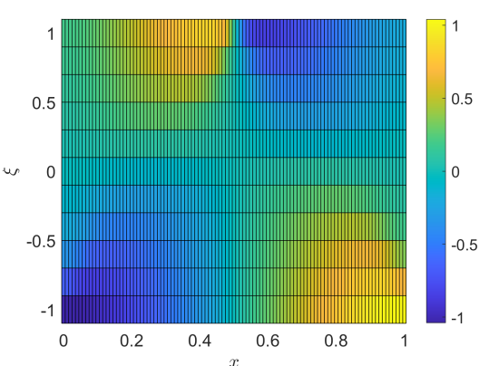
Figure 1: Numerical solutions obtained by the stochastic collocation LxF method (left) and the proposed method (right). Initial data are $u(0,x,\xi)=\xi\sin(2\pi x).$ The final time $T=1/4.$

In the presented method the entropy has been minimized to obtain an approximation to the Young measure. This is necessary to obtain the entropy solution as the following example illustrates. If, for example, we change the minimization problem to feasibility only, i.e., we set $\eta(\mathbf{u})=1$ in the cost functional of problem (2.26), the result in Figure 2 is obtained. Comparing with Figure 1 we observe that in this case the scheme selects the wrong weak solution consisting of rarefaction waves even in the case $\xi>0.$ This is not the correct weak entropy solution.

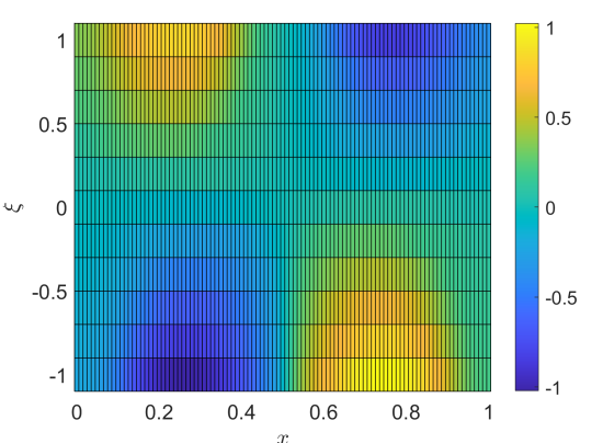
Figure 2: Numerical solution obtained by the proposed method with modified cost functional in the linear program (2.26). Initial data are $u(0,x,\xi)=\xi\sin(2\pi x).$ The final time is $T=1/4.$

3.3 Riemann Problem for the Isentropic Euler System

The proposed method is applicable also for systems of hyperbolic conservation laws. We consider random isentropic Euler system. We take equidistant grid in $(x,\xi)\in[-1,1]\times[-1,1]$ with $N_{x}=100$ and $N_{\xi}=10$ points.

The phase domain for $u=(\rho,q)^{T}$ is chosen to be $[0.05,2.5]\times[-1.0,1.5]$ and discretized using $N_{u}=25$ points in each direction. Terminal time is $T=1/4.$ The initial data for $(\rho,q)(0,\cdot,\cdot)$ are chosen to have 1-shocks and a 1-rarefaction waves depending on the value of $\xi.$ To this end, we state the $1-$forward Lax-curve starting at non–vacuum datum $U_{L}=(\rho_{L},q_{L}).$

$$U(s;U_{L}):= \left(s,s\;\rho_{L}-\sqrt{\frac{s}{\rho_{L}}(s-\rho_{L})(p(s)-p(\rho_{L}))}\right),\mbox{ if }\^{A}\nobreakspace s\geq\rho_{L},$$ (3.9a)

$$U(s;U_{L}):= \left(s,s\;\rho_{L}-s\left(\log(s)-\log(\rho_{L})\right)\right),\mbox{ if }\^{A}\nobreakspace 0<s<\rho_{L}.$$ (3.9b)

Using formula (3.9) the following Riemann problem is considered. The left initial datum is deterministic $U_{L}=(1,1)^{T}$, and the right datum depends on the value of $\xi$.

$$u_{0}(x,\xi):= U_{L},\;\mbox{ for }x<0\mbox{ and all }\xi,$$ (3.10)

$$u_{0}(x,\xi):= U(\frac{1}{2}\xi+U_{L};U_{L}),\mbox{ for }x>0\mbox{ and all }\xi,$$ (3.11)

The solution exhibits a shock wave for $\xi<0$ in the first family and a rarefaction wave of the first family for all values of $\xi\geq 0.$ In Figure 3 simulation results on the given spatial and random grids for both the proposed method as well as the reference stochastic collocation Lax-Friedrichs finite volume method (3.5) are given. The time step $\Delta t$ is chosen according to the CFL condition (3.3) and computed at each discrete point in time $n\Delta t.$ The $L^{1}-$error (3.7) in the density $\rho$ at time $T=1/4$ is $err=4.3707e-04$ and in the momentum $q$ it is $err=2.5379e-04.$ The solution structure for different values of $\xi$ is also correctly identified with the proposed method.

    

    

    

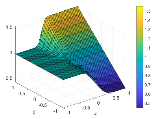
Figure 3: Simulation results using a proposed method for the Euler system with the initial data given by (3.10). The solution $u(t,\cdot,\cdot)$ is shown at time $T=1/4.$ In the top part the initial data are shown. The second row presents the results of the stochastic collocation LxF method and the bottom part shows the results obtained by the proposed methods. To the left the density is shown and to the right the momentum is presented.

4 Discussion and Outlook

We have proposed a novel numerical method for random hyperbolic conservation laws based on the concept of measure-valued solutions. The method was presented for one-dimensional hyperbolic system and for one-dimensional random data. Generalization to multi-dimensional random space and multi-dimensional hyperbolic systems is straightforward. In the context of the linear programs this would however lead to possibly very high dimensional problems. Generalization to high–order numerical methods is possible as well. The high–order reconstruction will enter in the moments that in turn are used in the constraints of the linear program. Any high–order numerical flux can than be computed using the solution to the linear program.

Furthermore, in this work only numerical results for the basis functions $\phi_{i}(\xi)=\delta(\xi-\xi_{i})$, cf. (2.23) for its discrete representation, have been shown. However, our approach is more general and can use any orthonormal basis in random space. Hence, the suggested method yields a unifying framework for the treatment of random hyperbolic conservation laws. In particular, the proposed method is less intrusive than the stochastic Galerkin method using generalized polynomial chaos, since only the flux function needs to be replaced by the linear programming problem. The conservative variables and their high–order reconstruction, does not require any modification. Of course, it is still more intrusive than the Monte Carlo or stochastic collocation methods. The numerical results show that in the considered case of basis function the numerical solutions obtained by the new method and the standard stochastic collocation method are comparable. The proposed method is computationally less efficient due to the subsequent solutions of possibly large linear programs. We point out that our technique uses the underlying measure-valued representation of a solution and approximates the corresponding Young measure directly. As far as we know this is for the first time when such a direct computation of the measure-valued solutions is used in the framework of random problems.

Acknowledgments

The authors thank the Deutsche Forschungsgemeinschaft (DFG, German Research Foundation) for the financial support through 320021702/GRK2326, 333849990/GRK2379, SPP 2410 Hyperbolic Balance Laws in Fluid Mechanics: Complexity, Scales, Randomness (CoScaRa) within the Projects HE5386/26-1 (Numerische Verfahren für gekoppelte Mehrskalenprobleme,525842915), HE5386/27-1, LU1470/10-1 (Zufällige kompressible Euler Gleichungen: Numerik und ihre Analysis, 525853336) and LU1470/9-1 (An Active Flux method for the Euler equations, 525800857). M.H. has also received funding from the European Union’s Horizon Europe research and innovation programme under the Marie Sklodowska-Curie Doctoral Network Datahyking (Grant No.101072546) and HE5386/30-1 Effiziente Ermittlung von Temperaturfeldern mithilfe von Physics-Informed Neural Networks zur Modellierung des thermo-elastischen Verhaltens von Werkzeugmaschinen (537928890).
The work of M.L.-M. was also partially supported by the Gutenberg Research College and by the Deutsche Forschungsgemeinschaft - project number 233630050 - TRR 146. M.L.-M. is grateful to the Mainz Institute of Multiscale Modelling for supporting her research.

References

- [1] R. Abgrall and S. Mishra, Uncertainty quantification for hyperbolic systems of conservation laws, in Handbook of numerical methods for hyperbolic problems, vol. 18 of Handb. Numer. Anal., Elsevier/North-Holland, Amsterdam, 2017, pp. 507–544.
- [2] T. Barth, Non-intrusive uncertainty propagation with error bounds for conservation laws containing discontinuities, in Uncertainty quantification in computational fluid dynamics, vol. 92 of Lect. Notes Comput. Sci. Eng., Springer, Heidelberg, 2013, pp. 1–57.
- [3] J. P. Boyd, Chebyshev and Fourier spectral methods, Dover Publications, Inc., Mineola, NY, second ed., 2001.
- [4] A. Bressan, Hyperbolic systems of conservation laws, vol. 20 of Oxford Lecture Series in Mathematics and its Applications, Oxford University Press, Oxford, 2000. The one-dimensional Cauchy problem.
- [5] C. Cardoen, S. Marx, A. Nouy, and N. Seguin, A moment approach for entropy solutions of parameter-dependent hyperbolic conservation laws, Numer. Math., 156 (2024), pp. 1289–1324.
- [6] A. Chertock, M. Herty, A. S. Iskhakov, S. Janajra, A. Kurganov, and M. Lukáčová-Medviďová, New high-order numerical methods for hyperbolic systems of nonlinear PDEs with uncertainties, Commun. Appl. Math. Comput., 6 (2024), pp. 2011–2044.
- [7] A. Chertock, M. Herty, A. Kurganov, and M. Lukáčová-Medviďová, Challenges in stochastic galerkin methods for nonlinear hyperbolic systems with uncertainty, to appear: Springer Volume on Advances in Nonlinear Hyperbolic Partial Differential Equations, (2024).
- [8] C. M. Dafermos, Hyperbolic conservation laws in continuum physics, vol. 325 of Grundlehren der mathematischen Wissenschaften [Fundamental Principles of Mathematical Sciences], Springer-Verlag, Berlin, fourth ed., 2016.
- [9] D. Dai, Y. Epshteyn, and A. Narayan, Hyperbolicity-preserving and well-balanced stochastic Galerkin method for shallow water equations, SIAM J. Sci. Comput., 43 (2021), pp. A929–A952.
- [10] B. Després, G. Poëtte, and D. Lucor, Robust uncertainty propagation in systems of conservation laws with the entropy closure method, in Uncertainty quantification in computational fluid dynamics, vol. 92 of Lect. Notes Comput. Sci. Eng., Springer, Heidelberg, 2013, pp. 105–149.
- [11] H. C. Elman, C. W. Miller, E. T. Phipps, and R. S. Tuminaro, Assessment of collocation and Galerkin approaches to linear diffusion equations with random data, Int. J. Uncertain. Quantif., 1 (2011), pp. 19–33.
- [12] O. G. Ernst, A. Mugler, H.-J. Starkloff, and E. Ullmann, On the convergence of generalized polynomial chaos expansions, ESAIM Math. Model. Numer. Anal., 46 (2012), pp. 317–339.
- [13] L. C. Evans and R. F. Gariepy, Measure theory and fine properties of functions, Textbooks in Mathematics, CRC Press, Boca Raton, FL, revised ed., 2015.
- [14] H. Federer, Geometric measure theory, vol. Band 153 of Die Grundlehren der mathematischen Wissenschaften, Springer-Verlag New York, Inc., New York, 1969.
- [15] E. Feireisl and M. Lukáčová-Medviďová, Convergence of a stochastic collocation finite volume method for the compressible Navier-Stokes system, Ann. Appl. Probab., 33 (2023), pp. 4936–4963.
- [16] E. Feireisl, M. Lukáčová-Medviďová, and H. Mizerová, Convergence of finite volume schemes for the Euler equations via dissipative measure-valued solutions, Found. Comput. Math., 20 (2020), pp. 923–966.
- [17] E. Feireisl, M. Lukáčová-Medviďová, H. Mizerova, and B. She, Numerical analysis of compressible fluid flows, vol. 20 of MS&A. Modeling, Simulation and Applications, Springer, Cham, 2021.
- [18] A. Gelb and E. Tadmor, Enhanced spectral viscosity approximations for conservation laws, in Proceedings of the Fourth International Conference on Spectral and High Order Methods (ICOSAHOM 1998) (Herzliya), vol. 33, 2000, pp. 3–21.
- [19] S. Gerster and M. Herty, Entropies and symmetrization of hyperbolic stochastic Galerkin formulations, Commun. Comput. Phys., 27 (2020), pp. 639–671.
- [20] S. Gerster, M. Herty, and A. Sikstel, Hyperbolic stochastic Galerkin formulation for the -system, J. Comput. Phys., 395 (2019), pp. 186–204.
- [21] M. Herty, A. Kolb, and S. Müller, Multiresolution analysis for stochastic hyperbolic conservation laws, IMA J. Numer. Anal., 44 (2024), pp. 536–575.
- [22] J. S. Hesthaven, S. Gottlieb, and D. Gottlieb, Spectral methods for time-dependent problems, vol. 21 of Cambridge Monographs on Applied and Computational Mathematics, Cambridge University Press, Cambridge, 2007.
- [23] A. Kurganov and Y. Liu, New adaptive artificial viscosity method for hyperbolic systems of conservation laws, J. Comput. Phys., 231 (2012), pp. 8114–8132.
- [24] J. Kusch and M. Frank, Intrusive methods in uncertainty quantification and their connection to kinetic theory, Int. J. Adv. Eng. Sci. Appl. Math., 10 (2018), pp. 54–69.
- [25] J. Kusch, R. G. McClarren, and M. Frank, Filtered stochastic Galerkin methods for hyperbolic equations, J. Comput. Phys., 403 (2020). Paper No. 109073, 19 pp.
- [26] S. Mehrotra, On the implementation of a primal-dual interior point method, SIAM J. Optim., 2 (1992), pp. 575–601.
- [27] S. Mishra and C. Schwab, Monte-Carlo finite-volume methods in uncertainty quantification for hyperbolic conservation laws, in Uncertainty quantification for hyperbolic and kinetic equations, vol. 14 of SEMA SIMAI Springer Ser., Springer, Cham, 2017, pp. 231–277.
- [28] S. Mishra, C. Schwab, and J. ˇSukys, Multi-level Monte Carlo finite volume methods for uncertainty quantification of acoustic wave propagation in random heterogeneous layered medium, J. Comput. Phys., 312 (2016), pp. 192–217.
- [29] M. P. Pettersson, G. Iaccarino, and J. Nordström, Polynomial chaos methods for hyperbolic partial differential equations, Mathematical Engineering, Springer, Cham, 2015. Numerical techniques for fluid dynamics problems in the presence of uncertainties.
- [30] P. Pettersson, G. Iaccarino, and J. Nordström, A stochastic Galerkin method for the Euler equations with Roe variable transformation, J. Comput. Phys., 257 (2014), pp. 481–500.
- [31] G. Poëtte, B. Després, and D. Lucor, Uncertainty quantification for systems of conservation laws, J. Comput. Phys., 228 (2009), pp. 2443–2467.
- [32] L. Schlachter and F. Schneider, A hyperbolicity-preserving stochastic Galerkin approximation for uncertain hyperbolic systems of equations, J. Comput. Phys., 375 (2018), pp. 80–98.
- [33] G. Szego, Orthogonal polynomials, vol. Vol. XXIII of American Mathematical Society Colloquium Publications, American Mathematical Society, Providence, RI, fourth ed., 1975.
- [34] E. Tadmor, Convergence of spectral methods for nonlinear conservation laws, SIAM J. Numer. Anal., 26 (1989), pp. 30–44.
- [35] J. Tryoen, O. Le Maître, M. Ndjinga, and A. Ern, Intrusive Galerkin methods with upwinding for uncertain nonlinear hyperbolic systems, J. Comput. Phys., 229 (2010), pp. 6485–6511.
- [36] N. Wiener, The Homogeneous Chaos, Amer. J. Math., 60 (1938), pp. 897–936.
- [37] D. Xiu, Numerical methods for stochastic computations, Princeton University Press, Princeton, NJ, 2010. A spectral method approach.
- [38] D. Xiu and J. S. Hesthaven, High-order collocation methods for differential equations with random inputs, SIAM J. Sci. Comput., 27 (2005), pp. 1118–1139.
- [39] Y. Zhang, Solving large-scale linear programs by interior-point methods under the MATLAB environment, Optim. Methods Softw., 10 (1998), pp. 1–31.