A recursive Bayesian neural network for constitutive modeling of sands under monotonic loading

Abstract

In geotechnical engineering, constitutive models play a crucial role in describing soil behavior under varying loading conditions. Data-driven deep learning (DL) models offer a promising alternative for developing predictive constitutive models. When prediction is the primary focus, quantifying the predictive uncertainty of a trained DL model and communicating this uncertainty to end users is crucial for informed decision-making.

This study proposes a recursive Bayesian neural network (rBNN) framework, which builds upon recursive feedforward neural networks (rFFNNs) by introducing generalized Bayesian inference for uncertainty quantification. A significant contribution of this work is the incorporation of a sliding window approach in rFFNNs, allowing the models to effectively capture temporal dependencies across load steps. The rBNN extends this framework by treating model parameters as random variables, with their posterior distributions inferred using generalized variational inference.

The proposed framework is validated on two datasets: (i) a numerically simulated consolidated drained (CD) triaxial dataset employing a hardening soil model and (ii) an experimental dataset comprising 28 CD triaxial tests on Baskarp sand. Comparative analyses with LSTM, Bi-LSTM, and GRU models demonstrate that the deterministic rFFNN achieves superior predictive accuracy, attributed to its transparent structure and sliding window design. While the rBNN marginally trails in accuracy for the experimental case, it provides robust confidence intervals, addressing data sparsity and measurement noise in experimental conditions. The study underscores the trade-offs between deterministic and probabilistic approaches and the potential of rBNNs for uncertainty-aware constitutive modeling.

Keywords Sand Constitutive Modeling  $\cdot$ Deep Learning  $\cdot$ Recursive Neural Network  $\cdot$ Bayesian Modeling  $\cdot$ Generalized Variational Inference

1 Introduction

Constitutive modeling of soil is a key challenge in geotechnical engineering due to its complex, heterogeneous, and anisotropic properties. Unlike metals, soils consist of discrete particles, and their behavior is influenced by environmental conditions such as moisture and stress history, resulting in nonlinear and path-dependent behavior [1]. Despite these challenges, accurate constitutive models for soil are crucial for predicting soil behavior under various loading conditions. Accurate models are crucial for applications such as landslide prediction [2], helping to anticipate and mitigate slope failures [3], designing excavations and tunneling [4], and foundation engineering [5], ensuring the stability and longevity of structures by predicting soil responses to imposed loads.

Traditional models, such as those based on elasticity and plasticity, offer foundational approaches but often struggle to capture soil’s post-yield complexities. Simple elastic models, like those based on Hooke’s law [6], fail to account for strain hardening, softening, and other nuanced behaviors that emerge beyond the yield point. More advanced constitutive models, such as viscoelastic [7, 8], hyperelastic [9], and elastoplastic [10, 11, 12, 13] formulations, aim to capture a broader range of soil behaviors, but they become increasingly complex and harder to interpret as they account for factors like creep, dilatancy, and non-linear stress-strain relationships.

When focusing specifically on sands, the challenges in modeling become more pronounced due to behaviors such as dilatancy [14], state dependence [15], and anisotropy [16], which play a significant role in their mechanical response. While clays also exhibit these behaviors, they tend to manifest differently and are generally less pronounced compared to sands. The discrete, angular nature of sand particles and their interactions under stress make it difficult for traditional models to accurately predict their behavior. A large number of phenomenological models and a few mechanistic models have been developed to better capture the specific behaviors observed in sands. These models vary in complexity and applicability, including linear elastic models [6], linear elastic perfectly plastic models (Mohr-Coulomb [17], non-linear models (hardening soil [18], non-linear Mohr-Coulumb [19], critical state-based models (Nor-Sand [20], Severn-Trent [21], UH [10], SANISAND [22], SIMSAND [23], ANICREEP [24], hypoplastic [25]), and micromechanical models [26].

While these models aim to capture the intricate mechanics of sands, their increasing complexity can limit practical application due to the numerous parameters requiring calibration [27, 28]. Further, the increased complexity of advanced constitutive models in numerical simulations often heightens the risk of non-convergence. As a result, deep learning (DL) techniques have emerged as a promising alternative. DL models, by leveraging extensive experimental datasets, can learn complex stress-strain relationships without relying on detailed mechanistic formulations. This makes them more efficient for predictive modeling of sand behavior, and has contributed to their growing popularity in constitutive modeling for a wide range of geomaterials, including sand [29].

Early efforts to apply DL to the constitutive modeling of sand primarily used feedforward neural networks (FFNNs) to predict stress-strain behavior under monotonic loading conditions, both drained and undrained [30, 31, 32, 33, 34]. These models were trained on numerous examples of stress-strain data at different quasi-static loading steps, where stress was predicted based on strain and strain increments (see Fig.˜1(a)). However, a major limitation of these FFNNs was the accumulation of prediction errors over the entire loading history, during testing, especially when relying solely on initial stress values to predict future states.

To address this issue, feedback neural networks, here referred to as recursive FFNNs (rFFNNs), were introduced [35, 36]. Recursive FFNNs incorporate previous predictions into subsequent inputs, allowing the model to better handle the sequential nature of stress-strain relationships across multiple loading steps in comparison to static FFNN fits (see Fig.˜1(b)). However, training rFFNNs, as described in literature [35, 36], involves predicting the entire series from the initial stress value all at once. This approach is suboptimal because measurement errors can accumulate over time, potentially leading to less accurate predictions and poor generalization accuracy. In the current study, we introduce the concept of training the rFFNNs over multiple overlapping sliding windows with varying starting points. The recursive use of predictions within these sliding windows, where the window length itself becomes a hyperparameter, improves training efficiency leading to better prediction accuracy.

(a) FFNN

(b) Recursive-FFNN

Figure 1: Comparison of FFNN and rFFNN training approach: (a) A single-step FFNN utilizes the measured current stress state and strain increment to predict the subsequent stress state. (b) The rFFNN incorporates the predicted stress state from the current step as feedback to predict the next stress state, recursively incorporating prior predictions as inputs to capture sequential and path-dependent stress-strain behavior.

Recently, more sophisticated architectures, such as recurrent neural networks (RNNs), Long Short-Term Memory (LSTM), and Gated Recurrent Units (GRUs) have been used. The RNNs emerged as a natural progression in sand constitutive modeling due to their ability to maintain a memory of previous inputs, which informs the current prediction through the “hidden state.” Unlike first-order Markov models that rely solely on the present state, RNNs have the capacity to capture temporal dependencies over multiple load steps by summarizing previous information through hidden states. However, early RNNs encountered challenges such as exploding and vanishing gradients, limiting their effectiveness in capturing stress-strain-volume change behavior of granular materials [37, 38, 39]. To address these limitations, advanced architectures like LSTM [40] and its variants like GRU [41] were introduced. These models incorporate gating mechanisms that regulate information flow, enabling them to retain relevant information over longer sequences while mitigating gradient-related issues. As a result, these advanced RNN variants have proven effective in accurately representing complex patterns in sand constitutive behavior [29, 42, 43, 44, 45].

While ML and DL models offer attractive alternatives in capturing complex relationships without the need for explicit physical laws, they also present challenges, such as optimizing training techniques, managing limited and noisy data, effectively quantifying uncertainties, and minimizing overfitting risks. These models are generally trained on either simulated or experimental data; simulated data is based on a limited number of simulations, while experimental data tends to be both sparse and noisy. As such, data-driven models must inherently account for the “limited-data uncertainty” for simulated data. For experimental data, uncertainty arises additionally due to modeling and the presence of measurement variability (noisy data uncertainty) in data. Traditional deterministic DL models, including FFNNs, rFFNNs, RNNs, and LSTMs, only yield point estimates, failing to quantify the uncertainties inherent in the data. However, implementing uncertainty quantification (UQ) in ML/DL models is also crucial since it provides end-users with confidence bounds that reflect prediction quality and support better-informed decision-making in geotechnical applications.

In this study, the FFNNs are made uncertainty-aware by treating the model parameters $\bm{{\beta}}$ as random variables and introducing a deterministic uncertainty layer as the last layer in the FFNN. By deterministic uncertainty layer, we mean that the output is a distribution (in our case Gaussian), with the mean and standard deviation as a deterministic function of the FFNN parameters. This uncertainty output layer allows us to write a Gaussian distribution over the predictions with an inferred mean and standard deviation. As such, the model parameters $\bm{{\beta}}$ becomes amenable to Bayesian inference, akin to Bayesian neural networks (BNNs)[46, 47, 48]. These random variables, characterized by probability distributions, capture the uncertainty in the parameters. However, as will be explained later in Section˜3.2, a recursive loss-based formulation over multiple overlapping sliding windows causes a departure from likelihood-based formulation. Therefore, we adopt a generalized Bayesian inference framework, which allows the use of loss function instead of likelihood function ([49, 50, 51]). Additionally, Bayesian approaches mitigate overfitting by automatically regularising the models by using a prior distribution as inductive bias. There exists a work in soil constitutive modeling, where Bayesian NNs have been applied for the purpose of regularization [52]. Similarly, methods like Monte Carlo (MC) dropout [53], have been used for regularization but can also be used for UQ [54]. However, MC dropout does not provide the comprehensive probabilistic modeling that a fully Bayesian approach offers [53]. A Bayesian paradigm, offers a systematic way of UQ, while also preventing overfitting since they are automatically regularized.

To the best of the authors’ knowledge, this study presents the first fully Bayesian framework for constitutive modeling of sands by implementing a recursive generalized Bayesian neural network (rBNN) under monotonic loading. The novelty of the work is twofold: (a) improvement of training and generalization of rFFNNs by using the sliding windows approach, (b) making the rFFNNs uncertainty-aware, by introducing a deterministic uncertainty output layer and employing Bayesian modeling to infer probability distributions over the neural network’s parameters, using the generalized variational inference framework. This approach not only prevents overfitting but also provides predictive uncertainty estimates.

The paper is organized as follows: the problem statement is described in Section˜2, followed by the methodology Section˜3, which outlines the rFFNN and development of Bayesian extension of rFFNN, termed as rBNN. Section˜4 focuses on performance assessment, presenting results for both simulated and experimental datasets, while highlighting the model’s accuracy and uncertainty quantification capabilities. The paper concludes with a discussion section (Section˜5) that highlights the key findings, significance, and potential future directions, followed by a separate conclusion section to summarize the work comprehensively.

2 Problem Setup

This study aims to develop an uncertainty-aware probabilistic constitutive model for sandy soils, using data from $M$ strain-controlled quasi-static consolidated drained (CD) triaxial tests. Each test records the stress-strain-volume change responses of a sand sample under controlled loading conditions. Initially, the sand sample is consolidated under a constant confining pressure $\sigma_{3}$, and then incremental compressive axial strains $\text{d}\epsilon$ are applied through quasi-static loading, illustrated in Fig.˜2. At each load step, the mean effective stress $(p)$ and deviatoric stress ($q$) are computed as:

$$p=\frac{\sigma_{1}+2\sigma_{3}}{3},\quad q=\sigma_{1}-\sigma_{3}$$ (1)

while the void ratio $e$ is derived based on the initial void ratio $e_{0}$ and the measured volume change, modified due to the rearrangement of particles. These load steps represent pseudo-time indices, allowing the modeling of sequential soil responses.

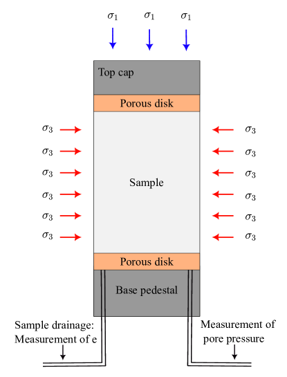
Figure 2: Schematic of the Consolidated drained (CD) triaxial test setup.

Each triaxial test $m\in\{1,2,\dots,M\}$ consists of multiple load steps $t\in\{1,\dots,N\}$, with a state vector at each step defined as:

$$\bm{{s}}^{(m)}_{t}=\begin{bmatrix}p^{(m)}_{t},\;q^{(m)}_{t},\;e^{(m)}_{t}\end{bmatrix}^{T}$$ (2)

This state vector characterizes the mechanical behavior of the soil for the $m^{\text{th}}$ triaxial test at the $t^{\text{th}}$ load step. The dataset is augmented with triaxial test constants $\bm{{\theta}}^{(m)}=\left\{\sigma_{3}^{(m)},e_{0}^{(m)}\right\}$, which vary across tests but remain constant within a single test, and the axial strain $\epsilon^{(m)}$ and its increment $d\epsilon^{(m)}$, which together is referred to as the exogenous inputs and denoted by $\bm{{u}}^{(m)}=\left\{\epsilon^{(m)},d\epsilon^{(m)}\right\}$. This systematic variation of $\bm{{\theta}}^{(m)}$ enables the representation of diverse mechanical behaviors of sand samples with the same constitutive properties.

The multiple triaxial tests dataset is represented as follows:

$$\text{Dataset}=\begin{Bmatrix}\bm{{\theta}}^{(m)},\begin{pmatrix}p^{(m)}_{0}\\ q^{(m)}_{0}\\ e^{(m)}_{0}\\ \epsilon^{(m)}_{0}\\ \text{d}\epsilon^{(m)}_{0}\end{pmatrix},\ldots,\begin{pmatrix}p^{(m)}_{t}\\ q^{(m)}_{t}\\ e^{(m)}_{t}\\ \epsilon^{(m)}_{t}\\ \text{d}\epsilon^{(m)}_{t}\end{pmatrix},\ldots,\begin{pmatrix}p^{(m)}_{N}\\ q^{(m)}_{N}\\ e^{(m)}_{N}\\ \epsilon^{(m)}_{N}\end{pmatrix}\end{Bmatrix}_{m=1}^{M}$$

The goal is to characterize the evolution of soil states through the mapping $f_{\beta}$, where a deterministic framework relates the previous state to the next:

$$\bm{{s}}_{t}^{(m)}=f_{\bm{{\beta}}}\left(\bm{{s}}_{t-1}^{(m)},\bm{{u}}_{t}^{(m)},\bm{{\theta}}^{(m)}\right),\quad t=1,\ldots,N,\;\;m=1,\ldots,M$$ (3)

However, deterministic models do not inherently quantify uncertainty, which is critical for understanding the variability in soil responses and ensuring confidence in predictions. In contrast, probabilistic models explicitly quantify uncertainty, enabling richer representations of confidence in predictions.

To address this, a probabilistic mapping $f_{\beta}$ that relates the previous state to the current state, conditioned on exogenous inputs and triaxial test constants, is proposed. Specifically, given $M$ datasets, each structured as:

$$\mathcal{S}^{(m)}=\left\{\bm{{u}}^{(m)}_{1:{N}},\bm{{s}}^{(m)}_{1:{N}},\bm{{\theta}}^{(m)}\right\},\quad m=1,\ldots,M$$ (4)

the objective is to characterize the predictive probability distribution over the states $\bm{{s}}$, conditioned on the inputs $\bm{{u}}$ and the test constants $\bm{{\theta}}$, expressed as:

$$p\left(\bm{{s}}\mid\bm{{u}},\bm{{\theta}}\right)$$

which encodes both the predictions and the associated uncertainties.

To facilitate efficient inference, the conditional distribution is modeled as a Gaussian distribution. The modeling choice simplifies the task by reducing it to the estimation of two key parameters: the mean and covariance of the Gaussian distribution. The proposed framework uses a generalized variational Bayesian inference integrated with a windowed recursive FFNN structure, to fit the probabilistic representation, quantifying uncertainty across load steps.

3 Methodology

The proposed framework combines the strengths of deterministic recursive FFNN models with the uncertainty quantification capabilities of Bayesian neural networks. By introducing a windowed recursive structure and employing a pseudo-likelihood formulation for overlapping data subsets, the framework addresses challenges specific to sequential modeling in triaxial test datasets. Additionally, the use of variational inference enables scalable posterior estimation, ensuring computational feasibility for high-dimensional parameter spaces.

In what follows next, we provide an introduction to recursive feedforward neural networks (rFFNNs) and the proposed sliding window approach that enables recursive predictions within overlapping subsets of data. Subsequently, a Bayesian extension to rFFNNs, termed recursive Bayesian FFNNs (rBNNs), is presented, highlighting its probabilistic formulation and capability to quantify uncertainties. The discussion concludes with the formulation of a generalized likelihood and the approximation of the posterior distribution via generalized variational inference, which is crucial for uncertainty quantification and propagation in data-driven probabilistic constitutive modeling of sand. A subsection mentioning the data normalization for improved modelling is presented at the very end of this section.

3.1 Recursive Feedforward Neural Networks (rFFNNs)

rFFNNs extend the capabilities of conventional FFNNs by incorporating recursive feedback to refine predictions over an extended forecasting horizon, as illustrated in Fig.˜1(b). While FFNNs rely on direct mappings from the current state to the next state, they do not account for the compounding errors that arise during multi-step recursive predictions. In contrast, rFFNNs use their own predictions as inputs for subsequent steps, allowing the model to iteratively adjust and improve its forecast. This feedback loop enhances the rFFNN’s ability to capture complex temporal dependencies and reduce prediction error accumulation across multiple steps. Consequently, rFFNNs are particularly well-suited for multi-step forecasting tasks, where temporal relationships play a significant role.

3.1.1 Sliding window approach for training rFFNNs

To enable the model to effectively learn temporal dependencies, the loading series data is segmented into overlapping subsets, or sliding windows, of a fixed length $H$. Each window contains sequences of states, exogenous inputs, and triaxial test constants, as described below:

$$\mathcal{S}_{H,k}^{(m)}=\left\{\bm{{s}}_{t-1}^{(m)},\bm{{u}}_{t}^{(m)},\bm{{\theta}}^{(m)}\right\}_{t={k}}^{k+H-1},\quad k=1,\dots,N-H+1,\;m=1,\ldots,M$$ (5)

Here, $\mathcal{S}_{H,k}^{(m)}$ is a window from the $m^{\text{th}}$ triaxial test, comprising triaxial test constants $\bm{{\theta}}$ and a certain $H$-long sequence of state variables $\bm{{s}}$ and exogenous inputs $\bm{{u}}$. For a dataset with $N$ load steps, a total of $(N-H+1)$ windows are generated, as depicted in Fig.˜3. Training over these sliding windows enables the rFFNN to focus on localized temporal patterns, which is crucial for learning sequential dependencies effectively.

When the window length $H=1$, the sliding window approach reduces the rFFNN to a standard FFNN, as the prediction is limited to a single step without recursion. Conversely, when $H=N$, the method becomes equivalent to a traditional rFFNN [31], where the entire loading series is predicted recursively using a single window. This flexibility allows the framework to balance the trade-off between capturing short-term patterns and long-term dependencies.

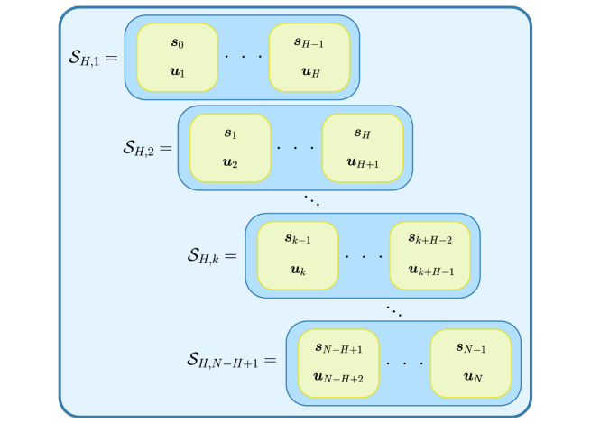
Figure 3: Illustration of the sliding window approach for training data preparation. Each window $\mathcal{S}_{H,k}$ captures a fixed-length sequence of state variables $\bm{{s}}$ and inputs $\bm{{u}}$ over $H$ load steps, enabling the model to learn dependencies. Windows overlap, spanning $N-H+1$ segments, with triaxial test constants $\bm{{\theta}}$.

3.1.2 Recursive prediction within windowed subsets

For each window $\mathcal{S}_{H,k}^{(m)}$, the rFFNN performs recursive predictions starting with the initial measured state $\bm{{s}}_{k-1}^{(m)}$ to predict the next state $\hat{\bm{{s}}}_{k}^{(m)}$, given the input $\bm{{u}}_{k}^{(m)}$ and triaxial test constant $\bm{{\theta}}^{(m)}$. The predicted states are recursively fed back into the rFFNN, alongside the inputs from the subsequent load step, to predict the future states within the window. This recursive mechanism, illustrated in Fig.˜4, can be expressed mathematically as:

$$\begin{split}\hat{\bm{{s}}}_{k}^{(m)}&=f_{\bm{{\beta}}}\left(\bm{{s}}_{k-1}^{(m)},\bm{{u}}_{k}^{(m)},\bm{{\theta}}^{(m)}\right)\\ \hat{\bm{{s}}}_{k+1}^{(m)}&=f_{\bm{{\beta}}}\left(\hat{\bm{{s}}}_{k}^{(m)},\bm{{u}}_{k+1}^{(m)},\bm{{\theta}}^{(m)}\right)\\ &\vdots\\ \hat{\bm{{s}}}_{k+H-1}^{(m)}&=f_{\bm{{\beta}}}\left(\hat{\bm{{s}}}_{k+H-2}^{(m)},\bm{{u}}_{k+H-1}^{(m)},\bm{{\theta}}^{(m)}\right)\end{split}$$ (6)

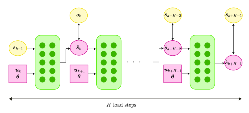
Figure 4: Recursive state prediction over a $H$-length sliding window using a deterministic rFFNN for the data subset $\mathcal{S}_{H,k}$.

3.1.3 Loss computation for training rFFNNs

The loss $L_{H,k}^{(m)}$ for a windowed subset $\mathcal{S}^{(m)}_{H,k}$ is computed as the average discrepancy between the predicted states $\hat{\bm{{s}}}^{(m)}_{t}$ and the corresponding observed states $\bm{{s}}_{t}^{(m)}$ across all load steps within the window, calculated as below:

$$L_{H,k}^{(m)}=\frac{1}{H}\sum_{t=k}^{k+H-1}\ell\left(\bm{{s}}_{t}^{(m)},\hat{\bm{{s}}}_{t}^{(m)}\right)$$ (7)

The function $\ell$ is a user-chosen loss metric, such as the squared loss, absolute loss, and Huber loss, depending on the requirements of the application.

The average loss $L$ across all loading series of states $\left\{\bm{{s}}^{(m)}_{0:N}\right\}_{m=1}^{M}$, comprising $M$ triaxial tests with $N$ load steps each, is determined by summing the loss over all windowed subsets, given the complete loading series of control inputs $\left\{\bm{{u}}^{(m)}_{1:N},\bm{{\theta}}^{(m)}\right\}_{m=1}^{M}$:

$$L=\sum_{m=1}^{M}\frac{1}{M(N-H+1)}\sum_{k=1}^{(N-H+1)}L_{H,k}^{(m)}$$ (8)

While rFFNN provides an effective framework for deterministic recursive predictions, it lacks the ability to quantify uncertainties, which is crucial in applications requiring high reliability, such as geotechnical design. To overcome this limitation, we extend the rFFNN framework into a Bayesian paradigm, to provide both predictions and associated uncertainties. This transition allows the model to better account for uncertainties.

3.2 Generalized Bayesian rFFNNs (rBNNs)

Building upon the deterministic foundation of rFFNN, the next step involves integrating uncertainty quantification through Bayesian methods. The rBNN framework extends rFFNN by treating model parameters as random variables, allowing for probabilistic predictions and a richer representation of model uncertainty. This approach aligns closely with Bayesian neural networks (BNNs) [47, 53], which enables the estimation of both epistemic uncertainty (arising from limited training data) and aleatoric uncertainty (due to inherent noise in data). The key enhancement of rBNNs over rFFNNs is as follows:

1. Random variable modeling: The parameters of the rBNN, represented as the vector $\bm{{\beta}}$, are treated as a vector-valued random variable, characterized by a joint probability distribution. This allows the model to capture epistemic uncertainty.

2. Deterministic output uncertainty layer: A deterministic layer at the output of the rBNN predicts the mean and covariance of a Gaussian distribution for the next state, capturing aleatoric uncertainty due to noise in the training data.

3. Use of pseudo-likelihood: Unlike traditional Bayesian methods, where the likelihood is derived from a probabilistic model of the data, we employ a pseudo-likelihood derived from the recursive predictions over several overlapping subsets of data.

Illustration of the rBNN can be found in Fig.˜5. In this formulation, the neural network parameters $\bm{{\beta}}$ are not directly learned, instead the posterior distribution over the parameter vector $\bm{{\beta}}$ is inferred within a generalized Bayesian framework.

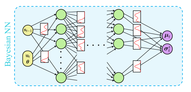
Figure 5: Depiction of rBNN where model parameters are treated as random variables, and the output layer predicts the mean and diagonal variances of a Gaussian distribution for the subsequent state.

However, the high-dimensional nature of parameter vector $\bm{{\beta}}$ poses difficulty for posterior inference. Analytical solutions are intractable, and Markov chain Monte Carlo (MCMC) methods, while exact, are computationally prohibitive for this application. As a more efficient alternative, variational Bayesian inference is employed to approximate the posterior distribution using a simpler, tractable family of distributions.

In the following subsections, we outline the essential components of the generalized Bayesian rFFNN: the prior distribution, the pseudo-likelihood, the posterior approximation, and the posterior predictive distribution.

3.2.1 Prior distribution

The prior distribution represents the initial beliefs about the parameter vector $\bm{{\beta}}$ before observing any data. In the context of deep learning, especially for neural networks, a common choice for the prior is a fully factorized standard Gaussian distribution [55], that is, each component of the parameter vector $\beta_{l}$ is assumed to be independent and identically distributed, drawn from a Gaussian distribution $\mathcal{N}$ with zero mean and unit variance. This choice is motivated by its simplicity, computational efficiency, and mathematical convenience during inference. The prior can be expressed as:

$$p(\bm{{\beta}})=\prod_{l=1}^{L}p({\beta}_{l})=\prod_{l=1}^{L}\mathcal{N}\left({\beta}_{l};0,1\right)=\mathcal{N}\left(\bm{{\beta}};\bm{{0}},\mathbf{I}_{L}\right),$$ (9)

where $L$ denotes the dimensionality of the model parameter vector $\bm{{\beta}}$ and $\mathbf{I}_{L}$ represents the $L\times L$ identity matrix. This prior not only simplifies the posterior inference process but also serves as a regularizer, helping to mitigate overfitting when the training data is limited. By assigning higher probability to parameters close to zero, the Gaussian prior encourages simpler models and prevents the parameters from growing arbitrarily large, particularly in high-dimensional settings.

3.2.2 Pseudo-likelihood formulation

In classical Bayesian inference, the likelihood is derived from a probabilistic model that describes the data-generating process; typically this assumes independence or predefined dependencies among observations in the data. However, in the case of rFFNNs, the sliding window approach introduces overlapping sequences, leading to repeated use of the same observed data points across windows. This overlap makes the direct use of a conventional likelihood function difficult. To overcome this issue, we employ a pseudo-likelihood formulation, which functions similarly to a generic loss function and is particularly advantageous for datasets with overlapping windows. This formulation not only reduces computational complexity but also enables the integration of uncertainty quantification and error propagation into a generalized Bayesian framework [56].

For the $t^{\text{th}}$ load step in the $k^{\text{th}}$ window of the $m^{\text{th}}$ triaxial test, the conditional distribution of the state vector $\bm{{s}}_{t}^{(m)}$ is modeled as:

$$p\left(\bm{{s}}_{t}^{(m)}\mid\bm{{s}}_{t-1}^{(m)},\bm{{u}}_{t}^{(m)},\bm{{\theta}}^{(m)},\bm{{\beta}}\right)=\mathcal{N}\left(\bm{{s}}_{t}^{(m)};\bm{{\mu}}_{t}^{(m)},\bm{{\sigma}}_{t}^{2(m)}\right)$$ (10)

where the predicted mean vector $\bm{{\mu}}_{t}^{(m)}$ and the predicted diagonal variance vector $\bm{{\sigma}}_{t}^{2(m)}$ are the two outputs of the neural network $f_{\bm{{\beta}}}$:

$$\begin{split}\bm{{\mu}}_{t}^{(m)}(\bm{{\beta}})&=f_{\bm{{\beta}}}\left(\bm{{s}}_{t-1}^{(m)},\bm{{u}}_{t}^{(m)},\bm{{\theta}}^{(m)}\right)\\ \bm{{\sigma}}_{t}^{2(m)}(\bm{{\beta}})&=f_{\bm{{\beta}}}\left(\bm{{s}}_{t-1}^{(m)},\bm{{u}}_{t}^{(m)},\bm{{\theta}}^{(m)}\right)\end{split}$$ (11)

with $\bm{{\beta}}$ representing the neural network parameters (weights and biases).

We construct the likelihood for a $H$-length sliding window $\mathcal{S}_{H,k}^{(m)}$ by defining a joint distribution over the state sequence $\bm{{s}}_{k:k+H-1}^{(m)}=\left\{\bm{{s}}_{k}^{(m)},\ldots,\bm{{s}}_{k+H-1}^{(m)}\right\}$ for a given triaxial test $m$, with known initial state $\bm{{s}}_{k-1}^{(m)}$, as a product of conditional distributions:

$$\mathcal{L}_{H,k}^{(m)}(\bm{{\beta}})=p\left(\bm{{s}}_{k:k+H-1}^{(m)}\mid\bm{{u}}_{k:k+H-1}^{(m)},\bm{{\theta}}^{(m)},\bm{{\beta}}\right)=\prod_{t=k}^{k+H-1}p\left(\bm{{s}}_{t}^{(m)}\mid\bm{{s}}_{t-1}^{(m)},\bm{{u}}_{t}^{(m)},\bm{{\theta}}^{(m)},\bm{{\beta}}\right)$$ (12)

However, propagating the full joint distribution across the load steps is computationally prohibitive, especially for overlapping windows across multiple triaxial tests. To simplify, we approximate the joint likelihood using a pseudo-likelihood formulation, where the state at load $t$ depends on the predicted mean of the previous state rather than its sampled value:

$$\begin{split}\mathcal{L}_{H,k}^{(m)}(\bm{{\beta}})&=p\left(\bm{{s}}_{k}^{(m)}\mid\bm{{s}}_{k-1}^{(m)},\bm{{u}}_{k}^{(m)},\bm{{\theta}}^{(m)},\bm{{\beta}}\right)\prod_{t=k+1}^{k+H-1}p\left(\bm{{s}}_{t}^{(m)}\mid\bm{{\mu}}_{t-1}^{(m)},\bm{{u}}_{t}^{(m)},\bm{{\theta}}^{(m)},\bm{{\beta}}\right)\\ &=\mathcal{N}\left(\bm{{s}}_{k}^{(m)};\bm{{\mu}}_{k}^{(m)}(\bm{{\beta}}),\bm{{\sigma}}_{k}^{2(m)}(\bm{{\beta}})\right)\prod_{t=k+1}^{k+H-1}\mathcal{N}\left(\bm{{s}}_{t}^{(m)};\bm{{\mu}}_{t}^{(m)}(\bm{{\beta}}),\bm{{\sigma}}_{t}^{2(m)}(\bm{{\beta}})\right)\end{split}$$ (13)

This approximation reduces computational complexity and memory usage while maintaining key uncertainty quantification features.

Substituting the expression of the Gaussian distribution into the pseudo-likelihood and ignoring terms that are constant with respect to the network parameters $\bm{{\beta}}$, the log-joint-pseudo-likelihood for the $k^{\text{th}}$ window becomes:

$$\log\mathcal{L}_{H,k}^{(m)}(\bm{{\beta}})=-\frac{1}{2}\sum_{t=k}^{k+H-1}\left(\log\det\left(\text{diag}\left(\bm{{\sigma}}_{t}^{2(m)}\right)\right)+\left(\bm{{s}}_{t}^{(m)}-\bm{{\mu}}_{t}^{(m)}\right)^{T}\left\{\text{diag}\left(\bm{{\sigma}}_{t}^{2(m)}\right)\right\}^{-1}\left(\bm{{s}}_{t}^{(m)}-\bm{{\mu}}_{t}^{(m)}\right)\right)$$ (14)

The average log-pseudo-likelihood for the entire sequential loading of states $\mathcal{D}=\left\{\bm{{s}}^{(m)}_{0:N}\right\}_{m=1}^{M}$, consisting of $M$ triaxial tests, each with $N$ load steps, given entire sequential loading series of control inputs $\mathcal{U}=\left\{\bm{{u}}^{(m)}_{1:N},\bm{{\theta}}^{(m)}\right\}_{m=1}^{M}$ is computed by summing the log-pseudo-likelihoods over all windowed subsets:

$$\log\mathcal{L}(\bm{{\beta}})=\log p\left(\mathcal{D}\mid\bm{{\beta}},\mathcal{U}\right)=\sum_{m=1}^{M}\frac{1}{M(N-H+1)}\sum_{k=1}^{(N-H+1)}\log\mathcal{L}_{H,k}^{(m)}(\bm{{\beta}})$$ (15)

where $N-H+1$ is the total number of sliding windows per triaxial test.

3.2.3 Parameter posterior approximation via generalized variational inference

In Bayesian inference, the parameter posterior distribution $p\left(\bm{{\beta}}\mid\mathcal{D},\mathcal{U}\right)$ encapsulates our updated beliefs about the parameters $\bm{{\beta}}$ after observing the data $\mathcal{D}$. However, in practice, directly computing the posterior is computationally intractable for high-dimensional parameter spaces, such as those encountered in neural networks. This intractability arises due to the complexity of marginalizing over the parameter space to compute the evidence $p(\mathcal{D}\mid\mathcal{U})$. To address this issue, we employ variational inference (VI) that provides a scalable framework for approximating the posterior distribution through optimization.

Variational formulation

Variational inference introduces a family of tractable distributions $q_{\bm{{\eta}}}(\bm{{\beta}})$ parameterized by $\bm{{\eta}}$, which is designed to approximate the true posterior $p(\bm{{\beta}}\mid\mathcal{D},\mathcal{U})$. The goal is to find the member of the variational family $q_{\bm{{\eta}}}(\bm{{\beta}})$ that minimizes the Kullback-Leibler (KL) divergence – which measures the information lost in approximation – to the true posterior:

$$D_{\text{KL}}\left(q_{\bm{{\eta}}}(\bm{{\beta}})\|p(\bm{{\beta}}\mid\mathcal{D},\mathcal{U})\right)=\mathbb{E}_{q_{\bm{{\eta}}}(\bm{{\beta}})}\left[\log q_{\bm{{\eta}}}(\bm{{\beta}})-\log p(\bm{{\beta}}\mid\mathcal{D},\mathcal{U})\right]$$ (16)

Direct minimization of $D_{\text{KL}}$ is not feasible because the true posterior $p(\bm{{\beta}}\mid\mathcal{D},\mathcal{U})$ involves the intractable evidence $p(\mathcal{D})$. Instead, VI maximizes a surrogate objective called the Evidence Lower Bound (ELBO), which is derived from the decomposition of the log evidence, as follows:

$$\log p(\mathcal{D}\mid\mathcal{U})=\mathbb{E}_{q_{\bm{{\eta}}}(\bm{{\beta}})}\left[\log\frac{p(\mathcal{D},\bm{{\beta}}\mid\mathcal{U})}{q_{\bm{{\eta}}}(\bm{{\beta}})}\right]+D_{\text{KL}}\left(q_{\bm{{\eta}}}(\bm{{\beta}})\|p(\bm{{\beta}}\mid\mathcal{D},\mathcal{U})\right)$$ (17)

where the second term is the KL divergence, which is always non-negative. This implies:

$$\log p(\mathcal{D}\mid\mathcal{U})\geq\mathbb{E}_{q_{\bm{{\eta}}}(\bm{{\beta}})}\left[\log\frac{p(\mathcal{D},\bm{{\beta}}\mid\mathcal{U})}{q_{\bm{{\eta}}}(\bm{{\beta}})}\right]\triangleq\mathcal{L}_{\text{ELBO}}$$ (18)

The ELBO can be further decomposed into two terms:

$$\mathcal{L}_{\text{ELBO}}=\mathbb{E}_{q_{\bm{{\eta}}}(\bm{{\beta}})}\left[\log p(\mathcal{D}\mid\mathcal{U},\bm{{\beta}})\right]-D_{\text{KL}}\left(q_{\bm{{\eta}}}(\bm{{\beta}})\|p(\bm{{\beta}})\right)$$ (19)

where the first term is the expected log-likelihood and it measures how well the variational distribution $q_{\bm{{\eta}}}(\bm{{\beta}})$ fits the observed data, and the second term is the KL divergence from prior that regularizes the variational distribution $q_{\bm{{\eta}}}(\bm{{\beta}})$ by penalizing it from deviating too far from the prior $p(\bm{{\beta}})$. It can be observed that maximizing the ELBO is equivalent to minimizing the KL divergence (the second term).

Monte Carlo approximation of ELBO

The expectation in the computation of ELBO is approximated using Monte Carlo integration by drawing i.i.d. samples from the variational distribution $q_{\bm{{\eta}}}(\bm{{\beta}})$:

$$\mathbb{E}_{q_{\bm{{\eta}}}(\bm{{\beta}})}\left[\log p\left(\mathcal{D}\mid\bm{{\beta}},\mathcal{U}\right)\right]\approx\frac{1}{N_{q}}\sum_{i=1}^{N_{q}}\log p\left(\mathcal{D}\mid\bm{{\beta}}^{(i)},\mathcal{U}\right),\quad\bm{{\beta}}^{(i)}\sim q_{\bm{{\eta}}}(\bm{{\beta}})$$ (20)

where $N_{q}$ is the number of Monte Carlo samples (set to $N_{q}=25$ in this study although even one sample suffices accordingly to [57].

The prior regularization term, $D_{\text{KL}}\left(q_{\bm{{\eta}}}(\bm{{\beta}})\|p(\bm{{\beta}})\right)$, is computed analytically, especially when the variational distribution $q_{\bm{{\eta}}}(\bm{{\beta}})$ and prior $p(\bm{{\beta}})$ are both Gaussian.

Choice of variational distribution

To make the optimization tractable, the variational distribution $q_{\bm{{\eta}}}(\bm{{\beta}})$ is typically chosen to belong to a parameterized class of distributions. A common choice is the fully-factorized Gaussian distribution:

$$q_{\bm{{\eta}}}(\bm{{\beta}})=\prod_{i=1}^{L}\mathcal{N}\left(\beta_{i};\mu_{i}^{q},(\sigma_{i}^{q})^{2}\right)$$ (21)

where $\bm{{\eta}}=\left\{\bm{{\mu}}^{q},\bm{{\sigma}}^{q}\right\}$, with $\bm{{\mu}}^{q}$ and $\bm{{\sigma}}^{q}$ representing the mean vector and diagonal covariance matrix of the variational posterior.

Optimization of variational parameters

The variational parameters $\bm{{\eta}}$ are optimized by maximizing the ELBO using gradient-based optimization. The reparameterization trick [58] is often employed to backpropagate through the sampling process:

$$\bm{{\beta}}=\bm{{\mu}}^{q}+\log\left(1+\exp\left(\bm{{\sigma}}^{q}\right)\right)\odot\bm{{\gamma}}$$ (22)

where $\bm{{\gamma}}$ is a noise variable independent of $\bm{{\mu}}$ and $\mathbf{{\Sigma}}$, sampled from a standard Gaussian distribution $\mathcal{N}(\bm{{\gamma}};\bm{{0}},\mathbf{I}_{L})$ and $\odot$ represents elementwise multiplication. This parameterization expresses $\bm{{\beta}}$ as a deterministic function of $\bm{{\mu}}^{q}$, $\bm{{\sigma}}^{q}$ and the random variable $\bm{{\gamma}}^{q}$, allowing flow of gradients via backpropagation through the parameters $\bm{{\mu}}$ and $\mathbf{{\Sigma}}$ during optimization. Note the use of softplus function $\log(1+\exp(\cdot))$ is to ensure the positivity of standard deviation $\bm{{\sigma}}^{q}$ during optimization. However, it is common to minimize a function than maximize, hence the ELBO maximization is turned into a minimization problem by minimizing the negative of ELBO. Hence the optimization problem to be solved is that of minimization of the negative of ELBO with respect to the variational parameters:

$$\begin{split}\bm{{\mu}}^{q}_{\star},\bm{{\sigma}}^{q}_{\star}&=\arg\min\;-\;\mathcal{L}_{\text{ELBO}}\\ &=\arg\min\;-\mathbb{E}_{q_{\bm{{\eta}}}(\bm{{\beta}})}\left[\log p(\mathcal{D}\mid\bm{{\beta}},\mathcal{U})\right]+D_{\text{KL}}\left(q_{\bm{{\eta}}}(\bm{{\beta}})\|p\left(\bm{{\beta}}\right)\right)\\ &\approx\arg\min\;-\frac{1}{N_{q}}\sum_{i=1}^{N_{q}}\log p\left(\mathcal{D}\mid\bm{{\beta}}^{(i)}\right)+D_{\text{KL}}\left(q_{\bm{{\eta}}}(\bm{{\beta}}^{(i)})\|p\left(\bm{{\beta}}^{(i)}\right)\right)\\ &=-\frac{1}{N_{q}}\sum_{i=1}^{N_{q}}\log p\left(\mathcal{D}\mid\bm{{\beta}}^{(i)}\right)+\sum_{i=1}^{L}\left[-\log\sigma_{i}^{q}+\frac{1}{2}\left((\mu_{i}^{q})^{2}+(\sigma_{i}^{q})^{2}-1\right)\right]\end{split}$$ (23)

a where $\bm{{\beta}}^{(i)}\sim q_{\bm{{\eta}}}(\bm{{\beta}})$. The gradients required to optimize the variational parameters $\bm{{\eta}}=[\bm{{\mu}}^{q},\bm{{\sigma}}^{q}]$ are computed using the Bayes-by-Backprop [59]:

$$\Delta\bm{{\mu}}^{q} =-\left(\frac{\partial\mathcal{L}_{\text{ELBO}}}{\partial\bm{{\beta}}}+\frac{\partial\mathcal{L}_{\text{ELBO}}}{\partial\bm{{\mu}}^{q}}\right)$$ (24a)

$$\Delta\bm{{\sigma}}^{q} =-\left(\frac{\partial\mathcal{L}_{\text{ELBO}}}{\partial\bm{{\beta}}}\frac{\bm{{\epsilon}}}{1+\exp(-\bm{{\sigma}}^{q})}+\frac{\partial\mathcal{L}_{\text{ELBO}}}{\partial\bm{{\sigma}}^{q}}\right)$$ (24b)

where the term $\frac{\partial\mathcal{L}_{\text{ELBO}}}{\partial\bm{{\beta}}}$ is computed via standard backpropagation. The overall training procedure is outlined in Algorithm 1. Once training is complete, the proposed rBNN model is used recursively to predict across $H$ steps, requiring only the state parameters at $t=0$ and exogenous inputs.

Connection to generalized variational inference

In this work, the expected log-likelihood term in the ELBO (refer Eq.˜19) is approximated using the pseudo-likelihood formulation described in Section˜3.2.2. This formulation aligns with generalized variational inference (GVI) as outlined in [60]. GVI extends the classical Bayesian framework to accommodate cases where the likelihood function is replaced by a loss-like function (or a generalized risk function). This departure from strict likelihood-based inference allows for greater flexibility in handling cases where the likelihood is replaced with a pseudo-likelihood for task-specific objectives. Using generalized variational inference enables efficient computation of the variational objective while incorporating the overlapping structure of the data introduced by the sliding window approach.

3.3 Posterior prediction

Once the optimized variational distribution $q_{\bm{{\eta}}_{\star}}(\bm{{\beta}})$ is obtained, the trained rBNN model can predict the complete stress-strain-volume change curve for previously unseen test scenarios. This prediction is conditioned on the initial state parameters $\bm{{s}}_{0}^{*}$ at $t=0$ and the sequence of exogenous inputs $\left\{\bm{{u}}^{*}_{1:N_{*}},\bm{{\theta}}^{*}\right\}$, where $N_{*}$ represents the number of prediction load steps. The predictive probability of the states $\left\{\bm{{s}}_{1:N_{*}}^{*}\right\}$ is obtained by marginalizing over the posterior weights:

$$p(\bm{{s}}_{1:N_{*}}^{*}\mid\bm{{u}}_{1:N_{*}}^{*},\bm{{s}}_{0}^{*},\bm{{\theta}}^{*},\mathcal{D},\mathcal{U})=\int p\left(\bm{{s}}_{1:N_{*}}^{*}\mid\bm{{u}}_{1:N_{*}}^{*},\bm{{s}}_{0}^{*},\bm{{\theta}}^{*},\bm{{\beta}}\right)\;p\left(\bm{{\beta}}\mid\mathcal{D},\mathcal{U}\right)\,d\bm{{\beta}}$$ (25)

To make this computationally feasible, the posterior $p\left(\bm{{\beta}}\mid\mathcal{D},\mathcal{U}\right)$ is approximated using the optimized variational distribution $q_{\bm{{\eta}}_{\star}}(\bm{{\beta}})$. The predictive distribution is then approximated via Monte Carlo sampling:

$$p\left(\bm{{s}}_{1:N_{*}}^{*}\mid\bm{{u}}_{1:N_{*}}^{*},\bm{{s}}_{0}^{*},\bm{{\theta}}^{*},\mathcal{D},\mathcal{U}\right) =\int p\left(\bm{{s}}_{1:N_{*}}^{*}\mid\bm{{u}}_{1:N_{*}}^{*},\bm{{s}}_{0}^{*},\bm{{\theta}}^{*},\bm{{\beta}}\right)\;q_{\bm{{\eta}}_{\star}}(\bm{{\beta}})\,d\bm{{\beta}}$$

$$\approx\frac{1}{N_{\text{mc}}}\sum_{i=1}^{N_{\text{mc}}}p\left(\bm{{s}}_{1:N_{*}}^{*}\mid\bm{{u}}_{1:N_{*}}^{*},\bm{{s}}_{0}^{*},\bm{{\theta}}^{*},\bm{{\beta}}^{(i)}\right),\quad\bm{{\beta}}^{(i)}\sim q(\bm{{\beta}};\bm{{\eta}}_{\star})$$ (26)

where, $N_{\text{mc}}=1000$ denotes the number of Monte Carlo samples. The choice of 1000 samples was guided by empirical experiments, ensuring stable estimates of the predictive mean and variance without incurring excessive computational costs.

Given the Gaussian likelihood structure of the predictive model and the Gaussian variational distribution, the predictive distribution becomes Gaussian:

$$p\left(\bm{{s}}_{1:N_{*}}^{*}\mid\bm{{u}}_{1:N_{*}}^{*},\bm{{s}}_{0}^{*},\bm{{\theta}}^{*},\mathcal{D},\mathcal{U}\right) \approx\frac{1}{N_{\text{mc}}}\sum_{i=1}^{N_{\text{mc}}}\mathcal{N}\left(\bm{{s}}_{1:N_{*}}^{*}\mid\bm{{u}}_{1:N_{*}}^{*},\bm{{s}}_{0}^{*},\bm{{\theta}}^{*},\bm{{\beta}}^{(i)}\right),\quad\bm{{\beta}}^{(i)}\sim\mathcal{N}\left(\bm{{\beta}};\bm{{\mu}}^{q}_{\star},\left(\bm{{\sigma}}^{q}_{\star}\right)^{2}\right)$$

$$=\frac{1}{N_{\text{mc}}}\sum_{i=1}^{N_{\text{mc}}}\prod_{j=1}^{N_{*}}\mathcal{N}\left(\bm{{s}}_{j}^{*}\mid\bm{{\mu}}_{j}^{*}\left(\bm{{\beta}}^{(i)}\right),(\bm{{\sigma}}_{j}^{*})^{2}\left(\bm{{\beta}}^{(i)}\right)\right)$$ (27)

where $\bm{{\mu}}^{*}_{j}$ and $(\bm{{\sigma^{*}_{j}}})^{2}$ are the mean and variance of the states at load step $j$, respectively. The recursive nature of the model allows the joint likelihood to be factorized as a product of individual conditional distributions, akin to Eq.˜12.

Since the predictive distribution over the states is a Gaussian distribution, it is sufficient to compute the predictive mean and variance vectors directly through Monte Carlo sampling:

$$\bm{{\mu}}_{j}^{*} =\frac{1}{N_{\text{mc}}}\sum_{i=1}^{N_{\text{mc}}}\bm{{\mu}}_{j}\left(\bm{{s}}_{j-1}^{*},\bm{{\theta}}^{*},\bm{{u}}_{j}^{*},\bm{{\beta}}^{(i)}\right),\quad\bm{{\beta}}^{(i)}\sim\mathcal{N}\left(\bm{{\beta}};\bm{{\mu}}^{q}_{\star},\left(\bm{{\sigma}}^{q}_{\star}\right)^{2}\right)$$ (28a)

$$(\bm{{\sigma}}_{j}^{*})^{2} =\frac{1}{N_{\text{mc}}}\sum_{i=1}^{N_{\text{mc}}}\bm{{\sigma}}_{j}^{2}\left(\bm{{s}}_{j-1}^{*},\bm{{\theta}}^{*},\bm{{u}}_{j}^{*},\bm{{\beta}}^{(i)}\right),\quad\bm{{\beta}}^{(i)}\sim\mathcal{N}\left(\bm{{\beta}};\bm{{\mu}}^{q}_{\star},\left(\bm{{\sigma}}^{q}_{\star}\right)^{2}\right)$$ (28b)

The mean and diagonal variance vectors can then be used to construct confidence intervals and quantify uncertainty. A small predictive posterior uncertainty in $\bm{\beta}$ leads to narrower confidence intervals, reflecting higher predictive certainty, and vice versa.

3.4 Data normalization

Scaling the input data is a critical preprocessing step in deep learning to prevent ill-conditioning and ensure well-behaved convergence during model training. This is particularly important for soil stress-strain data, where stress invariants $p$ and $q$ are highly sensitive to variations in initial confining pressure $\sigma_{3}$. Higher confining pressures generally correspond to increased yield strengths, which influence the evolution of $p$ and $q$ across triaxial tests. Proper normalization is essential to account for these variations and preserve the underlying physical trends.

To address this, the stress invariants $p_{t}^{(m)}$ and $q_{t}^{(m)}$ are normalized on a subset-by-subset basis. The total $M$ triaxial tests are divided into $J$ subsets, where each subset $\mathcal{W}_{j}$ $(j=1,\ldots,J)$ contains triaxial tests conducted under the same initial confining pressure $\sigma_{3}$. Within each subset, the Root-Mean-Squared (RMS) values for $p$ and $q$ are computed individually for each triaxial test and averaged to obtain subset-specific normalization factors. The normalized values and the normalization constants can be expressed as:

$$\bar{p}_{t}^{(m)} =\frac{p_{t}^{(m)}}{p^{\mathcal{W}_{j}}_{\text{rms}}},\;m\in\mathcal{W}_{j},\quad\quad p^{\mathcal{W}_{j}}_{\text{rms}}=\sqrt{\frac{1}{|\mathcal{W}_{j}|\;N}\sum_{m\in S_{j}}\sum_{t=1}^{N}\left(p_{t}^{(m)}\right)^{2}}$$ (29a)

$$\bar{q}_{t}^{(m)} =\frac{q_{t}^{(m)}}{q^{\mathcal{W}_{j}}_{\text{rms}}},\;m\in\mathcal{W}_{j},\quad\quad q^{\mathcal{W}_{j}}_{\text{rms}}=\sqrt{\frac{1}{|\mathcal{W}_{j}|\;N}\sum_{s=1}^{S_{j}}\sum_{t=1}^{N}\left(q_{t}^{(s)}\right)^{2}}$$ (29b)

Here, $N$ represents the number of load steps in each triaxial test, and $|\mathcal{W}_{j}|$ is the number of triaxial tests in subset $\mathcal{W}_{j}$. The choice of subset-based RMS normalization was motivated by the need to preserve the inherent variability in triaxial test data under different confining pressures. It was found that a global normalization approach could dilute critical variations tied to specific experimental conditions, potentially biasing the learning process.

For other input variables – such as void ratio ($e$), exogenous inputs ($\bm{{u}}$), and triaxial test constants ($\bm{{\theta}}$) – min-max scaling to individual scalar components is applied globally across all $M$ triaxial tests. The normalized forms are expressed as:

$$\bar{x}_{t}^{(m)} =\frac{x_{t}^{(m)}-\underset{t,m}{\min}\;x_{t}^{(m)}}{\underset{t,m}{\max}\;x_{t}^{(m)}-\underset{t,m}{\min}\;x_{t}^{(m)}}\quad\text{for}\quad x\in\{e,u_{i}\}$$ (30a)

$$\bar{\theta}_{i}{(m)} =\frac{\theta_{i}^{(m)}-\underset{m}{\min}\;\theta_{i}^{(m)}}{\underset{m}{\max}\;\theta_{i}^{(m)}-\underset{m}{\min}\;\theta_{i}^{(m)}}$$ (30b)

Algorithm 1 Training procedure for rBNN

1:Training dataset $\mathcal{D}=\left\{\bm{{s}}^{(m)}_{0:N}\right\}_{m=1}^{M},\mathcal{U}=\left\{\bm{{u}}^{(m)}_{1:N},\bm{{\theta}}^{(m)}\right\}_{m=1}^{M}$, Sliding window length $H$

2:Data preprocessing

• Normalize the stress invariants $p$ and $q$ using subset-based-RMS values (Eq.˜29), and $e$, $\bm{{u}}$, and $\bm{{\theta}}$ using min-max scaling (Eq.˜30)

• Using the normalized input data, create $M(N-H+1)$ windowed subsets of data $\mathcal{S}_{H,k}^{(m)}$ according to Eq.˜5

3:Define model parameter prior: $\bm{{\beta}}\sim\mathcal{N}(\bm{{\beta}};\bm{{0}},\mathbf{I}_{L})$

4:Initialize variational parameters $\bm{{\mu}}^{q}$ and $\bm{{\sigma}}^{q}$ (using random initialization)

5:for $\rho=1$ to epochs: do

6:  for $i=1$ to $N_{q}$: do

• Sample noise: $\bm{{\gamma}}^{(i)}\sim\mathcal{N}(\bm{{\gamma}};\bm{{0}},\bm{{I}}_{L})$

• Reparameterize weights: $\bm{{\beta}}^{(i)}=\bm{{\mu}}^{q}+\log(1+\exp(\bm{{\sigma}}^{q}))\odot\bm{{\gamma}}^{(i)}$

• Perform a recursive forward pass by propagating inputs $\mathcal{U}$ along with $\bm{{\beta}}^{(i)}$ to compute Eq.˜11

• Compute the log-pseudo-likelihood using Eqs.˜14 and 15

7:  end for

8:  Given $\bm{{\mu}}^{q}$ and $\bm{{\sigma}}^{q}$, sample $N_{q}$ i.i.d. samples of $\bm{{\beta}}$ from $q_{\bm{{\eta}}}(\bm{{\beta}})$ distribution

9:  Approximate the ELBO from Eq.˜19 using $N_{q}$ samples of $\bm{{\beta}}$

10:  Compute the gradients of the negative ELBO w.r.t. variational parameters $\Delta\bm{{\mu}}_{q}$ and $\Delta\bm{{\sigma}}_{q}$ using Eq.˜24

11:  Update the variational parameters using Adam optimizer with learning rate $\lambda$:

$$\bm{{\mu}}_{q} \leftarrow\bm{{\mu}}_{q}-\lambda\cdot\Delta\bm{{\mu}}_{q}$$

$$\bm{{\sigma}}_{q} \leftarrow\bm{{\sigma}}_{q}-\lambda\cdot\Delta\bm{{\sigma}}_{q}$$

12:end for

13:Output: Converged values of variational parameters $\bm{{\eta}}_{\star}=\left\{\bm{{\mu}}^{q}_{\star},\bm{{\sigma}}^{q}_{\star}\right\}$

4 Performance assessment

This section presents the analysis on simulated and experimental datasets derived from consolidated drained (CD) triaxial tests performed on sand specimens. The workflow for each dataset includes data preprocessing, model training (with details of architecture and hyperparameter choices), model testing, and performance evaluation using specific metrics. Finally, a comparative assessment of the results obtained from different deep-learning models is presented.

A consistent methodology was applied across both datasets. For the simulated dataset (in Section˜4.1), 78 CD triaxial tests were divided into three subsets: training, validation, and testing. In contrast, the experimental dataset (in Section˜4.2) consists of only 28 CD triaxial tests. Due to its smaller size, the data was split into training and testing subsets, and hyperparameter selection was performed using the test set.

For model training, deterministic models such as LSTM, GRU, Bi-LSTM, and rFFNN employed the Huber loss function:

$$\ell_{\text{Huber}}(x,\hat{x})=\begin{cases}\frac{1}{2}(x-\hat{x})^{2},&\text{if }|x-\hat{x}|<1\\ |x-\hat{x}|-\frac{1}{2},&\text{otherwise}\end{cases}$$ (31)

which combines the advantages of Mean Squared Error (MSE) for small residuals and Mean Absolute Error (MAE) for large residuals. In contrast, the rBNN utilized the negative ELBO loss function, given by Eq.˜19, which serves a dual purpose: approximating the posterior distribution and optimizing predictive accuracy.

Model performance on the validation and testing set (denoted by subscript $*$) was evaluated using two key error metrics: RMSE and MAE. These metrics were computed on the predicted states, which could either be scalar components ($p_{*}$, $q_{*}$, or $e_{*}$) or full vector-valued $\bm{{s}}_{*}=\left[p_{*},q_{*},e_{*}\right]$. With $\hat{\bm{{s}}}_{t*}^{(m)}$ and $\bm{{s}}_{t*}^{(m)}$ denoting the predicted and observed values, respectively, of the state variable at load-step $t$ for the $m^{\text{th}}$ experimental sample, the metrics are defined as follows:

RMSE $$=\frac{1}{M_{*}N_{*}}\sum_{m=1}^{M_{*}}\sum_{n=1}^{N_{*}}\left\lVert\bm{{s}}_{t*}^{(m)}-\hat{\bm{{s}}}_{t*}^{(m)}\right\rVert_{2}$$ (32a)

MAE $$=\frac{1}{M_{*}N_{*}}\sum_{m=1}^{M_{*}}\sum_{n=1}^{N_{*}}\left\lVert\bm{{s}}_{t*}^{(m)}-\hat{\bm{{s}}}_{t*}^{(m)}\right\rVert_{1}$$ (32b)

Here, $M_{*}$ denotes the total number of triaxial tests in the evaluation (validation or test) set, and $N_{*}$ denotes the number of load steps in the evaluation sets. In the case of scalar-valued predictions (e.g. $p_{*}$, $q_{*}$, $e_{*}$) the vector norms reduce to scalar operations.

A critical hyperparameter for both rFFNN and rBNN models is the window length ($H$), which determines the temporal context for training. For the simulated dataset, $H$ was chosen using the validation set, while for the experimental dataset, it was selected based on performance on the test set due to the lack of a separate validation subset.

4.1 Evaluation on simulated data

Synthetic stress-strain-volume change data were generated through CD triaxial tests on sand specimens simulated in PLAXIS 3D, with the hardening soil model [61]. The hardening-soil model parameters were carefully selected to emulate realistic sand behavior. For instance, the internal friction angle $\phi$ was set to 30° for loose sand and 40° for dense sand, consistent with typical experimental observations. A constant dilatancy angle $\psi$ of $5\degree$ was applied. To capture stress-dependent stiffness under primary loading conditions, the reference secant stiffness modulus $E_{50}^{\text{ref}}$ was varied from 10 kPa to 50 kPa, consistent with experimental findings [62]. A small cohesion value of 1 kPa was used for numerical stability during the simulations, ensuring convergence.

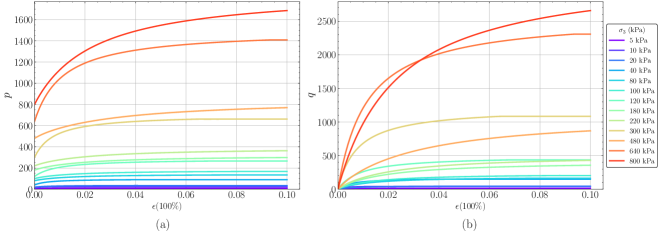
Figure 6: Representative stress-strain curves from simulated CD triaxial tests on sand specimens using the hardening soil model: (a) mean effective stress ($p$) versus axial strain ($\epsilon$) in %; (b) deviatoric stress ($q$) versus axial strain ($\epsilon$) in %, illustrating the response under varying confining pressures.

The simulation dataset consisted of 78 stress-strain-volume-change series (each test having $N=100$ samples) having confining pressures of 5, 10, 20, 40, 80, 100, 120, 180, 220, 300, 480, 640, and 800 kPa. These pressures cover a wide range from low to high-pressure regimes to ensure a diverse representation of stress states while maintaining computational efficiency. In triaxial tests, axial strain is typically expressed as a percentage of the initial sample height, with $N$ representing the total number of strain increments required to achieve the target strain. For a given triaxial experiment $(m)$, $N$ may vary depending on the total strain target. In this study, all the $M=78$ simulated triaxial tests had a $N=100$ number of strain increments with a max strain of 10%, consistent with typical experimental setups. Representative stress-strain series, showing variations in mean effective stress ($p$) and deviatoric stress ($q$) with axial strain ($\epsilon$), are illustrated in Fig.˜6.

The dataset was strategically split into three parts: the training set included confining pressures from 20–480 kPa, covering the midrange of confining pressure, while the validation set covered confining pressures at 10 kPa and 640 kPa, aimed at fixing the model hyperparameters to perform well beyond training range, and finally the test set was designed to cover confining pressures at 5 kPa and 800 kPa to evaluate model extrapolation performance under extreme low- and high-confining pressure scenarios.

The rFFFN and rBNN models were trained using a sliding window approach, wherein the window length $H$ was systematically varied from $H=2$ to $H=11$ to assess how the window size influenced model fitting and prediction accuracy. For the rFFNN, the validation results indicated that an optimal window length of $H=10$ minimized both RMSE and MAE, which exhibited consistent trends across all tested configurations (see Fig.˜7(a)).

For the rBNN, window length evaluation incorporated both RMSE, which measures prediction accuracy, and negative log-likelihood (NLL), which assesses uncertainty quantification. A window length of $H=7$ was chosen based on the combined minimization of RMSE and NLL, as shown in Fig.˜7(b). Lower NLL values indicate better calibration of uncertainty estimates and alignment with observed data.

At $H=1$, the rFFNN reduces to a standard FFNN without any recursive feedback. All window lengths $H\in\left[1,11\right]$ were comprehensively evaluated to ensure robust optimization for both the deterministic rFFNN and the probabilistic rBNN.

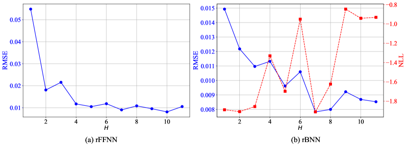
Figure 7: Selection of $H$ using the validation set of simulated case study: (a) RMSE variation with window length $H$ for rFFNN; (b) RMSE and NLL variation with $H$ for rBNN.

The training of the rBNN model was implemented in TensorFlow Probability [63], and used the negative ELBO loss function (Eq.˜19) for variational inference. Monte Carlo sampling was applied to propagate parameter uncertainties and construct the predictive distribution, as detailed in Section˜3.3.

For benchmarking, deterministic models such as LSTM, Bi-LSTM, GRU, FFNN, and rFFNN were trained with optimal hyperparameters identified through grid search by minimizing the RMSE and MAE on the validation set. The Huber loss function was adopted for these models. All models employed ReLU activation functions and the Adam optimizer [64], with an exponential learning rate scheduler to enhance training stability. Hyperparameters, including the number of layers, neurons per layer, and learning rates, were fine-tuned to minimize validation loss while ensuring stability.

Details of the architectures and training losses for the models are provided in Table˜1, with further implementation specifics for LSTM, Bi-LSTM, and GRU outlined in A. The performance metrics on the test set highlight the superior accuracy and uncertainty quantification capabilities of rBNN compared to deterministic models.

Table 1: Architecture and training configurations for models trained on simulated data.

Model Hidden Layers Neurons/Layer Training Loss Activation LSTM 2 100 Huber ReLU Bi-LSTM 3 100 Huber ReLU GRU 2 100 Huber ReLU FFNN ($H=1$) 2 125 Huber ReLU rFFNN ($H=10$) 2 115 Huber ReLU rBNN ($H=7$) 3 100 $-$ ELBO (Eq.˜19) ReLU

For the rBNN, a three-layer architecture with 100 neurons per layer was selected. Other models were configured with varying numbers of layers and neurons to ensure optimal performance across validation metrics.

The performance of the models on the test set is summarized in Table˜2. Both rFFNN and rBNN demonstrated superior accuracy, with rBNN achieving the lowest RMSE and MAE values for most state parameters ($p$, $q$, and $e$), outperforming all other models. The next best-performing models were rFFNN and Bi-LSTM.

While RMSE emphasizes sensitivity to larger prediction errors, MAE captures average absolute prediction deviations. RMSE values were consistently higher than MAE, indicating lower overfitting tendencies but slightly larger squared errors in predictions. The visual comparison of the predicted state parameters under extreme confining pressures (5 kPa and 800 kPa) in Figs.˜8, 9 and 10 further illustrates the model performance.

Unlike deterministic models, the rBNN provides confidence intervals for its predictions, quantifying the associated uncertainty. These confidence intervals closely encompass the true CD stress-strain responses, demonstrating the robustness of the rBNN in uncertainty quantification. This capability is particularly critical for decision-making in applications requiring confidence-aware predictions.

Table 2: Comparison of RMSE and MAE on the test set for DL models in the simulated dataset case, with bold values indicating the best performance for each parameter ($p$, $q$, $e$).

Models $p$ $q$ $e$ MAE RMSE MAE RMSE MAE RMSE LSTM 0.0032 0.0079 0.0127 0.0175 0.0056 0.0072 Bi-LSTM 0.0029 0.0051 0.0113 0.0132 0.0051 0.0057 GRU 0.0044 0.0070 0.0147 0.0184 0.0073 0.0124 FFNN($H$=1) 0.0058 0.0079 0.0152 0.0202 0.0132 0.0158 rFFNN($H$=10) 0.0032 0.0044 0.0109 0.0124 0.0046 0.0061 rBNN($H$=7) 0.0026 0.0039 0.0104 0.0125 0.0038 0.0054

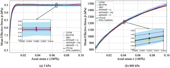
Figure 8: Comparison of predicted mean effective stress change versus axial strain for test set at extreme confining pressures: (a) 5 kPa (left) and (b) 800 kPa (right) in the simulated dataset case.

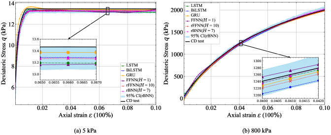
Figure 9: Comparison of predicted deviatoric stress change versus axial strain for test set at extreme confining pressures: (a) 5 kPa (left) and (b) 800 kPa (right) in the simulated dataset case.

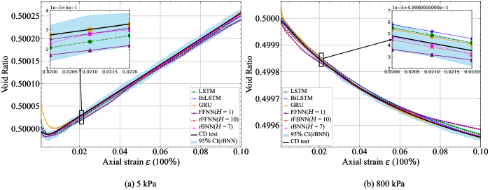
Figure 10: Comparison of predicted void ratio change versus axial strain for test set at extreme confining pressures: (a) 5 kPa (left) and (b) 800 kPa (right) in the simulated dataset case.

4.2 Evaluation on experimental data

The laboratory dataset used in this study comprises 28 CD triaxial tests conducted on Baskarp sand specimens at the University of Aalborg, as reported in [65]. These tests span three distinct initial void ratios ($e_{0}$): 0.85, 0.70, and 0.61, and nine different initial confining pressures ($\sigma_{3}$), ranging from 5 to 800 kPa. Soil samples were subjected to axial strains up to maximum values between 12% and 19% of the initial sample height, depending upon the specific test conditions.

For model training and evaluation, the dataset was split into two subsets: approximately 80% of the data was assigned for training, and the remaining 20% was used for testing. Due to the limited size of the dataset, no separate validation set was allocated. The training set primarily included midrange pressures (10–640 kPa), while the test set was designed to include extreme low- and high-confining pressures (5 kPa and 800 kPa) to assess the model’s extrapolation capabilities.

The preprocessing steps applied to the experimental dataset mirror those described for the simulated dataset (Section˜4.1). Stress invariants (mean effective stress $p$ and deviatoric stress $q$) and void ratios were normalized to ensure numerical stability and facilitate effective model training. Representative experimental stress-strain curves illustrating the evolution of $p$ and $q$ with axial strain $(\epsilon)$ under varying confining pressures are shown in Fig.˜11.

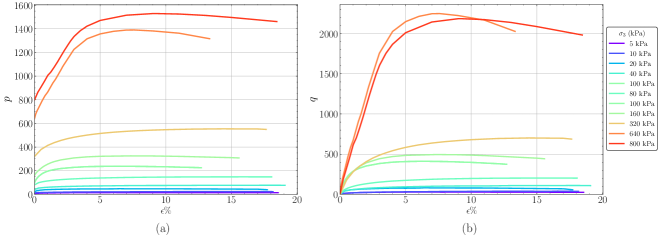
Figure 11: Representative stress-strain curves from experimental CD triaxial tests on Baskarp sand specimens done at University of Aalborg [65] : (a) mean effective stress ($p$) versus axial strain ($\epsilon$) in %; (b) deviatoric stress ($q$) versus axial strain ($\epsilon$) in %, illustrating the response under varying confining pressures.

The training process for the experimental dataset followed the methodology outlined for the simulated dataset (Section˜4.1). Deterministic models, including LSTM, Bi-LSTM, GRU, FFNN, and rFFNN, were trained using the Huber loss function, while the rBNN employed the negative ELBO loss function (Eq.˜19) for variational inference. Due to the absence of a validation set, hyperparameters, including the sliding window length $H$, were selected based on test set performance.

For the experimental data, $H=8$ was determined to be optimal for both rFFNN and rBNN, based on RMSE and NLL. The RMSE variation with window length for rFFNN and rBNN is illustrated in Fig.˜12. Model architectures and training configurations are summarized in Table˜3. All models employed ReLU activation functions and were trained using the Adam optimizer with learning rate scheduling. For rBNN, Monte Carlo sampling was utilized to propagate parameter uncertainties, enabling confidence intervals for predictions, a feature absent in deterministic models.

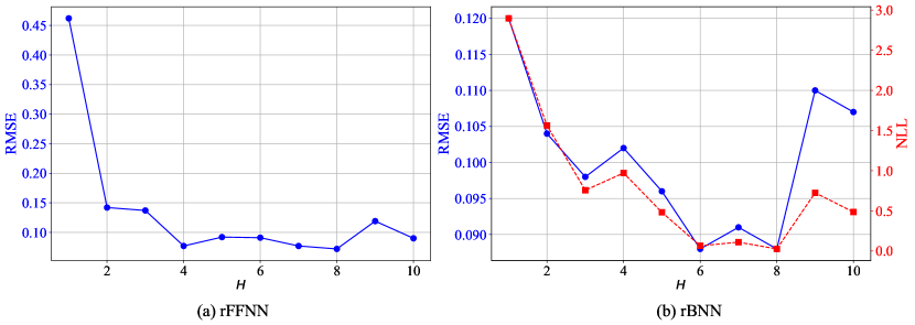
Figure 12: Selection of $H$ using test set of experimental case study: (a) RMSE variation with window length $H$ for rFFNN; (b) RMSE and NLL variation with $H$ for rBNN.

Table 3: Architecture and training configurations for models trained on experimental data.

Model Hidden Layers Neurons/Layer Training Loss Activation LSTM 2 100 Huber ReLU Bi-LSTM 2 100 Huber ReLU GRU 2 100 Huber ReLU FFNN 2 115-110 Huber ReLU rFFNN ($H=8$) 2 115-110 Huber ReLU rBNN ($H=8$) 2 115-110 $-$ ELBO (Eq.˜19) ReLU

The evaluation framework and performance metrics (MAE and RMSE) for the experimental dataset align with those used for the simulated dataset. The test set results for each state parameter $(p,q,e)$ are summarized in Table˜4. rFFNN achieved the best overall performance, with the lowest RMSE and MAE for $p$ and $q$, while rBNN achieved the lowest MAE score in predicting $e$. However, the rBNN does not outperform LSTM, Bi-LSTM, and rFFNN for the mean effective stress ($p$) and deviatoric stress ($q$).

A possible reason for the poorer performance of rBNN could be the limited size of the experimental dataset. With only 28 CD triaxial tests available, the amount of data may have been insufficient to properly constrain the posterior distribution of the model parameters, leading to inflated confidence intervals, as seen in the Figs.˜13, 14 and 15. . This is in contrast to the simulated dataset, where the larger dataset size (78 tests) allowed the rBNN to perform competitively and produce tighter confidence intervals.

These observations highlight the potential need for additional experimental data or strategies like data augmentation, transfer learning from simulated datasets, or more robust priors in the Bayesian framework to improve the performance of rBNN models in small datasets.

These results suggest that rBNN can offer competitive performance while providing probabilistic insights, particularly when sufficient data or advanced regularization strategies are applied. Despite its limitations in small datasets, the rBNN framework remains promising, with the potential for significant improvements when combined with techniques like transfer learning, robust priors, or enhanced data preprocessing.

Table 4: Performance metrics on test set for DL models trained on experimental data, with bold values indicating the best performance for each parameter ($p$, $q$, $e$).

Models $p$ $q$ $e$ MAE RMSE MAE RMSE MAE RMSE LSTM 0.0516 0.0747 0.0946 0.1312 0.0309 0.0467 Bi-LSTM 0.0522 0.0701 0.1023 0.1334 0.0277 0.0428 GRU 0.0792 0.0991 0.1449 0.1801 0.0641 0.0987 FFNN 0.0678 0.0853 0.1064 0.1329 0.0367 0.0508 rFFNN ($H=8$) 0.0494 0.0671 0.0754 0.1069 0.0228 0.0336 rBNN ($H=8$) 0.0564 0.0791 0.0973 0.1298 0.0225 0.0383

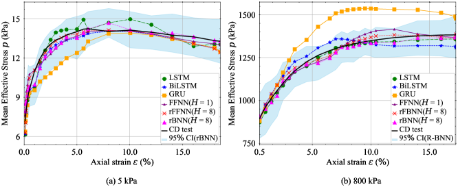
Figure 13: Comparison of predicted mean effective stress change versus axial strain for test set at extreme confining pressures: (a) 5 kPa (left) and (b) 800 kPa (right) in the experimental dataset case.

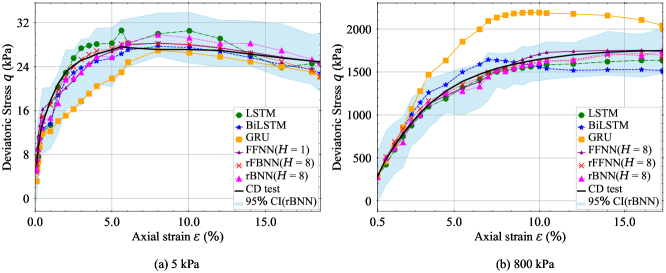
Figure 14: Comparison of predicted deviatoric stress change versus axial strain for test set at extreme confining pressures: (a) 5 kPa (left) and (b) 800 kPa (right)in the experimental dataset case.

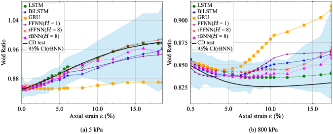
Figure 15: Comparison of predicted void ratio change versus axial strain for test set at extreme confining pressures: (a) 5 kPa (left) and (b) 800 kPa (right) in the experimental dataset case.

4.3 Computational time

The computational performance of the DL models was analyzed using hardware consisting of a MacBook Air with the M1 chip, equipped with an 8-core CPU and a 7-core GPU. The training environment was set up using Python 3.9.19, TensorFlow 2.15.0, PyTorch 1.11.0, and other necessary libraries. The training times for different deep learning models on simulated and experimental data are presented in Figs.˜16(a) and 16(b), respectively.

Models like LSTMs and Bi-LSTMs had the highest number of parameters, exceeding 100,000, due to their complex recurrent architectures. This parameter-heavy nature resulted in longer per-epoch training times compared to simpler models like rFFNN and rBNN. Despite their larger size, LSTMs and Bi-LSTMs demonstrated relative efficiency by achieving convergence within fewer iterations, balancing their computational demands.

In contrast, rFFNNs and rBNNs, which have significantly fewer parameters, demonstrated shorter overall training times on simulated data due to their simpler architectures. However, rBNN required the longest total training time on the experimental dataset. This extended training time is attributed to the computational complexity of Bayesian inference –specifically the reliance on Monte Carlo sampling to approximate posterior distributions – and the slow convergence due to a smaller dataset. Nonetheless, rBNN’s Bayesian framework enables it to provide predictive uncertainty through confidence intervals, a critical feature absent in deterministic models.

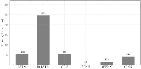
(a) Simulated dataset

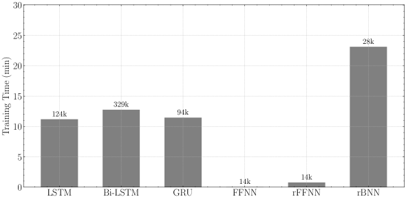
(b) Experimental dataset

Figure 16: Comparison of computational training times for different DL models: (a) models trained on simulated data, and (b) on experimental data. In both subfigures, the model sizes (i.e., the number of parameters) are indicated at the top of each bar in the bar graph.

For the simulated case study, Bi-LSTM required the longest training duration due to its bidirectional processing and extensive parameterization. For experimental data, rBNN took the longest, reflecting the additional computational load from Bayesian inference.

These findings underscore the distinct computational trade-offs across the models. LSTMs and Bi-LSTMs demonstrate faster convergence but require significant computational resources, making them suitable for cases where training efficiency is prioritized. Conversely, rFFNNs and rBNNs offer computational efficiency due to their simpler architectures, with rBNN providing the added benefit of uncertainty quantification. While rBNN required the longest training time on experimental data, its ability to quantify predictive uncertainty justifies the additional computational cost, particularly in applications where prediction reliability is critical.

4.4 Key takeaways from performance assessment

The performance evaluation section highlights several key observations and insights from both the simulated and experimental dataset case studies, as well as the computational time comparisons:

1. Performance of rFFNN and rBNN across datasets:

   • Simulated dataset: The rBNN demonstrated competitive performance, achieving the lowest RMSE and MAE for most state parameters ($p$, $q$, and $e$). The rFFNN also performed well, showing comparable accuracy to rBNN but with a simpler deterministic recursive framework.

   • Experimental dataset: In this dataset, the rFFNN consistently outperformed rBNN, achieving the best RMSE and MAE metrics for most state parameters. The inflated confidence intervals in rBNN’s predictions for experimental data suggest challenges in uncertainty calibration, likely due to the smaller dataset size and higher variability in experimental conditions.

2. Optimal window length: Both rFFNN and rBNN achieved their best performance at specific window lengths ($H=10$ for rFFNN and $H=7$ for rBNN on simulated data, and $H=8$ for both on experimental data), emphasizing the importance of tuning this hyperparameter to account.

3. Computational Efficiency: The rFFNN and rBNN models required significantly fewer trainable parameters compared to LSTMs and Bi-LSTMs. The rFFNN results in faster training times, while rBNN takes longer times (comparable to LSTMs) due to the sampling framework. The cost of the higher training time is compensated by the output uncertainty provided by the framework.

5 Discussion

This study highlights the potential of recursive neural network architectures, particularly rFFNNs and rBNNs, in modeling the constitutive behavior of sand under monotonic loading conditions, emphasizing both predictive accuracy and uncertainty quantification. Unlike recurrent models such as LSTMs and GRUs, which rely on hidden states and gating mechanisms, rFFNNs provide a transparent and interpretable mapping between input features and output states across load steps. This transparency enhances their utility in analyzing the impact of specific input features on the predicted state variables, making rFFNNs and their Bayesian counterpart (rBNNs) valuable tools in geotechnical modeling.

One distinguishing feature of rFFNNs and rBNNs is the use of a sliding window length $H$, which defines the temporal context for training and recursive predictions. Unlike LSTMs or GRUs, which inherently model sequential dependencies through hidden states, rFFNNs and rBNNs require an explicit window length. The choice of $H$ plays a significant role in balancing predictive performance and computational efficiency, as demonstrated in this study.

From a performance perspective, the deterministic rFFNN consistently outperforms probabilistic rBNNs and other recurrent models, such as LSTMs and Bi-LSTMs, across various metrics for both simulated and experimental data. Their simplicity and efficiency allow them to achieve superior accuracy when sufficient training data is available. However, the rBNN provides an essential advantage in uncertainty quantification, producing confidence intervals that account for uncertainties. This feature is particularly beneficial in geotechnical applications where predictive confidence is critical for risk assessment.

On experimental datasets, the rBNN’s performance lags slightly behind deterministic models in terms of root mean square error (RMSE) and mean absolute error (MAE), especially for the stress components ($p$ and $q$). The inflated confidence intervals observed in experimental data highlight the challenges posed by data sparsity and measurement noise, as opposed to simulated datasets where these factors are controlled. This suggests that the rBNN’s probabilistic framework, while robust, requires careful calibration and potentially enhanced priors or noise models to improve its representation of experimental variability.

A promising avenue for future work is the exploration of Bayesian LSTMs. These models combine the sequential modeling capabilities of LSTMs with Bayesian principles, allowing them to handle long-term dependencies while capturing both predictive uncertainties and epistemic uncertainties in model parameters. Bayesian LSTMs could address some of the limitations observed in rBNNs, particularly for experimental datasets where sequential dependencies and noise in measurements play a larger role.

6 Conclusion

This study underscores the utility of recursive architectures in advancing constitutive modeling for sands, bridging the gap between predictive performance and uncertainty quantification. The rFFNN excels in deterministic accuracy, offering a reliable tool for direct predictions, while the rBNN’s probabilistic framework provides valuable insights into prediction confidence, albeit at a computational cost.

Future research directions include integrating enhanced priors and noise models to improve the rBNN’s performance with sparse experimental data, as well as exploring hybrid frameworks that combine deterministic and probabilistic components. Additionally, efforts should focus on optimizing computational efficiency, particularly for Bayesian models, to enable their broader adoption in large-scale geotechnical applications.

CRediT authorship contribution statement

Toiba Noor: Conceptualization, Methodology, Software, Writing - original draft. Soban Nasir Lone: Methodology, Software, Writing - review & editing. G.V. Ramana: Supervision, Writing - review & editing. Rajdip Nayek: Conceptualization, Supervision, Methodology, Writing - review & editing.

Declaration of Competing Interest

The authors declare that they have no known competing financial interests or personal relationships that could have appeared to influence the work reported in this paper.

Appendix A Training and Optimization of RNNs

The data normalization process for RNNs mirrors the approach used for rFFNN and rBNN. Models across the RNN family, including LSTM, Bi-LSTM, and GRU, utilize the same data preparation strategy for both simulated and experimental datasets. The RNN models were trained using input data structured as shown in Fig.˜17, with a feedback framework described by:

Figure 17: Illustration of the data structure used for Recurrent Neural Networks.

$$\bm{{s}}_{t}^{(m)}=f\left(\bm{{s}}_{t-1}^{(m)},\bm{{u}}_{t}^{(m)},\bm{{\theta}}^{(m)}\right)$$ (33)

For simulated data, hyperparameters of each RNN model were systematically tuned to achieve optimal performance in the validation set. The hyperparameter space for LSTM included learning rates ($0.0001$ to $0.01$), number of LSTM layers ($1$ to $4$), and number of nodes in each layer ($50$ to $200$). Batch sizes ($1$ to $25$) were validated to balance computational efficiency and gradient stability. The suitability of the Huber loss function over MSE loss was evaluated based on validation loss. Optimization algorithms, including Adam and RMSprop, were also validated. The number of epochs ranged from $1000$ to $10000$, and model selection was guided by Total MSE of the validation set to ensure robust generalization. A similar systematic approach was applied for Bi-LSTM and GRU models, with final details of the architecture summarized in Table˜1.

For experimental datasets, hyperparameter tuning followed an identical systematic approach, validating combinations to ensure consistency across the models, with final details of the architecture summarized in Table˜3 .

These models were trained by calculating losses for predictions made at each strain increment, strictly adhering to the feedback framework outlined in Fig.˜17. While the feedback framework primarily predicts the current state using only the immediately preceding state, the approach can be extended to incorporate multiple previous states to enhance the capture of temporal dependencies in the data i.e., the input window can have multiple consecutive load steps of the input states that helps predict the output state. For example, when using three input load steps, as shown in Eq.˜34, the RNNs utilized sequences of $p$, $q$, $e$, $\epsilon$, and $d\epsilon$ from the past three load steps:

$$=f\left(\begin{bmatrix}\bm{{s}}_{t-3}^{(m)}&\bm{{u}}_{t-2}^{(m)}\\ \bm{{s}}_{t-2}^{(m)}&\bm{{u}}_{t-1}^{(m)}\\ \bm{{s}}_{t-1}^{(m)}&\bm{{u}}_{t}^{(m)}\end{bmatrix},\bm{{\theta}}^{(m)}\right)$$ (34)

While this approach effectively captures temporal dependencies, it necessitates the availability of the atleast, in this case, the first three state parameters during testing, which are often unavailable. Consequently, its practical applicability is limited in scenarios where these initial parameters cannot be obtained.

References

- Hong et al. [2017] Yi Hong, Chi Hung Koo, Chao Zhou, Charles WW Ng, and LZ Wang. Small strain path-dependent stiffness of toyoura sand: Laboratory measurement and numerical implementation. International Journal of Geomechanics, 17(1):1–10, 2017.
- Secondi et al. [2013] Marco M Secondi, Giovanni Crosta, Claudio di Prisco, Gabriele Frigerio, Paolo Frattini, and Federico Agliardi. Landslide motion forecasting by a dynamic visco-plastic model. Landslide Science and Practice: Volume 3: Spatial Analysis and Modelling, pages 151–159, 2013.
- Desai et al. [1995] Chandra S Desai, Naresh C Samtani, and Laurent Vulliet. Constitutive modeling and analysis of creeping slopes. Journal of Geotechnical Engineering, 121(1):43–56, 1995.
- Hejazi et al. [2008] Yousef Hejazi, Daniel Dias, and Richard Kastner. Impact of constitutive models on the numerical analysis of underground constructions. Acta Geotechnica, 3:251–258, 2008.
- Gäb et al. [2008] Martin Gäb, Helmut F Schweiger, Daniela Kamrat-Pietraszewska, and Minna Karstunen. Numerical analysis of a floating stone column foundation using different constitutive models. In Geotechnics of Soft Soils: Focus on Ground Improvement, pages 149–154. CRC Press, 2008.
- Rychlewski [1984] Jan Rychlewski. On Hooke’s law. Journal of Applied Mathematics and Mechanics, 48(3):303–314, 1984.
- Makris and Constantinou [1993] Nicos Makris and MC Constantinou. Models of viscoelasticity with complex-order derivatives. Journal of Engineering Mechanics, 119(7):1453–1464, 1993.
- Bardet [1992] JP Bardet. A viscoelastic model for the dynamic behavior of saturated poroelastic soils. Journal of Applied Mechanics, 59(1):128–135, 1992.
- Duncan and Chang [1970] James M Duncan and Chin Yung Chang. Nonlinear analysis of stress and strain in soils. Journal of the Soil Mechanics and Foundations Division, 96(5):1629–1653, 1970.
- Yao et al. [2019] Yang-Ping Yao, Lin Liu, Ting Luo, Yu Tian, and Jian-Min Zhang. Unified hardening model for clays and sands. Computers and Geotechnics, 110:326–343, 2019.
- Cassiani et al. [2017] G Cassiani, A Brovelli, and T Hueckel. A strain-rate-dependent modified Cam-Clay model for the simulation of soil/rock compaction. Geomechanics for Energy and the Environment, 11:42–51, 2017.
- Drucker and Prager [1952] Daniel Charles Drucker and William Prager. Soil mechanics and plastic analysis or limit design. Quarterly of Applied Mathematics, 10(2):157–165, 1952.
- Yin et al. [2020a] Zhen-Yu Yin, Pierre-Yves Hicher, Yin-Fu Jin, Zhen-Yu Yin, Pierre-Yves Hicher, and Yin-Fu Jin. Elastoplastic modeling of soils: From Mohr-Coulomb to SIMSAND. Practice of Constitutive Modelling for Saturated Soils, pages 121–176, 2020a.
- Schanz and Vermeer [1996] T Schanz and PA Vermeer. Angles of friction and dilatancy of sand. Géotechnique, 46(1):145–151, 1996.
- Yang and Li [2004] Jinglin Yang and XS Li. State-dependent strength of sands from the perspective of unified modeling. Journal of Geotechnical and Geoenvironmental Engineering, 130(2):186–198, 2004.
- Wu [1998] Wei Wu. Rational approach to anisotropy of sand. International Journal for Numerical and Analytical Methods in Geomechanics, 22(11):921–940, 1998.
- Jardine et al. [1986] RJ Jardine, DM Potts, AB Fourie, and JB Burland. Studies of the influence of non-linear stress–strain characteristics in soil–structure interaction. Geotechnique, 36(3):377–396, 1986.
- Benz et al. [2008] T Benz, M Wehnert, and PA Vermeer. A lode angle dependent formulation of the hardening soil model. In The 12th International Conference of International Association for Computer Methods and Advances in Geomechanics (IACMAG), pages 1–6, 2008.
- Cameron and Carter [2009] Donald A Cameron and John P Carter. A constitutive model for sand based on non-linear elasticity and the state parameter. Computers and Geotechnics, 36(7):1219–1228, 2009.
- Jefferies [1993] MG Jefferies. Nor-sand: A simple critical state model for sand. Géotechnique, 43(1):91–103, 1993.
- Gajo and Wood [1999] Alessandro Gajo and Muir Wood. Severn–Trent sand: A kinematic-hardening constitutive model: The q–p formulation. Géotechnique, 49(5):595–614, 1999.
- Taiebat and Dafalias [2008] Mahdi Taiebat and Yannis F Dafalias. SANISAND: Simple anisotropic sand plasticity model. International Journal for Numerical and Analytical Methods in Geomechanics, 32(8):915–948, 2008.
- Yin et al. [2017] Zhen-Yu Yin, Pierre-Yves Hicher, Christophe Dano, and Yin-Fu Jin. Modeling mechanical behavior of very coarse granular materials. Journal of Engineering Mechanics, 143(1), 2017.
- Yin et al. [2020b] Zhen-Yu Yin, Pierre-Yves Hicher, Yin-Fu Jin, Zhen-Yu Yin, Pierre-Yves Hicher, and Yin-Fu Jin. Viscoplastic modeling of soft soils. Practice of Constitutive Modelling for Saturated Soils, pages 229–271, 2020b.
- Wu et al. [2017] Wei Wu, Jia Lin, and Xuetao Wang. A basic hypoplastic constitutive model for sand. Acta Geotechnica, 12:1373–1382, 2017.
- Yin et al. [2010] Zhen-Yu Yin, Ching S Chang, and Pierre-Yves Hicher. Micromechanical modelling for effect of inherent anisotropy on cyclic behaviour of sand. International Journal of Solids and Structures, 47(14-15):1933–1951, 2010.
- Yin and Jin [2019] Zhen Yu Yin and Yin Fu Jin. Practice of optimisation theory in geotechnical engineering. Springer Singapore, Singapore, April 2019. ISBN 9789811334078. Publisher Copyright: © 2022 Springer Nature Switzerland AG. Part of Springer Nature.
- Herle [2021] Ivo Herle. Fundamentals of constitutive modelling for soils. ALERT Doctoral School 2021 Constitutive Modelling in Geomaterials, page 3, 2021.
- Zhang et al. [2021a] Pin Zhang, Zhen-Yu Yin, and Yin-Fu Jin. State-of-the-art review of machine learning applications in constitutive modeling of soils. Archives of Computational Methods in Engineering, pages 1–26, 2021a.
- Ellis et al. [1992] Glenn W Ellis, Chengwan Yao, and Rongda Zhao. Neural network modeling of the mechanical behavior of sand. In Engineering Mechanics, pages 421–424. ASCE, 1992.
- Ellis et al. [1995] GW Ellis, C Yao, Rui Zhao, and Df Penumadu. Stress-strain modeling of sands using artificial neural networks. Journal of Geotechnical Engineering, 121(5):429–435, 1995.
- Sidarta and Ghaboussi [1998] DE Sidarta and J Ghaboussi. Constitutive modeling of geomaterials from non-uniform material tests. Computers and Geotechnics, 22(1):53–71, 1998.
- Penumadu and Zhao [1999] Dayakar Penumadu and Rongda Zhao. Triaxial compression behavior of sand and gravel using artificial neural networks. Computers and Geotechnics, 24(3):207–230, 1999.
- Habibagahi and Bamdad [2003] Ghassem Habibagahi and Alireza Bamdad. A neural network framework for mechanical behavior of unsaturated soils. Canadian Geotechnical Journal, 40(3):684–693, 2003.
- Najjar and Zhang [2000] Yacoub Najjar and Xiaobin" Carol" Zhang. Characterizing the 3D stress-strain behavior of sandy soils: A neuro-mechanistic approach. In Numerical methods in Geotechnical Engineering, volume 24, pages 43–57. Elsevier, 2000.
- Ghaboussi and Sidarta [1998] Jamshid Ghaboussi and Djoni Eka Sidarta. New nested adaptive neural networks for constitutive modeling. Computers and Geotechnics, 22(1):29–52, 1998.
- Zhu et al. [1998] Jian-Hua Zhu, Musharraf M Zaman, and Scott A Anderson. Modeling of soil behavior with a recurrent neural network. Canadian Geotechnical Journal, 35(5):858–872, 1998.
- Najjar and Ali [1999] YM Najjar and HE Ali. Simulating the stress-strain behavior of Nevada sand by Artificial Neural Networks. In Proceedings of the 5th US National Congress on Computational Mechanics (USACM), Boulder, Colorado, pages 0–1, 1999.
- Romo et al. [2001] Miguel P Romo, Silvia R García, Manuel J Mendoza, and Victor Taboada-Urtuzuástegui. Recurrent and constructive-algorithm networks for sand behavior modeling. International Journal of Geomechanics, 1(4):371–387, 2001.
- Hochreiter and Schmidhuber [1997] Sepp Hochreiter and Jürgen Schmidhuber. Long short-term memory. Neural Computation, 9(8):1735–1780, 1997.
- Chung et al. [2014] Junyoung Chung, Caglar Gulcehre, Kyunghyun Cho, and Yoshua Bengio. Empirical evaluation of gated recurrent neural networks on sequence modeling. In NIPS 2014 Workshop on Deep Learning, December, 2014.
- Zhang et al. [2020] Pin Zhang, Zhen-Yu Yin, Yin-Fu Jin, and Guan-Lin Ye. An AI-based model for describing cyclic characteristics of granular materials. International Journal for Numerical and Analytical Methods in Geomechanics, 44(9):1315–1335, 2020.
- Zhang et al. [2021b] Ning Zhang, Shui-Long Shen, Annan Zhou, and Yin-Fu Jin. Application of LSTM approach for modelling stress–strain behaviour of soil. Applied Soft Computing, 100:106959, 2021b.
- Qu et al. [2021] Tongming Qu, Shaocheng Di, YT Feng, Min Wang, Tingting Zhao, and Mengqi Wang. Deep learning predicts stress–strain relations of granular materials based on triaxial testing data. Computer Modeling in Engineering & Sciences, 128(1):129–144, 2021.
- Wu et al. [2023] Mengmeng Wu, Zhangqi Xia, and Jianfeng Wang. Constitutive modelling of idealised granular materials using machine learning method. Journal of Rock Mechanics and Geotechnical Engineering, 15(4):1038–1051, 2023.
- MacKay [1995] David JC MacKay. Probable networks and plausible predictions- A review of practical Bayesian methods for supervised neural networks. Network: Computation in Neural Systems, 6(3):469, 1995.
- Neal [2012] Radford M Neal. Bayesian learning for neural networks, volume 118. Springer Science & Business Media, 2012.
- Jospin et al. [2022] Laurent Valentin Jospin, Hamid Laga, Farid Boussaid, Wray Buntine, and Mohammed Bennamoun. Hands-on Bayesian neural networks—A tutorial for deep learning users. IEEE Computational Intelligence Magazine, 17(2):29–48, 2022.
- Knoblauch et al. [2022] Jeremias Knoblauch, Jack Jewson, and Theodoros Damoulas. An optimization-centric view on Bayes’ rule: Reviewing and generalizing variational inference. Journal of Machine Learning Research, 23(132):1–109, 2022. URL http://jmlr.org/papers/v23/19-1047.html.
- Ghosh and Basu [2016] Abhik Ghosh and Ayanendranath Basu. Robust Bayes estimation using the density power divergence. Annals of the Institute of Statistical Mathematics, 68:413–437, 2016.
- Guedj [2019] Benjamin Guedj. A primer on pac-Bayesian learning. arXiv preprint arXiv:1901.05353, 2019.
- Pham et al. [2022] Khanh Pham, Sanghoon Jung, Sangyeong Park, Dongku Kim, and Hangseok Choi. Bayesian neural network for estimating stress-strain behaviors of frozen sand. KSCE Journal of Civil Engineering, 26(2):933–941, 2022.
- Gal and Ghahramani [2016] Yarin Gal and Zoubin Ghahramani. Dropout as a Bayesian approximation: Representing model uncertainty in deep learning. In International Conference on Machine Learning, pages 1050–1059. PMLR, 2016.
- Zhang et al. [2023] Pin Zhang, Zhen-Yu Yin, and Brian Sheil. Interpretable data-driven constitutive modelling of soils with sparse data. Computers and Geotechnics, 160:105511, 2023.
- Fortuin [2022] Vincent Fortuin. Priors in Bayesian deep learning: A review. International Statistical Review, 90(3):563–591, 2022.
- Matsubara et al. [2022] Takuo Matsubara, Jeremias Knoblauch, François-Xavier Briol, and Chris J Oates. Robust generalised Bayesian inference for intractable likelihoods. Journal of the Royal Statistical Society Series B: Statistical Methodology, 84(3):997–1022, 2022.
- Kucukelbir et al. [2017] Alp Kucukelbir, Dustin Tran, Rajesh Ranganath, Andrew Gelman, and David M Blei. Automatic differentiation variational inference. Journal of Machine Learning Research, 18(14):1–45, 2017.
- Kingma [2013] Diederik P Kingma. Auto-encoding variational bayes. arXiv preprint arXiv:1312.6114, 2013.
- Blundell et al. [2015] Charles Blundell, Julien Cornebise, Koray Kavukcuoglu, and Daan Wierstra. Weight uncertainty in neural network. In International Conference on Machine Learning, pages 1613–1622. PMLR, 2015.
- Knoblauch et al. [2019] Jeremias Knoblauch, Jack Jewson, and Theodoros Damoulas. Generalized variational inference: Three arguments for deriving new posteriors. arXiv preprint arXiv:1904.02063, 2019.
- Schanz et al. [1999] T Schanz, PA Vermeer, and P Gc Bonnier. The hardening soil model: Formulation and Verification. Beyond 2000 in Computational Geotechnics, 1:281–296, 1999.
- Wichtmann et al. [2017] T Wichtmann, I Kimmig, and T Triantafyllidis. On correlations between “dynamic”(small-strain) and “static”(large-strain) stiffness moduli–An experimental investigation on 19 sands and gravels. Soil Dynamics and Earthquake Engineering, 98:72–83, 2017.
- Dillon et al. [2017] Joshua V Dillon, Ian Langmore, Dustin Tran, Eugene Brevdo, Srinivas Vasudevan, Dave Moore, Brian Patton, Alex Alemi, Matt Hoffman, and Rif A Saurous. Tensorflow distributions. arXiv preprint arXiv:1711.10604, 2017.
- Alkroosh and Nikraz [2012] Iyad Alkroosh and Hamid Nikraz. Predicting axial capacity of driven piles in cohesive soils using intelligent computing. Engineering Applications of Artificial Intelligence, 25(3):618–627, 2012.
- Ibsen and Bødker [1994] Lars Bo Ibsen and Lars Bødker Bødker. Baskarp sand no. 15: Data report 9301. Aalborg: Geotechnical Engineering Group. Data Report, No. 9401, 1994.