Informativity Conditions for Multiple Signals: Properties, Experimental Design, and Applications

Abstract

Recent studies highlight the importance of persistently exciting condition in single signal sequence for model identification and data-driven control methodologies. However, maintaining prolonged excitation in control signals introduces significant challenges, as continuous excitation can reduce the lifetime of mechanical devices. In this paper, we introduce three informativity conditions for various types of multi-signal data, each augmented by weight factors. We explore the interrelations between these conditions and their rank properties in linear time-invariant systems. Furthermore, we introduce open-loop experimental design methods tailored to each of the three conditions, which can synthesize the required excitation conditions either offline or online, even in the presence of limited information within each signal segment. We demonstrate the effectiveness of these informativity conditions in least-squares identification. Additionally, all three conditions can extend Willems’ fundamental lemma and are utilized to assess the properties of the system. Illustrative examples confirm that these conditions yield satisfactory outcomes in both least-squares identification and the construction of data-driven controllers .

Informativity conditions, system identification, experiment design, linear time-invariant systems

1 Introduction

With the continuous development and application of data-driven technologies, the academic interest in data informativity has surged notably. In this context, the concept of persistently exciting (PE) condition [1] plays a crucial role. The PE condition requires that a signal be sufficiently rich over time to capture all dynamic characteristics of the system. This requirement is fundamental to various system identification methods [2, 3, 4, 5, 6] and data-driven control methods [7, 8, 9, 10, 11, 12]. However, although a single trajectory can theoretically satisfy the PE condition [13], due to experimental limitations such as the inability to apply filtered white noise excitation or the limited capacity of the controller, it may still be impossible to generate informative trajectories in practice. Consequently, designing data-driven techniques that do not rely on the stringent PE condition has become a critical issue that warrants significant attention.

Existing research has shown that PE condition is not a necessary prerequisite for system identification and data-driven control design [14, 15, 16]. In the domain of system identification, methods such as dynamic regressor extension and mixing [17, 18] have relaxed the PE condition by extending the regression model in the time domain. Certain adaptive methods [19] only require that excitation conditions be met during the initial phase. Furthermore, the challenge of insufficient information from a single sensor has been addressed through distributed frameworks [20, 21] and centralized frameworks [22]. Despite these advancements, these methods often relax the information content of system regression vectors or system trajectories, yet rarely focus on designing from the perspective of control signals. Therefore, a clear experimental design strategy for system input signals remains essential. While current experimental design theories are primarily based on the premise of satisfying identifiability [23, 24, 25, 26], there remains a significant gap in research regarding how to design experiments that guarantee the effectiveness of identification methods when the informativeness of input signals is lacking. In such cases, the use of multiple trajectories may be necessary.

In the design of data-driven control methods, A new control framework is developed in [14] that eliminates the stringent requirement of PE, but the trajectory data used still needs to guarantee the identifiability condition. The collectively persistently exciting (CPE) condition proposed in [27] and [28] offers potential insights for the design of data-driven control methods using trajectories generated by insufficiently informative controllers. By organizing the Hankel matrices that evaluate the excitability of each signal sequence side-by-side into a larger rank judgment matrix, this condition extends the fundamental lemma from a single signal sequence to multiple signal sequences. However, this large matrix structure can lead to a dramatic increase in computational burden as the number of columns increases, and excessive differences in the magnitude of the values between each Hankel matrix can also cause deviations from the expected results. Additionally, it is currently an open question how to provide more choices of matrix structures for different data-driven problems [29].

Motivated by the aforementioned challenges, the objective of this paper is to relax the PE condition typically required for a single control sequence in data-driven methods, while offering more flexible matrix structure choices for a variety of data-driven problems. Furthermore, we aim to design experimental methodologies that ensure the effectiveness of data-driven techniques even in scenarios where data informativeness is lacking. Specifically, the contributions of this paper are summarized as follows:

• We introduce three weighted CPE conditions for multiple signal sequences with different dimensions, same dimensions, and partially the same dimensions. All three conditions relax the PE condition requirement for a single signal sequence. Furthermore, we analyze the feasibility of implementing these conditions and their transformation relationships, and provide an initial exploration of which CPE conditions are most suitable for different problem types.

• For the three CPE conditions, we design experimental schemes and demonstrate that these experimental designs remain effective even when signal sequence information is insufficient. We also explore how control sequences satisfying the CPE conditions guide the convergence precision of least-squares (LS) estimators. Furthermore, by utilizing the three CPE conditions, we extend Willems’ fundamental lemma, and the extended lemma yields satisfactory results in data-driven control methods.

The remainder of this paper is organized as follows. Section 2 presents the preliminaries, including key definitions and a review of existing work on PE condition. Section 3 defines three CPE conditions related to data dimensions and explores their transformational relationships and rank properties. Section 4 introduces experimental methods tailored to the three CPE conditions and demonstrates their validity. Section 5 discusses the application of the CPE conditions to the least-squares (LS) identification method, and extends Willems’ fundamental lemma. Section 6 provides illustrative examples to validate the methodologies and theories discussed, while Section 7 concludes the paper.

2 Preliminaries

2.1 Notation

Throughout this paper, $\mathbb{Z}$, $\mathbb{N}$, $\mathbb{R}$ and $\mathbb{R}^{m\times n}$ denote the sets of integers, natural numbers, real numbers and $m\times n$ real matrices, respectively. $0_{m\times n}$ denotes a zero matrix with $m$ rows and $n$ columns. $\bm{1}_{n}$ represents the $n$-dimensional column vector with all entries set to one. $I_{n}$ and $0_{n}$ refer to the identity matrix and zero matrix of order $n$, respectively, without subscripts to indicate the suitable dimension. The modulo operation $\text{mod}(a,b)$ returns the remainder when $a$ is divided by $b$.

For a real matrix $P\in\mathbb{R}^{m\times n}$, let $P_{vec}=[P_{1},P_{2},\ldots,P_{m}]^{T}$, where $P_{i}$ represents the $i$-th row of $P$. The right kernel and left kernel of $P$ refer to the spaces of all real column vectors $v_{1}$ and row vectors $v_{2}$, respectively, satisfying $Pv_{1}=0$ and $v_{2}P=0$. The image, right kernel, left kernel, rank and Moore–Penrose pseudoinverse of $P$ are denoted as $\text{im}\,P$, $\text{ker}\,P$, $\text{leftker}\,P$, $\text{rank}\,P$ and $P^{{\dagger}}$, respectively. Additionally, let $\lambda_{max}(P)$, $||P||$, and $||P||_{2}$ represent the maximal eigenvalue, Frobenius norm, and spectral norm of $P$, respectively. Finally, let $\overline{\sigma}(P)$ and $\underline{\sigma}(P)$ denote the maximum singular value and minimum singular value of $P$, respectively.

Given a signal $z$: $\mathbb{Z}\rightarrow\mathbb{R}^{m}$, we define $z^{[k,k+T_{0}]}$ as

$$z^{[k,k+T_{0}]}=\begin{bmatrix}{z(k)}\\ \vdots\\ {z(k+{T_{0}})}\end{bmatrix},$$

where $k\in\mathbb{Z}$ and $T_{0}\in\mathbb{N}$. The block Hankel matrix of order $L$ associated to $z^{[k,k+T_{0}]}$ is defined as

$${H_{L}}({z^{[k,k+{T_{0}}]}})$$

$$~~=\begin{bmatrix}{z(k)}&{z(k+1)}&\cdots&{z(k+{T_{0}}-L+1)}\\ {z(k+1)}&{z(k+2)}&\cdots&{z(k+{T_{0}}-L+2)}\\ \vdots&\vdots&\ddots&\vdots\\ {z(k+L-1)}&{z(k+L)}&\cdots&{z(k+{T_{0}})}\end{bmatrix}.$$

2.2 Persistency of Excitation for a Single Sequence

The concept of persistency of excitation for a single signal sequence, as defined in [1], is elucidated below.

Definition 1

(Persistently Exciting Condition [1]). A signal sequence $z^{[0,T_{0}-1]}$ with $z(k)\in\mathbb{R}^{m}$, $k=0,...,T_{0}-1$ is PE of order $L$ if the block Hankel matrix $H_{L}(z^{[0,T_{0}-1]})$ has full row rank $mL$.

It is intuitive from this definition that a PE signal of order $L$ possesses the ability to span the entire real space $\mathbb{R}^{mL}$. In particular, if the input signal to a controllable linear time-invariant (LTI) system exhibits sufficiently high-order persistency of excitation, some attractive properties arise. Consider the LTI system

$$x(k+1)=Ax(k)+Bu(k),$$ (1)

where $A\in{\mathbb{R}^{n\times n}}$, ${B}\in{\mathbb{R}^{n\times{m}}}$, ${x(k)}\in{\mathbb{R}^{n}}$ and ${u(k)}\in{\mathbb{R}^{m}}$ represent the state vector and control input vector, respectively. The pair $(A,B)$ is controllable. A fundamental property in [1, Cor. 2] demonstrates that the LTI system (1) satisfies the rank condition

$$\text{rank}\,\begin{bmatrix}{{H_{1}}({x^{[0,{T_{0}}-L]}})}\\ {{H_{L}}({u^{[0,{T_{0}}-1]}})}\end{bmatrix}=n+mL$$ (2)

if the control input $u^{[0,{T_{0}}-1]}$ is PE of order $L+n$.

In addition, the rank condition (2) subtly implies that the sequences ${{{\bar{x}}^{[0,L-1]}}}$ and ${{{\bar{u}}^{[0,L-1]}}}$ form an $L$-long state-input trajectory of (1) if and only if there exists $g\in\mathbb{R}^{T_{0}-L+1}$ such that

$$\begin{bmatrix}{{{\bar{x}}^{[0,L-1]}}}\\ {{{\bar{u}}^{[0,L-1]}}}\end{bmatrix}=\begin{bmatrix}{{H_{L}}({x^{[0,{T_{0}}-1]}})}\\ {{H_{L}}({u^{[0,{T_{0}}-1]}})}\end{bmatrix}g.$$ (3)

This property indicates that the image of the matrix $\begin{bmatrix}{{H_{L}}({x^{[0,{T_{0}}-1]}})}\\ {{H_{L}}({u^{[0,{T_{0}}-1]}})}\end{bmatrix}$ is the representation of the $L$-long state-input trajectory space of the LTI system (1). It has been rigorously proved in the behavioral system framework [1, Th. 1] and the state-space framework [10, Lem. 2], respectively.

The properties described by (2) and (3), often referred to as Willems’ fundamental lemma due to their foundational importance for system identification and data-driven control.

Indeed, if the input sequence $u^{[0,{T_{0}}-1]}$ of system (1) is PE of order $n+1$, the matrix $\begin{bmatrix}{{H_{1}}({x^{[0,{T_{0}}-1]}})}\\ {{H_{1}}({u^{[0,{T_{0}}-1]}})}\end{bmatrix}$ has full row rank. This condition enables the recovery of the system matrices $A$ and $B$ from the data $x^{[0,{T_{0}}-1]}$ and $u^{[0,{T_{0}}-1]}$, i.e., identifiability condition (see [30, 14]). The system matrices can be uniquely determined by solving the following equation:

$$\begin{bmatrix}A&B\end{bmatrix}={H_{1}}({x^{[1,{T_{0}}]}}){\begin{bmatrix}{{H_{1}}({x^{[0,{T_{0}}-1]}})}\\ {{H_{1}}({u^{[0,{T_{0}}-1]}})}\end{bmatrix}^{\dagger}}.$$ (4)

On the other hand, under the influence of the prior control input $u^{[0,T_{0}-1]}$ that satisfies the PE condition, the system trajectories ${\bar{x}}^{[0,L-1]}$ and ${\bar{u}}^{[0,L-1]}$ can form the non-parametric representation in (3), which solely relies on the prior data. Consequently, in addition to its important role in system identification, PE condition has received widespread attention in the development of data-driven controllers such as parametric model reconstruction methods [10, 12] and data-driven model predictive control methods [7, 8, 9].

Even though it has been shown how to ensure the informativeness of a single control sequence [13], in some cases it may still not be possible to generate sufficiently informative trajectories due to the many limitations of the experiment. However, Designing experiments with insufficiently informative controllers fail to ensure the identifiability condition and the feasibility of data-driven approaches.

Example 1

When applying a feedback controller $u=Kx$, where $K$ is the control gain, we have

$${{H_{L}}({u^{[0,{T_{0}}-1]}})}=\begin{bmatrix}{K{{(A+BK)}^{0}}{H_{1}}({x^{[0,{T_{0}}-L]}})}\\ \vdots\\ {K{{(A+BK)}^{L-1}}{H_{1}}({x^{[0,{T_{0}}-L]}})}\end{bmatrix},$$

which means that every row of ${{H_{L}}({u^{[0,{T_{0}}-1]}})}$ is in the row space of ${H_{1}}({x^{[0,{T_{0}}-L]}})$. Therefore,

$$\text{rank}\ {{H_{L}}({u^{[0,{T_{0}}-1]}})}<mL.$$

Consequently,

$$\text{rank}\,\begin{bmatrix}{{H_{1}}({x^{[0,{T_{0}}-L]}})}\\ {{H_{L}}({u^{[0,{T_{0}}-1]}})}\end{bmatrix}\leq n$$

and rank condition (2) is not satisfied. In this case, neither identifiability nor fundamental lemma can be guaranteed.

This raises three natural questions. First, can multiple non-persistently exciting sequences be employed to relax the requirement for persistent excitation of a single sequence as defined in Definition 1, and if so, how can they be utilized? Second, how can we design experiments to address the first question? Third, is it feasible to leverage multiple non-persistently exciting control sequences for model identification and data-driven controller design? These three questions are the subject of the remainder of this paper.

3 Three Collectively Persistently Exciting Conditions and Their Properties

In this section, we introduce three collectively persistently exciting (CPE) conditions for multi-trajectory data, aiming to eliminate the requirement of persistently excited single-trajectory sequence as specified in (2). These conditions are delineated from three perspectives: same-dimension data, different-dimension data, and partially same-dimension data. Theorem 1 elucidates the transformation relations among these CPE conditions, while Lemma 1 establishes a rank condition akin to (2) under CPE conditions.

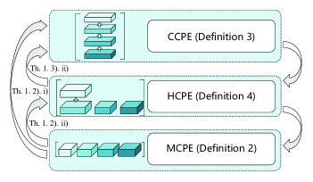
Figure 1: Transformative relationship between the three CPE conditions. The left side of the figure illustrates the synthesis of the conditions, while the right side presents the specific conditions. The arrows denote the derived relationships.

3.1 Three Collectively Persistently Exciting Conditions

In this subsection, we delineate the CPE conditions into three types: cumulative, mosaic, and hybrid, tailored for multi-trajectory sequences. Unlike the traditional PE condition, where each trajectory needs to exhibit sufficient excitation and satisfy identifiable conditions, our approach shifts focus to the collective impact. The three distinct matrix structures afford greater flexibility for trajectories of varying lengths, thereby catering to a wide array of problem types.

Before proceeding, let $\{z_{i}^{[k,k+T_{i}]}\}_{i=1}^{p}$ represent the sequences $z_{1}^{[k,k+T_{1}]},z_{2}^{[k,k+T_{2}]},\ldots,z_{p}^{[k,k+T_{p}]}$, where $z_{i}^{[k,k+T_{i}]}$ denotes the value of the $i$-th signal $z_{i}$ within a specific time interval $[k,k+T_{i}]$, with $T_{i}$ representing a natural number associated with index $i$.

We begin by introducing a mosaic collectively persistently exciting (MCPE) condition for signal sequences of different dimensions, which is shown to be the easiest exciting condition to satisfy in the subsequent discussion (see Theorem 1).

Definition 2

(Collectively Persistently Exciting Condition (Type-I): mosaic). Multiple signals $\{z^{[0,T_{i}-1]}_{i}\}_{i=1}^{p}$ with $z_{i}(k)\in\mathbb{R}^{m}$, $k=0,1,...,{T_{i}-1}$ are mosaic collectively persistently exciting of order $L$ if the matrix

$${H_{L}^{mos}(\{z^{[0,T_{i}-1]}_{i}\}_{i=1}^{p})}$$

$$~~~~~~~~~~~~~~~~~~~={\begin{bmatrix}{{\alpha_{1}}{H_{L}}({z_{1}^{[0,{T_{1}}-1]}})}\ \ldots\ {{\alpha_{p}}{H_{L}}({z_{p}^{[0,{T_{p}}-1]}})}\end{bmatrix}}$$

has full row rank $mL$ for any $\alpha_{i}\neq 0$.

The MCPE condition does not specify the number of dimensions of each signal sequence, i.e., the $T_{i}$ of each signal can be different. Only the sum of all signal lengths is required to satisfy $\sum\limits_{i=1}^{p}{{T_{i}}}\geq mL+p(L-1)$. However, this flexibility results in an unrestricted number of columns in the rank judgment matrix ${H_{L}^{mos}(\{z^{[0,T_{i}-1]}_{i}\}_{i=1}^{p})}$, potentially leading to an excessive number of redundant columns in the matrix. This abundance of columns can significantly increase computational complexity in practical applications such as model predictive control [7, 8, 9].

Therefore, in the following definition, we introduce a cumulative collectively persistently exciting (CCPE) condition for same-dimensional signal sequences. This condition is subsequently confirmed to be the most challenging to satisfy but is the most suitable in terms of computational complexity for application in the design of data-driven control methods.

Definition 3

(Collectively Persistently Exciting Condition (Type-II): cumulative). Multiple signals $\{z^{[0,T_{0}-1]}_{i}\}_{i=1}^{p}$ with $z_{i}(k)\in\mathbb{R}^{m}$, $k=0,1,...,{T_{0}-1}$ are cumulative collectively persistently exciting of order $L$ if the matrix

$${H_{L}^{cum}(\{z^{[0,T_{0}-1]}_{i}\}_{i=1}^{p})}=\sum\limits_{i=1}^{p}{{\alpha_{i}}{H_{L}}({z^{[0,T_{0}-1]}_{i}})}$$

has full row rank $mL$ for any $\alpha_{i}\neq 0$.

The CCPE condition strictly demands that all signal sequences share the same dimension/length, with a minimum requirement of ${T_{0}}\geq(m+1)L-1$. This stringent dimensionality requirement for different signal sequences ensures that the rank-judgment matrix ${H_{L}^{cum}(\{z^{[0,T_{0}-1]}_{i}\}_{i=1}^{p})}$ can be confined to a relatively smaller size, specifically, $mL\times{(T_{0}-L+1)}$ dimensions. Consequently, when it comes to computations using rank judgment matrices, the CCPE condition can better restrict the complexity of the matrices compared to the MCPE condition. This restraint effectively serves the purpose of reducing computational costs.

Next, we introduce a hybrid collectively persistently exciting (HCPE) condition for partially same-dimensional signal sequences. This condition employs a rank judgment matrix that combines the matrix structures from both the CCPE condition and the MCPE condition, leveraging the advantages and mitigating the disadvantages of each.

Definition 4

(Collectively Persistently Exciting Condition (Type-III): hybrid). Multiple signals $\{z^{[0,T_{0}-1]}_{i}\}_{i=1}^{\bar{p}}$ and $\{z^{[0,T_{i}-1]}_{i}\}_{i=\bar{p}+1}^{p}$ with $z_{i}(k)\in\mathbb{R}^{m}$, $k=0,1,...,{T_{i}-1}$ are hybrid collectively persistently exciting of order $L$ if the matrix

$${H_{L}^{hyb}(\{z^{[0,T_{i}-1]}_{i}\}_{i=1}^{p})}$$

$$~~~~~~={\begin{bmatrix}{H_{L}^{cum}(\{z^{[0,T_{0}-1]}_{i}\}_{i=1}^{\bar{p}})}&{H_{L}^{mos}(\{z^{[0,T_{i}-1]}_{i}\}_{i=\bar{p}+1}^{p})}\end{bmatrix}}$$

has full row rank $mL$ for any $\alpha_{i}\neq 0$.

The HCPE condition requires the first $\bar{p}$ signal sequences (which can be any $\bar{p}$ sequences, without loss of generality, and are taken here as the first $\bar{p}$) to be of the same dimension/length, with $T_{0}+\sum\limits_{i=\bar{p}}^{p}{{T_{i}}}\geq mL+(p-\bar{p}+1)(L-1)$.

It is important to note that none of the three CPE conditions require each signal sequence to be persistently exciting. Rather, they allow for insufficient information sequences but mandate that the overall behavior demonstrates a persistently exciting-like performance, which is physically achievable. In Section 4, we propose experimental methods to synthesize the three CPE conditions in cases where each signal segment is not persistently exciting.

Remark 1

The CPE condition proposed in [27] shares similarities with the first type introduced in this paper, the MCPE condition, as both combine Hankel matrices in a side-by-side fashion. However, the MCPE condition distinguishes itself by incorporating weight factors, $\alpha_{i}$, which allows it to perform better when handling data with significant order-of-magnitude differences. Additionally, a careful selection of the weighting factors can enhance both performance and computational efficiency when employing data-driven methods, as demonstrated in the examples in Section 6.1. Notably, despite the introduction of weight factors, the difficulty of synthesis remains unchanged. This is attributed to the fact that for any $\alpha_{i}\neq 0$, the rank of the matrix ${H_{L}^{mos}(\{z^{[0,T_{i}-1]}_{i}\}_{i=1}^{p})}$ remains the same as when $\alpha_{i}=1$.

3.2 Transformation Relations and Rank Conditions of CPE Conditions

In the following result, we analyze the transformation relations between the three CPE conditions. The result reflects the difficulty of realizing the three conditions, and provides some theoretical basis for the selection of the three conditions in practical identification and control problems.

Theorem 1

For multiple signals $\{z^{[0,T_{i}-1]}_{i}\}_{i=1}^{p}$ with $z_{i}(k)\in\mathbb{R}^{m}$, $k=0,1,...,{T_{i}-1}$, the following transformations hold:

• If $\{z_{i}^{[0,{T_{i}-1}]}\}_{i=1}^{p}$ are CCPE $\Longrightarrow$ $\{z_{i}^{[0,{T_{i}-1}]}\}_{i=1}^{p}$ are also MCPE and HCPE;

• If $\{z_{i}^{[0,{T_{i}-1}]}\}_{i=1}^{p}$ are MCPE and satisfy

  • $T_{0}=T_{1}=...=T_{p}$, $\text{im}\,{{H_{L}^{mos}(\{z^{[0,T_{i}-1]}_{i}\}_{i=1}^{p})}^{T}}\cap\text{leftker}\,{\textbf{1}_{p}}\otimes{I_{{T_{0}}-L+1}}=\{0\}$ $\Longrightarrow$ $\{z_{i}^{[0,{T_{i}-1}]}\}_{i=1}^{p}$ are also CCPE;

  • $T_{0}=T_{1}=...=T_{\bar{p}}$, $\text{im}\,{{H_{L}^{mos}(\{z^{[0,T_{i}-1]}_{i}\}_{i=1}^{\bar{p}})}^{T}}\cap\text{leftker}\,{\begin{bmatrix}{{\textbf{1}_{\bar{p}}}}&{{0_{\bar{p}\times(p-\bar{p})}}}\\ {{0_{p-\bar{p}}}}&{{I_{p-\bar{p}}}}\end{bmatrix}}\otimes{I_{{T_{0}}-L+1}}=\{0\}$ $\Longrightarrow$ $\{z_{i}^{[0,{T_{i}-1}]}\}_{i=1}^{p}$ are also HCPE;

• If $\{z_{i}^{[0,{T_{i}-1}]}\}_{i=1}^{p}$ are HCPE,

  • $\{z_{i}^{[0,{T_{i}-1}]}\}_{i=1}^{p}$ are also MCPE;

  • $T_{0}=T_{\bar{p}+1}=...=T_{p}$, $\text{im}\,{{H_{L}^{hyb}(\{z^{[0,T_{i}-1]}_{i}\}_{i=1}^{p})}^{T}}\cap\text{leftker}\,{\textbf{1}_{\bar{p}+1}}\otimes{I_{{T_{0}}-L+1}}=\{0\}$ $\Longrightarrow$ $\{z_{i}^{[0,{T_{i}-1}]}\}_{i=1}^{p}$ are also CCPE.

Proof: See the Appendix. $\blacksquare$

Theorem 1 demonstrates that the MCPE condition is the most straightforward to achieve, followed by the HCPE condition, with the CCPE condition being the most difficult. A significant finding is that satisfying both the CCPE and HCPE conditions results in fulfilling the MCPE condition. Fig. 1 illustrates the transformation relationship among the three conditions.

In the following lemma, we establish the rank condition under three CPE conditions, corresponding to the rank condition (2). This lemma is pivotal in obtaining the accuracy of LS identifier (see Theorem 3) and in extending Willems’ fundamental lemma (see Lemma 2).

Lemma 1

Assuming $\{u_{i}^{[0,{T_{i}-1}]},x_{i}^{[0,{T_{i}-1}]}\}_{i=1}^{p}$ constitutes the $p$-segment input-state trajectory of the system (1).

• If $T_{0}=T_{1}=T_{2}=...=T_{p}$ and $\{u_{i}^{[0,{T_{0}-1}]}\}_{i=1}^{p}$ are CCPE of order $L+n$, then

  $$\text{rank}\begin{bmatrix}{H_{1}^{cum}(\{{x_{i}^{[0,{T_{i}-L}]}\}_{i=1}^{p}})}\\ {H_{L}^{cum}(\{{u_{i}^{[0,{T_{i}-1}]}\}_{i=1}^{p}})}\end{bmatrix}=n+mL.$$

• If $\{u_{i}^{[0,{T_{i}-1}]}\}_{i=1}^{p}$ are MCPE of order $L+n$, then

  $$\text{rank}\begin{bmatrix}{H_{1}^{mos}(\{{x_{i}^{[0,{T_{i}-L}]}\}_{i=1}^{p}})}\\ {H_{L}^{mos}(\{{u_{i}^{[0,{T_{i}-1}]}\}_{i=1}^{p}})}\end{bmatrix}=n+mL.$$

• If $T_{0}=T_{1}=T_{2}=...=T_{\bar{p}}$ and $\{u_{i}^{[0,{T_{i}-1}]}\}_{i=1}^{p}$ are HCPE of order $L+n$, then

  $$\text{rank}\begin{bmatrix}{H_{1}^{hyb}(\{{x_{i}^{[0,{T_{i}-L}]}\}_{i=1}^{p}})}\\ {H_{L}^{hyb}(\{{u_{i}^{[0,{T_{i}-1}]}\}_{i=1}^{p}})}\end{bmatrix}=n+mL.$$

Proof: We begin by demonstrating that

$$\text{rank}\,\begin{bmatrix}{H_{1}^{cum}(\{{x_{i}^{[0,{T_{i}-L}]}\}_{i=1}^{p}})}\\ {H_{L}^{cum}(\{{u_{i}^{[0,{T_{i}-1}]}\}_{i=1}^{p}})}\end{bmatrix}=n+mL,$$

i.e., $\begin{bmatrix}{H_{1}^{cum}(\{{x_{i}^{[0,{T_{i}-L}]}\}_{i=1}^{p}})}\\ {H_{L}^{cum}(\{{u_{i}^{[0,{T_{i}-1}]}\}_{i=1}^{p}})}\end{bmatrix}$ achieves full row rank when $\{u_{i}^{[0,T_{i}-1]}\}_{i=1}^{p}$ is CCPE.

Let $[r_{x}\ r_{u}]\in\text{leftker}\left[{\begin{array}[]{*{20}{c}}{H_{1}^{cum}(\{{x_{i}^{[0,{T_{i}-L}]}\}_{i=1}^{p}})}\\ {H_{L}^{cum}(\{{u_{i}^{[0,{T_{i}-1}]}\}_{i=1}^{p}})}\end{array}}\right]$, where $r_{x}^{T}\in\mathbb{R}^{n}$, $r_{u}^{T}\in\mathbb{R}^{mL}$. In the context of system (1), we konw that

$$\begin{bmatrix}{H_{1}^{cum}(\{{x_{i}^{[1,{T_{i}-L-n+1}]}\}_{i=1}^{p}})}\\ {H_{L}^{cum}(\{{u_{i}^{[1,{T_{i}-n}]}\}_{i=1}^{p}})}\end{bmatrix}=$$

$$\begin{bmatrix}{\begin{bmatrix}A&B\end{bmatrix}}&{{0_{n\times m(n+L-1)}}}\\ {{0_{mL\times(n+m)}}}&{\begin{bmatrix}I_{mL}&{{0}}\end{bmatrix}}\end{bmatrix}\begin{bmatrix}{H_{1}^{cum}(\{{x_{i}^{[0,{T_{i}-L-n}]}\}_{i=1}^{p}})}\\ {H_{L+n}^{cum}(\{{u_{i}^{[0,{T_{i}-1}]}\}_{i=1}^{p}})}\end{bmatrix}$$ (5)

$\vdots$

$$\begin{bmatrix}{H_{1}^{cum}(\{{x_{i}^{[n,{T_{i}-L}]}\}_{i=1}^{p}})}\\ {H_{L}^{cum}(\{{u_{i}^{[n,{T_{i}-1}]}\}_{i=1}^{p}})}\end{bmatrix}=$$

$$\begin{bmatrix}{\begin{bmatrix}{{A^{n}}}&{{A^{n-1}}B}&\cdots&B\end{bmatrix}}&{{0}}\\ {{0_{mL\times n(1+m)}}}&I_{mL}\end{bmatrix}\begin{bmatrix}{H_{1}^{cum}(\{{x_{i}^{[0,{T_{i}-L-n}]}\}_{i=1}^{p}})}\\ {H_{L+n}^{cum}(\{{u_{i}^{[0,{T_{i}-1}]}\}_{i=1}^{p}})}\end{bmatrix}.$$

Since $[r_{x}\ r_{u}]$ also resides in the left kernel of the matrices on the left side of the above equations, a simultaneous left-multiplication of all equations by $[r_{x}\ r_{u}]$ yields

$$R_{x}^{u}\begin{bmatrix}{H_{1}^{cum}(\{{x_{i}^{[0,{T_{i}-L-n}]}\}_{i=1}^{p}})}\\ {H_{L+n}^{cum}(\{{u_{i}^{[0,{T_{i}-1}]}\}_{i=1}^{p}})}\end{bmatrix}={0_{(n+1)\times({T_{i}}-L-n+1)}},$$

where $R_{x}^{u}=\begin{bmatrix}{{r_{x}}}&{{r_{u}}}&{}&{}&{}\\ {{r_{x}}A}&{{r_{x}}B}&{{r_{u}}}&{}&{}\\ \vdots&\ddots&\ddots&\ddots&{}\\ {{r_{x}}{A^{n}}}&{{r_{x}}{A^{n-1}}B}&\cdots&{{r_{x}}B}&{{r_{u}}}\end{bmatrix}$.

Through CCPE condition, one obtains $\text{rank}\,{H_{L+n}^{cum}(\{{u_{i}^{[0,{T_{i}-1}]}\}_{i=1}^{p}})}=m(n+L)$. There must have $\text{dim}(\text{leftker}\begin{bmatrix}{H_{1}^{cum}(\{{x_{i}^{[0,{T_{i}-L-n}]}\}_{i=1}^{p}})}\\ {H_{L+n}^{cum}(\{{u_{i}^{[0,{T_{i}-1}]}\}_{i=1}^{p}})}\end{bmatrix})\leq n$, thus $\text{rank}(R_{x}^{u})\leq n$. Since $R_{x}^{u}$ is a lower triangular block matrix with $n+1$ rows, it follows that at least one of these rows causes $R_{x}^{u}$ to drop rank. Consequently, $r_{u}$ and $r_{x}B$ must both be $0$ vectors. At this point, there are two cases for letting $R_{x}^{u}$ unrank to $n$.

1. There exists a nonzero constant $\tau_{0}$ such that $\tau_{0}r_{x}=r_{x}A$. Then we have $r_{x}AB=\tau_{0}r_{x}B=0$, and further recursion yields $r_{x}A^{n-1}B=r_{x}A^{n-2}B\cdots=r_{x}B=0$. The reachability of $(A,B)$ ensures that $r_{x}=0$.

2. letting $r_{x}A^{j}B=0$, $j=1,2,..,n-1$ and there exists a nonzero constant $\tau_{j}$ such that $\tau_{j}r_{x}A^{j}=r_{x}A^{j+1}$, in which case the same result is obtained with $r_{x}A^{n-1}B=r_{x}A^{n-2}B\cdots=r_{x}B=0$, and thus $r_{x}=0$.

In summary, $\text{rank}(R_{x}^{u})\leq n$ implies that $r_{x}=r_{u}=0$, and thus the matirx $\begin{bmatrix}{H_{1}^{cum}(\{{x_{i}^{[0,{T_{i}-L}]}\}_{i=1}^{p}})}\\ {H_{L}^{cum}(\{{u_{i}^{[0,{T_{i}-1}]}\}_{i=1}^{p}})}\end{bmatrix}$ has full row rank.

Similarly, employing a comparable approach, we can establish that $\begin{bmatrix}{H_{1}^{mos}(\{{x_{i}^{[0,{T_{i}-L}]}\}_{i=1}^{p}})}\\ {H_{L}^{mos}(\{{u_{i}^{[0,{T_{i}-1}]}\}_{i=1}^{p}})}\end{bmatrix}$ or $\begin{bmatrix}{H_{1}^{hyb}(\{{x_{i}^{[0,{T_{i}-L}]}\}_{i=1}^{p}})}\\ {H_{L}^{hyb}(\{{u_{i}^{[0,{T_{i}-1}]}\}_{i=1}^{p}})}\end{bmatrix}$ achieves full row rank when $\{u_{i}^{[0,{T_{i}-1}]}\}_{i=1}^{p}$ is MCPE or HCPE of order $L+n$. We will not reiterate this here. $\blacksquare$

4 Experimental Design for CPE Conditions

In this section, we propose the experimental design approach to fulfill the three CPE conditions. The design process is guided by two requirements: 1). Each signal must be non-persistently exciting. 2). The design process can be applicable both online and offline. The design idea of the experiment will be reflected in the proof of Theorem 2.

Signal design for the MCPE condition:

Consider multiple signals $\{z^{[0,T_{i}-1]}_{i}\}_{i=1}^{p}$, where $z_{i}(k)\in\mathbb{R}^{m}$ for $k=0,1,...,{T_{i}-1}$. Without loss of generality, assume that $L\leq T_{1}\leq T_{2}\leq...\leq T_{p}<(m+1)L$. Define $\Delta_{1}=L-1$, $\Delta_{i}=L-1-\text{mod}(\sum^{i-1}_{j=1}(T_{j}-L+1),L)$ for $i>1$, $T_{1}^{s}=0$, and $T_{i}^{s}=\sum^{i-1}_{j=1}(T_{j}-L+1)$ for $i>1$.

Construction of $z_{i}(0),z_{1}(1),\ldots,z_{i}(L-1)$ for $i=1,\ldots,p$:

• For $i=1$:

  Select $z_{i}^{[0,L-2]}$ arbitrarily, and set $\text{rank}\ z_{i}(L-1)=1$.

• For $i>1$:

  Select $z_{i}^{[0,\Delta_{i}-1]}$ arbitrarily for $\Delta_{i}>1$, and choose $z_{i}(\Delta_{i})$ as follows:

  $\begin{cases}z_{i}(\Delta_{i})\notin\text{im}\ [z_{1}\left(\Delta_{1}\right)\ \cdots\ z_{i-1}(\Delta_{i-1})],&\\ \ \ \ \ \ \ \text{if}\ T_{i-1}\geqslant\Delta_{i-1}+L\ \text{and}\ T_{i}^{s}<\left(m+1\right)L-1,&\\ z_{i}\left(\Delta_{i}\right)\in\text{im}\ z_{i-1}\left(\Delta_{i-1}\right),\ \ \ \text{otherwise}.&\end{cases}$

  Then, set $\ z^{[\Delta_{i}+1,L-1]}_{i}=0$ for $\Delta_{i}<L-1$.

Construction of $z_{i}(L),z_{i}(L+1),\ldots,z_{i}(T_{i}-1)$ for $i=1,\ldots,p$:

• For $k<T_{i}$ and $T_{i}^{s}+k\in\{2L-1,3L-1,\ldots,(m+1)L-1\}$:

  Select $z_{i}(k)$ as follows:

  $\begin{cases}z_{i}(k)\notin\text{im}\ [z_{1}\left(\Delta_{1}\right)\cdots z_{p}(\Delta_{p})\ \bar{z}_{1}\cdots\bar{z}_{p}],&\text{if}\ T_{i}-k\geqslant L,\\ z_{i}\left(k\right)\in\text{im}\ z_{i+1}\left(\Delta_{i+1}\right),&\text{otherwise},\end{cases}$ where $\bar{z}_{i}=[z_{i}(L-1)\ z_{i}(2L-1)\cdots]$.

• For $k<T_{i}$ and $T_{i}^{s}+k\notin\{2L-1,3L-1,\ldots,(m+1)L-1\}$:

  Set $z_{i}(k)=0$.

Signal design for the CCPE condition:

Consider multiple signals $\{z^{[0,T_{0}-1]}_{i}\}_{i=1}^{p}$, where $z_{i}(k)\in\mathbb{R}^{m}$ for $k=0,1,...,{T_{0}-1}$. Define $Z_{i}^{j}=\left[z_{i}\begin{matrix}\left(j\right)&z_{i}\left(j+L\right)&\cdots&z_{i}(j+\left(m-1)L\right)\end{matrix}\right]$.

Construction of $z_{i}(0),...,z_{i}(mL-1)$ for $i=1,\ldots,p$:

• Choose $z_{i}(k)$ such that $\text{rank}\ \sum^{p}_{i=1}\alpha_{i}z_{i}\left(k\right)=1$ for $k\in\{L-1,2L-1,\ldots,mL-1\}$, and $\sum^{p}_{i=1}\alpha_{i}z_{i}\left(k\right)=0$ otherwise.

• Ensure that

  $$\sum^{p}_{i=1}\alpha_{i}\left[z_{i}\begin{matrix}\left(L-1\right)&z_{i}\left(2L-1\right)&\cdots&z_{i}\left(mL-1\right)\end{matrix}\right]$$

  has full rank.

• Ensure $\text{rank}\ Z_{i}^{0}=m$ for $i=1,\ldots,p$.

Construction of $z_{i}(k),k>mL-1$ for $i=1,\ldots,p$:

• Design $z_{i}\left(k\right)$ as

  $$z_{i}\left(k\right)=Z^{(k-mL+1)}_{i}({Z^{0}_{i})}^{-1}z_{i}\left(mL-1\right).$$ (6)

Signal design for the HCPE condition:

Consider multiple signals $\{z^{[0,T_{0}-1]}_{i}\}_{i=1}^{\bar{p}}$ and $\{z^{[0,T_{i}-1]}_{i}\}_{i=\bar{p}+1}^{p}$, where $z_{i}(k)\in\mathbb{R}^{m}$, $k=0,1,\ldots,{T_{i}-1}$. Without loss of generality, assume that $L\leq\bar{p}+1\leq\bar{p}+2\leq...\leq p<(m+1)L$.

Construction of $z_{i}(0),\ldots,z_{i}(T_{0}-1)$ for $i=1,\ldots,\bar{p}:$

• If $T_{0}\geqslant(m+1)L$:

  Use the CCPE signal design method.

• If $T_{0}<(m+1)L$:

  Choose $z_{i}(k)$ such that $\text{rank}\ \sum^{\bar{p}}_{i=1}\alpha_{i}z_{i}\left(k\right)=1$ for $k\in\{L-1,2L-1,\ldots,mL-1\}$, and $\sum^{\bar{p}}_{i=1}\alpha_{i}z_{i}\left(k\right)=0$ otherwise. Ensure that

  $$\sum^{\bar{p}}_{i=1}\alpha_{i}\left[z_{i}\begin{matrix}\left(L-1\right)&z_{i}\left(2L-1\right)&\cdots\end{matrix}\right]$$

  has full column rank.

Construction of $z_{i}(0),\ldots,z_{i}(T_{i}-1)$ for $i=\bar{p}+1,\ldots,p$:

• Let $\sum^{\bar{p}}_{i=1}\alpha_{i}z_{i}$ represent the initial signal, with $\{z_{i}\}_{i=\bar{p}+1}^{p}$ serving as the subsequent signals. Employ the MCPE signal design method to construct $z_{i}(0),\ldots,z_{i}(T_{i}-1)$ for $i=\bar{p}+1,\ldots,p$.

Theorem 2

For multiple signals $\{z^{[0,T_{i}-1]}_{i}\}_{i=1}^{p}$, where $z_{i}(k)\in\mathbb{R}^{m}$ for $k=0,1,\ldots,{T_{i}-1}$.

• Using the MCPE design method, the signal length required to satisfy $\text{rank}\ {H_{L}^{mos}(\{z^{[0,T_{i}-1]}_{i}\}_{i=1}^{p})}=mL$ is $\sum\limits_{i=1}^{p}{{T_{i}}}\geq mL+p(L-1)$.

• Using the CCPE design method, the signal length required to satisfy $\text{rank}\ {H_{L}^{cum}(\{z^{[0,T_{0}-1]}_{i}\}_{i=1}^{p})}=mL$ is ${T_{0}}\geq(m+1)L-1$.

• Using the HCPE design method, the signal length required to satisfy $\text{rank}\ {H_{L}^{hyb}(\{z^{[0,T_{i}-1]}_{i}\}_{i=1}^{p})}=mL$ is $T_{0}+\sum\limits_{i=\bar{p}}^{p}{{T_{i}}}\geq mL+(p-\bar{p}+1)(L-1)$.

Additionally, all three design methods ensure that each sub-signal is non-persistently exciting, i.e., $\text{rank}\ {H_{L}}({z_{i}^{[0,T_{i}-1]}})<mL$.

Proof: 1). For the MCPE condition, the design ensures that the matrix ${H_{L}^{mos}(\{z^{[0,T_{i}-1]}_{i}\}_{i=1}^{p})}$ takes the following form:

Each group of $L$ columns forms an approximately upper triangular structure, with the diagonal elements of the first $m$ submatrices being linearly independent. To construct the desired matrix using $p$ signals, it is necessary to identify which of the first $L$ values of each signal appears as diagonal elements in the submatrices, i.e., $z_{i}(\Delta(i))$. If $T_{i-1}\geq\Delta_{i-1}+L$, then a submatrix spans from $z_{i-1}(\Delta(i-1))$ to $z_{i}(\Delta(i))$, and $z_{i}(\Delta(i))$ must be designed such that $z_{i}(\Delta_{i})\notin\text{im}\ [z_{1}(\Delta_{1})\cdots z_{i-1}(\Delta_{i-1})]$. Otherwise, the submatrix is not spanned, and $z_{i}(\Delta(i))$ is chosen as $z_{i}(\Delta_{i})\in\text{im}\ z_{i-1}(\Delta_{i-1})$.

For $k>L-1$, if $z_{i}(k)$ corresponds to the start of the diagonal of a submatrix, i.e., $T_{i}^{s}+k\in\{2L-1,3L-1,\ldots,(m+1)L-1\}$, it is necessary to verify whether $z_{i}$ can still form $L$ columns. If feasible, $z_{i}(k)$ is designed to remain linearly independent from the existing diagonal elements, i.e., $z_{i}(k)\notin\text{im}\ [z_{1}\left(\Delta_{1}\right)\cdots z_{p}(\Delta_{p})\ \bar{z}_{1}\cdots\bar{z}_{p}]$. If this is not feasible, then $z_{i}(k)\in\text{im}\ z_{i+1}(\Delta_{i+1})$.

The remaining design choices ensure that the $p$ signals collectively construct the desired matrix while satisfying the length constraint $T_{i}<(m+1)L$ if $p>1$. Therefore,

$$\text{rank}\ {H_{L}}({z_{i}^{[0,T_{i}-1]}})<mL.$$

2). Since $\text{rank}\ \sum^{p}_{i=1}\alpha_{i}z_{i}\left(k\right)=1$ for $k\in\{L-1,2L-1,....,mL-1\}$, and $\sum^{p}_{i=1}\alpha_{i}z_{i}\left(k\right)=0$ otherwise, we have

$$\text{rank}\ {H_{L}^{cum}(\{z^{[kL,(k+2)(L-1)]}_{i}\}_{i=1}^{p})}=L$$

for all $k\text{}\in\left\{0,1,...,m-1\right\}$. At this point, ${H_{L}^{cum}(\{z^{[kL,(k+2)(L-1)]}_{i}\}_{i=1}^{p})}$ takes the form of a lower triangular matrix with nonzero diagonal elements, i.e.,

$${H_{L}^{cum}(\{z^{[kL,(k+2)(L-1)]}_{i}\}_{i=1}^{p})}$$

$$=\begin{bmatrix}0&&&z^{cum}_{(k+1)(L-1)}\\ &&\iddots&z^{cum}_{k(L-1)+L}\\ &z^{cum}_{(k+1)(L-1)}&\iddots&\vdots\\ z^{cum}_{(k+1)(L-1)}&z^{cum}_{k(L-1)+L}&\cdots&z^{cum}_{(k+2)(L-1)}\end{bmatrix},$$

where $z^{cum}_{k}=\sum^{p}_{i=1}\alpha_{i}z_{i}\left(k\right)$.

Since $\sum^{p}_{i=1}\alpha_{i}\left[z_{i}\begin{matrix}\left(L-1\right)&z_{i}\left(2L-1\right)&\cdots&z_{i}\left(mL-1\right)\end{matrix}\right]$ has full rank, the choice of $z_{i}(k)$, $k\notin\{L-1,2L-1,....,mL-1\}$ at each time step increases the rank of the cumulative Hankel matrix ${H_{L}^{cum}(\{z^{[0,T_{0}-1]}_{i}\}_{i=1}^{p})}$ until it becomes full rank at $T_{0}=(m+1)L$.

Next, we demonstrate that designing $z_{i}(k)$ for $k>mL-1$ according to the proposed approach ensures that each sub-Hankel matrix does not satisfy $mL$-order persistently exciting. Specifically, since $Z_{i}^{0}$ is full rank for $i=1,\dots,p$, there always exists a design law as described in (6). Consequently, we have

$$z^{[k,k+L-1]}_{i}\in\text{im}\left[\begin{matrix}Z^{k-mL+1}_{i}\\ Z^{k-mL+2}_{i}\\ \vdots\\ Z^{k-(m-1)L}_{i}\end{matrix}\right],k\geqslant mL-1$$

for all $i\in\{1,\dots,p\}$. This result implies that the rank of the Hankel matrix $H_{L}(z_{i}^{[0,T_{0}-1]})$ cannot increase beyond the $mL$-th column. Therefore,

$$\text{rank}\ {H_{L}}({z_{i}^{[0,{T_{0}}-1]}})<mL.$$

3). Building upon the proof procedures for signal design under the MCPE and CCPE conditions, the HCPE condition can be similarly achieved. Specifically, the matrix $H_{L}^{hyb}(\{z^{[0,T_{i}-1]}i\}{i=1}^{p})$ attains full row rank if $T_{0}+\sum_{j=\bar{p}+1}^{p}T_{j}\geq(m+1)L$, and each signal exhibits non-$mL$-order persistently exciting. $\blacksquare$

Remark 2

According to Theorem 2, we find that all three conditions can be satisfied within the minimum number of time steps. Specifically, if we fix ${H_{L}^{mos}(\{z^{[0,T_{i}-1]}_{i}\}_{i=1}^{p})}$, ${H_{L}^{cum}(\{z^{[0,T_{0}-1]}_{i}\}_{i=1}^{p})}$, and ${H_{L}^{hyb}(\{z^{[0,T_{i}-1]}_{i}\}_{i=1}^{p})}$ as standard square matrices, the experimental design method outlined in Section 4 can achieve the required conditions. In this scenario, the eigenvalues of the three composite matrices depend solely on the elements along the diagonal of each $L$ column. Furthermore, we note that the experimental design methods for all three conditions do not require knowledge of future information, allowing them to be implemented either offline or online. This enables real-time adjustment of control signals based on system state constraints while satisfying design requirements, thereby preventing extreme state divergence.

5 Applications of CPE Conditions

In this section, we validate the effectiveness of the three conditions through least squares identification and Williams’ fundamental lemma. First, we present convergence results for the three conditions under LS identification, focusing on the impact of the singular values of the three synthetic matrices on the convergence error. Subsequently, we derive extended results of Willems’ fundamental lemma under the three CPE conditions.

5.1 Least-squares identification under CPE conditions

Consider a group of LTI systems with $N$ agents, the dynamics of each agent are given by

$$x_{i}(k+1)=Ax_{i}(k)+Bu_{i}(k)+w_{i}(k),\ i=1,2,...,N$$ (7)

where ${x_{i}(k)}\in{\mathbb{R}^{n}}$, ${u_{i}(k)}\in{\mathbb{R}^{m}}$, and $w_{i}(k)\in{\mathbb{R}^{n}}$ represent the system state, input and process noise, respectively. It is assumed that the process noises is i.i.d. Gaussian, i.e., $w(k)\sim\mathcal{N}(0,\sigma_{w}^{2}I)$.

For each agent, the input/state data is organized as

$$U_{i}=\left[\begin{matrix}u_{i}\left(0\right)&u_{i}\left(1\right)&\cdots&u_{i}\left(T_{i}-1\right)\end{matrix}\right],$$

$$X_{i}^{-}=\left[\begin{matrix}x_{i}\left(0\right)&x_{i}\left(1\right)&\cdots&x_{i}\left(T_{i}-1\right)\end{matrix}\right],$$

$$X_{i}^{+}=\left[\begin{matrix}x_{i}\left(1\right)&x_{i}\left(2\right)&\cdots&x_{i}\left(T_{i}\right)\end{matrix}\right],$$

$$X_{i}^{n}=\left[\begin{matrix}x_{i}\left(0\right)&x_{i}\left(1\right)&\cdots&x_{i}\left(T_{i}-1-n\right)\end{matrix}\right],$$

and the process noise data as

$$W_{i}=\left[\begin{matrix}w_{i}\left(0\right)&w_{i}\left(1\right)&\cdots&w_{i}\left(T_{i}-1\right)\end{matrix}\right],$$

$$W_{i}^{n}=\left[\begin{matrix}w_{i}\left(0\right)&w_{i}\left(1\right)&\cdots&w_{i}\left(T_{i}-1-n\right)\end{matrix}\right].$$

The data combinations in Definitions 2-4 can be freely selected according to the length of the input data of the $N$ agents. For example, consider the CCPE condition. If $T_{1}=T_{2}=...=T_{N}=T_{0}$, $N$ sets of input data can be combined as

$$H^{cum}_{L}\left(\{U_{i}\}^{N}_{i=1}\right)=\sum\limits^{N}_{i=1}{{\alpha_{i}}{H_{L}}(U_{i})}.$$

From the system dynamics (7), we obtain

$$H^{cum}_{1}\left(\{X^{+}_{i}\}^{N}_{i=1}\right)$$

$$=\begin{bmatrix}A&B\end{bmatrix}\left[\begin{matrix}H^{cum}_{1}\left(\{X^{-}_{i}\}^{N}_{i=1}\right)\\ H^{cum}_{1}\left(\{U_{i}\}^{N}_{i=1}\right)\end{matrix}\right]+H^{cum}_{1}\left(\{W_{i}\}^{N}_{i=1}\right).$$ (8)

Define $G=\begin{bmatrix}A&B\end{bmatrix}$. The least squares problem is formulated as

$$\text{}\min_{G}\left\|H^{cum}_{1}\left(\{X^{+}_{i}\}^{N}_{i=1}\right)-G\left[\begin{matrix}H^{cum}_{1}\left(\{X^{-}_{i}\}^{N}_{i=1}\right)\\ H^{cum}_{1}\left(\{U_{i}\}^{N}_{i=1}\right)\end{matrix}\right]\right\|$$

The solution, unique due to Lemma 1, is given by

$$\hat{G}={H^{cum}_{1}(\{X_{i}^{+}\}^{N}_{i=1})}{\begin{bmatrix}{H^{cum}_{1}(\{X_{i}^{-}\}^{N}_{i=1})}\\ {H^{cum}_{1}(\{U_{i}\}^{N}_{i=1})}\end{bmatrix}^{{\dagger}}}.$$ (9)

Subsequently, we abbreviate ${H^{cum}_{n+1}(\{U_{i}\}^{N}_{i=1})}$, ${H^{mos}_{n+1}(\{U_{i}\}^{N}_{i=1})}$, and ${H^{hyb}_{n+1}(\{U_{i}\}^{N}_{i=1})}$ as ${U^{cum}_{n+1}}$, ${U^{mos}_{n+1}}$, and ${U^{hyb}_{n+1}}$, respectively.

Theorem 3

Using the LS identifiers for the MCPE, CCPE, and HCPE conditions, respectively, the estimation error is bounded as follows:

1). $\left\|\hat{G}-G\right\|_{2}\leq\frac{\sigma_{w}{\sqrt{n+1}}\left(\sqrt{n}+\sqrt{T_{0}}\right)\sum^{N}_{i=1}\alpha_{i}}{\rho^{cum}_{0}\underline{\sigma}({U^{cum}_{n+1}})-\rho^{cum}_{1}\sigma_{w}\sqrt{n}\left(\sqrt{n}+\sqrt{T_{0}-n}\right)\sum^{N}_{i=1}\alpha_{i}}$ if inputs $\{U_{i}\}_{i=1}^{p}$ are CCPE of order $n+1$, where $\rho^{cum}_{0},\rho^{cum}_{1}$ are defined in (13).

2). $\left\|\hat{G}-G\right\|_{2}\leq\frac{\sigma_{w}{\sqrt{n+1}}\sum^{N}_{i=1}\alpha_{i}\left(\sqrt{n}+\sqrt{T_{i}}\right)}{\rho^{mos}_{0}\underline{\sigma}({U^{mos}_{n+1}})-\rho^{mos}_{1}\sigma_{w}\sqrt{n}\sum^{N}_{i=1}\alpha_{i}\left(\sqrt{n}+\sqrt{T_{i}-n}\right)}$ if inputs $\{U_{i}\}_{i=1}^{p}$ are MCPE of order $n+1$, where $\rho^{mos}_{0},\rho^{mos}_{1}$ are defined in (15).

3). $\left\|\hat{G}-G\right\|_{2}\leq\frac{\sigma_{w}{\sqrt{n+1}}\sum^{N}_{i=1}\alpha_{i}\left(\sqrt{n}+\sqrt{T_{i}}\right)}{\rho^{cum}_{0}\underline{\sigma}({U^{hyb}_{n+1}})-\rho^{hyb}_{1}\sigma_{w}\sqrt{n}\sum^{N}_{i=1}\alpha_{i}\left(\sqrt{n}+\sqrt{T_{i}-n}\right)}$ if inputs $\{U_{i}\}_{i=1}^{p}$ are HCPE of order $n+1$, where $\rho^{hyb}_{0},\rho^{hyb}_{1}$ are defined in (16).

Proof: From (5.1) and (9), the estimation error for the CCPE condition is given by

$$\left\|\hat{G}-G\right\|_{2} =\left\|H^{cum}_{1}\left(\{W_{i}\}^{N}_{i=1}\right){\begin{bmatrix}{H^{cum}_{1}(\{X_{i}\}^{N}_{i=1})}\\ {H^{cum}_{1}(\{U_{i}\}^{N}_{i=1})}\end{bmatrix}^{{\dagger}}}\right\|_{2}$$

$$\leq\frac{\overline{\sigma}\left(H^{cum}_{1}\left(\{W_{i}\}^{N}_{i=1}\right)\right)}{\underline{\sigma}\left({\begin{bmatrix}{H^{cum}_{1}(\{X_{i}\}^{N}_{i=1})}\\ {H^{cum}_{1}(\{U_{i}\}^{N}_{i=1})}\end{bmatrix}}\right)}.$$ (10)

Denote ${\underline{\sigma}}^{cum}={\underline{\sigma}\left({\begin{bmatrix}{H^{cum}_{1}(\{X_{i}\}^{N}_{i=1})}\\ {H^{cum}_{1}(\{U_{i}\}^{N}_{i=1})}\end{bmatrix}}\right)}$ and the corresponding left and right singular vectors of ${\underline{\sigma}}^{cum}$ as $\xi^{cum}=\left[\begin{matrix}\xi_{x}^{cum}&\xi_{u}^{cum}\end{matrix}\right]^{T}$ and $\nu^{cum}$, where ${\xi_{x}^{cum}}^{T}\in\mathbb{R}^{n}$, ${\xi_{u}^{cum}}^{T}\in\mathbb{R}^{L}$, and $\nu^{cum}\in\mathbb{R}^{T_{0}}$. We have

$$\left[\begin{matrix}\xi_{x}^{cum}&\xi_{u}^{cum}\end{matrix}\right]{\begin{bmatrix}{H^{cum}_{1}(\{X_{i}\}^{N}_{i=1})}\\ {H^{cum}_{1}(\{U_{i}\}^{N}_{i=1})}\end{bmatrix}}={\underline{\sigma}}^{cum}\nu^{T}.$$ (11)

According to (3.2), (11), and the dynamics (7), we have

$$\Phi_{\xi}^{cum}\begin{bmatrix}{H^{cum}_{1}(\{{X^{n}_{i}\}^{N}_{i=1}})}\\ {U^{cum}_{n+1}}\end{bmatrix}+\Psi_{\xi}^{cum}H^{cum}_{n}\left(\{W_{i}^{1}\}^{N}_{i=1}\right)$$

$$={\underline{\sigma}}^{cum}H_{n+1}\left(v^{\left[0,T_{0}-1\right]}\right),$$ (12)

where

$$\Phi_{\xi}^{cum}=\begin{bmatrix}{{\xi_{x}^{cum}}}&{{\xi_{u}^{cum}}}&{}&{}&{0}\\ {\xi_{x}^{cum}A}&{{\xi_{x}^{cum}}B}&{{\xi_{u}^{cum}}}&{}&{}\\ \vdots&\ddots&\ddots&\ddots&{}\\ {\xi_{x}^{cum}{A^{n}}}&{\xi_{x}^{cum}{A^{n-1}}B}&\cdots&{\xi_{x}^{cum}B}&{{\xi_{u}^{cum}}}\end{bmatrix},$$

$$\Psi_{\xi}^{cum}=\left[\begin{matrix}0&&&0\\ \xi_{x}^{cum}&0&&\\ \xi_{x}^{cum}A&\xi_{x}^{cum}&\ddots&\\ \vdots&\ddots&\ddots&0\\ \xi_{x}^{cum}A^{n-1}&\ldots&\xi_{x}^{cum}A&\xi_{x}^{cum}\end{matrix}\right].$$

Since ${\xi^{cum}}^{T}\xi^{cum}=1$, according to the proof process of Lemma 1, we have $\text{rank}\ \Phi_{\xi}^{cum}=n+1$, therefore ${\underline{\sigma}}(\Phi_{\xi}^{cum})>0\geqslant\rho^{cum}_{0}$ with $\rho^{cum}_{0}>0$. Then (5.1) can be deflated as

$${\underline{\sigma}}(\Phi_{\xi}^{cum})\underline{\sigma}(U^{cum}_{d})\leq{\underline{\sigma}}(\Phi_{\xi}^{cum}){\underline{\sigma}}(\begin{bmatrix}{H^{cum}_{1}(\{{X^{n}_{i}\}^{N}_{i=1}})}\\ {U^{cum}_{n+1}}\end{bmatrix})$$

$$\leq\left\|\Phi_{\xi}^{cum}\begin{bmatrix}{H^{cum}_{1}(\{{X^{n}_{i}\}^{N}_{i=1}})}\\ {U^{cum}_{n+1}}\end{bmatrix}\right\|$$

$$=\left\|{\underline{\sigma}}^{cum}H_{n+1}\left(v^{\left[0,T_{0}-1\right]}\right)-\Psi_{\xi}^{cum}H^{cum}_{n}\left(\{W^{1}_{i}\}^{N}_{i=1}\right)\right\|$$

$$\leq{\underline{\sigma}}^{cum}\left\|H_{n+1}\left(v^{\left[0,T_{0}-1\right]}\right)\right\|+\left\|\Psi_{\xi}^{cum}H^{cum}_{n}\left(\{W^{1}_{i}\}^{N}_{i=1}\right)\right\|.$$

Since $\nu^{T}\nu=1$, we have $\left\|H_{n+1}\left(v^{\left[0,T_{0}-1\right]}\right)\right\|\leq\sqrt{n+1}$. Let

$${\underline{\sigma}}(\Phi_{\xi}^{cum})=\rho^{cum}_{0},\rho^{cum}_{0}>0,\left\|\Psi_{\xi}^{cum}\right\|\leq\rho^{cum}_{1}.$$ (13)

Therefore,

$${\underline{\sigma}}^{cum}\geqslant\frac{\rho^{cum}_{0}\underline{\sigma}(U^{cum}_{n+1})-\rho^{cum}_{1}\left\|H^{cum}_{n}\left(\{W^{1}_{i}\}^{N}_{i=1}\right)\right\|}{\sqrt{n+1}}.$$

Combining the above with (5.1) yields

$$\left\|\hat{G}-G\right\| \leq\frac{{\sqrt{n+1}}\overline{\sigma}\left(H^{cum}_{1}\left(\{W_{i}\}^{N}_{i=1}\right)\right)}{\rho^{cum}_{0}\underline{\sigma}(U^{cum}_{n+1})-\rho^{cum}_{1}\left\|H^{cum}_{n}\left(\{W^{1}_{i}\}^{N}_{i=1}\right)\right\|}.$$ (14)

According to the theory of random matrices, we have

$$\overline{\sigma}\left(H^{cum}_{1}\left(\{W_{i}\}^{N}_{i=1}\right)\right) \leqslant\sum^{N}_{i=1}\alpha_{i}\overline{\sigma}(W_{i})$$

$$\leq\sigma_{w}\left(\sqrt{n}+\sqrt{T_{0}}\right)\sum^{N}_{i=1}\alpha_{i},$$

$$\left\|H^{cum}_{n}\left(\{W^{1}_{i}\}^{N}_{i=1}\right)\right\| \leq\sigma_{w}\sqrt{n}\left(\sqrt{n}+\sqrt{T_{0}-n}\right)\sum^{N}_{i=1}\alpha_{i}$$

Conclusion 1) can be obtained by substituting these bounds into (14).

Similarly, we can define

$${\underline{\sigma}}(\Phi_{\xi}^{mos})=\rho^{mos}_{0},\rho^{mos}_{0}>0,\left\|\Psi_{\xi}^{mos}\right\|\leq\rho^{mos}_{1}.$$ (15)

$${\underline{\sigma}}(\Phi_{\xi}^{hyb})=\rho^{hyb}_{0},\rho^{hyb}_{0}>0,\left\|\Psi_{\xi}^{hyb}\right\|\leq\rho^{hyb}_{1}.$$ (16)

Furthermore, we have

$$\overline{\sigma}\left(H^{mos}_{1}\left(\{W_{i}\}^{N}_{i=1}\right)\right) \leq\sigma_{w}\sum^{N}_{i=1}\alpha_{i}\left(\sqrt{n}+\sqrt{T_{i}}\right),$$

$$\left\|H^{mos}_{n}\left(\{W^{1}_{i}\}^{N}_{i=1}\right)\right\| \leq\sigma_{w}\sqrt{n}\sum^{N}_{i=1}\alpha_{i}\left(\sqrt{n}+\sqrt{T_{i}-n}\right),$$

$$\overline{\sigma}\left(H^{hyb}_{1}\left(\{W_{i}\}^{N}_{i=1}\right)\right) \leq\sigma_{w}\sum^{N}_{i=1}\alpha_{i}\left(\sqrt{n}+\sqrt{T_{i}}\right),$$

$$\left\|H^{hyb}_{n}\left(\{W^{1}_{i}\}^{N}_{i=1}\right)\right\| \leq\sigma_{w}\sqrt{n}\sum^{N}_{i=1}\alpha_{i}\left(\sqrt{n}+\sqrt{T_{i}-n}\right),$$

The proofs of conclusions 2) and 3) follow a similar process and are omitted here. $\blacksquare$

5.2 Extension of Fundamental Lemma

In this subsection, we delve into the fundamental lemmas under the CPE condition, extending the traditional Willems’ lemma.

For a single-input signal sequence satisfying the PE condition of order $L+n$, (3) always holds. A similar conclusion applies when the signal sequence extends to more than one, as described by the following theorem.

Lemma 2

Assuming $\{u_{i}^{[0,{T_{i}-1}]},x_{i}^{[0,{T_{i}-1}]}\}_{i=1}^{p}$ constitutes the $p$-segment input-state trajectory of the system (1). Then, the following holds.

• If $T_{0}=T_{1}=T_{2}=...=T_{p}$ and $\{u_{i}^{[0,{T_{i}-1}]}\}_{i=1}^{p}$ are CCPE of order $L+n$, then any $L$-long input-state trajectory of system (1) can be expressed as

  $$\begin{bmatrix}{H_{L}^{cum}(\{{x_{i}^{[0,{T_{i}-1}]}\}_{i=1}^{p}})}\\ {H_{L}^{cum}(\{{u_{i}^{[0,{T_{i}-1}]}\}_{i=1}^{p}})}\end{bmatrix}g,$$

  where $g$ is a real vector.

• If $\{u_{i}^{[0,{T_{i}-1}]}\}_{i=1}^{p}$ are MCPE of order $L+n$, then any $L$-long input-state trajectory of system (1) can be expressed as

  $$\begin{bmatrix}{H_{L}^{mos}(\{{x_{i}^{[0,{T_{i}-1}]}\}_{i=1}^{p}})}\\ {H_{L}^{mos}(\{{u_{i}^{[0,{T_{i}-1}]}\}_{i=1}^{p}})}\end{bmatrix}g,$$

  where $g$ is a real vector.

• If $T_{0}=T_{1}=T_{2}=...=T_{\bar{p}}$ and $\{u_{i}^{[0,{T_{i}-1}]}\}_{i=1}^{p}$ are HCPE of order $L+n$, then any $L$-long input-state trajectory of system (1) can be expressed as

  $$\begin{bmatrix}{H_{L}^{hyb}(\{{x_{i}^{[0,{T_{i}-1}]}\}_{i=1}^{p}})}\\ {H_{L}^{hyb}(\{{u_{i}^{[0,{T_{i}-1}]}\}_{i=1}^{p}})}\end{bmatrix}g,$$

  where $g$ is a real vector.

Proof: By the dynamics of system (1), one has

$$\begin{bmatrix}{H_{L}^{cum}(\{{u_{i}^{[0,{T_{0}-1}]}\}_{i=1}^{p}})}\\ {H_{L}^{cum}(\{{x_{i}^{[0,{T_{0}-1}]}\}_{i=1}^{p}})}\end{bmatrix}g$$

$$~~~~~~~~~~~~~~=\begin{bmatrix}I&0\\ \mathcal{T}_{L}&\mathcal{O}_{L}\end{bmatrix}\begin{bmatrix}{H_{L}^{cum}(\{{u_{i}^{[0,{T_{0}-1}]}\}_{i=1}^{p}})}\\ {H_{1}^{cum}(\{{x_{i}^{[0,{T_{0}-L}]}\}_{i=1}^{p}})}\end{bmatrix}g,$$ (17)

where $\mathcal{T}_{L}$ and $\mathcal{O}_{L}$ are defined as

$${{\cal T}_{L}}=\begin{bmatrix}0&0&0&\cdots&0\\ B&0&0&\cdots&0\\ {AB}&B&0&\cdots&0\\ \vdots&\vdots&\vdots&\ddots&\vdots\\ {{A^{L-2}}B}&{{A^{L-2}}B}&{{A^{L-2}}B}&\cdots&0\end{bmatrix}$$

$${{\cal O}_{L}}={\begin{bmatrix}I&{{A^{T}}}&{{{({A^{2}})}^{T}}}&\cdots&{{{({A^{L-1}})}^{T}}}\end{bmatrix}^{T}}.$$

Since $\begin{bmatrix}{H_{L}^{cum}(\{{u_{i}^{[0,{T_{0}-1}]}\}_{i=1}^{p}})}\\ {H_{1}^{cum}(\{{x_{i}^{[0,{T_{0}-L}]}\}_{i=1}^{p}})}\end{bmatrix}$ has full row rank by Lemma 1, all vectors consisting of the initial state $\bar{x}(0)$ and the $L$-long input sequence $\bar{u}^{[0,L-1]}$ of system (1) can be represented by a linear combination of the columns of $\begin{bmatrix}{H_{L}^{cum}(\{{u_{i}^{[0,{T_{0}-1}]}\}_{i=1}^{p}})}\\ {H_{1}^{cum}(\{{x_{i}^{[0,{T_{0}-L}]}\}_{i=1}^{p}})}\end{bmatrix}$, i.e.,

$$\begin{bmatrix}{H_{L}^{cum}(\{{u_{i}^{[0,{T_{0}-1}]}\}_{i=1}^{p}})}\\ {H_{1}^{cum}(\{{x_{i}^{[0,{T_{0}-L}]}\}_{i=1}^{p}})}\end{bmatrix}g=\begin{bmatrix}{{{\bar{u}}^{[0,L-1]}}}\\ {{{\bar{x}}(0)}}\end{bmatrix}.$$

Therefore, (5.2) can be transformed into

$$\begin{bmatrix}{H_{L}^{cum}(\{{u_{i}^{[0,{T_{0}-1}]}\}_{i=1}^{p}})}\\ {H_{L}^{cum}(\{{x_{i}^{[0,{T_{0}-1}]}\}_{i=1}^{p}})}\end{bmatrix}g =\begin{bmatrix}I&0\\ {{{\cal T}_{L}}}&{{{\cal O}_{L}}}\end{bmatrix}\begin{bmatrix}{{{\bar{u}}^{[0,L-1]}}}\\ {{{\bar{x}}(0)}}\end{bmatrix}$$

$$=\begin{bmatrix}{{{\bar{u}}^{[0,L-1]}}}\\ {{{\bar{x}}^{[0,L-1]}}}\end{bmatrix},$$

which leads to conclusion 1). The proofs of conclusions 2) and 3) follow a similar process and are omitted here. $\blacksquare$

Similar to the original fundamental lemma, Lemma 2 establishes that $L$-long trajectories can be expressed as linear combinations of columns of certain matrices. It maintains reliance on excitation conditions (CCPE, MCPE, HCPE) to ensure the validity of the representation. However, this lemma explicitly addresses $p$-segment input-state trajectories, relaxes the PE condition, and allows the excitation condition to hold collectively across all segments rather than individually for each segment.

By introducing CCPE, MCPE, and HCPE, the extended lemma formalizes the conditions under which segmented data collectively provide sufficient information for trajectory representation. This generalization broadens the lemma’s applicability to scenarios such as systems with distributed sensing, segmented experiments, or partial data. Notably, the work in [23] marks an initial step toward addressing multiple trajectories in Willems’ Lemma, while Lemma 2 strictly extends and incorporates the results from [23]. In special or complex cases (e.g., significant numerical discrepancies between trajectories or equal trajectory lengths), the additional flexibility afforded by Lemma 2 greatly enhances its applicability.

Remark 3

Willems’ fundamental lemma has become a cornerstone in the development of data-driven control methodologies. Lemmas 1 and 2 share core properties with Williams’ lemma, positioning them as fundamental tools for similar applications. Specifically, Lemma 1 enables results analogous to [10, Th. 3], where the problem of stabilizing controller design is reformulated as a linear matrix inequality (LMI) optimization task. Additionally, Lemma 2 supports the construction of predictive models, providing a foundation for data-driven model predictive control (MPC) designs, as demonstrated in works such as [7, 8, 9]. Therefore, Lemmas 1 and 2 extend the applicability of data-driven techniques to scenarios involving multiple a priori trajectories, offering broader prospects for practical applications. Moreover, while the identification methods and extension lemma presented in this paper are based on fully observable LTI systems, they can be easily extended to input-output state-space systems, as the core application of these methods is rooted in Lemma 1 , which holds for input-output systems as well.

Remark 4

Both applications discussed above rely on pre-collected data and employ non-adaptive methods. In reality, all three informativeness conditions can be reformulated to resemble the common assumptions about signals in adaptive methods. Specifically, since $H_{L}^{mos}(\{z_{i}^{[0,T_{i}-1]}\}_{i=1}^{p})$ has full row rank, it follows that

$$H_{L}^{mos}(\{z_{i}^{[0,T_{i}-1]}\}_{i=1}^{p})\left(H_{L}^{mos}(\{z_{i}^{[0,T_{i}-1]}\}_{i=1}^{p})\right)^{T}>0.$$

Therefore, there exists a constant $\beta_{0}>0$ such that

$$\sum_{i=1}^{p}\sum_{j=0}^{L-1}\alpha_{i}^{2}\phi_{i,j}\phi_{i,j}^{T}>\beta_{0}I,$$

where $\phi_{i,j}=\left[z_{i}(j)\quad z_{i}(j+1)\quad\cdots\quad z_{i}(j+T_{i}-L)\right].$

This condition is analogous to the informativeness condition in adaptive methods. According to Theorem 1, the same holds for both the CCPE and HCPE conditions. Consequently, the informativeness condition defined in this paper has significant potential for application to adaptive data-driven methods as well.

6 Illustrative Examples

6.1 Least-squares Identification from Multiple Control Inputs

In this subsection, we apply the LS identification method outlined in Section 5 to a batch reactor system, previously considered in [10]. The system dynamics are described by

$$x(k+1) =\begin{bmatrix}{1.178}&{0.001}&{0.511}&{-0.403}\\ {-0.051}&{0.661}&{-0.011}&{0.061}\\ {0.076}&{0.335}&{0.560}&{0.382}\\ 0&{0.335}&{0.089}&{0.849}\end{bmatrix}x(k)$$

$$~~~~~~~~~~~~~~~~~~~~~+\begin{bmatrix}{0.004}&{-0.087}\\ {0.467}&{0.001}\\ {0.213}&{-0.235}\\ {0.213}&{-0.016}\end{bmatrix}u(k).$$ (18)

This system has a state order of $n=4$, input order of $m=2$, and is open-loop unstable.

In this example, we employ the CCPE, MCPE, and HCPE conditions for LS identification under three different data settings: same-dimensional, different-dimensional, and partially same-dimensional data, respectively. To synthesize the necessary CPE conditions of order $n+1$, we utilize $10$ input sequences ($N=10$).

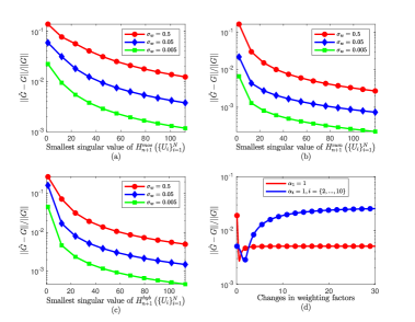
Figure 2: Identification errors under different settings. (a)-(c) Identification results using the MCPE, CCPE, and HCPE conditions, respectively, across different noise levels and synthetic matrix singular value settings. (d) Identification results for the MCPE condition under various weighting factor configurations.

For the MCPE condition, the data sets can have varying dimensions but must satisfy $\sum_{i=1}^{N}T_{i}\geq 50$ (see Theorem 2). Control sequence lengths are randomly generated within the range [5, 14]. For the CCPE condition, the ten data sets must have identical dimensions and satisfy $T_{0}\geq 14$ (see Theorem 2), we set $T_{0}=25$. For the HCPE condition, partial dimensional consistency is allowed $\bar{p}=3$, with the condition $T_{0}+\sum_{i=\bar{p}}^{p}T_{i}\geq 5L-3$ (see Theorem 2). Let $T_{0}=10$, the remaining controller lengths are randomly generated within [5, 14].

The input sequences for all three conditions are designed using the method in Section 4. The initial state values are randomly generated within the range [-1, 1]. Additionally, the standard deviation of the process noise $\sigma_{w}$ is varied from $0$ to $0.1$. The weighting factors for each CPE condition are fixed as $\alpha_{i}=1$ for $i=1,2,\dots,10$. The identification errors under various conditions are shown in Fig. 2(a)-(c). The results validate the effectiveness of the three synthesized conditions for least-squares identification. The identification error decreases as the minimum singular value of the synthesized matrix increases, which is consistent with the result of Theorem 3.

To highlight the significance of weighting factors, we examined scenarios where $\alpha_{1}$ and $\alpha_{2}-\alpha_{10}$ varied within the range (0, 30] under the MCPE condition. The results, corresponding to a noise level of $\sigma_{w}=0.05$, are presented in Fig. 2(d). The red line represents the case where $\alpha_{1}$ varies while $\alpha_{2}-\alpha_{10}$ remain fixed at 1, whereas the blue line represents the case where $\alpha_{1}$ is fixed at 1 and $\alpha_{2}-\alpha_{10}$ vary synchronously. The findings indicate that significant disparities in signal magnitudes under the MCPE condition can degrade discrimination performance. Conversely, an appropriate selection of weighting factors effectively mitigates identification errors.

6.2 State Feedback Controller Design Using Parametric Modeling Approach

In this subsection, we apply the data-driven state feedback design method described in [10] to the system defined by (6.1) using the three CPE conditions. Specifically, taking the CCPE condition as an example. Utilizing the approach in [10, Th. 3], the design challenge for stabilizing controllers is transformed into an LMI problem for any matirx $Q$:

$$\begin{bmatrix}{{H_{1}^{cum}(\{{x_{i}^{[0,{T_{0}-1}]}\}_{i=1}^{p}})}Q}&{{H_{1}^{cum}(\{{x_{i}^{[1,{T_{0}}]}\}_{i=1}^{p}})}Q}\\ {{{\left({{H_{1}^{cum}(\{{x_{i}^{[1,{T_{0}}]}\}_{i=1}^{p}})}Q}\right)}^{T}}}&{{H_{1}^{cum}(\{{x_{i}^{[0,{T_{0}-1}]}\}_{i=1}^{p}})}Q}\end{bmatrix}>0,$$ (19)

and the feedback control gain can be obtained by

$$K= {H_{1}^{cum}(\{{u_{i}^{[0,{T_{0}-1}]}\}_{i=1}^{p}})}Q$$

$$~~~~~~~~~~~~~~~~~~~\times{\left({{H_{1}^{cum}(\{{x_{i}^{[0,{T_{0}-1}]}\}_{i=1}^{p}})}Q}\right)^{-1}}.$$ (20)

For this example, we use the control signals generated in the previous subsection as a priori control inputs to generate corresponding input-state trajectories for the three CPE conditions.

In the case of the CCPE condition, the collected input-state trajectories are synthesized into ${H_{1}^{cum}(\{{u_{i}^{[0,{T_{0}-1}]}\}_{i=1}^{p}})}$, ${H_{1}^{cum}(\{{x_{i}^{[0,{T_{0}-1}]}\}_{i=1}^{p}})}$, and ${H_{1}^{cum}(\{{x_{i}^{[1,{T_{0}}]}\}_{i=1}^{p}})}$. These matrices are then processed using MATLAB’s LMI toolbox [31] to compute the control gain $K_{cum}$:

$${K_{cum}}=\begin{bmatrix}{0.8480}&{-1.4693}&{0.1463}&{-1.5678}\\ {4.0457}&{0.0394}&{3.2812}&{-1.4414}\end{bmatrix}.$$

It can be verified that the closed-loop matrix $A+BK_{cum}$ is stable with a spectral radius of $0.5922$.

For the MCPE condition, the collected input-state trajectories are synthesized into ${H_{1}^{mos}(\{{u_{i}^{[0,{T_{i}-1}]}\}_{i=1}^{p}})}$, ${H_{1}^{mos}(\{{x_{i}^{[0,{T_{i}-1}]}\}_{i=1}^{p}})}$, and ${H_{1}^{mos}(\{{x_{i}^{[1,{T_{i}}]}\}_{i=1}^{p}})}$, and these matrices replace the corresponding matrices in (19) and (6.2). Solving the resulting LMI yields the control gain $K_{mos}$:

$${K_{mos}}=\begin{bmatrix}{0.8218}&{-1.4683}&{0.1403}&{-1.5406}\\ {3.9691}&{0.0432}&{3.2652}&{-1.3369}\end{bmatrix}.$$

It can be verified that the closed-loop matrix $A+BK_{mos}$ is stable with a spectral radius of $0.5921$.

Finally for the HCPE condition, the resulting input-state trajectories are organized into ${H_{1}^{hyb}(\{{u_{i}^{[0,{T_{i}-1}]}\}_{i=1}^{p}})}$, ${H_{1}^{hyb}(\{{x_{i}^{[0,{T_{i}-1}]}\}_{i=1}^{p}})}$, and ${H_{1}^{hyb}(\{{x_{i}^{[1,{T_{i}}]}\}_{i=1}^{p}})}$, replacing the corresponding matrices in (19) and (6.2). Solving yields a control gain $K_{hyb}$:

$${K_{hyb}}=\begin{bmatrix}{0.8416}&{-1.4690}&{0.1450}&{-1.5594}\\ {4.0254}&{0.0399}&{3.2761}&{-1.4282}\end{bmatrix}.$$

It can be verified that the closed-loop matrix $A+BK_{hyb}$ is stable with a spectral radius of $0.5942$.

7 Conclution

In this paper, we have developed and analyzed three collectively persistently exciting (CPE) conditions, each incorporating weight factors, from the perspectives of same-dimensional, different-dimensional, and partially same-dimensional data. We argue that these three CPE conditions offer valuable insights for designing data-driven methodologies tailored to diverse multi-signal control scenarios, including those involving signals with insufficient informativeness. We have explored the interrelations between these conditions and examined their rank properties within the framework of linear time-invariant systems. To address the challenges of insufficient information in signal segments, we have proposed open-loop experimental design methods tailored to each CPE condition, enabling the synthesis of the required excitation conditions both offline or online. The effectiveness of these CPE conditions has been demonstrated in the context of least-squares identification, where all three conditions successfully extend Willems’ fundamental lemma. Illustrative examples show that these conditions lead to satisfactory results in both model identification and the development of data-driven controllers.

Several topics for future research remain open. An interesting but challenging extension lies in devising data-driven control methods in a distributed framework, as opposed to a centralized one, while ensuring adherence to the three CPE conditions with multiple control signals. Furthermore, we note that weighting factors have an impact on the performance and effectiveness of data-driven methods. Therefore, how to systematically design optimal weighting factors for data-driven problems is another direction worth exploring.

Appendix

7.1 Proof of Theorem 1

1). If $\{z_{i}^{[0,{T_{i}-1}]}\}_{i=1}^{p}$ are CCPE, then $T_{0}=T_{1}=T_{2}=...=T_{p}$ and ${H_{L}^{cum}(\{{z_{i}^{[0,{T_{i}-1}]}\}_{i=1}^{p}})}{{H_{L}^{cum}(\{{z_{i}^{[0,{T_{i}-1}]}\}_{i=1}^{p}})}}^{T}>0$, i.e.,

$$\sum\limits_{i=1}^{p}{\left({{\alpha_{i}}{H_{L}}({z_{i}^{[0,{T_{i}}-1]}})\sum\limits_{i\neq j=1}^{p}{{\alpha_{j}}H_{L}^{T}({z_{j}^{[0,{T_{j}}-1]}})}}\right)}$$

$$~~~~~~~~~~+\underbrace{\alpha_{i}^{2}\sum\limits_{i=1}^{p}{{H_{L}}({z_{i}^{[0,{T_{i}}-1]}})H_{L}^{T}({z_{i}^{[0,{T_{i}}-1]}})}}_{M_{1}}>0.$$ (21)

In order to establish the full row rank of ${H_{L}^{mos}(\{{z_{i}^{[0,{T_{i}-1}]}\}_{i=1}^{p}})}$, it is sufficient to show the positivity of $M_{1}$. Given $\sum\limits_{i=1}^{p}{{H_{L}}({z_{i}^{[0,{T_{i}}-1]}})H_{L}^{T}({z_{i}^{[0,{T_{i}}-1]}})}\geq 0$ and $\alpha_{i}\neq 0$, if there exists a non-zero vector $x$ such that $x\in\ker M_{1}$, then we must have $H_{L}^{T}({z_{1}^{[0,{T_{i}}-1]}})x=\cdots H_{L}^{T}({z_{p}^{[0,{T_{i}}-1]}})x=0$, implying

$$x\in\ker\sum\limits_{i=1}^{p}{\left({{\alpha_{i}}{H_{L}}({z_{i}^{[0,{T_{i}}-1]}})\sum\limits_{i\neq j=1}^{p}{{\alpha_{j}}H_{L}^{T}({z_{j}^{[0,{T_{j}}-1]}})}}\right)}.$$

This conclusion contradicts inequality (7.1). Therefore $M_{1}>0$. Consequently, $\{z_{i}^{[0,{T_{i}-1}]}\}_{i=1}^{p}$ are also MCPE.

Since ${H_{L}^{cum}(\{{z_{i}^{[0,{T_{i}-1}]}\}_{i=1}^{p}})}={H_{L}^{cum}(\{{z_{i}^{[0,{T_{i}-1}]}\}_{i=1}^{\bar{p}}})}+{H_{L}^{cum}(\{{z_{i}^{[0,{T_{i}-1}]}\}_{i=\bar{p}+1}^{p}})}$, the method employed above to establish the full row rank of ${H_{L}^{mos}(\{{z_{i}^{[0,{T_{i}-1}]}\}_{i=1}^{p}})}$ from the full row rank matrix ${H_{L}^{cum}(\{{z_{i}^{[0,{T_{i}-1}]}\}_{i=1}^{p}})}$ is also applicable to determining the full row rank of ${\begin{bmatrix}{H_{L}^{cum}(\{z^{[0,T_{0}-1]}_{i}\}_{i=1}^{\bar{p}})}&{H_{L}^{mos}(\{z^{[0,T_{i}-1]}_{i}\}_{i=\bar{p}+1}^{p})}\end{bmatrix}}$ from the full row rank matrix ${H_{L}^{cum}(\{{z_{i}^{[0,{T_{i}-1}]}\}_{i=1}^{\bar{p}}})}+{H_{L}^{cum}(\{{z_{i}^{[0,{T_{i}-1}]}\}_{i=\bar{p}+1}^{p}})}$. Therefore $\{z_{i}^{[0,{T_{i}-1}]}\}_{i=1}^{p}$ are also HCPE.

2). i). If $\{z_{i}^{[0,{T_{i}-1}]}\}_{i=1}^{p}$ are MCPE and $T_{0}=T_{1}=T_{2}=...=T_{p}$, we have ${H_{L}^{cum}(\{{z_{i}^{[0,{T_{i}-1}]}\}_{i=1}^{p}})}={H_{L}^{mos}(\{{z_{i}^{[0,{T_{i}-1}]}\}_{i=1}^{p}})}({\textbf{1}_{p}}\otimes{I_{{T_{0}}-L+1}})$. Then,

$$\text{rank}\ {H_{L}^{cum}(\{{z_{i}^{[0,{T_{i}-1}]}\}_{i=1}^{p}})}=\text{rank}\ {H_{L}^{mos}(\{{z_{i}^{[0,{T_{i}-1}]}\}_{i=1}^{p}})}$$

$$~~~-~\text{dim}[\text{im}\,{H_{L}^{mos}(\{{z_{i}^{[0,{T_{i}-1}]}\}_{i=1}^{p}})^{T}}\cap\text{im}({{\bf{1}}_{p}}\otimes{I_{{T_{0}}-L+1}})^{\perp}].$$

Thus, we have

$$\text{rank}\ {H_{L}^{cum}(\{{z_{i}^{[0,{T_{i}-1}]}\}_{i=1}^{p}})}=\text{rank}\ {H_{L}^{mos}(\{{z_{i}^{[0,{T_{i}-1}]}\}_{i=1}^{p}})}$$

if $\text{im}\,{H_{L}^{mos}(\{{z_{i}^{[0,{T_{i}-1}]}\}_{i=1}^{p}})^{T}}\cap\text{leftker}\,{\textbf{1}_{p}}\otimes{I_{{T_{0}}-L+1}}=\{0\}$, i.e., $\{z_{i}^{[0,{T_{i}-1}]}\}_{i=1}^{p}$ are also CCPE.

2). ii). If $T_{0}=T_{1}=T_{2}=...=T_{\bar{p}}$, we have

$${H_{L}^{hyb}(\{{z_{i}^{[0,{T_{i}-1}]}\}_{i=1}^{p}})}$$

$$~~~~={H_{L}^{mos}(\{{z_{i}^{[0,{T_{i}-1}]}\}_{i=1}^{\bar{p}}})}(\begin{bmatrix}{{\textbf{1}_{\bar{p}}}}&{{0_{\bar{p}\times(p-\bar{p})}}}\\ {{0_{p-\bar{p}}}}&{{I_{p-\bar{p}}}}\end{bmatrix}\otimes{I_{{T_{0}}-L+1}}).$$

Similarly to the above, if additionally, $\text{im}\,{{H_{L}^{mos}(\{{z_{i}^{[0,{T_{i}-1}]}\}_{i=1}^{\bar{p}}})}^{T}}\cap\text{leftker}\,{\begin{bmatrix}{{\textbf{1}_{\bar{p}}}}&{{0_{\bar{p}\times(p-\bar{p})}}}\\ {{0_{p-\bar{p}}}}&{{I_{p-\bar{p}}}}\end{bmatrix}}\otimes{I_{{T_{0}}-L+1}}=\{0\}$, then $\{z_{i}^{[0,{T_{i}-1}]}\}_{i=1}^{p}$ are HCPE.

3). i). If $\{z_{i}^{[0,{T_{i}-1}]}\}_{i=1}^{p}$ are HCPE, then $T_{0}=T_{1}=...=T_{\bar{p}}$ and ${H_{L}^{hyb}(\{z^{[0,T_{i}-1]}_{i}\}_{i=1}^{p})}{H_{L}^{hyb}(\{z^{[0,T_{i}-1]}_{i}\}_{i=1}^{p})}^{T}>0$, i.e., ${M_{1}}+\sum\limits_{i=1}^{\bar{p}}{\left({{\alpha_{i}}{H_{L}}({z_{i}^{[0,{T_{0}}-1]}})\sum\limits_{i\neq j=1}^{\bar{p}}{{\alpha_{j}}H_{L}^{T}({z_{j}^{[0,{T_{0}}-1]}})}}\right)}>0$. Similar to the proof of conclusion 1), we can deduce $M_{1}>0$, and thus $\{z_{i}^{[0,{T_{i}-1}]}\}_{i=1}^{p}$ are also MCPE.

3). ii). If $T_{0}=T_{\bar{p}+1}=...=T_{p}$, then ${H_{L}^{hyb}(\{{z_{i}^{[0,{T_{i}-1}]}\}_{i=1}^{p}})}$ can be regarded as a special case of ${H_{L}^{mos}(\{{z_{i}^{[0,{T_{i}-1}]}\}_{i=1}^{p}})}$ in conclusion 2). i). The proof for this case is evidently straightforward. $\blacksquare$

[]Ao Cao received the B.S. degree in automation from the Wuhan University of Technology, Wuhan, China, in 2021. He is currently pursuing the Ph.D. degree in control science and engineering from the College of Artificial Intelligence, Nankai University, Tianjin, China. His current research interests include multi-agent systems, data-driven control, and reinforcement learning.

[]Fuyong Wang received the Ph.D. degree in control science and engineering from Nankai University, Tianjin, China, in 2019. He is currently an Associate Professor with the Department of Automation, Nankai University. His current research interests include distributed learning, control and optimization of multi-agent systems, security analysis and control of cyber-physical systems, cooperative perception, decision-making and planning of multi-robot systems.

References

- [1] J. C. Willems, P. Rapisarda, I. Markovsky, and B. L. De Moor, “A note on persistency of excitation,” Systems & Control Letters, vol. 54, no. 4, pp. 325–329, 2005.
- [2] P. Ioannou and B. Fidan, Adaptive Control Tutorial. SIAM, 2006.
- [3] T. Katayama et al., Subspace Methods for System Identification. Springer, 2005, vol. 1.
- [4] I. Markovsky, J. C. Willems, P. Rapisarda, and B. L. De Moor, “Algorithms for deterministic balanced subspace identification,” Automatica, vol. 41, no. 5, pp. 755–766, 2005.
- [5] I. Markovsky, Low Rank Approximation: Algorithms, Implementation, Applications. Springer, 2012, vol. 906.
- [6] M. Lovera, T. Gustafsson, and M. Verhaegen, “Recursive subspace identification of linear and non-linear Wiener state-space models,” Automatica, vol. 36, no. 11, pp. 1639–1650, 2000.
- [7] J. Berberich, J. Köhler, M. A. Müller, and F. Allgöwer, “Data-driven model predictive control with stability and robustness guarantees,” IEEE Transactions on Automatic Control, vol. 66, no. 4, pp. 1702–1717, 2021.
- [8] J. Bongard, J. Berberich, J. Köhler, and F. Allgöwer, “Robust stability analysis of a simple data-driven model predictive control approach,” IEEE Transactions on Automatic Control, vol. 68, no. 5, pp. 2625–2637, 2023.
- [9] W. Liu, J. Sun, G. Wang, F. Bullo, and J. Chen, “Data-driven resilient predictive control under denial-of-service,” IEEE Transactions on Automatic Control, vol. 68, no. 8, pp. 4722–4737, 2023.
- [10] C. De Persis and P. Tesi, “Formulas for data-driven control: Stabilization, optimality, and robustness,” IEEE Transactions on Automatic Control, vol. 65, no. 3, pp. 909–924, 2020.
- [11] U. S. Park and M. Ikeda, “Stability analysis and control design of LTI discrete-time systems by the direct use of time series data,” Automatica, vol. 45, no. 5, pp. 1265–1271, 2009.
- [12] B. Nortmann and T. Mylvaganam, “Direct data-driven control of linear time-varying systems,” IEEE Transactions on Automatic Control, vol. 68, no. 8, pp. 4888–4895, 2023.
- [13] M. Gevers, A. S. Bazanella, X. Bombois, and L. Miskovic, “Identification and the information matrix: How to get just sufficiently rich?” IEEE Transactions on Automatic Control, vol. 54, no. 12, pp. 2828–2840, 2009.
- [14] H. J. van Waarde, J. Eising, H. L. Trentelman, and M. K. Camlibel, “Data informativity: A new perspective on data-driven analysis and control,” IEEE Transactions on Automatic Control, vol. 65, no. 11, pp. 4753–4768, 2020.
- [15] S. Kang and K. You, “Minimum input design for direct data-driven property identification of unknown linear systems,” Automatica, vol. 156, p. 111130, 2023.
- [16] H. J. Van Waarde, J. Eising, M. K. Camlibel, and H. L. Trentelman, “The informativity approach: To data-driven analysis and control,” IEEE Control Systems Magazine, vol. 43, no. 6, pp. 32–66, 2023.
- [17] S. Aranovskiy, A. Bobtsov, R. Ortega, and A. Pyrkin, “Parameters estimation via dynamic regressor extension and mixing,” in 2016 American Control Conference (ACC), 2016, pp. 6971–6976.
- [18] R. Ortega, S. Aranovskiy, A. A. Pyrkin, A. Astolfi, and A. A. Bobtsov, “New results on parameter estimation via dynamic regressor extension and mixing: Continuous and discrete-time cases,” IEEE Transactions on Automatic Control, vol. 66, no. 5, pp. 2265–2272, 2021.
- [19] A. Dhar, S. B. Roy, and S. Bhasin, “Initial excitation based discrete-time multi-model adaptive online identification,” European Journal of Control, vol. 68, p. 100672, 2022, 2022 European Control Conference Special Issue.
- [20] W. Chen, C. Wen, S. Hua, and C. Sun, “Distributed cooperative adaptive identification and control for a group of continuous-time systems with a cooperative PE condition via consensus,” IEEE Transactions on Automatic Control, vol. 59, no. 1, pp. 91–106, 2014.
- [21] S. Xie and L. Guo, “Analysis of normalized least mean squares-based consensus adaptive filters under a general information condition,” SIAM Journal on Control and Optimization, vol. 56, no. 5, pp. 3404–3431, 2018.
- [22] I. Markovsky and R. Pintelon, “Identification of linear time-invariant systems from multiple experiments,” IEEE Transactions on Signal Processing, vol. 63, no. 13, pp. 3549–3554, 2015.
- [23] C. De Persis and P. Tesi, “Designing experiments for data-driven control of nonlinear systems,” IFAC-PapersOnLine, vol. 54, no. 9, pp. 285–290, 2021.
- [24] H. J. van Waarde, “Beyond persistent excitation: Online experiment design for data-driven modeling and control,” IEEE Control Systems Letters, vol. 6, pp. 319–324, 2022.
- [25] X. Bombois, G. Scorletti, M. Gevers, P. Van den Hof, and R. Hildebrand, “Least costly identification experiment for control,” Automatica, vol. 42, no. 10, pp. 1651–1662, 2006.
- [26] H. Hjalmarsson, “From experiment design to closed-loop control,” Automatica, vol. 41, no. 3, pp. 393–438, 2005.
- [27] H. J. van Waarde, C. De Persis, M. K. Camlibel, and P. Tesi, “Willems’ fundamental lemma for state-space systems and its extension to multiple datasets,” IEEE Control Systems Letters, vol. 4, no. 3, pp. 602–607, 2020.
- [28] Y. Yu, S. Talebi, H. J. van Waarde, U. Topcu, M. Mesbahi, and B. Açıkmeșe, “On controllability and persistency of excitation in data-driven control: Extensions of Willems’ fundamental lemma,” in 2021 60th IEEE Conference on Decision and Control (CDC), 2021, pp. 6485–6490.
- [29] I. Markovsky and F. Dörfler, “Behavioral systems theory in data-driven analysis, signal processing, and control,” Annual Reviews in Control, vol. 52, pp. 42–64, 2021.
- [30] ——, “Identifiability in the behavioral setting,” IEEE Transactions on Automatic Control, vol. 68, no. 3, pp. 1667–1677, 2023.
- [31] G.-R. Duan and H.-H. Yu, LMIs in Control Systems: Analysis, Design and Applications. CRC press, 2013.
[![[Uncaptioned image]](/html/2501.10030/assets/x4.png) ]Ao Cao received the B.S. degree in automation from the Wuhan University of Technology, Wuhan, China, in 2021. He is currently pursuing the Ph.D. degree in control science and engineering from the College of Artificial Intelligence, Nankai University, Tianjin, China. His current research interests include multi-agent systems, data-driven control, and reinforcement learning.