Tensor meson transition form factors in holographic QCD and the muon $g-2$

Abstract

Despite the prominence of tensor mesons in photon-photon collisions, until recently their contribution to the hadronic light-by-light scattering part of the anomalous magnetic moment of the muon has been estimated at the level of only a few $10^{-12}$, with an almost negligible contribution to the error budget of the Standard Model prediction. A recent reanalysis within the dispersive approach has found that after resolving the issue of kinematic singularities in previous approaches, a larger result is obtained, a few $10^{-11}$, and with opposite sign as in previous results, when a simple quark model for the transition form factors is employed. In this paper, we present the first complete evaluation of tensor meson contributions within a hard-wall model in holographic QCD, which reproduces surprisingly well mass, two-photon width, and the observed singly virtual transition form factors of the dominant $f_{2}(1270)$, requiring only that the energy-momentum tensor correlator is matched to the leading OPE result of QCD. Due to a second structure function that is absent in the quark model, the result for $a_{\mu}$ turns out to be positive instead of negative, and also with a magnitude of a few $10^{-11}$. We discuss both pole and non-pole contributions arising from tensor meson exchanges in the holographic light-by-light scattering amplitude, finding that keeping all contributions improves dramatically the convergence of a sum over excited tensor mesons and avoids unnaturally large contributions from the first few excited modes at low energies. Doing so, the contribution from the lightest tensor mode becomes $a_{\mu}^{T}=5.9\times 10^{-11}$ ($5.4\times 10^{-11}$ from virtualities less than 1.5 GeV).

I Introduction

With the upcoming release of the final result of the Fermilab experiment measuring the anomalous magnetic moment of the muon that is expected to reduce the current experimental error of $22\times 10^{-11}$ in $a_{\mu}=(g-2)_{\mu}/2$ by about a factor of 2, there is currently a world-wide effort to reduce also the uncertainties of the Standard Model prediction which are dominated by hadronic contributions, foremost from hadronic vacuum polarization (HVP), but also from hadronic light-by-light scattering (HLBL) with an error budget of $19\times 10^{-11}$ according to the 2020 White Paper of the Muon $g-2$ Theory Initiative [1].

In the meantime, significant progress has been made regarding the various parts of the HLBL amplitude, in particular regarding the contribution of axial vector mesons and short distance constraints [2, 3, 4, 5, 6]. Different approaches, involving dispersion relations [7, 8, 9, 10], Dyson-Schwinger/Bethe-Salpeter equations [11, 12, 13], resonant chiral models [14, 15, 16], as well as holographic QCD [17, 18, 19, 20, 21] have been employed with results that are sufficiently in agreement to permit an improved estimate with substantially reduced theoretical errors.

A contribution where a rigorous dispersive analysis is not yet available is the one of tensor mesons, where $f_{2}(1270)$ and $a_{2}(1320)$ have sufficiently strong coupling to two photons such that they should be taken into account, since they are too light to be accounted for by the quark-loop contribution which provides sufficiently good accuracy for virtualities higher than about 1.5 GeV.

In [22] the contribution of the tensor mesons $f_{2}(1270)$ and $a_{2}(1320)$ has been estimated with a quark model ansatz for the transition form factor (TFF) [23] as $+0.50(3)\times 10^{-11}$ and $+0.14(3)\times 10^{-11}$, respectively, and a very similar result of $+0.6\times 10^{-11}$ has recently been obtained by using holographic QCD as a model in [24], however in an expressly incomplete evaluation. Recently, larger results with an opposite sign have been obtained in a new dispersive analysis using a formalism that avoids the kinematic singularities present in previous approaches [25], amounting to $-2.5(3)\times 10^{-11}$ in the low-energy region bounded by 1.5 GeV.

In this note we present our results for a complete evaluation of the HLBL contribution obtained by employing the holographic results for the TFF of tensor mesons in a hard-wall model, which has been found to work well in other applications involving TFFs of pseudoscalars and axial vector mesons. As found already in [26], a hard-wall AdS/QCD model where the energy-momentum tensor correlator is matched to the leading OPE result of QCD reproduces the mass of the dominant $f_{2}(1270)$ within 3%, and its two-photon width completely within experimental errors. As shown already in [24] for the helicity-2 amplitude, and extended here to all helicities, the singly virtual transition form factors agree quite well with data from the Belle collaboration [27]. Using the complete set of tensor TFFs that is obtained in hQCD in the formulae of the dispersive approach, we obtain a significantly larger positive result than the holographic study of Ref. [24], larger in absolute value also than the result of Ref. [25].

We also consider a full evaluation beyond the pole contribution as defined by the dispersive approach with optimized basis [28], by keeping the complete HLBL amplitude as given by the holographic model. In contrast to the case of pseudoscalar and axial vector mesons, where the complete HLBL amplitude yields an $a_{\mu}$ contribution identical to the dispersively defined pole contribution, for tensor mesons the resulting formulae differ, and an even larger positive result is obtained.

The holographic model provides also an infinite tower of tensor meson resonances, and we find that summing over these contributions gives a still slightly larger result, with the bulk of the contribution still coming from the region below 1.5 GeV. Summing over the first few modes, we find a similar total result, but if this sum is carried out with only the pole contribution, the convergence is rather slow, with unnaturally large contributions from the excited tensor modes even at low energies.

This paper is organized as follows. In Sec. II, we recall the basic formulae for transition form factors of tensor mesons, following the notation of [29]. In Sec. III, we set up the hard-wall AdS/QCD model used by us and we fix its parameters, which involve only the $\rho$ mass, a five-dimensional flavor-gauge theory coupling fixed by matching to OPE of the vector-vector correlation function, and a five-dimensional Newton constant fixed by matching the OPE of the energy-momentum-tensor correlator in $N_{f}=3$ QCD. In Sec. IV we derive the holographic result for the tensor meson TFFs and we compare with the experimental data of [27], before evaluating both the $a_{\mu}^{\mathrm{HLBL}}$ contribution resulting from the singlet tensor meson as it is naturally present in the model and also when used as a model with refitted masses and two-photon widths to match $f_{2}(1270)$, $a_{2}(1320)$, and $f_{2}^{\prime}(1525)$. The $a_{\mu}$ contributions are evaluated both with a restriction to the pole term as defined by the dispersive approach in the optimized basis of Ref. [28] and without. The corresponding formulae are given in Appendix A.

II Transition form factor of tensor mesons

The matrix element of a massive tensor meson decaying into two off-shell photons is given by

$$\langle\gamma^{*}(q_{1},\lambda_{1})\gamma^{*}(q_{2},\lambda_{2})|T(p,\lambda_{T})\rangle=$$ (1)

$$i(2\pi)^{4}\delta^{(4)}(q_{1}+q_{2}-p)e^{2}{\epsilon_{\mu}^{\lambda_{1}}}^{*}(q_{1}){\epsilon_{\nu}^{\lambda_{2}}}^{*}(q_{2})\epsilon_{\alpha\beta}^{\lambda_{T}}(p)\mathcal{M}^{\mu\nu\alpha\beta}(q_{1},q_{2}),$$

with

$$\epsilon_{\alpha\beta}^{\lambda_{T}}(p)\mathcal{M}^{\mu\nu\alpha\beta}(q_{1},q_{2})$$

$$=i\int d^{4}x\,e^{iq_{1}\cdot x}\langle 0|T\{j_{\mathrm{em}}^{\mu}(x)j_{\mathrm{em}}^{\nu}(0)\}|T(p,\lambda_{T})\rangle.$$ (2)

The expressions of the massive tensor polarization $\epsilon_{\alpha\beta}^{\lambda_{T}}$ can be found in [30, 29]. The sum over polarizations gives the projector

$$s^{T}_{\alpha\beta\alpha^{\prime}\beta^{\prime}}(p) =\sum_{\lambda_{T}}\epsilon_{\alpha\beta}^{\lambda_{T}}(p)\epsilon_{\alpha^{\prime}\beta^{\prime}}^{\lambda_{T}}(p)^{*}$$

$$=\frac{1}{2}\left(s_{\alpha\beta^{\prime}}s_{\alpha^{\prime}\beta}+s_{\alpha\alpha^{\prime}}s_{\beta\beta^{\prime}}\right)-\frac{1}{3}s_{\alpha\beta}s_{\alpha^{\prime}\beta^{\prime}},$$ (3)

where

$$s_{\alpha\alpha^{\prime}}=-\left(g_{\alpha\alpha^{\prime}}-\frac{p_{\alpha}p_{\alpha^{\prime}}}{m_{T}^{2}}\right),$$ (4)

satisfies

$$\eta^{\alpha^{\prime}\alpha^{\prime\prime}}\eta^{\beta^{\prime}\beta^{\prime\prime}}s^{T}_{\alpha\beta\alpha^{\prime}\beta^{\prime}}s^{T}_{\alpha^{\prime\prime}\beta^{\prime\prime}\alpha^{\prime\prime\prime}\beta^{\prime\prime\prime}}=s^{T}_{\alpha\beta\alpha^{\prime\prime\prime}\beta^{\prime\prime\prime}},$$ (5)

and enters in the expression of the massive tensor (Fierz-Pauli) propagator

$$G^{T}_{\alpha\beta,\alpha^{\prime}\beta^{\prime}}=\frac{s^{T}_{\alpha\beta\alpha^{\prime}\beta^{\prime}}(p)}{p^{2}-m_{T}^{2}}.$$ (6)

In the literature, there are two widely used choices of basis of tensor structures. One is aimed at explicitly selecting amplitudes of given helicity [30], more directly related to experiments. while the second choice follows the so called BTT construction [31, 32], used in the data driven dispersive approach, which aims at obtaining a decomposition of the transition form factors, with scalar coefficients not having kinematical singularities [29].

Following the second approach, Lorentz and gauge invariance with respect to photon momenta, crossing symmetry requirement

$$\mathcal{M}^{\mu\nu\alpha\beta}(q_{1},q_{2})=\mathcal{M}^{\nu\mu\alpha\beta}(q_{2},q_{1}),$$ (7)

and the observation that only those structures that do not vanish upon contraction with the projector $s^{T}_{\alpha\beta\alpha^{\prime}\beta^{\prime}}$ can contribute to observables involving on-shell tensor mesons narrows the choice to five independent tensor structures. (Levi-Civita tensor structures are excluded by parity conservation):

$$T_{1}^{\mu\nu\alpha\beta} = g^{\mu\alpha}P_{21}^{\nu\beta}+g^{\nu\alpha}P_{12}^{\mu\beta}+g^{\mu\beta}P_{21}^{\nu\alpha}$$

$$+ g^{\nu\beta}P_{12}^{\mu\alpha}+g^{\mu\nu}(q_{1}^{\alpha}q_{2}^{\beta}+q_{2}^{\alpha}q_{1}^{\beta})$$

$$- q_{1}\cdot q_{2}(g^{\mu\alpha}g^{\nu\beta}+g^{\nu\alpha}g^{\mu\beta}),$$

$$T_{2}^{\mu\nu\alpha\beta} = (q_{1}^{\alpha}q_{1}^{\beta}+q_{2}^{\alpha}q_{2}^{\beta})P_{12}^{\mu\nu},$$

$$T_{3}^{\mu\nu\alpha\beta} = P_{11}^{\mu\alpha}P_{22}^{\nu\beta}+P_{11}^{\mu\beta}P_{22}^{\nu\alpha},$$ (8)

$$T_{4}^{\mu\nu\alpha\beta} = P_{12}^{\mu\alpha}P_{22}^{\nu\beta}+P_{12}^{\mu\beta}P_{22}^{\nu\alpha},$$

$$T_{5}^{\mu\nu\alpha\beta} = P_{21}^{\nu\alpha}P_{11}^{\mu\beta}+P_{21}^{\nu\beta}P_{11}^{\mu\alpha},$$

where

$$P_{ij}^{\mu\nu}=g^{\mu\nu}q_{i}\cdot q_{j}-q_{i}^{\nu}q_{j}^{\mu}.$$ (9)

Thus, the tensor TFF depends on five scalar coefficients $\mathcal{F}_{i}(q_{1}^{2},q_{2}^{2})$:

$$\mathcal{M}^{\mu\nu\alpha\beta}=\sum_{i=1}^{5}\frac{\mathcal{F}_{i}^{T}}{m_{T}^{n_{i}}}T_{i}^{\mu\nu\alpha\beta},$$ (10)

where $n_{1}=1,n_{i}=3\;\text{for}\;j=2,...,5$, so that the all the $\mathcal{F}_{i}$ are dimensionless.

Only $\mathcal{F}_{1}$ and $\mathcal{F}_{2}$ enter the on-shell photon result

$$\Gamma_{T\rightarrow\gamma\gamma}=\frac{\pi\alpha^{2}m_{T}}{5}\left(|\mathcal{F}_{1}^{T}(0,0)|^{2}+\frac{1}{24m_{T}^{6}}|\mathcal{F}_{2}^{T}(0,0)|^{2}\right).$$ (11)

In singly virtual TFFs, all $\mathcal{F}^{T}_{i}$ contribute, except for $\mathcal{F}^{T}_{3}$, unless the latter has a singularity at zero virtualities.

In previous studies of the contribution of tensor mesons to HLBL scattering and to $a_{\mu}$, only the simple quark model ansatz of Ref. [23] for $\mathcal{F}^{T}_{1}$, with the remaining $\mathcal{F}^{T}_{i}$ set to zero, has been employed:

$$\mathcal{F}^{T}_{1}(-Q_{1}^{2},-Q_{2}^{2})=\frac{\mathcal{F}^{T}_{1}(0,0)}{(1+(Q_{1}^{2}+Q_{2}^{2})/\Lambda_{T}^{2})^{2}}.$$ (12)

In the following we shall employ holographic QCD as a model for the TFFs of mesons and compare with the results obtained by the quark model with common choices of $\Lambda_{T}$.

III AdS/QCD

Holographic QCD models [33, 34, 35, 36, 37] have been constructed along the lines of the original conjectured AdS/CFT duality (equivalence) between a four-dimensional (4D) (conformal) large-N_c gauge theory at strong coupling and a (classical) five-dimensional (5D) field theory in a curved gravitational background with Anti-de-Sitter metric [38], which can be summarized as follows [39, 40]: for every quantum operator ${\cal O}(x)$ of the 4D (strongly coupled) gauge theory, there exists a corresponding 5D field $\phi(x,z)$, whose value on the conformal boundary (taken at $z=\epsilon\to 0$) $\phi(x,0)\equiv\phi_{0}(x)$, is identified, modulo some specific powers of $\epsilon$, with the four-dimensional source of ${\cal O}(x)$. The generating functional of the 4D theory can be computed from the 5D action evaluated on-shell, i.e.:

$$\mbox{exp}\left(iS_{5}[\phi_{0}(x)]\right)=\left\langle\mbox{exp}\left[i\int d^{4}x\,\phi_{0}(x)\,{\cal O}(x)\right]\right\rangle_{\rm QCD_{4}}~.$$ (13)

By varying the action with respect to the 4D boundary values $\phi_{0}(x)$, one generates connected $n$-point Green’s functions of large-$N_{c}$, strong-coupled 4D gauge theory.

We shall introduce a 5D tensor field as a metric deformation in hQCD models together with 5D gauge fields which are used to compute correlators of (conserved) $SU(3)_{L}\times SU(3)_{R}$ (or $U(3)_{L}\times U(3)_{R}$) flavor chiral currents of QCD, in the large-N$c$ limit,

$$J^{a}_{L\,\mu}=\overline{q}_{L}\,\gamma^{\mu}\,T^{a}\,q_{L},\quad J^{a}_{R\,\mu}=\overline{q}_{R}\,\gamma^{\mu}\,T^{a}\,q_{R}$$ (14)

where $T^{a}=\lambda^{a}/2$, with $\lambda^{a}$, $a=1,...8$ being the $SU(3)$ Gell-Mann matrices, augmented by $T^{0}=\textbf{1}_{3}/\sqrt{6}$, such that $\text{tr}\,(T^{a}\,T^{b})=\delta_{ab}/2$.

The 5D action describes a Yang-Mills theory (with a Chern-Simons term which we omit, because it plays no role here) in a curved 5D AdS₅ space, with the extra dimension $z$, extending over the finite interval $(0,z_{0}]$, and metric

$$ds^{2}=z^{-2}(\eta_{\mu\nu}dx^{\mu}dx^{\nu}-dz^{2}).$$ (15)

The 5D Yang-Mills action is given by

$$S_{\rm YM}=-\frac{1}{4g_{5}^{2}}\int d^{4}x\int_{0}^{z_{0}}dz\,\sqrt{-g}\,g^{PR}g^{QS}\,\text{tr}\left(\mathcal{F}^{\mathrm{L}}_{PQ}\mathcal{F}^{\mathrm{L}}_{RS}+\mathcal{F}^{\mathrm{R}}_{PQ}\mathcal{F}^{\mathrm{R}}_{RS}\right),$$ (16)

where $P,Q,R,S=0,\dots,3,z$ and $\mathcal{F}_{MN}=\partial_{M}\mathcal{B}_{N}-\partial_{N}\mathcal{B}_{M}-i[\mathcal{B}_{M},\mathcal{B}_{N}]$, $\mathcal{B}_{N}=L_{N},\;R_{N}$ being 5D gauge fields transforming under $U(3)_{L,R}$ respectively. Vector and axial-vector fields are given by ${V}_{\mu}=\frac{1}{2}({L}_{\mu}+{R}_{\mu})$ and ${A}_{\mu}=\frac{1}{2}({L}_{\mu}-{R}_{\mu})$. Boundary conditions have to be imposed on the 5D vector fields at $z=z_{0}$. For the vector fields, working in the $V_{z}=0$ gauge and imposing the boundary conditions $V_{\mu}(x,0)=0$ and $\partial_{z}V_{\mu}(x,z_{0})=0$, the expansion $V_{\mu}^{a}(x,z)=g_{5}\sum_{n=1}^{\infty}v_{\mu}^{a}(x)\psi_{n}(z)$ is obtained in terms of 4D canonically normalized vector fields $v_{\mu}^{a}(x)$, where the $\psi_{n}(z)$ are solutions of the 5D equation of motions, vanishing at $z=0$ and such that $\partial_{z}\psi_{n}(z)=0$, with normalization $\int_{0}^{z_{0}}dz\,z^{-1}\psi_{n}(z)^{2}=1$, explicitly:

$$\psi_{n}(z)=\sqrt{2}\frac{zJ_{1}(\gamma_{0,n}z/z_{0})}{z_{0}J_{1}(\gamma_{0,n})}.$$ (17)

Masses are given in terms of the zeros of the Bessel function $J_{0}(\gamma_{0,n})=0$ by $m_{n}=\gamma_{0,n}/z_{0}$.

Identifying the mass of the lowest vector resonance with the mass of the $\rho$ meson $m_{1}=\gamma_{0,1}/z_{0}=m_{\rho}=775.26$ MeV fixes

$$z_{0}=\gamma_{0,1}/m_{\rho}=3.102\,\text{GeV}^{-1}.$$ (18)

A fundamental object in a holographic model is the bulk-to-boundary propagator, which is a solution of the vector 5D equation of motion, with $m_{n}^{2}$ replaced by $q^{2}$ and the boundary conditions $\mathcal{J}(Q,0)=1$ and $\partial_{z}\mathcal{J}(Q,z_{0})=0$. For Euclidean momenta $q^{2}=-Q^{2}$, it is given by

$$\mathcal{J}(Q,z)=Qz\left[K_{1}(Qz)+\frac{K_{0}(Qz_{0})}{I_{0}(Qz_{0})}I_{1}(Qz)\right]$$ (19)

Using the holographic recipe, the 4D vector current two-point function can be written in terms of (19), and matching the leading-order pQCD result [34],

$$\Pi_{V}(Q^{2})=-\frac{1}{g_{5}^{2}Q^{2}}\left(\frac{1}{z}\partial_{z}\mathcal{J}(Q,z)\right)\Big{|}_{z\to 0}=-\frac{N_{c}}{24\pi^{2}}\ln Q^{2}+\ldots,$$ (20)

which determines $g_{5}^{2}=12\pi^{2}/N_{c}$.

As already mentioned above, following [26], the tensor meson is introduced in the model as a deformation of the 4D part of the $AdS$ metric

$$ds^{2}=g_{MN}dx^{M}dx^{N}=\frac{1}{z^{2}}(\eta_{\mu\nu}+h_{\mu\nu})dx^{\mu}dx^{\nu}-\frac{1}{z^{2}}dz^{2}\,.$$ (21)

Its dynamics is described by the 5D Einstein-Hilbert action.

$$S_{\mathrm{EH}} = -2k_{T}\int d^{5}x\,\sqrt{g}\,(\mathcal{R}+2\Lambda)$$ (22)

$$= -\frac{k_{T}}{2}\int d^{5}x\,\frac{1}{z^{3}}\eta^{\mu\alpha}\eta^{\nu\beta}(\partial_{z}h_{\mu\nu}\partial_{z}h_{\alpha\beta}+h_{\mu\nu}\Box h_{\alpha\beta}+\ldots)\,,$$

It is possible to fix the value of constant $k_{T}$ in a manner analogous to what was done for $g_{5}$, making the assumption that $h_{\mu\nu}(x,z)$ couples on the conformal boundary $z=0$ to the energy-momentum tensor of QCD fields. Then, the two-point function of the 4D energy-momentum tensor can be identified as

$$\langle T^{\mu\nu}T^{\rho\sigma}\rangle=4\frac{\delta^{2}S_{\mathrm{on-shell}}}{\delta h_{\mu\nu}\delta h_{\rho\sigma}}\to-\frac{1}{2}k_{T}P^{\mu\nu\rho\sigma}Q^{4}\ln Q^{2}$$ (23)

with $P_{\mu\nu\rho\sigma}=\frac{1}{2}(\eta_{\mu\rho}\eta_{\nu\sigma}+\eta_{\mu\sigma}\eta_{\nu\rho}-\frac{2}{3}\eta_{\mu\nu}\eta_{\rho\sigma})$ Matching to the leading term of the OPE of the energy-momentum tensor correlator [26, 41]

$$\langle T^{\mu\nu}T^{\rho\sigma}\rangle_{\mathrm{QCD}}=-P^{\mu\nu\rho\sigma}\left(\frac{N_{c}N_{f}}{160\pi^{2}}+\frac{N_{c}^{2}-1}{80\pi^{2}}\right)Q^{4}\ln Q^{2}+\ldots$$ (24)

determines

$$k_{T}=\left(\frac{N_{c}N_{f}}{80\pi^{2}}+\frac{N_{c}^{2}-1}{40\pi^{2}}\right).$$ (25)

Solutions of traceless-transverse metric fluctuation $h_{\mu\nu}=\epsilon_{\mu\nu}^{T}(q)h_{n}(z)$ with $h_{n}(0)=0=h_{n}^{\prime}(z_{0})$, satisfying the canonical normalization $\frac{k_{T}}{(m^{T}_{n})^{2}}\int dzz^{-3}(\partial_{z}h_{n})^{2}=1$, are given by

$$h_{n}(z)=\displaystyle\frac{\sqrt{2/k_{T}}}{{z_{0}}J_{2}\left(\gamma_{1,n}\right)}z^{2}J_{2}(\gamma_{1,n}z/z_{0}),$$ (26)

yielding a tower of (singlet) tensor meson modes with masses fixed by

$$m_{n}^{T}/m_{\rho}=\gamma_{1,n}/\gamma_{0,1}=1.593,\,2.917,\,4.230,\,\ldots$$ (27)

The lowest tensor resonance mass is thus $m^{T}_{1}=1.235$ GeV, differing by only about $3\%$ from the physical value $M_{f_{2}}=1.2754$ GeV of $f_{2}(1270)$.

IV Holographic Tensor Meson TFF

Photons with polarization vector $\epsilon^{\mu}(q)$, momentum $q$ and virtuality $Q^{2}=-q^{2}$ are described by a vector flavor gauge field involving the vector bulk-to-boundary propagator $\mathcal{J}(z,Q)$ according to (for $N_{f}=3$)

$$V^{\mu}=\mathcal{Q}\mathcal{J}(Q,z)\epsilon^{\mu}(q),\quad\mathcal{Q}=e\;\mathrm{diag}(\frac{2}{3},-\frac{1}{3},-\frac{1}{3})$$ (28)

Expanding the action (16) with deformed metric (21) to linear order in $h_{\mu\nu}$ leads to the 5D interaction vertex given by

$$S_{\mathrm{YM}}=-\frac{1}{2g_{5}^{2}}\text{tr}\mathcal{Q}^{2}\int\frac{d^{4}q_{1}}{(2\pi)^{4}}\frac{d^{4}q_{2}}{(2\pi)^{4}}\int\frac{dz}{z}h^{\alpha\beta}(z,-q_{1}-q_{2})\epsilon_{\mu_{1}}(q_{1})\epsilon_{\mu_{2}}(q_{2})$$

$$\left((T_{3})^{\mu_{1}\mu_{2}}_{\;\;\;\;\;\;\;\;\alpha\beta}\frac{\partial_{z}\mathcal{J}(z,Q_{1})}{q_{1}^{2}}\frac{\partial_{z}\mathcal{J}(z,Q_{2})}{q_{2}^{2}}+(T_{1})^{\mu_{1}\mu_{2}}{}_{\alpha\beta}\mathcal{J}(z,Q_{1})\mathcal{J}(z,Q_{2})\right).$$ (29)

For a given single tensor mode this yields the $T\to\gamma^{*}\gamma^{*}$ amplitude

$$\mathcal{M}^{\mu\nu\alpha\beta}=T_{1}^{\mu\nu\alpha\beta}\frac{1}{m_{T}}\mathcal{F}_{1}+T_{3}^{\mu\nu\alpha\beta}\frac{1}{m_{T}^{3}}\mathcal{F}_{3}$$ (30)

with

$$\mathcal{F}^{T}_{1}(-Q_{1}^{2},-Q_{2}^{2}) =-m_{T}\frac{1}{g_{5}^{2}}\text{tr}\mathcal{Q}^{2}\int\frac{dz}{z}h_{n}(z)\mathcal{J}(z,Q_{1})\mathcal{J}(z,Q_{2}),$$ (31)

$$\mathcal{F}^{T}_{3}(-Q_{1}^{2},-Q_{2}^{2}) =-m_{T}^{3}\frac{1}{g_{5}^{2}}\text{tr}\mathcal{Q}^{2}\int\frac{dz}{z}h_{n}(z)\frac{\partial_{z}\mathcal{J}(z,Q_{1})}{Q_{1}^{2}}\frac{\partial_{z}\mathcal{J}(z,Q_{2})}{Q_{2}^{2}},$$ (32)

and $\mathcal{J}(z,Q)$ given in (19). Note that for real photons $\mathcal{J}(z,0)\equiv 1$ and that $\partial_{z}\mathcal{J}(z,Q)\sim Q^{2}$ in the limit $Q^{2}\to 0$, rendering $\mathcal{F}^{T}_{3}(0,0)$ finite.

The above structure is in fact universal for holographic models when the tensor meson is described by a metric fluctuation. In a soft-wall model [42, 24] the only difference is the presence of a dilaton factor in the integral over $z$. The simple quark model TFF (12) posited in [23] has only $\mathcal{F}^{T}_{1}$. The structure function $\mathcal{F}^{T}_{3}$ arises in so-called minimal models of tensor mesons [43] from gauge-nonvariant $h_{\mu\nu}V^{\mu}V^{\nu}$ couplings, corresponding to a nonvanishing $\mathcal{F}^{T}_{3}$ upon projection on transverse modes, which would however be singular at vanishing virtualities. In such a model, $\mathcal{F}^{T}_{3}$ actually contributes to the real-photon rate. The holographic model however involves $\partial_{z}\mathcal{J}(z,Q)$ which vanishes for real photons such that in the 4D Lagrangian the term $h_{\mu\nu}V^{\mu}V^{\nu}$ is present only for massive vector bosons and virtual photons. This is in fact analogous to how the Landau-Yang theorem [44, 45] for axial vector mesons is realized in hQCD. There the TFF involves $\mathcal{J}_{1}\partial_{z}J_{2}$ so that at least one photon has to be off-shell. In the case of $\mathcal{F}^{T}_{3}$, two factors of $\mathcal{J}^{\prime}$ appear, requiring double virtuality for it to contribute in decay amplitudes.

Evaluating at $\mathcal{F}^{T}_{1}(0,0)$ for the lightest tensor mode and using (11), we exactly reproduce the result of 2.7 keV for $\Gamma_{T\to\gamma\gamma}$ obtained in [26], if $m_{T}$ was raised to the experimental value of the physical mass $1275.5$ MeV of $f_{2}(1270)$; otherwise, using the mass $1235$ MeV, as predicted by the model, one obtains $2.46$ keV. This agrees with [24], if one corrects for the factor of 4 mentioned in footnote 1; the different sign in (IV) does not matter for real photons.

Figure 1: Comparison of singly virtual tensor TFFs for helicities $\lambda=2,1,0$ with Belle data [27] for the $f_{2}(1270)$, normalized by $\mathcal{F}^{f_{2}}(0,0)\equiv\sqrt{\mathcal{F}^{T}_{1}(0,0)^{2}+\mathcal{F}^{T}_{2}(0,0)^{2}/24}=\sqrt{5\Gamma_{\gamma\gamma}/(\pi\alpha^{2}M_{T})}$.

IV.1 Comparison with TFF data

The good agreement of the results of the hard-wall AdS/QCD model for mass and photon width of the lightest tensor meson with the observed $f_{2}(1270)$ is quite remarkable given that it only involves $m_{\rho}$ as a free parameter, when $g_{5}$ and $k_{T}$ have been fixed by the leading-order OPE QCD results for vector and energy-momentum tensor correlation functions.

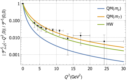
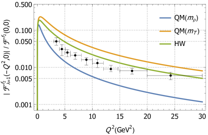
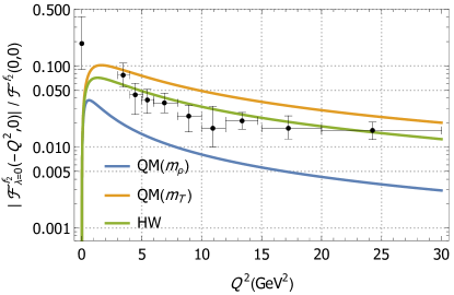
In Fig. 1 we show that also for the singly virtual TFF, for which data have been published by the Belle collaboration in [27], there is quite good agreement for the holographic hard-wall result for $\mathcal{F}^{T}_{1}$ ($\mathcal{F}^{T}_{3}$ does not contribute in the singly virtual case). For the normalized helicity-2 TFF, in particular for the lowest virtualities that have been measured, there is significantly better agreement than that obtained with the quark model [23] $\mathcal{F}^{T}_{1}$ with scale parameter $\Lambda_{T}$ set to either $m_{\rho}$ [25] or $M_{T}$ [29, 23]. This also holds true for the other helicities, although there the agreement at the lowest virtualities is not as good. Like the quark model, the holographic result fails to account for a nonvanishing helicity-0 contribution at zero virtuality as this would require a non-zero $\mathcal{F}^{T}_{2}$.

In Ref. [22], the Belle data have been fitted with a quark-model scale parameter of $\Lambda_{T}=1.222(66)$ GeV, slightly less than $m_{T}$. This implies a slope parameter of $2/1.222^{2}=1.34\,\mathrm{GeV}^{2}$. While the hQCD result provides a fit of roughly comparable quality, it involves a significantly larger slope parameter, $1.203/m_{\rho}^{2}=2.00\,\mathrm{GeV}^{2}$, half-way to the slope parameter $2/m_{\rho}^{2}=3.33\,\mathrm{GeV}^{2}$ obtained when $\Lambda_{T}$ is set to $m_{\rho}$ as advocated in [25].

Unfortunately, no experimental data for the doubly virtual case are available, which would test both $\mathcal{F}^{T}_{1}$ and $\mathcal{F}^{T}_{3}$. The doubly virtual TFFs enter in the one-loop process $T\to e^{+}e^{-}$, however only experimental upper limits exist at the moment for $f_{2}(1270)$ and $a_{2}(1320)$ [46].

IV.2 Asymptotic behavior

The asymptotic behavior of tensor FFT in the cases where one or both photon momenta are Euclidean and large, with respect of $\Lambda_{QCD}$, have been studied in Ref.[29], using the methods of light-cone expansion. Their results generalize those obtained for pseudoscalar meson TFF, in the symmetric limit [47, 48], and in the singly-virtual case (Brodsky-Lepage limit [49, 50, 51]) showing a milder asymptotic decrease compared to what would be obtained by VMD.

In [29], the following asymptotic behavior of the tensor meson TFF coefficients $\mathcal{F}^{T}_{i}$, written in terms of the average photon virtuality $Q$ and the asymmetry parameter $w$, has been obtained: With

$$Q^{2}=\frac{q_{1}^{2}+q_{2}^{2}}{2},\;\;w=\frac{q_{1}^{2}-q_{2}^{2}}{q_{1}^{2}+q_{2}^{2}}$$ (33)

the result obtained in [29] reads for $Q^{2}\to\infty$

$$\mathcal{F}_{1}^{T}(q_{1}^{2},q_{2}^{2}) \to\frac{4\sum_{a}C_{a}F_{T}^{a}m_{T}^{3}}{Q^{4}}f_{1}^{T}(w),$$

$$\mathcal{F}_{i}^{T}(q_{1}^{2},q_{2}^{2}) \to\frac{4\sum_{a}C_{a}F_{T}^{a}m_{T}^{5}}{Q^{6}}f_{i}^{T}(w),\qquad i\in\{2,3,4,5\},$$ (34)

with asymmetry functions

$$f^{T}_{1}(w) =\frac{5(1-w^{2})}{8w^{6}}\bigg{(}15-4w^{2}+\frac{3(5-3w^{2})}{2w}\ln\frac{1-w}{1+w}\bigg{)},$$

$$f^{T}_{2}(w) =-\frac{5}{8w^{6}}\bigg{(}15-13w^{2}+\frac{3(1-w^{2})(5-w^{2})}{2w}\ln\frac{1-w}{1+w}\bigg{)},$$

$$f^{T}_{3}(w) =-\frac{5}{8w^{6}}\bigg{(}15-w^{2}-\frac{w^{4}+6w^{2}-15}{2w}\ln\frac{1-w}{1+w}\bigg{)},$$

$$f^{T}_{4}(w) =-\frac{5}{24w^{6}}\bigg{(}45+30w-21w^{2}-8w^{3}+\frac{3(1+w)(15-5w-7w^{2}+w^{3})}{2w}\ln\frac{1-w}{1+w}\bigg{)},$$

$$f^{T}_{5}(w) =-\frac{5}{24w^{6}}\bigg{(}45-30w-21w^{2}+8w^{3}+\frac{3(1-w)(15+5w-7w^{2}-w^{3})}{2w}\ln\frac{1-w}{1+w}\bigg{)}.$$ (35)

The hQCD produces a $Q^{2}$ behavior in agreement with these results, however the asymmetry functions differ:

$$\mathcal{F}_{1} \to\frac{C_{T}m_{T}^{3}}{Q^{4}}\times\frac{-4}{w^{4}}\left(3-2w^{2}+\frac{3(1-w^{2})}{2w}\ln\frac{1-w}{1+w}\right)$$ (36)

$$\mathcal{F}_{3} \to\frac{C_{T}m_{T}^{5}}{Q^{6}}\times\frac{4}{w^{4}}\left(3+\frac{3-w^{2}}{2w}\ln\frac{1-w}{1+w}\right)$$ (37)

with

$$C_{T}=\frac{\text{tr}\mathcal{Q}^{2}}{8g_{5}^{2}J_{2}(m_{T}z_{0})}\frac{\sqrt{2/k_{T}}}{z_{0}}.$$ (38)

In (IV.2), $f^{T}_{1}(w)$ vanishes in the singly virtual limit $w\to\pm 1$, whereas the hQCD result has a finite value with $f^{T}_{1}(1)/f^{T}_{1}(0)=5/2$. On the other hand, both $f^{T}_{3}(w)$ functions have a minimum at $w=0$ and a logarithmic singularity for $w\to\pm 1$, with

$$\lim_{|w|\to 1}f^{T}_{3}(w)/f^{T}_{3}(0)=|\ln(1-|w|)|\times\begin{cases}\frac{105}{16}&\text{\cite[cite]{[\@@bibref{Number}{Hoferichter:2020lap}{}{}]}}\\ \frac{15}{4}&\text{hQCD}\end{cases}\;.$$ (39)

V Tensor meson contribution to $a_{\mu}^{HLbL}$

The tensor meson contribution to $a_{\mu}^{HLbL}$ has been evaluated in Ref. [24]  restricted, however, to the helicity-2 amplitude only, where $\mathcal{F}^{T}_{1}$ and $\mathcal{F}^{T}_{3}$ appear in the combination [29]

$$H_{+-;+2}=H_{-+;-2}\propto(\mathcal{F}^{T}_{1}+\frac{q_{1}^{2}q_{2}^{2}}{q_{1}\cdot q_{2}\,m_{T}^{2}}\mathcal{F}^{T}_{3}),$$ (40)

if the other structure functions are set to zero (here the different sign mentioned in footnote 2 does matter).

In the following, we shall provide a complete evaluation, first by employing the hQCD results for $\mathcal{F}^{T}_{1,3}$ in the formulae obtained in [28], which define the pole contribution of tensor mesons in the dispersive approach, and, second, by keeping all non-pole contribution as given by the hQCD result. In contrast to pseudoscalar and axial vector exchange contributions, where the two approaches lead to the same formulae, in the case of tensor mesons they are different (cf. Appendix A).

Furthermore, we consider two options: On the one hand, we take the hQCD model at face value, with one flavor-singlet tensor mode that is implemented just like a tensor glueball in top-down holographic models (for which radiative decays have been worked out recently in [52]), but which in the hard-wall model turns out to reproduce surprisingly well both mass and two-photon width of the dominant $f_{2}(1270)$ resonance. On the other hand, taking the hQCD results for the TFF, which reproduce quite well the singly virtual data for $f_{2}(1270)$ [27], as just a model for meson TFFs, we refit mass and two-photon width of the lowest tensor mode to exactly match the experimental values of the ground-state multiplet $f_{2}(1270)$, $a_{2}(1230$, and $f_{2}^{\prime}(1525)$.

Since the recent study of subleading HLBL contributions to $a_{\mu}$, which included tensor mesons, involves a matching to pQCD results with a separation scale of $Q_{0}=1.5$ GeV, we also present a break-up of the various contributions in an IR region defined by $Q_{i}\leq Q_{0}=1.5$ GeV, a UV region $Q_{i}>Q_{0}=1.5$ GeV for all $i$, and a mixed region for the remainder.

V.1 Pole contributions

Our results for the pole contribution as defined by the dispersive approach [28] are provided in Table 1.

$M_{T}$ [GeV]	$\Gamma_{\gamma\gamma}$ [keV]	IR	Mixed	UV	sum $[10^{-11}]$
1.235	2.46	$6.99-4.87=2.12$	$0.34-0.20=0.14$	$-0.001$	2.25
1.2754(8)	2.65(45)	$6.59-4.31=2.28$	$0.31-0.18=0.13$	$-0.0004$	2.40(41)
1.3182(6)	1.01(9)	$2.19-1.34=0.85$	$0.10-0.06=0.04$	$-0.0002$	0.89(8)
1.5173(24)	0.08(2)	$0.10-0.04=0.06$	$0.004-0.002=0.002$	0	0.06(2)
$f_{2}+a_{2}+f_{2}^{\prime}$		$8.87-5.69=3.18$	$0.42-0.25=0.17$	$-0.001$	3.35(42)

Table 1: $a_{\mu}$ results for the tensor meson contributions, in units of $10^{-11}$, obtained by inserting the hQCD results for $\mathcal{F}^{T}_{1,3}$ in the formulae obtained in [28] within the dispersive approach, where the first line corresponds to the lowest HW tensor mode normalized as in [26] and the remaining lines to a refit to experimental data. The IR region is defined by $Q_{i}\leq Q_{0}=1.5$ GeV, the UV region by $Q_{i}>Q_{0}=1.5$ GeV for all $i$. The first term of each sum is from $\overline{\Pi}_{1,2}$, while the second one is from the other 10 structure functions.

Similarly to [25], we observe large cancellations between contributions from the longitudinal pieces $\overline{\Pi}_{1,2}$ and the remaining $\overline{\Pi}_{i}$, however in contrast to [25], the net result is positive.

In Table 2, we show the pole contributions obtained by using the quark model TFF (12) with $\Lambda_{T}$ set to either $m_{\rho}$ as in [25] or $M_{T}$ as originally in [29, 23], and we compare to the hQCD result with only $\mathcal{F}^{T}_{1}$ (the latter also for $a_{2}$ and $f_{2}^{\prime}$). In this case the contributions from $\overline{\Pi}_{1,2}$ are reduced, the remaining ones increased, and the net result has a negative sign as in the quark model case. Compared to the holographic result where $\mathcal{F}^{T}_{3}$ is not left out, the absolute value is significantly larger.

	$M_{T}$ [GeV]	$\Gamma_{\gamma\gamma}$ [keV]	IR	Mixed	UV	sum $[10^{-11}]$
QM($m_{\rho}$)	1.2754(8)	2.65(45)	$1.94-3.84=-1.89$	$0.04-0.06=-0.02$	$-0.001$	$-1.91(32)$
QM($M_{T}$)	1.2754(8)	2.65(45)	$5.71-11.01=-5.30$	$0.64-0.86=-0.22$	$-0.001$	$-5.52(94)$
HW-$\mathcal{F}^{T}_{1}$ only	1.2754(8)	2.65(45)	$3.44-6.81=-3.37$	$0.15-0.22=-0.07$	$-0.002$	$-3.44(58)$
HW-$\mathcal{F}^{T}_{1}$ only	1.3182(6)	1.01(9)	$1.11-2.21=-1.10$	$0.05-0.07=-0.02$	$-0.0005$	$-1.12(10)$
HW-$\mathcal{F}^{T}_{1}$ only	1.5173	0.08(2)	$0.04-0.09=-0.04$	$0.002-0.003=-0.001$	0	$-0.045(10)$
HW-$\mathcal{F}^{T}_{1}$ only	$f_{2}+a_{2}+f_{2}^{\prime}$		$4.60-9.11=-4.51$	$0.20-0.29=-0.09$	$-0.003$	$-4.61(60)$

Table 2: $a_{\mu}$ results for the tensor meson contributions, in units of $10^{-11}$, obtained by inserting the quark model TFF for $\mathcal{F}^{T}_{1}$ ($\mathcal{F}^{T}_{2,3,4,5}=0$) in the formulae obtained in [28], with $\Lambda_{T}$ set to either $m_{\rho}$ [25] or $M_{T}$ [29, 23], compared to the HW result with only $\mathcal{F}^{T}_{1}$ (the latter also for $a_{2}$ and $f_{2}^{\prime}$).

V.2 Full holographic contributions

In Table 3, we compare result of the reduction to the pole contribution as defined in the optimized basis of [28] to the result obtained when the complete HLBL amplitude arising in hQCD from the exchange of tensor mesons is employed. The latter also involves the trace part of the metric fluctuations as well as their longitudinal components, corresponding to the fact that off-shell the Fierz-Pauli propagator is neither traceless nor transverse. This gives rise to extra tensor structures in the vertices, which in fact involve the same two basis tensors that appear in the case of scalar mesons (see Appendix A for the details).

The first line of Table 3 displays the difference for the ground-state tensor meson with model-given mass of 1.235 GeV. The contribution to $a_{\mu}$ is positive in both cases, but turns out to be more than twice as large in the full evaluation.

$M_{T}$ [GeV]	$\Gamma_{\gamma\gamma}$ [keV]	$a_{\mu}^{\mathrm{pole}}$ $[10^{-11}]$	$a_{\mu}^{\mathrm{full}}$ $[10^{-11}]$
1.235	2.46	7.33-5.07=2.26	9.15-3.27=5.88
2.262	0.60	2.01+0.64=2.65	1.08-0.21=0.87
3.280	1.91	0.80+0.34=1.14	0.36-0.09=0.27
4.295	0.75	0.30+0.15=0.45	0.11-0.03=0.08
5.310	1.75	0.16+0.09=0.25	0.04-0.01=0.03
[1.2–5.3]		10.60-3.84=6.76	10.75-3.62=7.13
[1.2–5.3]$|_{\mathrm{IR}}$		9.61-3.67=5.94	9.70-3.52=6.18

Table 3: Comparison of a full evaluation of the holographic results to the pole contribution as defined by the dispersive approach of Ref. [28], for the first five tensor modes. The first term of each sum is from $\overline{\Pi}_{1,2}$, while the second one is from the other 10 structure functions. The last line shows the amount of the summed contributions coming from the IR region defined by $Q_{i}\leq Q_{0}=1.5$ GeV.

Also shown are the $a_{\mu}$ contributions obtained by evaluating excited tensor modes. Even though the first excited tensor mode has a mass above 2 GeV and a rather small two-photon width, its $a_{\mu}$ contribution is even larger than the ground-state tensor when only the pole contribution is kept. By contrast, the full evaluation reduces this contribution strongly. Higher tensor modes give smaller contributions, but they fall comparatively slowly with mode number unless fully evaluated. The last line of Table 3 shows that the unnaturally large contributions from excited tensor mesons obtained in the pole-only formulae are appearing chiefly in the IR region.

Summing over the first five modes gives rather similar results, the difference being essentially in the attribution to the individual modes. In the full evaluation the lowest mode is already providing 95% of the total IR contribution, whereas in the case of the pole contribution this portion is only 38%.

The full holographic result for the tensor meson contribution is thus surprisingly large and positive, amounting to $a_{\mu}^{T}=5.9\times 10^{-11}$ ($5.4\times 10^{-11}$ from virtualities less than 1.5 GeV) When refitted to the parameters of $f_{2},a_{2},f_{2}^{\prime}$, an even larger result would be obtained, as Table 1 indicates, similar to the result of summing over the excited tensor modes as well (cf. Table 3).

Such a sizable positive contribution from the tensor mesons in place of the negative one obtained in [25] using the quark model might bring the total result for the HLBL contribution obtained in the dispersive approach [53] noticeably closer to the recent lattice results of Refs. [54, 55]. It would therefore be very desirable to be able to test the holographic prediction for the $T\to\gamma^{*}\gamma^{*}$ amplitude, away from the singly virtual limit.

Appendix A $\hat{\Pi}_{i}$ functions for $\mathcal{F}^{T}_{1,3}$ with and without non-pole terms

Let us briefly remind that the general analysis outlined in [9, 10], leads to the following master formula for the hadronic Light-by-Light contribution containing then only three integrals, which in terms of Euclidean momenta, takes the form:

$$a_{\mu}^{\mathrm{HLbL}} =\frac{2\alpha^{3}}{3\pi^{2}}\int_{0}^{\infty}dQ_{1}\int_{0}^{\infty}dQ_{2}\int_{-1}^{1}d\tau\sqrt{1-\tau^{2}}Q_{1}^{3}Q_{2}^{3}$$

$$\qquad\times\sum_{i=1}^{12}\bar{T}_{i}(Q_{1},Q_{2},\tau)\bar{\Pi}_{i}(Q_{1},Q_{2},\tau)\,,$$ (41)

where $Q_{1}$ and $Q_{2}$ are the radial components of the momenta. The hadronic scalar functions $\bar{\Pi}_{i}$ are evaluated for the reduced kinematics

$$(q_{1}^{2},q_{2}^{2},q_{3}^{2},q_{4}^{2})=(-Q_{1}^{2},-Q_{2}^{2},-Q_{1}^{2}-2Q_{1}Q_{2}\tau-Q_{2}^{2},0)\,.$$ (42)

(The complete list of the integral kernels $\bar{T}_{i}(Q_{1},Q_{2},\tau)$ can be found in Appendix B of [10].)

The twelve scalar function $\bar{\Pi}_{i}$, could in principle be obtained for any Hadronic Light-by Light tensor, i.e. the correlation function of four electromagnetic quark currents, obtained in any model provided it respects Lorentz and gauge invariance, crossing symmetries and some analyticity properties.

The extraction of the scalar functions $\bar{\Pi}_{i}$, is however a non trivial task, requiring the decomposition of the hadronic Light-by-Light tensor in particular basis of gauge invariant tensor structures.

This process produces certain ambiguities when one considers pole contributions to the HLbL tensor obtained by the exchange of single resonance, as is the case of the tensor resonances we are considering.

Only recently, a new optimized basis has been introduced in Ref.[28] and explicit non ambiguous formula have been found for the exchange of spin-1 and spin-2 resonances, in terms of their TFF and propagators. Actually, for tensor particle exchange, the formulas hold when the tensor TFF has simplified structures. Beyond the simplest case in which the only non vanishing coefficient is $\mathcal{F}_{1}$, as predicted by the Quark Model [23], unambiguous expressions in the dispersive framework for the $\bar{\Pi}_{i}$ can be written if either only $\mathcal{F}_{2,3}$ or $\mathcal{F}_{1,3}$ are non vanishing, the latter case precisely occurring in the hQCD model. We stress however that these ambiguities do not play a role in a full evaluation including non-pole terms. In that case any HLBL tensor gives rise to unambiguous $\bar{\Pi}_{i}(Q_{1},Q_{2},\tau)$. The data needed to define non-pole terms goes beyond the TFF where the meson is on-shell. As will be seen below, hQCD generates new Lorentz structures that are not present in the dispersive approach, since they do not contribute on-shell.

A.1 With non-pole terms

The full amplitude including trace terms of metric fluctuations reads

$$\mathcal{M}^{\mu\nu}_{\;\;\;\;\;\alpha\beta}(q_{1},q_{2})=(T_{1})^{\mu\nu}_{\;\;\;\;\;\alpha\beta}(-\frac{\text{tr}\mathcal{Q}^{2}}{g_{5}^{2}})\int\frac{dz}{z}h(z)\mathcal{J}(z,q_{1})\mathcal{J}(z,q_{2})$$

$$+(T_{3})^{\mu\nu}_{\;\;\;\;\;\alpha\beta}(-\frac{\text{tr}\mathcal{Q}^{2}}{g_{5}^{2}})\int\frac{dz}{z}h(z)\frac{\partial_{z}\mathcal{J}(z,q_{1})}{q_{1}^{2}}\frac{\partial_{z}\mathcal{J}(z,q_{2})}{q_{2}^{2}}$$

$$+\eta_{\alpha\beta}P^{\mu}_{\sigma}(q_{1})P^{\nu}_{\rho}(q_{2})\eta^{\sigma\rho}(\frac{\text{tr}\mathcal{Q}^{2}}{g_{5}^{2}})\int\frac{dz}{z}h(z)\partial_{z}\mathcal{J}(z,q_{1})\partial_{z}\mathcal{J}(z,q_{2})$$

$$+\frac{1}{2}\eta_{\alpha\beta}\left((q_{1})_{\sigma}P^{\mu}_{\rho}(q_{1})-(q_{1})_{\rho}P^{\mu}_{\sigma}(q_{1})\right)\left(q_{2}^{\sigma}P^{\nu\rho}(q_{2})-q_{2}^{\rho}P^{\nu\sigma}(q_{2})\right)$$

$$\times(\frac{\text{tr}\mathcal{Q}^{2}}{g_{5}^{2}})\int\frac{dz}{z}h(z)\mathcal{J}(z,q_{1})\mathcal{J}(z,q_{2}),$$ (43)

which can be concisely summarised as

$$\mathcal{M}^{\mu\nu}_{\;\;\;\;\;\alpha\beta}(q_{1},q_{2}) =\left((T^{T}_{1})^{\mu\nu}_{\;\;\;\;\;\alpha\beta}-(T_{1}^{S})^{\mu\nu}\eta_{\alpha\beta}\right)F_{1}(q_{1}^{2},q_{2}^{2})$$

$$+\left((T^{T}_{3})^{\mu\nu}_{\;\;\;\;\;\alpha\beta}-(T_{2}^{S})^{\mu\nu}\eta_{\alpha\beta}\right)F_{3}(q_{1}^{2},q_{2}^{2})$$ (44)

with $F_{1}=\frac{1}{m_{T}}\mathcal{F}_{1},\,F_{3}=\frac{1}{m_{T}^{3}}\mathcal{F}_{3}$ and using the Lorentz structures $(T_{i}^{S})^{\mu\nu}$ of [29] used in the scalar TFF. They are given by

$$(T_{1}^{S})^{\mu\nu} =q_{1}\cdot q_{2}\eta^{\mu\nu}-q_{2}^{\mu}q_{1}^{\nu}$$ (45)

$$(T_{2}^{S})^{\mu\nu} =q_{1}^{2}q_{2}^{2}\eta^{\mu\nu}+q_{1}\cdot q_{2}q_{1}^{\mu}q_{2}^{\nu}-q_{1}^{2}q_{2}^{\mu}q_{2}^{\nu}-q_{2}^{2}q_{1}^{\mu}q_{1}^{\nu}.$$ (46)

The full hQCD HLBL tensor is built up from two $\mathcal{M}$ vertices and one Fierz-Pauli propagator (6) and reads

$$\Pi^{\mu_{1}\mu_{2}\mu_{3}\mu_{4}}(q_{1},q_{2},q_{3},q_{4})=$$

$$i\mathcal{M}^{\mu_{1}\mu_{2}}_{\;\;\;\;\;\;\;\;\alpha\beta}(q_{1},q_{2})iG_{T}^{\alpha\beta\gamma\delta}(q_{1}+q_{2})i\mathcal{M}^{\mu_{3}\mu_{4}}_{\;\;\;\;\;\;\;\;\gamma\delta}(q_{3},q_{4})$$

$$+ i\mathcal{M}^{\mu_{1}\mu_{3}}_{\;\;\;\;\;\;\;\;\alpha\beta}(q_{1},q_{3})iG_{T}^{\alpha\beta\gamma\delta}(q_{1}+q_{3})i\mathcal{M}^{\mu_{2}\mu_{4}}_{\;\;\;\;\;\;\;\;\gamma\delta}(q_{2},q_{4})$$

$$+ i\mathcal{M}^{\mu_{1}\mu_{4}}_{\;\;\;\;\;\;\;\;\alpha\beta}(q_{1},q_{4})iG_{T}^{\alpha\beta\gamma\delta}(q_{1}+q_{4})i\mathcal{M}^{\mu_{2}\mu_{3}}_{\;\;\;\;\;\;\;\;\gamma\delta}(q_{2},q_{3}).$$ (47)

The Fierz-Pauli propagator is only traceless in $\alpha\beta$ on-shell; off-shell the trace is given by a contact term, which makes the trace terms above contribute to the longitudinal part of the $a_{\mu}$ contributions. Using the projection techniques of [9, 10, 28] one may calculate the relevant structure functions $\hat{\Pi}_{i}$ which can be straightforwardly used in the master formula for the $g-2$. They read:

$$\hat{\Pi}_{1}= \mathcal{F}_{1}(q_{2}^{2},0)\left(-\frac{2\mathcal{F}_{1}(q_{1}^{2},q_{3}^{2})}{m_{T}^{4}}+\frac{2q_{1}^{2}\mathcal{F}_{3}(q_{1}^{2},q_{3}^{2})}{m_{T}^{6}}\right)$$

$$+\mathcal{F}_{1}(q_{1}^{2},0)\left(-\frac{2\mathcal{F}_{1}(q_{2}^{2},q_{3}^{2})}{m_{T}^{4}}+\frac{2q_{2}^{2}\mathcal{F}_{3}(q_{2}^{2},q_{3}^{2})}{m_{T}^{6}}\right)$$

$$\hat{\Pi}_{4}= \frac{1}{3m_{T}^{8}}\mathcal{F}_{1}(q_{3}^{2},0)\left(2m_{T}^{2}q_{3}^{2}\mathcal{F}_{1}(q_{1}^{2},q_{2}^{2})-\left((q_{1}^{2}-q_{2}^{2})^{2}+(q_{1}^{2}+q_{2}^{2})q_{3}^{2}\right.\right.$$

$$\quad+\left.m_{T}^{2}\left(q_{1}^{2}+q_{2}^{2}+q_{3}^{2}\right)\right)\mathcal{F}_{3}(q_{1}^{2},q_{2}^{2})$$

$$+\frac{1}{3m_{T}^{8}(m_{T}^{2}-q_{3}^{2})}2\mathcal{F}_{1}(q_{3}^{2},0)\left(2m_{T}^{2}q_{3}^{2}(m_{T}^{2}+q_{3}^{2})\mathcal{F}_{1}(q_{1}^{2},q_{2}^{2})\right.$$

$$\quad+\left(2m_{T}^{4}(q_{1}^{2}+q_{2}^{2}+q_{3}^{2})-q_{3}^{2}\left((q_{1}^{2}-q_{2}^{2})^{2}+(q_{1}^{2}+q_{2}^{2})q_{3}^{2}\right)\right.$$

$$\quad-\left.m_{T}^{2}\left((q_{1}^{2}-q_{2}^{2})^{2}+2(q_{1}^{2}+q_{2}^{2})q_{3}^{2}+q_{3}^{4}\right)\right)\mathcal{F}_{3}(q_{1}^{2},q_{2}^{2})$$

$$+\frac{1}{m_{T}^{8}-m_{T}^{6}q_{2}^{2}}\mathcal{F}_{1}(q_{2}^{2},0)\left(m_{T}^{2}\left(-2m_{T}^{2}+q_{1}^{2}+q_{2}^{2}+q_{3}^{2}\right)\mathcal{F}_{1}(q_{1}^{2},q_{3}^{2})\right.$$

$$\quad-\left.\left(m_{T}^{2}(q_{1}^{2}-q_{2}^{2}-q_{3}^{2})+q_{3}^{2}(q_{1}^{2}+q_{2}^{2}+q_{3}^{2})\right)\mathcal{F}_{3}(q_{1}^{2},q_{3}^{2})\right)$$

$$+\frac{1}{m_{T}^{8}-m_{T}^{6}q_{1}^{2}}\mathcal{F}_{1}(q_{1}^{2},0)\left(m_{T}^{2}\left(-2m_{T}^{2}+q_{1}^{2}+q_{2}^{2}+q_{3}^{2}\right)\mathcal{F}_{1}(q_{2}^{2},q_{3}^{2})\right.$$

$$\quad+\left.\left(m_{T}^{2}(q_{1}^{2}-q_{2}^{2}+q_{3}^{2})-q_{3}^{2}(q_{1}^{2}+q_{2}^{2}+q_{3}^{2})\right)\mathcal{F}_{3}(q_{2}^{2},q_{3}^{2})\right)$$

$$\hat{\Pi}_{7}= -\frac{2(m_{T}^{2}-q_{1}^{2}+q_{2}^{2})\mathcal{F}_{1}(q_{3}^{2},0)\mathcal{F}_{3}(q_{1}^{2},q_{2}^{2})}{m_{T}^{8}-m_{T}^{6}q_{3}^{2}}$$

$$+\frac{\mathcal{F}_{1}(q_{2}^{2},0)\left(-2m_{T}^{2}\mathcal{F}_{1}(q_{1}^{2},q_{3}^{2})+2(m_{T}^{2}+q_{3}^{2})\mathcal{F}_{3}(q_{1}^{2},q_{3}^{2})\right)}{m_{T}^{8}-m_{T}^{6}q_{2}^{2}}$$

$$-\frac{2\mathcal{F}_{1}(q_{1}^{2},0)\mathcal{F}_{3}(q_{2}^{2},q_{3}^{2})}{m_{T}^{6}-m_{T}^{4}q_{1}^{2}}.$$

$$\hat{\Pi}_{17}= -\frac{1}{3m_{T}^{8}}\Bigg{(}\frac{2m_{T}^{2}(3m_{T}^{2}+2q_{3}^{2})\mathcal{F}_{1}(q_{1}^{2},q_{2}^{2})\mathcal{F}_{1}(q_{3}^{2},0)}{m_{T}^{2}-q_{3}^{2}}$$

$$\quad-\frac{1}{m_{T}^{2}-q_{3}^{2}}\left(3m_{T}^{2}(q_{1}^{2}+q_{2}^{2})+2(m_{T}^{2}+q_{1}^{2}+q_{2}^{2})q_{3}^{2}\right)\mathcal{F}_{1}(q_{3}^{2},0)\mathcal{F}_{3}(q_{1}^{2},q_{2}^{2})$$

$$\quad+3m_{T}^{2}\left(\frac{(q_{1}^{2}-q_{3}^{2})\mathcal{F}_{1}(q_{2}^{2},0)\mathcal{F}_{3}(q_{1}^{2},q_{3}^{2})}{m_{T}^{2}-q_{2}^{2}}+\frac{(q_{2}^{2}-q_{3}^{2})\mathcal{F}_{1}(q_{1}^{2},0)\mathcal{F}_{3}(q_{2}^{2},q_{3}^{2})}{m_{T}^{2}-q_{1}^{2}}\right)\Bigg{)}.$$

$$\hat{\Pi}_{39}= \frac{\mathcal{F}_{1}(q_{3}^{2},0)\left(2m_{T}^{2}\mathcal{F}_{1}(q_{1}^{2},q_{2}^{2})+\left(2m_{T}^{2}-q_{1}^{2}-q_{2}^{2}\right)\mathcal{F}_{3}(q_{1}^{2},q_{2}^{2})\right)}{m_{T}^{8}-m_{T}^{6}q_{3}^{2}}$$

$$+\frac{\mathcal{F}_{1}(q_{2}^{2},0)\left(2m_{T}^{2}\mathcal{F}_{1}(q_{1}^{2},q_{3}^{2})+\left(2m_{T}^{2}-q_{1}^{2}-q_{3}^{2}\right)\mathcal{F}_{3}(q_{1}^{2},q_{3}^{2})\right)}{m_{T}^{8}-m_{T}^{6}q_{2}^{2}}$$

$$+\frac{\mathcal{F}_{1}(q_{1}^{2},0)\left(2m_{T}^{2}\mathcal{F}_{1}(q_{2}^{2},q_{3}^{2})+\left(2m_{T}^{2}-q_{2}^{2}-q_{3}^{2}\right)\mathcal{F}_{3}(q_{2}^{2},q_{3}^{2})\right)}{m_{T}^{8}-m_{T}^{6}q_{1}^{2}}.$$

$$\hat{\Pi}_{54}= \frac{(q_{1}^{2}-q_{2}^{2})\mathcal{F}_{1}(q_{3}^{2},0)\mathcal{F}_{3}(q_{1}^{2},q_{2}^{2})}{m_{T}^{6}\left(m_{T}^{2}-q_{3}^{2}\right)}$$

$$+\frac{\mathcal{F}_{1}(q_{2}^{2},0)\left(2m_{T}^{2}\mathcal{F}_{1}(q_{1}^{2},q_{3}^{2})-q_{1}^{2}\mathcal{F}_{3}(q_{1}^{2},q_{3}^{2})-q_{3}^{2}\mathcal{F}_{3}(q_{1}^{2},q_{3}^{2})\right)}{m_{T}^{6}\left(m_{T}^{2}-q_{2}^{2}\right)}$$

$$-\frac{\mathcal{F}_{1}(q_{1}^{2},0)\left(2m_{T}^{2}\mathcal{F}_{1}(q_{2}^{2},q_{3}^{2})-q_{2}^{2}\mathcal{F}_{3}(q_{2}^{2},q_{3}^{2})-q_{3}^{2}\mathcal{F}_{3}(q_{2}^{2},q_{3}^{2})\right)}{m_{T}^{6}\left(m_{T}^{2}-q_{1}^{2}\right)}.$$ (48)

A.2 Pole terms only

For the sake of comparison, we also include below the pole-term parts as defined by the dispersive procedure in the optimized basis of Ref. [28].

$$\hat{\Pi}_{1}=\mathcal{F}_{1}(q_{2}^{2},0)\left(-\frac{\mathcal{F}_{1}(q_{1}^{2},q_{3}^{2})}{m_{T}^{4}}+\frac{(-m_{T}^{2}+q_{1}^{2})\mathcal{F}_{3}(q_{1}^{2},q_{3}^{2})}{m_{T}^{6}}\right) +$$

$$\mathcal{F}_{1}(q_{1}^{2},0)\left(-\frac{\mathcal{F}_{1}(q_{2}^{2},q_{3}^{2})}{m_{T}^{4}}+\frac{(-m_{T}^{2}+q_{2}^{2})\mathcal{F}_{3}(q_{2}^{2},q_{3}^{2})}{m_{T}^{6}}\right)$$

$$\hat{\Pi}_{4}= \frac{1}{3m_{T}^{8}(m_{T}^{2}-q_{3}^{2})}\mathcal{F}_{1}(q_{3}^{2},0)\Bigg{(}8m_{T}^{4}q_{3}^{2}\mathcal{F}_{1}(q_{1}^{2},q_{2}^{2})+$$

$$\left(6m_{T}^{6}-3m_{T}^{2}(q_{1}^{2}-q_{2}^{2})^{2}+3m_{T}^{4}(q_{1}^{2}+q_{2}^{2})-\right.$$

$$\left(4m_{T}^{4}+(q_{1}^{2}-q_{2}^{2})^{2}+5m_{T}^{2}(q_{1}^{2}+q_{2}^{2})\right)q_{3}^{2}\Bigg{)}\mathcal{F}_{3}(q_{1}^{2},q_{2}^{2})\Bigg{)}+$$

$$\frac{1}{m_{T}^{8}-m_{T}^{6}q_{2}^{2}} \mathcal{F}_{1}(q_{2}^{2},0)\Bigg{(}m_{T}^{2}(-4m_{T}^{2}+q_{1}^{2}+3q_{2}^{2}+q_{3}^{2})\mathcal{F}_{1}(q_{1}^{2},q_{3}^{2})+$$

$$\left(m_{T}^{4}-q_{1}^{2}q_{2}^{2}+2m_{T}^{2}q_{3}^{2}-q_{3}^{2}(q_{1}^{2}+2q_{2}^{2}+q_{3}^{2})\right)\mathcal{F}_{3}(q_{1}^{2},q_{3}^{2})\Bigg{)}+$$

$$\frac{1}{m_{T}^{8}-m_{T}^{6}q_{1}^{2}} \mathcal{F}_{1}(q_{1}^{2},0)\Bigg{(}m_{T}^{2}(-4m_{T}^{2}+3q_{1}^{2}+q_{2}^{2}+q_{3}^{2})\mathcal{F}_{1}(q_{2}^{2},q_{3}^{2})+$$

$$\left(m_{T}^{4}-q_{1}^{2}q_{2}^{2}+2m_{T}^{2}q_{3}^{2}-q_{3}^{2}(2q_{1}^{2}+q_{2}^{2}+q_{3}^{2})\right)\mathcal{F}_{3}(q_{2}^{2},q_{3}^{2})\Bigg{)}$$

$$\hat{\Pi}_{7}= -\frac{2(m_{T}^{2}-q_{1}^{2}+q_{2}^{2})\mathcal{F}_{1}(q_{3}^{2},0)\mathcal{F}_{3}(q_{1}^{2},q_{2}^{2})}{m_{T}^{8}-m_{T}^{6}q_{3}^{2}}+$$

$$\frac{\mathcal{F}_{1}(q_{2}^{2},0)\left(-2m_{T}^{2}\mathcal{F}_{1}(q_{1}^{2},q_{3}^{2})+2(m_{T}^{2}+q_{3}^{2})\mathcal{F}_{3}(q_{1}^{2},q_{3}^{2})\right)}{m_{T}^{8}-m_{T}^{6}q_{2}^{2}}-$$

$$\frac{\mathcal{F}_{1}(q_{1}^{2},0)\left(2m_{T}^{2}\mathcal{F}_{3}(q_{2}^{2},q_{3}^{2})\right)}{m_{T}^{8}-m_{T}^{6}q_{1}^{2}}$$

$$\hat{\Pi}_{17}= \frac{1}{3m_{T}^{8}(m_{T}^{2}-q_{3}^{2})}\mathcal{F}_{1}(q_{3}^{2},0)\Big{(}-2(3m_{T}^{4}+2m_{T}^{2}q_{3}^{2})\mathcal{F}_{1}(q_{1}^{2},q_{2}^{2})$$

$$\quad+\left(3m_{T}^{2}(q_{1}^{2}+q_{2}^{2})+2(m_{T}^{2}+q_{1}^{2}+q_{2}^{2})q_{3}^{2}\right)\mathcal{F}_{3}(q_{1}^{2},q_{2}^{2})\Big{)}$$

$$+\frac{(-q_{1}^{2}+q_{3}^{2})\mathcal{F}_{1}(q_{2}^{2},0)\mathcal{F}_{3}(q_{1}^{2},q_{3}^{2})}{m_{T}^{8}-m_{T}^{6}q_{2}^{2}}$$

$$+\frac{(-q_{2}^{2}+q_{3}^{2})\mathcal{F}_{1}(q_{1}^{2},0)\mathcal{F}_{3}(q_{2}^{2},q_{3}^{2})}{m_{T}^{8}-m_{T}^{6}q_{1}^{2}}$$

$$\hat{\Pi}_{39}= \frac{\mathcal{F}_{1}(q_{3}^{2},0)\left(4m_{T}^{2}\mathcal{F}_{1}(q_{1}^{2},q_{2}^{2})+\left(4m_{T}^{2}-2(q_{1}^{2}+q_{2}^{2})\right)\mathcal{F}_{3}(q_{1}^{2},q_{2}^{2})\right)}{2m_{T}^{6}(m_{T}^{2}-q_{3}^{2})}$$

$$+\frac{\mathcal{F}_{1}(q_{2}^{2},0)\left(4m_{T}^{2}\mathcal{F}_{1}(q_{1}^{2},q_{3}^{2})+\left(4m_{T}^{2}-2(q_{1}^{2}+q_{3}^{2})\right)\mathcal{F}_{3}(q_{1}^{2},q_{3}^{2})\right)}{2m_{T}^{6}(m_{T}^{2}-q_{2}^{2})}$$

$$+\frac{\mathcal{F}_{1}(q_{1}^{2},0)\left(4m_{T}^{2}\mathcal{F}_{1}(q_{2}^{2},q_{3}^{2})+\left(4m_{T}^{2}-2(q_{2}^{2}+q_{3}^{2})\right)\mathcal{F}_{3}(q_{2}^{2},q_{3}^{2})\right)}{2m_{T}^{6}(m_{T}^{2}-q_{1}^{2})}$$

$$\hat{\Pi}_{54}= \frac{(q_{1}^{2}-q_{2}^{2})\mathcal{F}_{1}(q_{3}^{2},0)\mathcal{F}_{3}(q_{1}^{2},q_{2}^{2})}{m_{T}^{8}-m_{T}^{6}q_{3}^{2}}$$

$$+\frac{\mathcal{F}_{1}(q_{2}^{2},0)\left(2m_{T}^{2}\mathcal{F}_{1}(q_{1}^{2},q_{3}^{2})-(q_{1}^{2}+q_{3}^{2})\mathcal{F}_{3}(q_{1}^{2},q_{3}^{2})\right)}{m_{T}^{8}-m_{T}^{6}q_{2}^{2}}$$

$$+\frac{\mathcal{F}_{1}(q_{1}^{2},0)\left(-2m_{T}^{2}\mathcal{F}_{1}(q_{2}^{2},q_{3}^{2})+(q_{2}^{2}+q_{3}^{2})\mathcal{F}_{3}(q_{2}^{2},q_{3}^{2})\right)}{m_{T}^{8}-m_{T}^{6}q_{1}^{2}}$$ (49)

References

- [1] T. Aoyama et al., The anomalous magnetic moment of the muon in the Standard Model, Phys. Rept. 887 (2020) 1 [2006.04822].
- [2] K. Melnikov and A. Vainshtein, Hadronic light-by-light scattering contribution to the muon anomalous magnetic moment revisited, Phys. Rev. D70 (2004) 113006 [hep-ph/0312226].
- [3] J. Bijnens, N. Hermansson-Truedsson, L. Laub and A. Rodríguez-Sánchez, Short-distance HLbL contributions to the muon anomalous magnetic moment beyond perturbation theory, JHEP 10 (2020) 203 [2008.13487].
- [4] J. Bijnens, N. Hermansson-Truedsson, L. Laub and A. Rodríguez-Sánchez, The two-loop perturbative correction to the HLbL at short distances, JHEP 04 (2021) 240 [2101.09169].
- [5] J. Bijnens, N. Hermansson-Truedsson and A. Rodríguez-Sánchez, Constraints on the hadronic light-by-light in the Melnikov-Vainshtein regime, 2211.17183.
- [6] J. Bijnens, N. Hermansson-Truedsson and A. Rodríguez-Sánchez, Constraints on the hadronic light-by-light in corner kinematics for the muon , 2411.09578.
- [7] G. Colangelo, M. Hoferichter, M. Procura and P. Stoffer, Dispersive approach to hadronic light-by-light scattering, JHEP 09 (2014) 091 [1402.7081].
- [8] G. Colangelo, M. Hoferichter, B. Kubis, M. Procura and P. Stoffer, Towards a data-driven analysis of hadronic light-by-light scattering, Phys. Lett. B738 (2014) 6 [1408.2517].
- [9] G. Colangelo, M. Hoferichter, M. Procura and P. Stoffer, Dispersion relation for hadronic light-by-light scattering: theoretical foundations, JHEP 09 (2015) 074 [1506.01386].
- [10] G. Colangelo, M. Hoferichter, M. Procura and P. Stoffer, Dispersion relation for hadronic light-by-light scattering: two-pion contributions, JHEP 04 (2017) 161 [1702.07347].
- [11] G. Eichmann, C.S. Fischer, E. Weil and R. Williams, Single pseudoscalar meson pole and pion box contributions to the anomalous magnetic moment of the muon, Phys. Lett. B797 (2019) 134855 [1903.10844].
- [12] G. Eichmann, C.S. Fischer and R. Williams, Kaon-box contribution to the anomalous magnetic moment of the muon, Phys. Rev. D101 (2020) 054015 [1910.06795].
- [13] G. Eichmann, C.S. Fischer, T. Haeuser and O. Regenfelder, Axial-vector and scalar contributions to hadronic light-by-light scattering, 2411.05652.
- [14] P. Roig, A. Guevara and G. López Castro, form factors in resonance chiral theory and the light-by-light contribution to the muon , Phys. Rev. D89 (2014) 073016 [1401.4099].
- [15] A. Guevara, P. Roig and J.J. Sanz-Cillero, Pseudoscalar pole light-by-light contributions to the muon in Resonance Chiral Theory, JHEP 06 (2018) 160 [1803.08099].
- [16] E.J. Estrada, S. Gonzàlez-Solís, A. Guevara and P. Roig, Improved transition form factors in resonance chiral theory and their contribution, 2409.10503.
- [17] J. Leutgeb and A. Rebhan, Axial vector transition form factors in holographic QCD and their contribution to the anomalous magnetic moment of the muon, Phys. Rev. D 101 (2020) 114015 [1912.01596].
- [18] L. Cappiello, O. Catà, G. D’Ambrosio, D. Greynat and A. Iyer, Axial-vector and pseudoscalar mesons in the hadronic light-by-light contribution to the muon , Phys. Rev. D 102 (2020) 016009 [1912.02779].
- [19] J. Leutgeb and A. Rebhan, Hadronic light-by-light contribution to the muon g-2 from holographic QCD with massive pions, Phys. Rev. D 104 (2021) 094017 [2108.12345].
- [20] J. Leutgeb, J. Mager and A. Rebhan, Hadronic light-by-light contribution to the muon from holographic QCD with solved problem, Phys. Rev. D 107 (2023) 054021 [2211.16562].
- [21] J. Leutgeb, J. Mager and A. Rebhan, Superconnections in AdS/QCD and the hadronic light-by-light contribution to the muon , 2411.10432.
- [22] I. Danilkin and M. Vanderhaeghen, Light-by-light scattering sum rules in light of new data, Phys. Rev. D95 (2017) 014019 [1611.04646].
- [23] G.A. Schuler, F.A. Berends and R. van Gulik, Meson photon transition form-factors and resonance cross-sections in collisions, Nucl. Phys. B 523 (1998) 423 [hep-ph/9710462].
- [24] P. Colangelo, F. Giannuzzi and S. Nicotri, Hadronic light-by-light scattering contributions to from axial-vector and tensor mesons in the holographic soft-wall model, Phys. Rev. D 109 (2024) 094036 [2402.07579].
- [25] M. Hoferichter, P. Stoffer and M. Zillinger, Dispersion relation for hadronic light-by-light scattering: subleading contributions, 2412.00178.
- [26] E. Katz, A. Lewandowski and M.D. Schwartz, Tensor mesons in AdS/QCD, Phys. Rev. D 74 (2006) 086004 [hep-ph/0510388].
- [27] Belle collaboration, Study of pair production in single-tag two-photon collisions, Phys. Rev. D 93 (2016) 032003 [1508.06757].
- [28] M. Hoferichter, P. Stoffer and M. Zillinger, An optimized basis for hadronic light-by-light scattering, JHEP 04 (2024) 092 [2402.14060].
- [29] M. Hoferichter and P. Stoffer, Asymptotic behavior of meson transition form factors, JHEP 05 (2020) 159 [2004.06127].
- [30] M. Poppe, Exclusive Hadron Production in Two Photon Reactions, Int. J. Mod. Phys. A 1 (1986) 545.
- [31] W.A. Bardeen and W.K. Tung, Invariant amplitudes for photon processes, Phys. Rev. 173 (1968) 1423.
- [32] R. Tarrach, Invariant Amplitudes for Virtual Compton Scattering Off Polarized Nucleons Free from Kinematical Singularities, Zeros and Constraints, Nuovo Cim. A28 (1975) 409.
- [33] T. Sakai and S. Sugimoto, Low energy hadron physics in holographic QCD, Prog.Theor.Phys. 113 (2005) 843 [hep-th/0412141].
- [34] J. Erlich, E. Katz, D.T. Son and M.A. Stephanov, QCD and a holographic model of hadrons, Phys. Rev. Lett. 95 (2005) 261602 [hep-ph/0501128].
- [35] L. Da Rold and A. Pomarol, Chiral symmetry breaking from five-dimensional spaces, Nucl. Phys. B721 (2005) 79 [hep-ph/0501218].
- [36] J. Hirn and V. Sanz, Interpolating between low and high energy QCD via a 5-D Yang-Mills model, JHEP 12 (2005) 030 [hep-ph/0507049].
- [37] A. Karch, E. Katz, D.T. Son and M.A. Stephanov, Linear confinement and AdS/QCD, Phys. Rev. D74 (2006) 015005 [hep-ph/0602229].
- [38] J.M. Maldacena, The Large N limit of superconformal field theories and supergravity, Int.J.Theor.Phys. 38 (1999) 1113 [hep-th/9711200].
- [39] S.S. Gubser, I.R. Klebanov and A.M. Polyakov, Gauge theory correlators from noncritical string theory, Phys. Lett. B 428 (1998) 105 [hep-th/9802109].
- [40] E. Witten, Anti-de Sitter space and holography, Adv. Theor. Math. Phys. 2 (1998) 253 [hep-th/9802150].
- [41] V.A. Novikov, M.A. Shifman, A.I. Vainshtein and V.I. Zakharov, Are All Hadrons Alike? , Nucl. Phys. B 191 (1981) 301.
- [42] S. Mamedov, Z. Hashimli and S. Jafarzade, Tensor meson couplings in AdS/QCD, Phys. Rev. D 108 (2023) 114032 [2308.12392].
- [43] JPAC collaboration, Exclusive tensor meson photoproduction, Phys. Rev. D 102 (2020) 014003 [2005.01617].
- [44] L.D. Landau, On the angular momentum of a system of two photons, Dokl. Akad. Nauk Ser. Fiz. 60 (1948) 207.
- [45] C.-N. Yang, Selection Rules for the Dematerialization of a Particle Into Two Photons, Phys. Rev. 77 (1950) 242.
- [46] M.N. Achasov et al., Search for direct production of and mesons in annihilation, Phys. Lett. B 492 (2000) 8 [hep-ex/0009048].
- [47] V.A. Nesterenko and A.V. Radyushkin, Comparison of the QCD Sum Rule Approach and Perturbative QCD Analysis for Process, Sov. J. Nucl. Phys. 38 (1983) 284.
- [48] V.A. Novikov, M.A. Shifman, A.I. Vainshtein, M.B. Voloshin and V.I. Zakharov, Use and Misuse of QCD Sum Rules, Factorization and Related Topics, Nucl. Phys. B237 (1984) 525.
- [49] G.P. Lepage and S.J. Brodsky, Exclusive Processes in Quantum Chromodynamics: Evolution Equations for Hadronic Wave Functions and the Form-Factors of Mesons, Phys. Lett. 87B (1979) 359.
- [50] G.P. Lepage and S.J. Brodsky, Exclusive Processes in Perturbative Quantum Chromodynamics, Phys. Rev. D22 (1980) 2157.
- [51] S.J. Brodsky and G.P. Lepage, Large Angle Two Photon Exclusive Channels in Quantum Chromodynamics, Phys. Rev. D24 (1981) 1808.
- [52] F. Hechenberger, J. Leutgeb and A. Rebhan, Radiative meson and glueball decays in the Witten-Sakai-Sugimoto model, Phys. Rev. D 107 (2023) 114020 [2302.13379].
- [53] M. Hoferichter, P. Stoffer and M. Zillinger, A complete dispersive evaluation of hadronic light-by-light scattering, 2412.00190.
- [54] T. Blum, N. Christ, M. Hayakawa, T. Izubuchi, L. Jin, C. Jung et al., Hadronic light-by-light contribution to the muon anomaly from lattice QCD with infinite volume QED at physical pion mass, 2304.04423.
- [55] Z. Fodor, A. Gerardin, L. Lellouch, K.K. Szabo, B.C. Toth and C. Zimmermann, Hadronic light-by-light scattering contribution to the anomalous magnetic moment of the muon at the physical pion mass, 2411.11719.