Testing Born’s rule via photoionization of helium
Abstract
It is shown how state-of-the-art attosecond photoionization experiments can test Born’s rule – a postulate of quantum mechanics – via the so-called Sorkin test. A simulation of the Sorkin test under consideration of typical experimental noise and data acquisition efficiencies infers an achievable measurement precision in the range of the best Sorkin tests to date. The implementation of further fundamental tests of quantum mechanics is discussed.
Attosecond physics emerged around the beginning of this millennium, from the desire to resolve electronic dynamics in matter on short time scales [1, 2]. It encompasses the ionization of atoms [3, 4, 5, 6], molecules [7, 8], and solids [9], typically through the exposure to short, extreme-ultraviolet (XUV) light pulses, often synchronized with infrared (IR) probe pulses to analyze the induced photoionization dynamics [10, 11, 12, 13, 14, 15, 16, 17]. The ever-increasing stability and controllability of available light sources promises the synergy of attosecond physics and quantum information science [18, 19]. First steps approach the exploration of entanglement in double photoionization [20, 21, 22], electron-ion entanglement [23, 24, 16, 17] or the driving of high-harmonic generation via non-classical light fields [25, 26, 27], while implementations of quantum information processing and fundamental tests of quantum theory have not been achieved yet in these rather complex settings of light-matter interaction.
Testing the foundations of quantum mechanics is tantamount to testing the postulates [28] on which quantum theory is build upon. Since no quantum mechanical prediction has so far been violated within the limits of experimental precision, there is no evidence against the validity of these postulates. Revealing the limits of quantum theory therefore requires, if at all, highly precise experiments, ideally targeted to test specific postulates in all possible physical system. One of these postulates is Born’s rule [29]. It establishes the connection between the mathematical formalism and the experimentally recorded counting statistics by stating that event probabilities are given by the squared modulus of the associated transition amplitudes. Since Born’s rule implies the restriction of quantum interference to pairs of paths [29], three- or multi-path interferometers specifically allow to asses the validity of Born’s rule via the so-called Sorkin test [30], and to rule out alternative theories [31, 32]. However, none of the hitherto implemented Sorkin tests using single photons [33, 34, 35, 36, 37, 38], nuclear magnetic resonance in a spin ensemble [39], a single nitrogen-vacancy center in diamond [40], atomic matter waves [41], single dye molecules [42], two-photon interference [43], and coherent light together with homodyne detection [44] (see [45] for an overview) found evidence against the validity of Born’s rule. To further assess the validity and accuracy of Born’s rule therefore calls for an increased precision in these experiments, as well as an expansion of the Sorkin test to physical systems that have not been considered yet for its implementation.
Here, we propose an implementation of the Sorkin test in the photoionization process of helium. We show how spectral shaping of the IR probe pulse in typical pump-probe photoionization experiments allows the realization of three-path interferometers. We perform a Monte Carlo simulation of the Sorkin test in consideration of typical noise sources in state-of-the-art experiments, and infer an achievable precision of , i.e., at the same level as most Sorkin tests to date [39, 37, 40, 46]. The interferometer’s intrinsic phase stability makes attosecond photoionization also a promising candidate for further tests of quantum mechanics, such as the so-called Peres test [47], which we briefly discuss at the end of this contribution. As a result, we establish the potential of attosecond photoionization as a platform for fundamental tests of quantum mechanics.
Sorkin test – Given a quantum system described by the state in a Hilbert space , Born’s rule [29] states that the measurement of an observable on , with eigenstates and corresponding eigenvalues , yields the outcome with probability . As a direct consequence, for superpositions of distinct components and , with , such as in a double-slit experiment, it entails the interference of the transition amplitudes and : The probability to observe the outcome depends not only on the probabilities corresponding to the individual components , but also on the interference term , which is sensitive to the relative phase between and . By adding a third component, , the classical additivity of the individual probabilities , , is merely accompanied by interference terms between pairs of amplitudes, and no additional interference term between more than two transition amplitudes intervenes. Consequently, following the idea of Sorkin [30], we can define such an additional interference term as the deviation from the quantum mechanical prediction for [33], which can be expressed in terms of measurable probabilities alone, , and must vanish if Born’s rule applies. In order to correct for constant background signals in experiments, one usually subtracts the detection signal in the absence of all components from each probability , with , i.e., , yielding the corrected interference terms and [33, 34, 39, 37, 48, 45], which constitute the so-called Sorkin parameter [33]
| (1) |
It defines a quantitative measure of potential deviations [30] from Born’s rule, experimentally accessible by recording all the probabilities , .
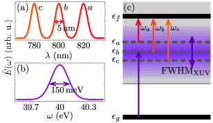
Photoionization model – As we show in the following, state-of-the-art experiments on the photoionization of atoms via short multi-chromatic laser pulses [12, 49, 50, 24, 17, 51] realize stable multi-path interference, which serves well for high-precision measurements of the Sorkin parameter (1). To this end, consider single-electron, laser-assisted photoionization [52] into the structureless continuum of helium atoms, induced by a broadband extreme ultraviolet (XUV) pump pulse, with central frequency and spectral width , as well as a synchronized infrared (IR) probe pulse, composed of three spectral components with central frequencies , such that , and equal, narrow spectral widths [see Figs. 1(a,b)]. Note that, in contrast to typical pump-probe spectroscopy schemes [10], here the time delays between the th IR component and the XUV pump pulse are ideally kept constant during the measurement. The absorption of a photon from the XUV pulse induces a transition from the electron’s bound ground state to an intermediate continuum state with broad energy distribution (as naturally provided via femto- or attosecond laser pulses) that has significant overlap with three distinct continuum states corresponding to the energies , where is the photoelectron’s final state, interrogated by the experimental setup [see Fig. 1(c)]. Consequently, the subsequent absorption of a photon from either one of the spectrally narrow components of the IR pulse feeds the final energy state by three transition amplitudes, thus realizing a three-path interferometer.
Different path-configurations can be realized through the selection of subsets of the three available IR components , such that the corresponding probability to detect a photoelectron with energy yields . For example, is obtained in the presence of the IR components and , and in the absence of component . In this way, one has access to all probabilities which enter Eq. (1).
Theoretical description – To specify the probability , with amplitude , we follow Ref. [53] and derive an explicit expression for the individual transition amplitudes (see [54] for details): Due to the injected light fields’ intensities and their large wavelengths as compared to the electronic initial state’s scale, we can treat the laser fields classically and describe the light-matter interaction in dipole approximation, with the Hamiltonian [55], where is the field-free atomic component, and the interaction term, with the dipole operator and the total (phase stable) driving field, composed of the XUV pump and the IR spectral components , for all . In the weak coupling regime and in the absence of intermediate atomic resonances, the interaction term can be treated as a perturbation, with the perturbation order corresponding to the number of photons involved in the ionization process [55]. For initial interaction times and measurement times , the amplitude can be expanded to second order as
| (2) | ||||
with the interaction Hamiltonian in the interaction picture with respect to . By restricting ourselves to final energies , with , in a featureless continuum [see Fig. 1(c)], any single-photon absorption process becomes off-resonant, such that the first order term in (2) vanishes. The first non-vanishing term in (2) is thus of second order. It includes all four time-ordered combinations of two-photon processes (XUVIR, IRXUV, XUVXUV, and IRIR). However, only the absorption of a XUV photon followed by the absorption of an IR photon contributes, since both transitions XUVXUV and IRIR are highly off-resonant, and the IRXUV transition is highly unlikely as compared to the reverse time ordered one due to the absence of resonant intermediate states. Any three-photon process is also off-resonant, and, thus, suppressed. The first neglected, non-suppressed term is thus of fourth order. The transition amplitudes , , can therefore be written as [53, 54]
| (3) | ||||
with , and and the electric XUV and IR field in the frequency representation, respectively. Note that the neglected non-vanishing higher-order terms can give rise to a non-vanishing Sorkin parameter without a violation of Born’s rule, similar as in optical three-path experiments [56, 57, 36, 58].
As illustrated in Figs. 1(a,b), we model the pump and probe fields by Gaussian pulses and , with central frequencies and , respectively, and spectral widths and . Since the helium target exhibits a featureless continuum between the single ionization threshold and doubly excited states at energies around [59, 60], addressed by the here employed driving frequencies, the intermediate and final states are featureless continuum states for which we can employ the so-called on-shell approximation [53].
In general, there can be multiple ionization channels [61, 62], such that photoelectrons with final energy can have different angular momentum states. For two-photon absorption in helium, the dipole selection rules allow the transition from the ground state over a intermediate state to either an or a final state. For the measurement of the Sorkin parameter (1), these angular momentum states, however, need not be resolved, allowing for angle-integrated measurements. In order to make this explicit, consider the photoelectron’s continuum basis states , with energy , angular momentum quantum number , and magnetic quantum number . The photoelectron’s state after two-photon absorption can then be written as , with coefficients . By the orthogonality of the angular momentum states, i.e., , the probability to find the photoelectron in the final energy decomposes as , with . Together with the linearity of the interference term with respect to [see above Eq. (1)], we see that the photoelectron’s angular momentum states have no effect on the vanishing of the Sorkin parameter (1).
Simulation – With the help of Eq. (3) (see [54] for details), we numerically simulate the Sorkin test and estimate the achievable precision of the Sorkin parameter (1) under typical experimental conditions for final energies in the energie window of width around , specified by , with . To this end, we conservatively estimate the most dominant sources of noise in typical state-of-the-art experiments. For the field amplitudes and of the XUV and IR light pulses [spectra shown in Figs. 1(a,b)], we consider uncorrelated, normal distributed fluctuations with standard deviations . Fluctuations in the time delays between the XUV pulse and the IR components are considered to arise due to normal distributed fluctuations in the common time delay between XUV and IR pulse with standard deviation (typical for actively stabilized interferometric pump-probe setups [51]), as well as due to individual, normal distributed fluctuations in the time delays of the th IR pulse component with respect to the common IR beam (due to noise after the selection of the IR frequency components) with standard deviation [51].
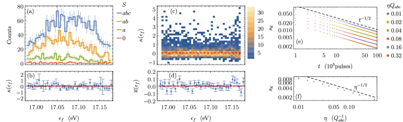
To account for experimental data acquisition, we perform a Monte Carlo simulation: First, we set the experiment’s efficiency such that for the path-configuration about electrons per laser pulse are expected in the considered energy window [51]. To this end, we define , with , where is the transition probability calculated via the transition amplitudes (3) in the absence of noise for the final energy , and . Background-signal counts are considered to appear independently of the final energy with an expected rate of per laser pulse in the considered energy window. For each path-configuration , we then generate a random set of laser parameters , calculate the corresponding detection probabilities for all final energies , and generate a single random sample from the distribution , with the last element corresponding to no click in the considered energy window. By repeating this procedure times (i.e., for laser pulses, taking approximately with a laser [51]), we obtain a histogram for each path-configuration that simulates the detector click statistics in the considered energy window [Fig. 2(a)]. From these, we extract the Sorkin parameter [see Eq. (1)] as a function of the final energy and calculate its precision under consideration of a Poisson error for the detector click statistics [Fig. 2(b)]. Repeating this procedure (i.e., the extraction of the spectrally resolved Sorkin parameter) times results in a distribution of the Sorkin parameter as a function of the final energy [Fig. 2(c)]. Note that for a typical laser repetition frequency of [51], the acquisition of spectrally resolved values of (each resulting from the accumulation of laser pulses) takes about , which is compatible with typical experimentally achievable temporal stabilities [51].
Figure 2(b) shows that the expected precision of a single spectrally resolved Sorkin parameter is typically of the order . When taking the weighted arithmetic mean 111Note that, due to correlations between the numerator and denominator in the definition of the Sorkin parameter from Eq. (1), a bias towards a non-vanishing number can occur when averaging over multiple values of the Sorkin parameter [37]. In order to avoid this bias, we calculate the weighted arithmetic mean by taking the weighted arithmetic means of the numerator and of the denominator in (1) separately., over all generated values of , the standard error , i.e., the precision of the Sorkin parameter, improves by an order of magnitude [Fig. 2(d)], since scales with the inverse square root of the number of values of . By additionally taking the weighted arithmetic mean over the final energies [63], we ultimately obtain the Sorkin parameter with an expected precision of the order .
Finally, we assess the precision of the expected Sorkin parameter as a function of the measurement time and of the experimental data acquisition efficiency . As evident from the linear behavior on the double-logarithmic scale of Figs. 2(e,f), the standard error follows a power law both with respect to the measurement time (provided in units of measured laser pulses), , and data acquisition efficiency, . In the former case, the exponent is due to the scaling of the standard error under repeated measurements, and in the latter case due to the Poisson error of the detector click statistics, which scales with the inverse square root of the number of detected events.
Discussion – The proposed implementation of three-path interference in the energy domain benefits from the intrinsic stability of the paths’ relative phases, where phase noise is due to noise in the well-controllable XUV and IR laser pulses. At the same time, by adjusting the IR spectral components and their time delays , it is possible to change the relative phases between the paths, and, hence, to systematically examine the Sorkin parameter as a function of these relative phases.
The inherent phase stability makes the proposed photoionization-based three-path interferometer also a promising candidate for the Peres test [47], which has only rarely been implemented [46, 44] due to its sensitivity to instabilities in the relative phases between the paths [64]. It examines the exclusion of quaternionic quantum mechanics [65] (a reformulation of quantum mechanics via quaternionic instead of complex numbers) through the measurement of the so-called Peres parameter , with indicating the admissibility of quaternionic quantum mechanics, while complex quantum mechanics is admissible if , and implies the violation of the superposition principle [47]. Similar to the Sorkin parameter , the Peres parameter is a function of the probabilities corresponding to different path-configurations 222In particular, , where , , and [47]., and can thus be computed from the same data set from which we obtained Figs. 2(c,d), resulting in the mean Peres parameter 333For each path-configuration, we sum all counts sampled from laser pulses with data acquisition efficiency , and subtract the simulated dark counts. We then calculate the spectrally resolved Peres parameter (see [66]), and finally calculate the weighted arithmetic mean over all final energies .. Since all our simulations were performed according to the rules of standard (complex) quantum mechanics, the slight deviation from unity suggests that reduced experimental noise (as compared to the noise levels here assumed) will be required to establish the Peres test as an experimental benchmark with discriminative power.
Acknowledgements.
The authors are grateful to Anne L’Huillier for fruitful discussions. D.B and C.D. acknowledge financial support from the Knut and Alice Wallenberg Foundation through the Wallenberg Centre for Quantum Technology (WACQT). C.D. acknowledges financial support from the European Research Council (Advanced grant QPAP), and support by the Georg H. Endress foundation. D.B. acknowledges support from the Swedish Research Council grant 2020-06384.References
- Krausz and Ivanov [2009] F. Krausz and M. Ivanov, Attosecond physics, Reviews of Modern Physics 81, 163 (2009).
- Calegari et al. [2016] F. Calegari, G. Sansone, S. Stagira, C. Vozzi, and M. Nisoli, Advances in attosecond science, Journal of Physics B: Atomic, Molecular and Optical Physics 49, 062001 (2016).
- Kienberger et al. [2004] R. Kienberger, E. Goulielmakis, M. Uiberacker, A. Baltuska, V. Yakovlev, F. Bammer, A. Scrinzi, T. Westerwalbesloh, U. Kleineberg, U. Heinzmann, M. Drescher, and F. Krausz, Atomic transient recorder, Nature 427, 817 (2004).
- Sansone et al. [2006] G. Sansone, E. Benedetti, F. Calegari, C. Vozzi, L. Avaldi, R. Flammini, L. Poletto, P. Villoresi, C. Altucci, R. Velotta, S. Stagira, S. D. Silvestri, and M. Nisoli, Isolated single-cycle attosecond pulses, Science 314, 443 (2006).
- Bergues et al. [2012] B. Bergues, M. Kübel, N. G. Johnson, B. Fischer, N. Camus, K. J. Betsch, O. Herrwerth, A. Senftleben, A. M. Sayler, T. Rathje, T. Pfeifer, I. Ben-Itzhak, R. R. Jones, G. G. Paulus, F. Krausz, R. Moshammer, J. Ullrich, and M. F. Kling, Attosecond tracing of correlated electron-emission in non-sequential double ionization, Nature Communications 3, 813 (2012).
- Kaldun et al. [2016] A. Kaldun, A. Blättermann, V. Stooß, S. Donsa, H. Wei, R. Pazourek, S. Nagele, C. Ott, C. D. Lin, J. Burgdörfer, and T. Pfeifer, Observing the ultrafast buildup of a Fano resonance in the time domain, Science 354, 738 (2016).
- Sansone et al. [2010] G. Sansone, F. Kelkensberg, J. F. Pérez-Torres, F. Morales, M. F. Kling, W. Siu, O. Ghafur, P. Johnsson, M. Swoboda, E. Benedetti, F. Ferrari, F. Lépine, J. L. Sanz-Vicario, S. Zherebtsov, I. Znakovskaya, A. L’Huillier, M. Y. Ivanov, M. Nisoli, F. Martín, and M. J. J. Vrakking, Electron localization following attosecond molecular photoionization, Nature 465, 763 (2010).
- Gong et al. [2023] X. Gong, É. Plésiat, A. Palacios, S. Heck, F. Martín, and H. J. Wörner, Attosecond delays between dissociative and non-dissociative ionization of polyatomic molecules, Nature Communications 14, 4402 (2023).
- Cavalieri et al. [2007] A. L. Cavalieri, N. Müller, T. Uphues, V. S. Yakovlev, A. Baltuška, B. Horvath, B. Schmidt, L. Blümel, R. Holzwarth, S. Hendel, M. Drescher, U. Kleineberg, P. M. Echenique, R. Kienberger, F. Krausz, and U. Heinzmann, Attosecond spectroscopy in condensed matter, Nature 449, 1029 (2007).
- Paul et al. [2001] P. M. Paul, E. S. Toma, P. Breger, G. Mullot, F. Augé, P. Balcou, H. G. Muller, and P. Agostini, Observation of a train of attosecond pulses from high harmonic generation, Science 292, 1689 (2001).
- Kotur et al. [2016] M. Kotur, D. Guénot, Á. Jiménez-Galán, D. Kroon, E. W. Larsen, M. Louisy, S. Bengtsson, M. Miranda, J. Mauritsson, C. L. Arnold, S. E. Canton, M. Gisselbrecht, T. Carette, J. M. Dahlström, E. Lindroth, A. Maquet, L. Argenti, F. Martín, and A. L’Huillier, Spectral phase measurement of a Fano resonance using tunable attosecond pulses, Nature Communications 7, 10566 (2016).
- Gruson et al. [2016] V. Gruson, L. Barreau, A. Jiménez-Galan, F. Risoud, J. Caillat, A. Maquet, B. Carré, F. Lepetit, J.-F. Hergott, T. Ruchon, L. Argenti, R. Taïeb, F. Martín, and P. Saliéres, Attosecond dynamics through a Fano resonance: Monitoring the birth of a photoelectron, Science 354, 734 (2016).
- Busto et al. [2018] D. Busto, L. Barreau, M. Isinger, M. Turconi, C. Alexandridi, A. Harth, S. Zhong, R. J. Squibb, D. Kroon, S. Plogmaker, M. Miranda, A. Jiménez-Galán, L. Argenti, C. L. Arnold, R. Feifel, F. Martín, M. Gisselbrecht, A. L’Huillier, and P. Salières, Time–frequency representation of autoionization dynamics in helium, Journal of Physics B: Atomic, Molecular and Optical Physics 51, 044002 (2018).
- Priebe et al. [2017] K. E. Priebe, C. Rathje, S. V. Yalunin, T. Hohage, A. Feist, S. Schäfer, and C. Ropers, Attosecond electron pulse trains and quantum state reconstruction in ultrafast transmission electron microscopy, Nature Photonics 11, 793 (2017).
- Bourassin-Bouchet et al. [2020] C. Bourassin-Bouchet, L. Barreau, V. Gruson, J.-F. Hergott, F. Quéré, P. Salières, and T. Ruchon, Quantifying decoherence in attosecond metrology, Physical Review X 10, 031048 (2020).
- Laurell et al. [2022] H. Laurell, D. Finkelstein-Shapiro, C. Dittel, C. Guo, R. Demjaha, M. Ammitzböll, R. Weissenbilder, L. Neoričić, S. Luo, M. Gisselbrecht, C. L. Arnold, A. Buchleitner, T. Pullerits, A. L’Huillier, and D. Busto, Continuous-variable quantum state tomography of photoelectrons, Physical Review Research 4, 033220 (2022).
- Laurell et al. [2023] H. Laurell, S. Luo, R. Weissenbilder, M. Ammitzböll, S. Ahmed, H. Söderberg, C. L. M. Petersson, V. Poulain, C. Guo, C. Dittel, D. Finkelstein-Shapiro, R. J. Squibb, R. Feifel, M. Gisselbrecht, C. L. Arnold, A. Buchleitner, E. Lindroth, A. F. Kockum, A. L’Huillier, and D. Busto, Measuring the quantum state of photoelectrons, arXiv:2309.13945 (2023).
- Tichy et al. [2011] M. C. Tichy, F. Mintert, and A. Buchleitner, Essential entanglement for atomic and molecular physics, Journal of Physics B: Atomic, Molecular and Optical Physics 44, 192001 (2011).
- Lewenstein et al. [2022] M. Lewenstein, N. Baldelli, U. Bhattacharya, J. Biegert, M. Ciappina, U. Elu, T. Grass, P. Grochowski, A. Johnson, T. Lamprou, A. Maxwell, A. O. nez, E. Pisanty, J. Rivera-Dean, P. Stammer, I. Tyulnev, and P. Tzallas, Attosecond physics and quantum information science, arXiv:2208.14769 (2022).
- Akoury et al. [2007] D. Akoury, K. Kreidi, T. Jahnke, T. Weber, A. Staudte, M. Schöffler, N. Neumann, J. Titze, L. P. H. Schmidt, A. Czasch, O. Jagutzki, R. A. C. Fraga, R. E. Grisenti, R. D. Muiño, N. A. Cherepkov, S. K. Semenov, P. Ranitovic, C. L. Cocke, T. Osipov, H. Adaniya, J. C. Thompson, M. H. Prior, A. Belkacem, A. L. Landers, H. Schmidt-Böcking, and R. Dörner, The simplest double slit: Interference and entanglement in double photoionization of H2, Science 318, 949 (2007).
- Zimmermann et al. [2008] B. Zimmermann, D. Rolles, B. Langer, R. Hentges, M. Braune, S. Cvejanovic, O. Geßner, F. Heiser, S. Korica, T. Lischke, A. Reinköster, J. Viefhaus, R. Dörner, V. McKoy, and U. Becker, Localization and loss of coherence in molecular double-slit experiments, Nature Physics 4, 649 (2008).
- Langer and Becker [2009] B. Langer and U. Becker, Localization and loss of coherence in molecular double slit experiments, Journal of Physics: Conference Series 194, 022003 (2009).
- Vrakking [2021] M. J. J. Vrakking, Control of attosecond entanglement and coherence, Physical Review Letters 126, 113203 (2021).
- Koll et al. [2022] L.-M. Koll, L. Maikowski, L. Drescher, T. Witting, and M. J. J. Vrakking, Experimental control of quantum-mechanical entanglement in an attosecond pump-probe experiment, Physical Review Letters 128, 043201 (2022).
- Stammer et al. [2023] P. Stammer, J. Rivera-Dean, A. Maxwell, T. Lamprou, A. Ordóñez, M. F. Ciappina, P. Tzallas, and M. Lewenstein, Quantum electrodynamics of intense laser-matter interactions: A tool for quantum state engineering, PRX Quantum 4, 010201 (2023).
- Gorlach et al. [2023] A. Gorlach, M. E. Tzur, M. Birk, M. Krüger, N. Rivera, O. Cohen, and I. Kaminer, High-harmonic generation driven by quantum light, Nature Physics 19, 1689 (2023).
- Bhattacharya et al. [2023] U. Bhattacharya, T. Lamprou, A. S. Maxwell, A. Ordóñez, E. Pisanty, J. Rivera-Dean, P. Stammer, M. F. Ciappina, M. Lewenstein, and P. Tzallas, Strong–laser–field physics, non–classical light states and quantum information science, Reports on Progress in Physics 86, 094401 (2023).
- Cohen-Tannoudji et al. [2019] C. Cohen-Tannoudji, B. Diu, and F. Laloë, Quantum Mechanics, Volume 1: Basic Concepts, Tools, and Applications (Wiley, 2019).
- Born [1926] M. Born, Zur Quantenmechanik der Stoßvorgänge, Zeitschrift für Physik 37, 863 (1926).
- Sorkin [1994] R. D. Sorkin, Quantum mechanics as quantum measure theory, Modern Physics Letters A 09, 3119 (1994).
- Dakić et al. [2014] B. Dakić, T. Paterek, and Č Brukner, Density cubes and higher-order interference theories, New Journal of Physics 16, 023028 (2014).
- Życzkowski [2008] K. Życzkowski, Quartic quantum theory: an extension of the standard quantum mechanics, Journal of Physics A 41, 355302 (2008).
- Sinha et al. [2010] U. Sinha, C. Couteau, T. Jennewein, R. Laflamme, and G. Weihs, Ruling out multi-order interference in quantum mechanics, Science 329, 418 (2010).
- Söllner et al. [2011] I. Söllner, B. Gschösser, P. Mai, B. Pressl, Z. Vörös, and G. Weihs, Testing Born’s rule in quantum mechanics for three mutually exclusive events, Foundations of Physics 42, 742 (2011).
- Hickmann et al. [2011] J. M. Hickmann, E. J. S. Fonseca, and A. J. Jesus-Silva, Born’s rule and the interference of photons with orbital angular momentum by a triangular slit, Europhysics Letters 96, 64006 (2011).
- Magaña-Loaiza et al. [2016] O. S. Magaña-Loaiza, I. De Leon, M. Mirhosseini, R. Fickler, A. Safari, U. Mick, B. McIntyre, P. Banzer, B. Rodenburg, G. Leuchs, and R. W. Boyd, Exotic looped trajectories of photons in three-slit interference, Nature Communications 7, 13987 (2016).
- Kauten et al. [2017] T. Kauten, R. Keil, T. Kaufmann, B. Pressl, Č . Brukner, and G. Weihs, Obtaining tight bounds on higher-order interferences with a 5-path interferometer, New Journal of Physics 19, 033017 (2017).
- Vogl et al. [2021] T. Vogl, H. Knopf, M. Weissflog, P. K. Lam, and F. Eilenberger, Sensitive single-photon test of extended quantum theory with two-dimensional hexagonal boron nitride, Physical Review Research 3, 013296 (2021).
- Park et al. [2012] D. K. Park, O. Moussa, and R. Laflamme, Three path interference using nuclear magnetic resonance: a test of the consistency of Born’s rule, New Journal of Physics 14, 113025 (2012).
- Jin et al. [2017] F. Jin, Y. Liu, J. Geng, P. Huang, W. Ma, M. Shi, C.-K. Duan, F. Shi, X. Rong, and J. Du, Experimental test of Born’s rule by inspecting third-order quantum interference on a single spin in solids, Physical Review A 95, 012107 (2017).
- Barnea et al. [2018] A. R. Barnea, O. Cheshnovsky, and U. Even, Matter-wave diffraction approaching limits predicted by Feynman path integrals for multipath interference, Physical Review A 97, 023601 (2018).
- Cotter et al. [2017] J. P. Cotter, C. Brand, C. Knobloch, Y. Lilach, O. Cheshnovsky, and M. Arndt, In search of multipath interference using large molecules, Science Advances 3, e1602478 (2017).
- Pleinert et al. [2021] M.-O. Pleinert, A. Rueda, E. Lutz, and J. von Zanthier, Testing higher-order quantum interference with many-particle states, Physical Review Letters 126, 190401 (2021).
- Conlon et al. [2024] L. O. Conlon, A. Walsh, Y. Hua, OThearle, T. Vogl, F. Eilenberger, P. K. Lam, and S. M. Assad, Testing the postulates of quantum mechanics with coherent states of light and homodyne detection, New Journal of Physics 26, 053003 (2024).
- Gstir [2023] S. Gstir, Waveguide Interferometers for Fundamental Investigation of Quantum Mechanics, Ph.D. thesis, University of Innsbruck (2023), urn:nbn:at:at-ubi:1-128187.
- Sadana et al. [2022] S. Sadana, L. Maccone, and U. Sinha, Testing quantum foundations with quantum computers, Physical Review Research 4, L022001 (2022).
- Peres [1979] A. Peres, Proposed test for complex versus quaternion quantum theory, Physical Review Letters 42, 683 (1979).
- Lee et al. [2020] K. S. Lee, Z. Zhuo, C. Couteau, D. Wilkowski, and T. Paterek, Atomic test of higher-order interference, Physical Review A 101, 052111 (2020).
- Villeneuve et al. [2017] D. M. Villeneuve, P. Hockett, M. J. J. Vrakking, and H. Niikura, Coherent imaging of an attosecond electron wave packet, Science 356, 1150 (2017).
- Barreau et al. [2019] L. Barreau, C. L. M. Petersson, M. Klinker, A. Camper, C. Marante, T. Gorman, D. Kiesewetter, L. Argenti, P. Agostini, J. González-Vázquez, P. Salières, L. F. DiMauro, and F. Martín, Disentangling spectral phases of interfering autoionizing states from attosecond interferometric measurements, Physical Review Letters 122, 253203 (2019).
- Luo et al. [2023] S. Luo, R. Weissenbilder, H. Laurell, M. Ammitzböll, V. Poulain, D. Busto, L. Neoričić, C. Guo, S. Zhong, D. Kroon, R. J. Squibb, R. Feifel, M. Gisselbrecht, A. L’Huillier, and C. L. Arnold, Ultra-stable and versatile high-energy resolution setup for attosecond photoelectron spectroscopy, Advances in Physics: X 8, 2250105 (2023).
- Agostini et al. [1979] P. Agostini, F. Fabre, G. Mainfray, G. Petite, and N. K. Rahman, Free-free transitions following six-photon ionization of xenon atoms, Physical Review Letters 42, 1127 (1979).
- Jiménez-Galán et al. [2016] A. Jiménez-Galán, F. Martín, and L. Argenti, Two-photon finite-pulse model for resonant transitions in attosecond experiments, Physical Review A 93, 023429 (2016).
- Förderer [2022] P. Förderer, Testing Born’s rule via photoionization of helium, B.Sc. thesis, Albert-Ludwigs-Universität Freiburg, urn:nbn:de:bsz:25-freidok-2513227 10.6094/UNIFR/251322 (2022).
- Cohen-Tannoudji et al. [1998] C. Cohen-Tannoudji, J. Dupont-Roc, and G. Grynberg, Atom – Photon Interactions: Basic Process and Applications (John Wiley & Sons, Ltd, 1998).
- Sawant et al. [2014] R. Sawant, J. Samuel, A. Sinha, S. Sinha, and U. Sinha, Nonclassical paths in quantum interference experiments, Physical Review Letters 113, 120406 (2014).
- Sinha et al. [2015] A. Sinha, A. H. Vijay, and U. Sinha, On the superposition principle in interference experiments, Scientific Reports 5, 10304 (2015).
- Namdar et al. [2023] P. Namdar, P. K. Jenke, I. A. Calafell, A. Trenti, M. Radonjić, B. Dakić, P. Walther, and L. A. Rozema, Experimental higher-order interference in a nonlinear triple slit, Physical Review A 107, 032211 (2023).
- Fano [1961] U. Fano, Effects of configuration interaction on intensities and phase shifts, Physical Review 124, 1866 (1961).
- Domke et al. [1996] M. Domke, K. Schulz, G. Remmers, G. Kaindl, and D. Wintgen, High-resolution study of 1 double-excitation states in helium, Physical Review A 53, 1424 (1996).
- Fano [1985] U. Fano, Propensity rules: An analytical approach, Physical Review A 32, 617 (1985).
- Busto et al. [2019] D. Busto, J. Vinbladh, S. Zhong, M. Isinger, S. Nandi, S. Maclot, P. Johnsson, M. Gisselbrecht, A. L’Huillier, E. Lindroth, and J. M. Dahlström, Fano’s propensity rule in angle-resolved attosecond pump-probe photoionization, Physical Review Letters 123, 133201 (2019).
- Note [1] Note that, due to correlations between the numerator and denominator in the definition of the Sorkin parameter from Eq. (1\@@italiccorr), a bias towards a non-vanishing number can occur when averaging over multiple values of the Sorkin parameter [37]. In order to avoid this bias, we calculate the weighted arithmetic mean by taking the weighted arithmetic means of the numerator and of the denominator in (1\@@italiccorr) separately.
- Gstir et al. [2021] S. Gstir, E. Chan, T. Eichelkraut, A. Szameit, R. Keil, and G. Weihs, Towards probing for hypercomplex quantum mechanics in a waveguide interferometer, New Journal of Physics 23, 093038 (2021).
- Adler [1995] S. L. Adler, Quaternionic Quantum Mechanics and Quantum Fields, International series of monographs on physics (Oxford University Press, 1995).
- Note [2] In particular, , where , , and [47].
- Note [3] For each path-configuration, we sum all counts sampled from laser pulses with data acquisition efficiency , and subtract the simulated dark counts. We then calculate the spectrally resolved Peres parameter (see [66]), and finally calculate the weighted arithmetic mean over all final energies .