Chiral Dissociation of Bound Photon Pairs for a Non-Hermitian Skin Effect
Abstract
We theoretically study the bound states of interacting photons propagating in a waveguide chirally coupled to an array of atoms. We demonstrate that the bound photon pairs can concentrate at the edge of the array and link this to the non-Hermitian skin effect. Unlike tight-binding non-Hermitian setups, the bound states in the waveguide-coupled array exhibit infinite radiative lifetimes when the array has an infinite size. However, in a finite array, non-Hermiticity and localization of bound pairs emerge due to their chiral dissociation into scattering states. Counterintuitively, when the photons are preferentially emitted to the right, the bound pairs are localized at the left edge of the array and vice versa.
Introduction. Non-Hermitian skin effect (NHSE) has now become the paradigmatic example of the topologically nontrivial effects of loss or gain in optical and condensed matter systems [1, 2, 3, 4, 5, 6, 7, 8]. Namely, if the energy spectrum as a function of the momentum forms a loop in a complex plane, the macroscopic fraction of the eigenmodes in the finite-size structure with open boundary conditions is localized at the edge. Typically, such complex-valued loops of the energy spectrum arise due to local loss or gain, or unequal forward and backward tunneling links [9]. The loss can also be nonlocal; for example, it can result from the collective spontaneous emission of photons into the far field [10]. Recently, NHSE has also been investigated in the quantum setup in the presence of interactions [11, 12, 13, 14, 15]. In particular, it has been shown that two interacting particles with different masses can get localized at an edge, even if the structure is Hermitian and time-reversal symmetry is preserved [13]. These results suggest the presence of other unchartered mechanisms for NHSE in interacting systems.
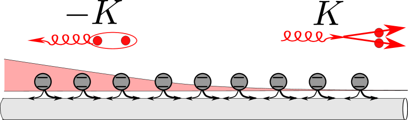
In this Letter, we consider the non-Hermitian skin effect for a composite particle. We focus on two photons bound via atom-mediated interactions, as illustrated in Fig. 1. Such bound pairs can be realized for cold atom systems [16, 17, 18] and have also been predicted for microwave photons coupled to superconducting qubits setup [19]. Contrary to the previously studied mechanisms, here, the non-Hermiticity, essential for NHSE, is provided neither by loss nor gain but just by an intrinsic feature of the bound pair: its dissociation into scattering states.
Before proceeding to the rigorous theoretical model, we present a qualitative explanation of the proposed mechanism. We start with the dispersion relation for the bound pair, , schematically illustrated in Fig. 2(a), here is the center-of-mass momentum. The thick black and thin blue curves correspond to chiral and non-chiral structures, respectively. The black curve lacks mirror symmetry; . Chirality is an essential ingredient for this NHSE mechanism. The second essential ingredient is the presence of a continuum of scattering states, represented by the shaded area in Fig. 2(a). This means that the bound states dissociate and cease to exist when their momentum is in a certain range. Our main observation is that due to the chirality of the system, there exists a range of the energies belonging to the bound state spectrum in Fig. 2(a), indicated by the black circles, where takes only negative values and group velocity has only a negative sign. The “unidirectional” range is a consequence of the scattering continuum that renders the dispersion law non-analytical. Without such a continuum, there has to be an even number of the solutions for the equation because of the bound state branch continuity and periodicity, . One can then expect that the bound eigenstates in the finite structure will become standing waves of the type
| (1) |
where is the pair of solutions and is the center of mass coordinate. The scattering continuum can destroy one of these two solutions, making the bound state unidirectional. We will demonstrate that the bound states, corresponding to the unidirectional spectral range, will be localized at the edge under open boundary conditions, which can be interpreted as an analog of NHSE, as illustrated in Fig. 1. This loss mechanism is rather special: in an infinite structure, the portions of the dispersion curve corresponding to bound states outside the scattering continuum are real-valued, meaning the bound pairs have an infinite lifetime for a fixed value of . This is a qualitative difference from non-reciprocal tight-binding Bose-Hubbard-type models [11, 12, 14, 15], where is complex-valued. However, in a finite array, considered bound states acquire a finite lifetime and become localized at the structure’s edge.
Waveguide quantum electrodynamics model. We now discuss the specific implementation of the proposed dissociation-driven NHSE in an array of two-level atoms chirally coupled to a waveguide, see Fig. 1. The single-particle eigenstates are polaritons, formed by the hybridization of photons with a linear dispersion relation and atoms with resonance frequency . Due to chirality, the Rabi splittings at the two avoided crossings of the polariton dispersion curve for positive and negative have different values (see Fig. S1 in 111Online Supplementary Materials).
We focus on the bound double-excited states where the wavefunction has the form and the two-photon amplitude decays with the distance between the two excitations . Here, are the raising operators for the atoms. The structure of double-excited states in this model, known for a long time [21, 22, 23], has received significant attention in the last several years [19, 24, 25, 26, 27, 28, 29, 30], including the study of the chiral systems [31, 30, 32, 33], see in particular Refs. [30, 32] for the chiral bound states, that were also observed in experiment [18]. However, the general connection of the chiral bound pair dissociation to the non-Hermitian skin effect manifested as a spectral range of edge-localized bound states, to the best of our knowledge, has remained completely unexplored.
The effective non-Hermitian Hamiltonian of the structure is given by [34, 10]
| (2) |
Here, is the atom resonant frequency, and , are the spontaneous decay rates into the waveguide in the forward and backward directions, respectively. The parameter represents the phase gained by light propagating the distance between adjacent atoms with the velocity . The Hamiltonian Eq. (2) is written in the Markovian approximation with traced-out photon modes, which is valid for . The chirality of the structure is quantified by the parameter , that is the ratio of emission rates in the forward and backward directions. The non-chiral case corresponds to . The array features long-ranged waveguide-mediated coupling.
When the structure has translational symmetry, the center-of-mass wave vector is a good quantum number and the two-photon wave function can be sought in the form
| (3) |
The bound pair dispersion law can be found by diagonalizing the following Hamiltonian [32]:
| (4) | ||||
and .
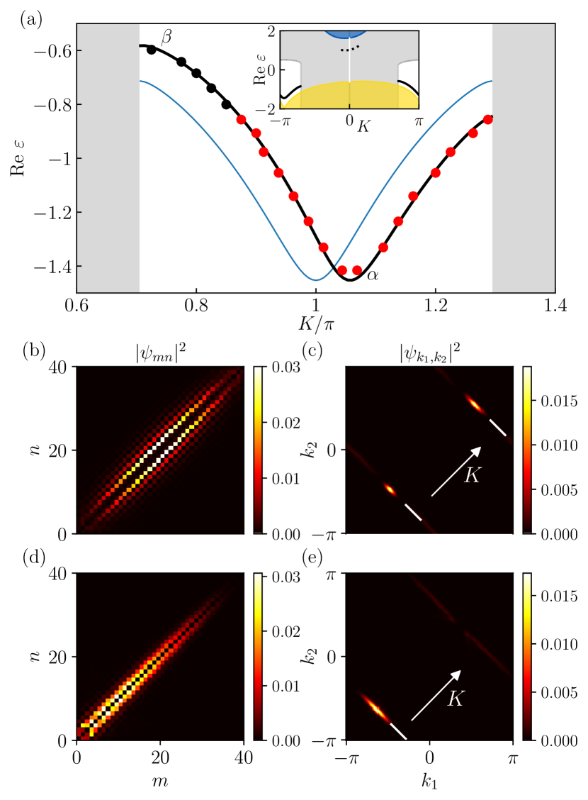
The results of the calculations are shown by the curves in Fig. 2(a). We focus on a single branch of the bound states that, in the limit of vanishing chirality, has the energy [27] at . This branch is formed by binding the polaritons with the two dispersion branches, the upper one with and the bottom one with . Due to the avoided crossing at , where the single-polariton dispersion diverges in the Markovian approximation [34, 20], the bound states exist only for . For , they dissociate into the continuum (gray areas in the left and right parts of Fig. 2a) and become resonance states [30]. The inset of Fig. 2(a) also presents the two-photon dispersion in a broad energy and wave vector range.
Near the edge of the Brillouin zone, the pair dispersion law can be approximated by a Taylor series:
| (5) |
Here, is the effective mass of the bound pair. It has been calculated analytically for in Ref. [27]. The linear-in- term appears only for the nonvanishing chirality. In the lowest order in this term can be calculated by the usual perturbation theory [20]:
| (6) |
As a result of the chirality, the extremum of the dispersion curve shifts from the point and the curve loses mirror symmetry around the point ; ; compare black and blue curves in Fig. 2(a). As discussed in the introduction, the breakdown of mirror symmetry and the absence of the bound states for means that there is a unidirectional part of the dispersion curve when the equation has only one solution. We stress that the pair dispersion in the infinite periodic structure stays real outside the gray area. This distinguishes considered waveguide setup from systems with local losses or gain at each site, such as the Hatano-Nelson model [9], that have complex spectrum under the periodic boundary conditions.
We now calculate the eigenstates in the finite-size array with atoms. This is done by direct numerical diagonalization of the Hamiltonian Eq. (2), without assuming translational symmetry. For each two-photon amplitude we also calculate the corresponding Fourier transform . Panels (b-e) in Fig. 2 present the two-photon amplitudes (b,d) and their Fourier transforms (c,e) for two characteristic bound states and , indicated in the dispersion branch in Fig. 2(a). For each state, we numerically extract the corresponding center of mass wave vectors from the positions of the maxima of the Fourier transform . The corresponding momenta are indicated in Fig. 2(c,e) by thin white lines perpendicular to the axis, shown by white arrows. Next, we put a circle at the energy equal to and the extracted momentum on the dispersion plot Fig. 2(a). The results demonstrate a good agreement between the dispersion of the pairs in the infinite structure with the periodic boundary conditions and the dispersion of the same pairs in a finite structure. This agreement can be interpreted as the pair being quantized in the finite array as a single composite particle, given that the array size significantly exceeds the pair size. This behavior is analogous to exciton quantization as a whole in wide semiconductor quantum wells [35].
For most of the bound states, there exist two maxima and in the Fourier transform (red circles in Fig. 2a). This is quite natural: the bound pair forms a standing wave in the finite-size array, and a standing wave has two Fourier components. We term such states “bidirectional”. Our main finding is the presence of “unidirectional” bound states with just one distinct maxima for . These are indicated by black circles in Fig. 2(a) and correspond to the unidirectional part of the bulk dispersion branch. We show in Fig. 2(d) that these “unidirectional” states are concentrated at the edge of the structure, in stark contrast to the bidirectional states. In the non-chiral case the unidirectional states are absent, see supplementary Fig. S3 in [20]. Counterintuitively, the bound states in the chiral structure are concentrated at the left edge, even though the calculation has been performed for . Opposite edge localization can be explained by the negative sign of the polariton group velocity. It may still seem contradictory since for (), all the states should be localized on the right edge [10]. We show in [20] that the binding energy tends to zero in this limit, and the considered bound state disappears by merging with the continuum. This resolves the apparent contradiction.
Non-Hermitian skin effect for bound states. The concentration of the bound pairs on the structure edge is a strong indication of the non-Hermitian skin effect. The specific mechanism of non-Hermiticity and losses requires a more analytical investigation. To this end, we now present an effective model for the composite bound states that allows us to distill the mechanisms for the results in Fig. 2. We consider an effective pair Hamiltonian given by
| (7) |
where is an annihilation operator for a single bound pair. The first term in Eq. (7) describes the chiral dispersion of a bound pair moving on a one-dimensional lattice. The parameter is the real tunneling amplitude, and the phase characterizes the chirality of the tunneling. This phase introduces an asymmetry in the hopping between neighboring lattice sites, breaking the time-reversal symmetry.
The second term in Eq. (7) is more complicated. We have introduced it to phenomenologically describe the loss the bound pair experiences when the center-of-mass momentum of a pair is in a certain range . This -dependent loss can be formally implemented by a Fourier transform
| (8) |
where describes the momentum-dependent loss. We assign to be equal to for and 0 otherwise. In our actual numerical calculation, instead of the step-functions, we use the sigmoidal-type functions, that is
| (9) |
Here, the parameter is the finite step width for the loss function in the momentum space.
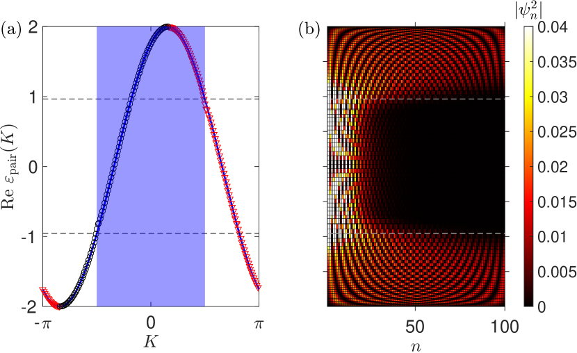
The results of calculating the eigenstates of the effective pair Hamiltonian Eq. (7) are shown in Fig. 3. Panel (a) presents the real parts of the energies of the eigenstates. The thin curve shows the pair spectrum in the infinite structure with the periodic boundary conditions, described by the following equation
| (10) |
The dispersion curve manifests the chirality of the structure: it has the reflection symmetry around the point , shifted from the origin.
The triangles and circles present the results of the numerical calculation for a finite structure. Inspired by the results in Fig. 2 we expect that each eigenstate of Eq. (7) can be approximated by a sum of two plane waves, see Eq. (1). In order to extract the real parts of the wave vectors we calculate the Fourier transform of the wavefunction amplitude and assign to the two maxima of . Next, we show the real parts of the eigenenergies versus () by black triangles (red cicles). The results perfectly agree with the spectrum in the infinite structure Eq. (10) (blue curve).
Similarly to Fig. 2, we use blue shading in Fig. 3(a) to indicate the region of large loss. The spectral region between the two horizontal lines is the unidirectional range of energies , where the imaginary parts for the two solutions differ significantly, and we expect the modes to accumulate at the structure edge. As expected, the unidirectional energy range indeed corresponds to the eigenstates concentrated on the edge. We have confirmed that the localization is exponential and can be switched from the left edge to the right one by changing the sign of the chirality parameter (Fig. S4 in [20]).
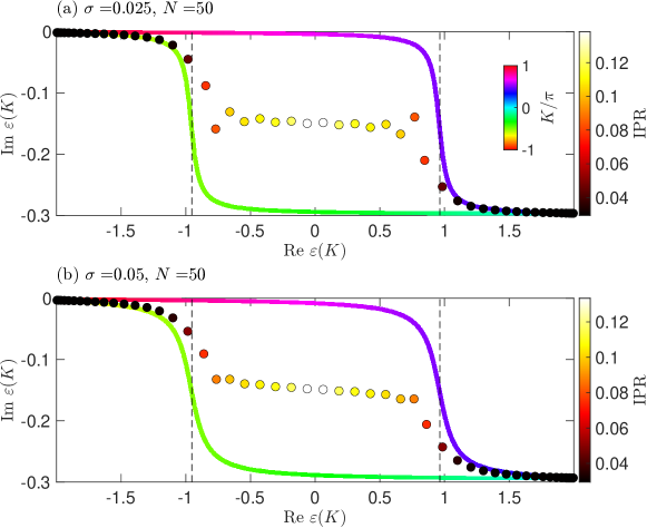
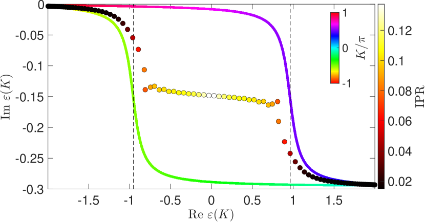
Finally, Fig. 4 shows the energy dispersion Eq. (10) in the complex plane. The dispersion curve has a characteristic loop with a nonzero winding number as a function of . The extent of the loop is regulated by the complex -dependent term . Meanwhile, the energy spectrum for the open boundary conditions, shown in Fig. 4 by colored circles, forms a single curve. The circle color represents the localization degree of the eigenstates, quantified by the inverse participation ratio (IPR), defined as . More localized eigenstates (brighter circles) correspond to the center of the loop in the periodic structure. Such a loop collapse into a curve is a hallmark of the NHSE. We have also checked that the results do not qualitatively depend on and once the effective broadening of the momenta in the finite system [20]. Thus, our effective single-composite-particle model links the localization observed for the two-particle bound states in Fig. 2 to the NHSE.
Summary. To summarize, we have demonstrated that the dissociation of bound pairs in a chiral structure can result in the non-Hermitian skin effect, where the pairs are localized at the edge. We illustrated the mechanism for a specific platform of waveguide quantum electrodynamics, where photons propagating in one dimension are coupled to atoms in a waveguide. The coexistence of the continuum with the quasiparticle dispersion branch is a generic feature for the energy spectra of various many-body systems, for example, with plasmonic or magnonic excitations [36]. Once the time-reversal symmetry is broken, the quasiparticle branch acquires a unidirectional part. Therefore, we believe that our results could apply beyond one-dimensional systems and beyond setups with atom-photon coupling.
We thank Ekaterina Vlasiuk and Janet Zhong for valuable discussions. The work of A.N.P. has been supported by research grants from the Minerva Foundation, from the Center for New Scientists, and the Center for Scientific Excellence at the Weizmann Institute of Science.
References
- Lee [2016] T. E. Lee, Anomalous edge state in a non-Hermitian lattice, Phys. Rev. Lett. 116, 133903 (2016).
- Martinez Alvarez et al. [2018] V. M. Martinez Alvarez, J. E. Barrios Vargas, and L. E. F. Foa Torres, Non-Hermitian robust edge states in one dimension: Anomalous localization and eigenspace condensation at exceptional points, Phys. Rev. B 97, 121401 (2018).
- Kunst et al. [2018] F. K. Kunst, E. Edvardsson, J. C. Budich, and E. J. Bergholtz, Biorthogonal bulk-boundary correspondence in non-Hermitian systems, Phys. Rev. Lett. 121, 026808 (2018).
- Yao and Wang [2018] S. Yao and Z. Wang, Edge states and topological invariants of non-Hermitian systems, Phys. Rev. Lett. 121, 086803 (2018).
- Zhang et al. [2020a] K. Zhang, Z. Yang, and C. Fang, Correspondence between winding numbers and skin modes in non-Hermitian systems, Phys. Rev. Lett. 125, 126402 (2020a).
- Borgnia et al. [2020] D. S. Borgnia, A. J. Kruchkov, and R.-J. Slager, Non-Hermitian boundary modes and topology, Phys. Rev. Lett. 124, 056802 (2020).
- Okuma et al. [2020] N. Okuma, K. Kawabata, K. Shiozaki, and M. Sato, Topological origin of non-Hermitian skin effects, Phys. Rev. Lett. 124, 086801 (2020).
- Bergholtz et al. [2021] E. J. Bergholtz, J. C. Budich, and F. K. Kunst, Exceptional topology of non-Hermitian systems, Rev. Mod. Phys. 93, 015005 (2021).
- Hatano and Nelson [1997] N. Hatano and D. R. Nelson, Vortex pinning and non-Hermitian quantum mechanics, Phys. Rev. B 56, 8651 (1997).
- Poddubny et al. [2024] A. Poddubny, J. Zhong, and S. Fan, Mesoscopic non-Hermitian skin effect, Phys. Rev. A 109, L061501 (2024).
- Lee [2021] C. H. Lee, Many-body topological and skin states without open boundaries, Phys. Rev. B 104, 195102 (2021).
- Shen and Lee [2022] R. Shen and C. H. Lee, Non-Hermitian skin clusters from strong interactions, Communications Physics 5, 238 (2022).
- Poddubny [2023] A. N. Poddubny, Interaction-induced analog of a non-Hermitian skin effect in a lattice two-body problem, Phys. Rev. B 107, 045131 (2023).
- Brighi and Nunnenkamp [2024] P. Brighi and A. Nunnenkamp, Nonreciprocal dynamics and the non-Hermitian skin effect of repulsively bound pairs, Phys. Rev. A 110, L020201 (2024).
- Wang et al. [2024] H.-Y. Wang, J. Li, W.-M. Liu, L. Wen, and X.-F. Zhang, Exotic localization for the two body bound states in the non-reciprocal Hubbard model (2024), arXiv:2409.07883 [quant-ph] .
- Winkler et al. [2006] K. Winkler, G. Thalhammer, F. Lang, R. Grimm, J. Hecker Denschlag, A. J. Daley, A. Kantian, H. P. Büchler, and P. Zoller, Repulsively bound atom pairs in an optical lattice, Nature (London) 441, 853 (2006).
- Firstenberg et al. [2013] O. Firstenberg, T. Peyronel, Q.-Y. Liang, A. V. Gorshkov, M. D. Lukin, and V. Vuletić, Attractive photons in a quantum nonlinear medium, Nature 502, 71 (2013).
- Prasad et al. [2020] A. S. Prasad, J. Hinney, S. Mahmoodian, K. Hammerer, S. Rind, P. Schneeweiss, A. S. Sørensen, J. Volz, and A. Rauschenbeutel, Correlating photons using the collective nonlinear response of atoms weakly coupled to an optical mode, Nature Photonics 14, 719 (2020).
- Zhang et al. [2020b] Y.-X. Zhang, C. Yu, and K. Mølmer, Subradiant bound dimer excited states of emitter chains coupled to a one dimensional waveguide, Phys. Rev. Research 2, 013173 (2020b).
- Note [1] Online Supplementary Materials.
- Yudson and Rupasov [1984] V. Yudson and V. Rupasov, Exact Dicke superradiance theory: Bethe wavefunctions in the discrete atom model, Sov. Phys. JETP 59, 478 (1984).
- Shen and Fan [2007] J.-T. Shen and S. Fan, Strongly correlated multiparticle transport in one dimension through a quantum impurity, Phys. Rev. A 76, 062709 (2007).
- Yudson and Reineker [2008] V. I. Yudson and P. Reineker, Multiphoton scattering in a one-dimensional waveguide with resonant atoms, Phys. Rev. A 78, 052713 (2008).
- Mahmoodian et al. [2020] S. Mahmoodian, G. Calajó, D. E. Chang, K. Hammerer, and A. S. Sørensen, Dynamics of many-body photon bound states in chiral waveguide QED, Phys. Rev. X 10, 031011 (2020).
- Zhong et al. [2020] J. Zhong, N. A. Olekhno, Y. Ke, A. V. Poshakinskiy, C. Lee, Y. S. Kivshar, and A. N. Poddubny, Photon-mediated localization in two-level qubit arrays, Phys. Rev. Lett. 124, 093604 (2020).
- Poshakinskiy et al. [2021a] A. V. Poshakinskiy, J. Zhong, Y. Ke, N. A. Olekhno, C. Lee, Y. S. Kivshar, and A. N. Poddubny, Quantum Hall phases emerging from atom–photon interactions, npj Quantum Information 7, 34 (2021a).
- Poddubny [2020] A. N. Poddubny, Quasiflat band enabling subradiant two-photon bound states, Phys. Rev. A 101, 043845 (2020).
- Poshakinskiy et al. [2021b] A. V. Poshakinskiy, J. Zhong, and A. N. Poddubny, Quantum chaos driven by long-range waveguide-mediated interactions, Phys. Rev. Lett. 126, 203602 (2021b).
- Fedorovich et al. [2022] G. Fedorovich, D. Kornovan, A. Poddubny, and M. Petrov, Chirality-driven delocalization in disordered waveguide-coupled quantum arrays, Phys. Rev. A 106, 043723 (2022).
- Bakkensen et al. [2021] B. Bakkensen, Y.-X. Zhang, J. Bjerlin, and A. S. Sørensen, Photonic bound states and scattering resonances in waveguide QED (2021), arXiv:2110.06093 [quant-ph] .
- Kornovan et al. [2021] D. Kornovan, E. Vlasiuk, A. Poddubny, and M. Petrov, Doubly excited states in a chiral waveguide-QED system: description and properties, Journal of Physics: Conference Series 2015, 012070 (2021).
- Calajó and Chang [2022] G. Calajó and D. E. Chang, Emergence of solitons from many-body photon bound states in quantum nonlinear media, Phys. Rev. Research 4, 023026 (2022).
- Iversen and Pohl [2022] O. A. Iversen and T. Pohl, Self-ordering of individual photons in waveguide QED and Rydberg-atom arrays, Phys. Rev. Research 4, 0232002 (2022).
- Sheremet et al. [2023] A. S. Sheremet, M. I. Petrov, I. V. Iorsh, A. V. Poshakinskiy, and A. N. Poddubny, Waveguide quantum electrodynamics: Collective radiance and photon-photon correlations, Rev. Mod. Phys. 95, 015002 (2023).
- Ivchenko and Pikus [1997] E. L. Ivchenko and G. Pikus, Superlattices and Other Heterostructures: Symmetry and Optical Phenomena (Springer-Verlag, Berlin, 1997).
- Mahan [2013] G. D. Mahan, Many-particle physics (Springer Science & Business Media, 2013).
Supplementary Materials
I Photon dispersion dependence on the chirality
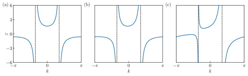
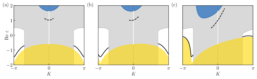
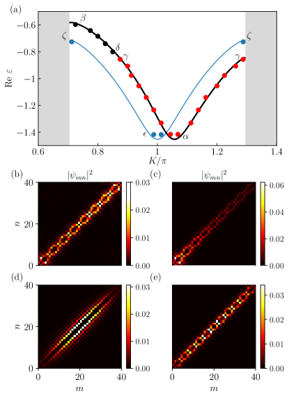
Figure S1 shows the single-photon dispersion branch, calculated for three different values of the chirality parameter using the following equation [34]
| (S1) |
Figure S2(a–c) presents the two-photon dispersion calculated for three different values of . The continuum of the scattering states is obtained by taking the value range of
for varying . The bound states spectra are obtained by numerically diagonalizing Eq. (4) in the main text. The middle panel is the same as the inset in Fig. 2(a) in the main text. The calculation in Figure S2 demonstrates, that the binding energy of the considered bound state dispersion branch decreases for smaller . The branch approaches the continuum of scattering states, corresponding to two polaritons in the lower dispersion branch (yellow area). As a result, the bound state stops being localized. This leads to suppression of the considered NHSE, where the bound state is localized at the “wrong” left edge of the structure for .
II Linear-in-K dispersion terms
In this section, we derive an approximate analytical solution for the linear-in- terms in the bound state dispersion law
| (S2) |
near the center-of-mass Brillouin zone edge .
In an infinite periodic array, the wavefunction that describes the double-excited states can be written as
| (S3) |
The Hamiltonian (2) from the main text then assumes the form
| (S4) | |||
| (S5) |
where is a parameter characterizing the degree of chirality. We can obtain the analytical expressions of the bound state and scattering states at in a non-chiral case [27]:
| (S6) |
where is the inverse effective size of the bound pair and is the wave vector of relative motion of the two particles in a scattering state. The wavefunction of the bound state is normalized as . The bound state and scattering states have the energies
| (S7) |
The linear-in- term, proportional to in Eq. (S2), is induced by the chirality of the Hamultonian. It can be obtained with perturbation theory by considering the first order derivative of the bound state energy at :
| (S8) |
Here, is the first order perturbation to . We remind that the wavefunction amplitudes and are real-valued, and that .
The first term in Eq. (S8) gives:
| (S9) |
The calculation of the second term in Eq. (S8) is also straightforward but relatively cumbersome. At the first step we obtain
| (S10) |
and
| (S11) |
The integral is evaluated as
| (S12) |
Finally, the result reads
| (S13) |
this is equivalent to Eq. (6) in the main text for . In a similar way, we can get the effective mass at zeroth order in [27]:
| (S14) |
III Eigenstates of the effective model
Here, we analyze in more detail the eigenstates of the effective non-Hermitian Hamiltonian Eq. (7) in the main text. In order to verify the exponential character of localization, we have plotted in Fig. S4 the most-localized state, corresponding to the energy values in the center of the band, that is, closest to zero [see Fig. 4 in the main text]. The calculation demonstrates that the wavefunction is not localized at the edge for (red circles). For it is exponentially at the left or right edge depending on the sign of (triangles). The localization length can be estimated by solving the dispersion equation
| (S15) |
for and (as can be inferred from Fig. 4 in the main text ). The result is for . Thin straight lines in Fig. S4 show the corresponding exponential dependences and well describe the overall decay of the numerically calculated eigenmode.
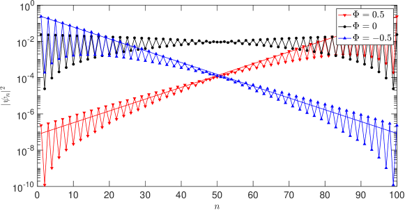
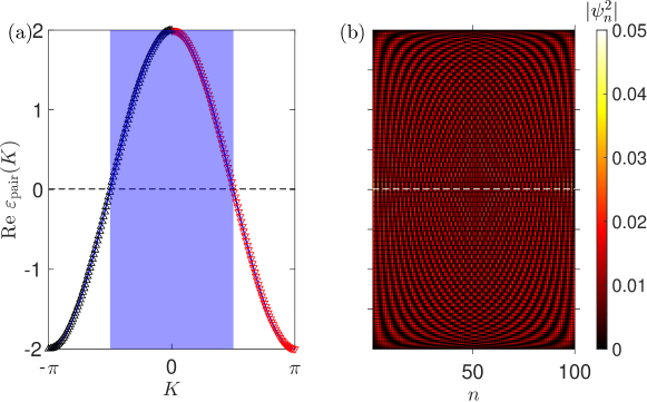
Figure S5 shows the dispersion (a) and the spatial profile (b) for the eigenstates in the effective single-particle model Eq. (7) in the main text. The parameters correspond to Fig. 3 in the main text, but with zero chirality, . As a result, the eigenstates in Fig. S5(b) do not manifest localization at the edge.
To check that the results do not qualitatively depend on and for we present in Fig. S6 the same calculation as in Fig. 4 in the main text, but for and two values of the step smoothness parameter (a) and (b).