MoE²: Optimizing Collaborative Inference
for Edge Large Language Models

Abstract

Large language models (LLMs) have demonstrated remarkable capabilities across a wide range of natural language processing tasks. Exploiting the heterogeneous capabilities of edge LLMs is crucial for diverse emerging applications, as it enables greater cost-effectiveness and reduced latency. In this work, we introduce Mixture-of-Edge-Experts (MoE²), a novel collaborative inference framework for edge LLMs. We formulate the joint gating and expert selection problem to optimize inference performance under energy and latency constraints. Unlike conventional MoE problems, LLM expert selection is significantly more challenging due to the combinatorial nature and the heterogeneity of edge LLMs across various attributes. To this end, we propose a two-level expert selection mechanism through which we uncover an optimality-preserving property of gating parameters across expert selections. This property enables the decomposition of the training and selection processes, significantly reducing complexity. Furthermore, we leverage the objective’s monotonicity and design a discrete monotonic optimization algorithm for optimal expert selection. We implement edge servers with NVIDIA Jetson AGX Orins and NVIDIA RTX 4090 GPUs, and perform extensive experiments. Our results validate that performance improvements of various LLM models and show that our MoE² method can achieve optimal trade-offs among different delay and energy budgets, and outperforms baselines under various system resource constraints.

I Introduction

I-A Background and Motivations

Large language models (LLMs) represent a significant breakthrough in artificial intelligence, particularly in the field of natural language processing (NLP). Built primarily on the transformer architecture [1], LLMs are trained on vast and diverse datasets, enabling them to generate and contextualize human language to a remarkable extent. Prominent examples, such as OpenAI’s GPT series [2, 3] and Google’s PaLM [4, 5, 6], demonstrate the capability of LLMs to perform a wide range of tasks, including text generation, summarization, translation, and question answering. Their versatility stems from their ability to learn and generalize patterns in language, making them indispensable for applications spanning from conversational AI to code generation and beyond. However, this capability comes at the cost of immense computational and memory requirements, as LLMs often contain billions of parameters. This resource-intensive nature creates challenges for their deployment, particularly in environments where computational resources are limited, such as edge devices. As the demand for real-time, localized AI services grows, addressing these challenges has become a critical focus for researchers and practitioners alike.

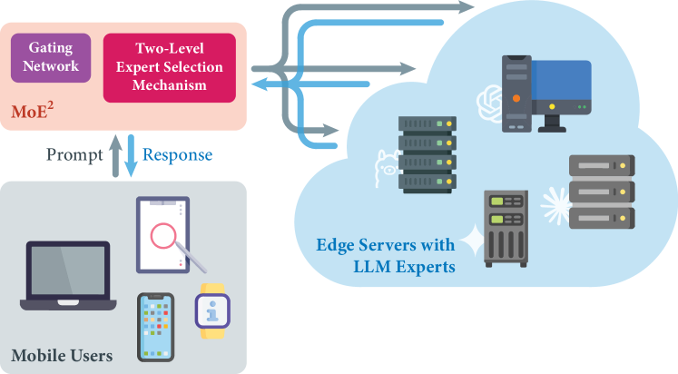
Figure 1: An overview of the MoE² framework, which leverages a gating network and a two-level expert selection mechanism for efficient task processing. Mobile users send prompts, which are routed to a subset of edge servers with LLM experts. The expert selection method is carefully designed to enable a scalable and efficient framework for diverse LLM applications.

On the other hand, the convergence of edge intelligence, mobile edge computing, and LLMs is redefining the landscape of AI-driven applications by enabling powerful computational capabilities closer to end users. Mobile Edge Computing (MEC) is a paradigm that brings computational resources closer to end users by deploying processing power and storage at the edge of mobile networks, while edge intelligence leverages the processing power of edge devices to perform real-time, localized decision-making. However, the deployment of LLMs at the edge is inherently challenging due to their high computational and memory requirements, which often exceed the resource constraints of edge devices. This interplay between edge intelligence, mobile edge computing, and LLMs highlights the need for innovative task offloading techniques to balance performance, resource efficiency, and user experience. Understanding this dynamic is crucial for unlocking the full potential of LLMs in edge settings, enabling applications such as real-time translation, conversational AI, and intelligent assistance to flourish in resource-constrained environments.

In this paper, we aim to bridge this gap by answering the following key question:

Question.

How can collaborative inference leverage heterogeneous edge LLMs to handle diverse task requests (prompts) to balancing performance, latency, and energy consumption?

I-B Key Challenges and Solution Approach

In this work, we propose deploying Mixture-of-Experts (MoE) paradigm at network edges to enable efficient collaborative edge inference. Originally introduced to tackle complex tasks by dividing them into subtasks and assigning them to specialized experts, MoE [7, 8] has evolved into a powerful approach for efficiently up-scaling models through sparse activation [9, 10, 11]. In this sense, MoE is particularly suited for addressing the computational and efficiency challenges posed by large-scale models, such as LLMs. Unlike traditional models, which activate all parameters during inference, MoE dynamically activates a small subset of specialized “expert” submodels for each task [7]. This dynamic routing mechanism significantly scales model capacity without a proportional increase in computational overhead, ensuring high efficiency for resource-intensive tasks. By leveraging only the most relevant experts for a given task, MoE not only achieves better performance but also optimizes resource utilization, such as memory and processing power. MoE’s modular and sparse traits has great potential in reducing training and inference costs for LLMs.

In the context of edge networks, MoE provides a powerful approach for leveraging the heterogeneous capabilities of edge LLM experts by adapting computations to local resource constraints and task-specific requirements. By selecting a subset of edge LLM experts tailored to each inference task, MoE effectively minimizes computational overhead and latency. Furthermore, strategically deploying MoE at the edge enables optimization of LLM performance while reducing energy consumption and latency, thereby enhancing the overall user experience.

However, several key challenges remain, including:

1. Various Attributes across Edges: Traditional MoE approach typically choose experts merely based on gating values. Although this approach may reduce computational overhead, it cannot be deployed directly in networks with edge LLMs that are heterogeneous in various attributes, including capability, energy consumption, and latency.

2. Combinatorial Optimization: To satisfy the system constraints, we proposed an optimization problem to select the optimal subset of LLM experts for each query. However, this problem is challenging due to the expert subset selection’s combinatorial nature, the loss function’s non-convexity, and the complex interplay between system constraints. Traditional optimization techniques may not be suitable to resolve these competing objectives simultaneously.

In this work, we introduce Mixture-of-Edge-Experts (MoE²), a novel collaborative inference framework for edge LLMs, as shown in Fig. 1. Our framework introduces a two-level expert selection mechanism. At the coarse-grained level, the selection is optimization-based, ensuring worst-case bounds on energy consumption and latency. At the fine-grained level, experts are dynamically selected based on input prompts through a routing network. This approach effectively leverages the heterogeneity in the capabilities of edge LLM experts to handle diverse tasks. Our main contributions are summarized as follows:

• MoE Design and Problem Formulation: We formulate the first MoE-aided inference offloading problem for edge LLMs by optimally designing the gating network and expert selection, subject to energy consumption and latency constraints. This problem is inherently combinatorial and challenging due to the heterogeneous nature of edge LLMs.

• Optimal Solution Structures: To address the challenges of combinatorial optimization, we leverage the structural properties of the optimal solution. Specifically, we show that: (i) the optimality of gating parameters for the full LLM set extends to its subsets, and (ii) the objective value exhibits a monotonic improvement property during LLM set selection. These analytical insights demonstrate that the training of gating parameters can be decoupled from the selection of LLM experts, and facilitate our optimization algorithm design.

• Algorithm Design. The MoE² framework, including a training stage and an inference stage, is designed based on two derived theorems. We also propose a cluster-based domain identification method to create domain experts, which efficiently utilizes the strength of our MoE framework.

• Implementation: We implement MoE² on edge servers, and perform extensive experiments. Our results validate that performance improvements of various LLM models and show that MoE² can adapt to different delay and energy budgets with optimal trade-offs, and achieves strong performance compared to baselines under various system resource constraints.

We organize the rest of this paper as follows. Section II presents the literature review. Section III presents the system model and formulates the problem. The proposed scheme is presented in Section IV. Sections V and VI present the simulation and experimental results, respectively. Finally, this paper is concluded in Section VII.

II Related Works

II-A Mobile Edge Computing and Collaborative Inference

In recent years, extensive research has explored MEC across various settings (e.g., [12, 13, 14, 15]). This work primarily reviews the collaborative inference literature in this domain, which focuses on deploying machine learning models at the edge to enable real-time data processing and decision-making [16]. The collaborative inference literature can be categorized into two main approaches: model partitioning and edge-cloud collaboration. In edge-cloud collaboration, edge devices and the cloud cooperate to balance system performance with resource constraints. Time-sensitive tasks are processed locally on edge devices, while more complex or less time-critical workloads are uploaded to the cloud for additional computational support (e.g., [17, 18, 19]). This cooperative mechanism has been leveraged to accelerate inference for large language models (LLMs) [19]. To optimize edge computing, various algorithms have been developed to enable collaborative inference across multiple edge devices, effectively utilizing their combined computational capabilities to enhance model performance (e.g., [20, 21, 22, 23]). Integrating edge computing with AI and edge-cloud collaboration is highly promising for Internet of Things IoT applications requiring low latency, high bandwidth efficiency, and real-time processing [24]. Our proposed MoE² introduces a novel framework for collaborative inference by leveraging the diverse capabilities of LLM experts specialized in handling different tasks, distinguishing it from existing approaches.

II-B Mixture-of-Experts (MoE)

The concept of MoE was first introduced in [7, 8] to dynamically assign inputs to multiple expert networks using a gating network. Early MoE models improved adaptability and accuracy by dividing tasks into sub-tasks, with each expert specializing in specific regions of the input space. The gating network dynamically selects the most relevant experts, enabling efficient problem-solving.

Modern MoE architectures (e.g., [9, 10, 11, 25]), introduced sparse activation, where the gating network activates only a subset of experts for each input, enabling models to scale efficiently to trillions of parameters. Building on this foundation, MoE has recently been applied to address the issue of performance degradation when deploying LLMs on edge devices (e.g., [26, 27]). Our work extends these principles by designing an edge-based MoE system to balance performance, latency, and energy efficiency.

II-C Edge LLMs

The superior performance of LLMs has increasingly captured researchers’ attention, leading to a growing focus on integrating LLMs with edge devices, as recently surveyed in [28].

Edges/Networks for LLMs: Edge deployment of LLMs offers solutions to the challenges of cloud-based systems, such as high latency, data security concerns, and connectivity limitations. By leveraging edge computing, LLMs can process data locally, improving response times, enhancing privacy, and reducing bandwidth usage, which makes them particularly suitable for latency-sensitive and resource-constrained applications [28]. Recent advancements in edge inference techniques for LLMs can be categorized into centralized edge inference, split inference, and collaborative inference. Centralized edge inference reduces communication overhead by optimizing token representations (e.g., [29, 30]) and employing methods such as service placement and migration (e.g., [31, 32, 33, 34]). Split inference divides tasks between edge devices and servers to balance computation and communication, using strategies like token representation reduction (e.g., [35, 36, 37]), progressive offloading [38], early exit [39] and multi-hop architectures [40]. Collaborative inference employs speculative decoding (e.g., [41, 42]), where lightweight models on edge devices generate initial predictions that are refined by powerful servers. These techniques collectively enable scalable and resource-efficient edge inference for LLMs. However, when deploying LLMs at the edge, the trade-offs between performance, latency, and energy efficiency are not always fully considered. In addition, our approach did not require intrusive modifications, i.e., any modifications to edge LLM experts.

LLMs for Edges/Networks: LLMs are transformative in wireless communications, addressing tasks like network configuration, traffic classification, and 6G optimization by reducing human effort and improving efficiency [43]. They are increasingly used for telecom-related tasks, such as domain knowledge generation (e.g., [44, 45]), code generation (e.g., [46, 47, 48, 49]), and network configuration generation (e.g., [50, 51, 52]). LLMs also excel in classification tasks, including network security (e.g., [53, 54, 55, 56, 57]), text (e.g., [58, 59]), image (e.g., [60, 61]), and network traffic classification (e.g., [62, 63]). In network optimization, LLM-enabled techniques like reinforcement learning (e.g., [64, 65, 66]), black-box optimization [67], convex optimization (e.g., [68, 69]), and heuristic algorithms (e.g., [70, 71]) enhance wireless network management. Additionally, LLMs apply time series models like pre-trained foundation models (e.g., [72, 73]), frozen pre-trained models (e.g., [74, 75]), fine-tuning (e.g., [76, 77]), and multi-modality approaches [78] to predict trends and demands. Wu et al. further pioneer LLMs as foundational models for networking with their NetLLM framework, reducing manual efforts and improving adaptability [79]. Our study fundamentally differs from the aforementioned works on “LLMs for networks”, where the primary objective is to utilize LLMs to optimize edge networks, whereas our focus is on leveraging edge resources to support LLMs.

Closely Related Works: Only a couple of studies are closely related. Yi et al. [26] proposed a framework which enables efficient on-device inference with a single LLM on a single edge server, with experts stored in external memory and loaded as needed. This work did not consider collaborative inference by exploiting heterogeneous LLM experts. A concurrent study by Li et al. [80] proposed a MoE model over edges for continual learning, while it did not consider the deployment of large models under a resource-constrained setting.

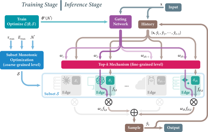
Figure 2: A detailed illustration of the MoE² framework, which consists of training stage and inference stage. In the training stage, the gating network parameters $\bm{\theta}$ are derived by optimizing $\mathcal{L}(\bm{\theta},\mathcal{S})$ over all LLM $\mathcal{N}$. Then, the subset selection $\mathcal{S}$ are obtained by Subset Monotonic Optimization algorithm to satisfy system constraints. In the inference stage, the gating network computes the gating values for each LLM experts, and Top-$k$ mechanism selects a smaller subset from $\mathcal{S}$ of $k$ LLMs with the highest gating values for responding to prompt $\mathbf{x}$.

III System Model and Problem Formulation

In this section, we present the system model for edge LLMs, the MoE² architecture, and the two-level expert selection scheme. We then formulate the joint gating parameter training and LLM expert selection problem.

III-A Edge LLM System Overview

System Overview. As shown in Fig. 2, we consider a system of a set $\mathcal{N}$ of specialized LLM experts (agents). Each LLM expert $n\in\mathcal{N}$ is deployed on one edge server.

Task Model. Mobile users with inference tasks may choose to offload them to edge LLM experts. Let $\mathcal{X}$ represent the set of all prompts requested by different users. Users may send prompts $\mathbf{x}\in\mathcal{X}$ to edge servers based on their specific applications. Future edge LLMs have diverse applications, including mobile health, humanoid robots, virtual assistants, and autonomous driving [28]. For example, Google’s Med-PaLM 2 is an LLM fine-tuned on medical datasets, designed to provide answers to medical inquiries. Beyond this, healthcare LLMs can assist with tasks such as medical question answering, diagnosis, treatment planning, and medical report generation.

We consider a set $\mathcal{M}$ representing categories of LLM applications, which constitute $M$ partitions of $\mathcal{X}$. Specifically, we use $\mathcal{X}_{m}$ to denote the set of prompts (tasks) $\mathbf{x}$ associated with LLM application $m$. Each LLM application has its own latency requirements, which will be specified later.

Autoregressive Process. The system processes $\bm{x}$ and returns $T$ prediction tokens through the autoregressive process. The length $T$ is decided by the experts through the autoregressive process defined as follows. Starting with the prompt $\mathbf{x}$, an LLM agent generates output tokens $\hat{y}_{t}$ at time step $t\in T$ sequentially. The system maintains a history $h(\mathbf{x},t)=\{\mathbf{x},\hat{y}_{1},\cdots,\hat{y}_{t-1}\}$ that combines the original prompt and all previously generated tokens. At time step $t$, an LLM expert $n\in\mathcal{N}$ may processes this history through the LLM output function $f_{n}$ to generate a probability distribution $f_{n}(h(\mathbf{x},t))\in\mathcal{P}(\mathcal{V})$ for the next token $\hat{y}_{t}$, where $\mathcal{V}$ is the used vocabulary space. The generation of $\hat{y}_{t}$ from $f_{n}(h(\mathbf{x},t))$ will be discussed later.

Distributions. Each prompt $\mathbf{x}$ is paired with a target answer $\bm{y}=[y_{t}]_{t=1}^{T}$. We let $\mathcal{P}_{\mathbf{x}}$ be the probability distribution of different prompts, requested by the users, and let $\mathcal{P}_{\mathbf{x},\bm{y}}$ denote the joint distribution of $(\mathbf{x},\bm{y})$. For each LLM application $m\in\mathcal{M}$, we use $\mathcal{P}_{\mathbf{x},m}$ to denote the probability distribution of $\mathbf{x}$ conditioned on $\mathbf{x}\in\mathcal{X}_{m}$.

III-B The Mixture-of-Edge-Experts (MoE²) Architecture

MoE². The system employs an MoE-like architecture to select a subset of edge LLM experts to generate token predictions dynamically. MoE² consists of two key components: a gating network and a two-level expert selection mechanism. Given a prompt $\mathbf{x}$, the generated distributions $f_{n}(h(\mathbf{x},t))$ are weighed by the gating network and aggregated at the user end to generate the final token $\hat{y}_{t}$, which is subsequently added to the history $h(\mathbf{x},t)$ for future generation. This iterative process continues, with each new token generation benefiting from the accumulated context of all previous predictions.

III-B1 Gating Network

Our system implements a distributed architecture where each edge server hosts a dedicated gating network that optimizes the routing weights for the accessible LLM experts. The gating network employs an embedding model to extract textual information and a multi-layer perceptron (MLP) to generate gating values for the LLM experts. Upon receiving a prompt from a mobile user, the nearest edge server processes the request with its gating network, coordinates the token generation process, and synthesizes the final response for transmission back to the user. Let $\bm{\theta}$ denote the gating parameters of the gating network. Given prompt $\mathbf{x}$, the gating network [9] outputs:

$$\mathbf{g}(\mathbf{x},\bm{\theta})=[g_{n}(\mathbf{x},\bm{\theta})]_{n\in\mathcal{N}},$$ (1)

where $g_{n}(\mathbf{x},\bm{\theta})$ is the $n$-th element of $\mathbf{g}(\mathbf{x},\bm{\theta})$. An example gating function $g_{n}(\mathbf{x},\bm{\theta})$ is the multilayer perceptron (MLP). Given the gating values, we compute the weights of experts with different expert selections. Given prompt $\mathbf{x}$, for any select subset of experts $\mathcal{S}\subseteq\mathcal{N}$, we compute the normalized weights of $\mathcal{S}$ as:

$$\bm{\omega}(\mathbf{x},\bm{\theta},\mathcal{S})=\left[\omega_{n}(\mathbf{x},\bm{\theta},\mathcal{S})\right]_{n\in\mathcal{S}}=\left[\frac{g_{n}(\mathbf{x},\bm{\theta})}{\sum\limits_{n^{\prime}\in\mathcal{S}}g_{n^{\prime}}(\mathbf{x},\bm{\theta})}\right]_{n\in\mathcal{S}},$$ (2)

Then, we can obtain the ensemble prediction by a weighted combination of expert outputs [9]. The fused probability distribution of token $k$ is expressed as:

$$F(\mathbf{x},\bm{\theta},\mathcal{S},t)=\sum\limits_{n\in\mathcal{S}}\omega_{n}(\mathbf{x},\bm{\theta},\mathcal{S})f_{n}(h(\mathbf{x},t)).$$ (3)

Note that $F(\mathbf{x},\bm{\theta},\mathcal{S},t)$ is a probability distribution of $\mathcal{V}$, i.e., $F(\mathbf{x},\bm{\theta},\mathcal{S},t)\in\mathcal{P}(\mathcal{V})$. A new token $\hat{y}_{t+1}$ is sampled directly from $F(\mathbf{x},\bm{\theta},\mathcal{S},t)$, i.e., $\hat{y}_{t+1}\sim F(\mathbf{x},\bm{\theta},\mathcal{S},t)$. Then, $\hat{y}_{t+1}$ will be added to the history information $h(\mathbf{x},t+1)$. This process repeats until a stop token is generated.

III-B2 Two-Level Expert Selection Mechanism

One of the key challenges, compared to conventional MoE architectures, lies in the joint selection of LLM experts and the training of gating parameters. Traditional MoEs typically choose experts merely based on gating values, employ additional routing networks to introduce sparsity. These routing networks often add tunable noise and retain only the top $k$ values before applying the softmax function (as in (2)). Although this approach can reduce computational overhead, it cannot be directly deployed in networks with edge LLMs that are heterogeneous across various attributes, including capability, energy consumption, and latency.

To address the above challenge, we propose an LLM expert selection scheme comprising two levels: a coarse-grained level and a fine-grained level, as illustrated in Fig. 2:

• The coarse-grained level selects a subset of LLM experts, denoted by $\mathcal{S}$, based on system constraints, such as through optimization-based methods. This selection ensures a worst-case bound on energy consumption and induced latency, accounting for scenarios where all LLM experts in $\mathcal{S}$ are utilized.

• In the fine-grained level, LLM experts are further selected from the subset $\mathcal{S}$ dynamically based on prompts $\mathbf{x}$ via a routing network, leveraging the heterogeneity of LLM agents in handling different tasks while further reducing system costs.

As we will demonstrate later, the two-level expert selection mechanism, combined with a sufficiently sophisticated gating function $\mathbf{g}(\mathbf{x},\bm{\theta})$, is crucial for enabling efficient algorithm design to jointly train $\bm{\theta}$ and optimize $\mathcal{S}$.

III-B3 Where to Deploy/Train MoE²

Based on our experimental results presented later, a gating network with superior performance can be as small as 1.7GB, enabling its deployment on edge servers (alongside edge LLMs) to serve nearby users effectively. This also opens up the possibility of adopting edge federated learning or cloud-edge collaboration frameworks, where training is conducted in the cloud and deployment occurs at edges.

III-C System Constraints

In reality, LLM applications typically have specific service requirements, which make deploying LLMs at the mobile edge a more efficient solution. The system incurs costs from two primary sources: system delay and energy consumption.

III-C1 System Delay

The system delay in our system can be categorized into three components: the computational time of the LLM experts, the transmission latency between edge devices and mobile devices, and the ensemble time when aggregating the outputs of LLM experts. For an edge LLM agent $n$, the computation time of prompt $\mathbf{x}$ can be represented as:

$$\tau_{n}^{\mathrm{comp}}(\mathbf{x})=\frac{C^{\mathrm{token}}_{n}(\mathbf{x})}{C_{n}^{\mathrm{cap}}}+\frac{M_{\mathrm{size}}}{b_{n}}+C^{\mathrm{ovh}}_{n},$$ (4)

where:

• $C^{\mathrm{token}}_{n}(\mathbf{x})$: Average computational cost per token (in FLOPs) for edge LLM model $n$ for input $\mathbf{x}$.

• $C_{e}^{\mathrm{cap}}$: Computational capability (in FLOPs per second) of edge server $e$.

• $M_{\mathrm{size}}$: Average memory access size (in bytes).

• $b_{n}$: Memory bandwidth (in bytes per second) of edge server $n$.

• $C^{\mathrm{ovh}}_{e}$: Constant overhead for operations, e.g., data transfer between CPU and GPU of edge server $e$, which cannot be overlapped with other operations (in seconds).

The transmission delay between LLM agent $n$ and mobile devices can be calculated as:

$$\tau^{\mathrm{tran}}_{n}(\mathbf{x})=\frac{D(\mathbf{x})}{R_{n}},$$ (5)

where $D(\mathbf{x})$ is the data size of the transmitted prompt $\mathbf{x}$ and $R_{n}(t)$ is the achievable data rate between LLM agent $n$ and users.

For an answer with $T$ tokens, the delay between mobile user $u$ and edge server with LLM model $n$ can be expressed as the followings, where for all $t\in[T]$,

$$\tau_{n}(\mathbf{x},t)= \tau^{\mathrm{comp}}_{n}(h(\mathbf{x},t))+\tau_{u}^{\mathrm{tran}}(\hat{y}_{t-1})+\tau^{\mathrm{tran}}_{n}(p_{n,t}),$$ (6)

where we set $h(\mathbf{x},0)=\mathbf{x}$ and $\hat{y}_{0}=\mathbf{x}$ for simplicity, and define $[T]\triangleq\{1,\cdots,T\}$.

We use $\tau(\mathbf{x},\mathcal{S})$ to denote the overall delay for token-level ensemble generation of prompt $x$ with LLM models subset $\mathcal{S}$, given by:

$$\tau(\mathbf{x},\mathcal{S},t)\triangleq\max\limits_{n\in\mathcal{S}}\{\tau_{n}(\mathbf{x},t)\}.$$ (7)

In other words, the overall delay is determined by the the slowest edge LLM expert within the selected subset $\mathcal{S}$, as the framework cannot generate the next token until all experts have completed their computations. The long-term system delay can be expressed as ($\tau^{\mathrm{gate}}$ is the delay of gating network computation):

$$\tau(\mathbf{x},\mathcal{S})=\frac{1}{T}\sum_{t=1}^{T}\tau(\mathbf{x},\mathcal{S},t)+\tau^{\mathrm{gate}}.$$ (8)

Finally, each LLM application $m\in\mathcal{M}$ has its own latency requirement, given by the following constraint:

$$\mathop{\mathbb{E}}\limits_{\mathbf{x}\sim\mathcal{P}_{\mathbf{x},m}}[\tau(\mathbf{x},\mathcal{S})]\leq\tau_{\max,m},\quad\forall m\in\mathcal{M},$$ (9)

where $\tau_{\max,m}$ is the delay limit (deadline) in response to arbitrary prompt $\mathbf{x}$ for LLM application $m$.

III-C2 System Energy Consumption

The energy consumption of our system mainly depends on the computational energy consumption of inference for edge LLM experts. The total energy consumption for token-level ensemble generation is:

$$E(\mathbf{x},\mathcal{S},t)\triangleq\sum_{n\in\mathcal{S}}E_{n}^{\mathrm{comp}}(h(\mathbf{x},t)),$$ (10)

where $E_{n}^{\mathrm{comp}}(h(\mathbf{x},t))$ represents the energy consumption to inference input $h(\mathbf{x},t)$ for the LLM agent $n$. The long-term system energy consumption can be represented as:

$$E(\mathbf{x},\mathcal{S})=\frac{1}{T}\sum_{t=1}^{T}E(\mathbf{x},\mathcal{S},t),$$ (11)

which is constrained as:

$$\mathop{\mathbb{E}}\limits_{\mathbf{x}\sim\mathcal{P}_{\mathbf{x}}}[E(\mathbf{x},\mathcal{S})]\leq E_{\max},$$ (12)

where $E_{\max}$ is the energy budget.

III-D Problem Formulation

Our objective is to jointly optimize the (coarse-grained level) expert selection $\mathcal{S}$ and train the gating parameters $\mathcal{\bm{\theta}}$, considering the performance of LLM agents under the aforementioned system delay constraints and energy consumption constraint. To measure the quality of the ensemble answer generated by an expert subset $\mathcal{S}$. For an answer with $T$ tokens generated from $\mathcal{S}$, the loss function of the ensemble prediction is defined as:

$$\mathcal{L}(\bm{\theta},\mathcal{S},\mathbf{x},\bm{y})\triangleq-\sum_{t=1}^{T}\log\left(\sum\limits_{n\in\mathcal{S}}\omega_{n}(\mathbf{x},\bm{\theta},\mathcal{S})f_{n,y_{t}}(h(\mathbf{x},t))\right),$$ (13)

where $f_{n,y_{t}}(h(\mathbf{x},t))$ denotes the probability of $y_{t}$ in $f_{n}(h(\mathbf{x},t))$. The expected loss function of the whole distribution can be denoted as:

$$\mathcal{L}_{\rm exp}(\bm{\theta},\mathcal{S})=\mathop{\mathbb{E}}\limits_{(\mathbf{x},\bm{y})\sim\mathcal{P}_{\mathbf{x},\bm{y}}}[\mathcal{L}(\bm{\theta},\mathcal{S},\mathbf{x},\bm{y})].$$ (14)

Since $\mathcal{P}_{\mathbf{x},\bm{y}}$ is not directly accessible in practice, we consider to use an empirical loss function instead:

$$\mathcal{L}(\bm{\theta},\mathcal{S})=\frac{1}{|\mathcal{D}|}\sum_{(\mathbf{x},\bm{y})\in\mathcal{D}}\mathcal{L}(\bm{\theta},\mathcal{S},\mathbf{x},\bm{y}),$$ (15)

where $\mathcal{D}$ is a training dataset. We now formulate the optimization problem:

This problem is challenging due to the combinatorial nature of the expert subset selection, the non-convexity of the loss function, and the complex interplay between the system delay and energy consumption constraints. For a given input, the system must select the optimal subset of experts to minimize the loss function while satisfying the constraints on delay and energy consumption. Traditional optimization techniques may not be suitable for addressing these competing objectives simultaneously. Therefore, we propose a novel methodology to solve this problem effectively and efficiently.

Remark 1.

We note that $\mathcal{P}_{\mathbf{x}}$, which is required in the constraints of (16), is also not directly accessible in practice. However, based on our experimental results presented later, both $\tau(\mathbf{x},\mathcal{S})$ and $E(\mathbf{x},\mathcal{S})$ primarily depend on the length of the prompts, and their statistical significance becomes notable only when the prompt length exceeds $1024$ tokens. This implies that $\mathop{\mathbb{E}}\limits_{\mathbf{x}\sim\mathcal{P}_{\mathbf{x},m}}[\tau(\mathbf{x},\mathcal{S})]$ and $\mathop{\mathbb{E}}\limits_{\mathbf{x}\sim\mathcal{P}_{\mathbf{x}}}[E(\mathbf{x},\mathcal{S})]$ are much easier to estimate in practice compared to $\mathcal{L}_{\exp}(\bm{\theta},\mathcal{S})$.

IV Methodology

MoE² consists of two key stages — training and inference. In training stage, we solve Problem (16) to attain the optimal overall response quality while subject to constraints. While in inference stage, we focus on balancing response quality with system costs.

IV-A Optimal Solution Structures

Define the optimal parameters $\bm{\theta}^{*}$ when fixing the subset $\mathcal{S}$ of edge LLMs:

$$\bm{\theta}^{*}({\mathcal{S}})\triangleq\arg\min\limits_{\bm{\theta}}{\mathcal{L}}(\bm{\theta},\mathcal{S}),\quad\forall\mathcal{S}\subseteq\mathcal{N}.$$ (17)

We provide the theoretical analysis of the relation between $\bm{\theta}$ and $\mathcal{S}$. Then the following theorem extends

Theorem 1 (Optimality for subset).

Let the gating network $\bm{g}(\mathbf{x},\mathcal{\bm{\theta}})$ be an MLP with a sufficiently large width. For any given subset $\mathcal{S}\subseteq\mathcal{N}$ and the optimal parameters satisfy the following condition:

$$\frac{g_{n}(\mathbf{x},\bm{\theta}^{*}({\mathcal{S}}))}{\sum\limits_{n^{\prime}\in\mathcal{S}}g_{n^{\prime}}(\mathbf{x},\bm{\theta}^{*}({\mathcal{S}}))}=\frac{g_{n}(\mathbf{x},\bm{\theta}^{*}({\mathcal{N}}))}{\sum\limits_{n^{\prime}\in\mathcal{S}}g_{n^{\prime}}(\mathbf{x},\bm{\theta}^{*}({\mathcal{N}}))},\forall n\in\mathcal{S}.$$ (18)

The key idea of proving Theorem 1 is conducted by contradiction, constructing a parameter $\bm{\theta}^{\prime}$ through universal approximation that satisfies the required conditions, ultimately leading to a contradiction. For a detailed proof, please refer to Appendix B.

Remark 2.

Theorem 1 indicates that the optimal gating values $\bm{\theta}^{*}(\mathcal{S})$ for any subset $\mathcal{S}$ can be derived directly from the optimal gating values of the complete set $\mathcal{N}$. Consequently, once the optimal parameter $\bm{\theta}^{*}(\mathcal{N})$ for the entire set $\mathcal{N}$ of edge LLMs is obtained, the optimal gating values for any subset $\mathcal{S}$ can be determined without the need for additional training.

Problem (16) can be reduced to a combinatorial optimization over experts as:

$$\min_{\mathcal{S}} \quad\mathcal{L}(\mathcal{\bm{\theta}}^{*}({\mathcal{S}}),\mathcal{S})$$ (19)

s.t. $$\quad\mathop{\mathbb{E}}\limits_{\mathbf{x}\sim\mathcal{P}_{\mathbf{x},m}}[\tau(\mathbf{x},\mathcal{S})]\leq\tau_{\max,m},\quad\forall m\in\mathcal{M},$$

$$\quad\mathop{\mathbb{E}}\limits_{\mathbf{x}\sim\mathcal{P}_{\mathbf{x}}}[E(\mathbf{x},\mathcal{S})]\leq E_{\max},$$

Note that when searching for the optimal $\mathcal{S}^{*}$, Theorem 1 suggests that it is not necessary to repeatedly train the gating networks to obtain $\mathcal{\bm{\theta}}^{*}({\mathcal{S}})$ for each $\mathcal{S}$. This significantly reduces the complexity of the original problem.

Now we aim to optimize subsets $\mathcal{S}$ to satisfy system constraints. We first introduce the property of monotonicity improvement of subsets as follows:

Theorem 2 (Monotonic Improvement).

Let the gating network $\bm{g}(\mathbf{x},\mathcal{\bm{\theta}})$ be an MLP with a sufficiently large width. For any pair of subsets $\mathcal{S},\mathcal{S}^{\prime}\subseteq\mathcal{N}$ such that $\mathcal{S}^{\prime}\subseteq\mathcal{S}$, we have

$$\min_{\bm{\theta}}{\mathcal{L}}(\bm{\theta},\mathcal{S})\leq\min_{\bm{\theta}}{\mathcal{L}}(\bm{\theta},\mathcal{S}^{\prime}).$$ (20)

Proof.

Consider the following function $\bm{f}:\mathcal{X}\rightarrow\mathbb{R}^{|\mathcal{N}|}$, given by

$${f}_{n}(\mathbf{x})=\begin{cases}\frac{g_{n}(\mathbf{x},{\mathcal{\bm{\theta}}}^{*}(\mathcal{S}^{\prime}))}{\sum\limits_{n^{\prime}\in\mathcal{S}^{\prime}}g_{n^{\prime}}(\mathbf{x},\bm{\theta}^{*}({\mathcal{S}^{\prime}}))},&\text{if }n\in\mathcal{S}^{\prime},\\ 0,&\text{if }n\in\mathcal{S}\setminus\mathcal{S}^{\prime},\end{cases}$$ (21)

where $\bm{h}(\mathbf{x})=[{h}_{n}(\mathbf{x})]_{n\in\mathcal{N}}$. Since $\bm{h}(\mathbf{x})$ has at most countably many discontinuities, it is Borel measurable [81]. According to the universal approximation theorem [82], there exists $\hat{\bm{\theta}}$ such that the MLP $\mathbf{g}(\mathbf{x},\hat{\bm{\theta}})$ with a sufficiently large width can approximate $\bm{h}(\mathbf{x})$ to any degree of accuracy.

Then, we have:

$${\mathcal{L}}(\mathcal{\bm{\theta}}^{*}({\mathcal{S}}),\mathcal{S})\leq{\mathcal{L}}(\hat{\bm{\theta}},\mathcal{S})={\mathcal{L}}(\mathcal{\bm{\theta}}^{*}(\mathcal{S}^{\prime}),\mathcal{S}^{\prime}).$$ (22)

∎

IV-B Algorithm Design

We present the algorithm for both training and inference stages.

• The training stage focuses on optimizing the gating network parameters, $\bm{\theta}$, and subset selection to enhance system performance while adhering to system constraints. As suggested by Theorems 1 and 2, the training process for $\bm{\theta}$ can be decoupled from the expert selection process. For the coarse-grained expert selection problem in (16), we propose utilizing the discrete monotonic optimization algorithm [83].

• In the inference stage, the goal is to perform fine-grained subset selection for each query, $\mathbf{x}$, to fully exploit the heterogeneous capabilities of edge LLM experts. The structure of the proposed algorithm is illustrated in Fig. 2.

IV-B1 Training Stage

We first describe the training stage as follows. As shown in Fig. 2, the training stage consists of two sequential steps. First, we utilize Algorithm 1 to obtain parameter $\mathcal{\bm{\theta}}^{*}(\mathcal{N})$ for all LLM agents $\mathcal{N}$, based on the stochastic gradient descent method.

Algorithm 1 Gating Network Training

1: Input: Dataset $\mathcal{D}$ and Batch size $B$ 

2: Output: Optimized parameter $\bm{\theta}^{*}$.

3: while not converged do

4:  Sample a batch $\{\mathbf{x}_{i},\bm{y}_{i}\}_{i\in B}$ from $\mathcal{D}$.

5:  for $i=1,\dots,B$ do

6:   Init $t=0$ and $h(\mathbf{x}_{i},t)=\{\mathbf{x}_{i}\}$.

7:   while true do

8:    Generate gating values $\mathbf{g}(\mathbf{x}_{i},\bm{\theta})$ using the gating network.

9:    Compute normalized weights for all agents $\bm{\omega}(\mathbf{x}_{i},\bm{\theta},\mathcal{N})\leftarrow\left[{g_{n}(\mathbf{x}_{i},\bm{\theta})}\Big{/}{\sum\limits_{n^{\prime}\in\mathcal{\mathcal{N}}}g_{n^{\prime}}(\mathbf{x}_{i},\bm{\theta})}\right]_{n\in\mathcal{N}}$.

10:    Send $\mathbf{x}_{i}$ to all LLM experts and receive $\{f_{n}(h(\mathbf{x}_{i},t)\}_{n\in\mathcal{N}}$.

11:    Fuse the results: $F(\mathbf{x}_{i},\bm{\theta},\mathcal{N},t)\leftarrow\sum\limits_{n\in\mathcal{S}}\omega_{n}(\mathbf{x}_{i},\bm{\theta},\mathcal{N})f_{n}(h(\mathbf{x}_{i},t))$.

12:    Sample next token $\hat{y}_{i,t+1}\sim F(\mathbf{x}_{i},\bm{\theta},\mathcal{N},t)$.

13:    Add $\hat{y}_{i,t+1}$ to history: $h(\mathbf{x},t+1)\leftarrow\{h(\mathbf{x},t),\hat{y}_{i,t+1}\}$,

14:    Accumulate loss: $\mathcal{L}(\bm{\theta},\mathcal{N},\mathbf{x}_{i},\bm{y}_{i})\leftarrow-\log\left(\sum\limits_{n\in\mathcal{S}}\omega_{n}(\mathbf{x}_{i},\bm{\theta},\mathcal{S})f_{n,y_{i,t}}(h(\mathbf{x}_{i},t))\right)$.

15:    if $\hat{y}_{i,t+1}$ is a stop token then

16:     break

17:    end if

18:   end while

19:   Accumulate batch loss $\mathcal{L}(\bm{\theta},\mathcal{N})\leftarrow\mathcal{L}(\bm{\theta},\mathcal{N})+\frac{1}{|\mathcal{D}|}\mathcal{L}(\bm{\theta},\mathcal{N},\mathbf{x}_{i},\bm{y}_{i})$.

20:  end for

21:  Update $\bm{\theta}$: $\bm{\theta}\leftarrow\bm{\theta}+\alpha\partial\mathcal{L}(\bm{\theta},\mathcal{N})/\partial\bm{\theta}$.

22: end while

From Theorem 2, we employ discrete monotonic optimization to address Problem (19). We define $G_{1}$ as the normal hull of the set defined by:

$$G_{1}\triangleq\left\{\mathcal{S}:\mathop{\mathbb{E}}\limits_{\mathbf{x}\sim\mathcal{P}_{\mathbf{x},m}}[\tau(\mathbf{x},\mathcal{S})]\leq\tau_{\max,m},~\forall m\in\mathcal{M}\right\},$$ (23)

and $G_{2}$ as the normal hull of the set defined by:

$$G_{2}\triangleq\left\{\mathcal{S}:\mathop{\mathbb{E}}\limits_{\mathbf{x}\sim\mathcal{P}_{\mathbf{x}}}[E(\mathbf{x},\mathcal{S})]\leq E_{\max}\right\}.$$ (24)

Taking $G$ as their union, i.e., $G=G_{1}\cup G_{2}$, we then define

$$\pi_{G}(\mathcal{S})\triangleq\lambda\mathcal{S},\text{ where }\lambda=\max\{\alpha>0\mid\alpha\mathcal{S}\in G\}.$$ (25)

Now we propose Subset Monotonic Optimization (SMO), as presented in Algorithm 2.

Algorithm 2 Subset Monotonic Optimization (SMO)

1: Initialization: Select tolerance $\varepsilon\geq 0$ and $k\leftarrow 1$ Let $CBV=-\infty$ and $T_{1}=\{\mathcal{N}\}$. 

2: while True do

3:  Step 1:

4:  $\tilde{T}_{k}$ $\leftarrow$ Remove all $\mathcal{S}$ from $T_{k}$ such that $\mathcal{L}(\bm{\theta},\mathcal{S})\geq CBV-\varepsilon$.

5:  Step 2:

6:  if $\tilde{T}_{k}=\emptyset$ then

7:   if $CBV=-\infty$ then

8:    return  Problem (19) is infeasible

9:   else

10:    return  Current best feasible solution $\bar{\mathcal{S}}_{k}$ as an $\varepsilon$-optimal solution.

11:   end if

12:  end if

13:  Step 3:

14:  Select $\mathcal{S}_{k}\in\arg\max\{\mathcal{L}(\bm{\theta},\mathcal{S})|\mathcal{S}\in\tilde{T}_{k}\}$

15:  Compute $\mathcal{S}^{\prime}_{k}=\pi_{G}(\mathcal{S}_{k})$

16:  if $\mathcal{S}^{\prime}_{k}=\mathcal{S}_{k}$ then

17:   return  $\mathcal{S}_{k}$ as an optimal solution.

18:  else

19:   Update new best feasible solution as $\mathcal{S}^{\prime}_{k+1}$ and $CBV=\mathcal{L}(\bm{\theta},\mathcal{S}^{\prime}_{k+1})$.

20:  end if

21:  Step 4:

22:  $V_{k+1}\leftarrow(\tilde{T}_{k}\setminus\{\mathcal{S}_{k}\})\cup\{\mathcal{S}_{k}-(\mathcal{S}_{k}^{i}-\mathcal{S}_{k}^{{}^{\prime}i})e^{i},i=1,\ldots,n\}$

23:  for $\mathcal{S}\in T_{k}\setminus\{\mathcal{S}_{k}\}$ do

24:   for $i=1$ to $n$ do

25:    if $\mathcal{S}\geq\mathcal{S}^{\prime}_{k}$ while $\mathcal{S}_{i}<\mathcal{S}_{k}$ then

26:     Remove $\mathcal{S}_{k}^{i}$ from $V_{k+1}$.

27:    end if

28:   end for

29:  end for

30:  $T_{k+1}\leftarrow V_{k+1}$

31:  Step 5:

32:  Set $k\leftarrow k+1$.

33: end while

Let $CBV$ denote the current best value, $e^{i}$ denote the $i$-th unit vector of the considered space, and $T_{k}$ be the proper vertex set of $\mathcal{N}$. First, we set the tolerance $\varepsilon$ and initialize the iteration counter $k$. The initial vertex set $T_{1}$ is initialized as the complete set of experts $\mathcal{N}$. In each iteration, we remove the subsets with loss values greater than the current best value $CBV-\varepsilon$ from the vertex set $T_{k}$. We then compute the remaining set $\tilde{T}_{k}$. If $\tilde{T}_{k}$ is empty, we check if the problem is infeasible and return the current best feasible solution $\bar{\mathcal{S}}_{k}$. Otherwise, we select the subset $\mathcal{S}_{k}$ with the maximum loss value from the remaining set $\tilde{T}_{k}$. We then compute the projection $\mathcal{S}^{\prime}_{k}$ of $\mathcal{S}_{k}$ onto the feasible region $G$. If $\mathcal{S}^{\prime}_{k}$ is equal to $\mathcal{S}_{k}$, we return $\mathcal{S}_{k}$ as the optimal solution. Otherwise, we update the current best feasible solution as $\mathcal{S}^{\prime}_{k+1}$ and $CBV$ as the loss value of $\mathcal{S}^{\prime}_{k+1}$. We then update the vertex set $T_{k+1}$ by removing $\mathcal{S}_{k}$ and adding the new subsets generated by the vertex $\mathcal{S}_{k}$.

IV-B2 Inference Stage

Now we describe the inference stage. In this stage, we aim to compute the optimal subset selection for each query and generate the answer, which is represented in Algorithm 3.

Algorithm 3 Inference Stage

1: Input: Prompt $\mathbf{x}$ and Optimal subset $\mathcal{S}$ and gating parameters $\bm{\theta}^{*}$.

2: Output: Answer $\hat{\bm{y}}$

3: Calculate gating values $g_{s_{n}}(\mathbf{x},\bm{\theta}^{*})$ for $\mathcal{S}=\{s_{1},s_{2},\dots,s_{n},\dots\}$.

4: Sort $\mathcal{S}$ according to the gating values: $\hat{\mathcal{S}}(\mathbf{x},\bm{\theta}^{*})=\{s_{n}|g_{s_{n-1}}(\mathbf{x},\bm{\theta}^{*})\geq g_{s_{n}}(\mathbf{x},\bm{\theta}^{*})\}$.

5: Select Top-$k$ experts $\Gamma(\mathbf{x},\bm{\theta}^{*},\mathcal{S},k)\leftarrow\{\hat{s}_{1},\hat{s}_{2},\dots,\hat{s}_{k}\}$ where $\hat{s}_{k}\in\hat{\mathcal{S}}(\mathbf{x},\bm{\theta}^{*})$.

6: Compute weights for the selected experts: $\bm{\omega}_{n}(\mathbf{x},\bm{\theta}^{*},\mathcal{S},k)\leftarrow{g_{n}(\mathbf{x},\bm{\theta}^{*})}\big{/}{\sum\limits_{n^{\prime}\in\Gamma(\mathbf{x},\bm{\theta}^{*},\mathcal{S},k)}g_{n^{\prime}}(\mathbf{x},\bm{\theta}^{*})}$.

7: Init $t\leftarrow 0$.

8: while true do

9:  Fuse results: $F(\mathbf{x},\bm{\theta}^{*},\mathcal{S},k,t)\leftarrow$  $\sum\limits_{n\in\Gamma(\mathbf{x},\bm{\theta}^{*},\mathcal{S},k)}\bm{\omega}_{n}(\mathbf{x},\bm{\theta}^{*},\mathcal{S},k)f_{n}(h(\mathbf{x},t))$.

10:  Sample $\hat{y}_{t+1}\sim F(\mathbf{x},\bm{\theta}^{*},\mathcal{S},k,t)$.

11:  Collect answer $\hat{\bm{y}}\leftarrow\hat{y}_{t}$.

12:  if $\hat{y}_{t}$ is a stop token then

13:   return

14:  end if

15: end while

From Theorem 1, we know that the optimal gating values for the subset can be directly obtained from the global optimal gating values, which corresponds to the first step of the inference stage.

Top-$k$ Mechanism. To further reduce system costs while preserving response quality, we employ the Top-$k$ mechanism [9] to select a subset of $k$ LLM experts with the highest gating values from subset $\mathcal{S}$. Specifically, given optimized parameter $\bm{\theta}^{*}$ and prompt $\mathbf{x}$, we first sort all elements in subset $\mathcal{S}$ in ascending order with respect to gating values:

$$\hat{\mathcal{S}}(\mathbf{x},\bm{\theta}^{*})= \{s_{n}\mid g_{s_{n-1}}(\mathbf{x},\bm{\theta}^{*})\geq g_{s_{n}}(\mathbf{x},\bm{\theta}^{*})\},$$ (26)

$$n\in\{1,2,\dots,|\mathcal{S}|\},$$

where $s_{n}\in\mathcal{S}$ is the $n$-th element of $\mathcal{S}$. Then the selected Top-$k$ experts can be denoted as:

$$\Gamma(\mathbf{x},\bm{\theta}^{*},\mathcal{S},k)=\{\hat{s}_{1},\hat{s}_{2},\dots,\hat{s}_{k}\},s_{k}\in\hat{\mathcal{S}}(\mathbf{x},\bm{\theta}^{*}).$$ (27)

Then we can compute the optimal weights for these $k$ LLM experts. For each expert $n\in\Gamma(\mathbf{x},\bm{\theta}^{*},\mathcal{S},k)$ , we have:

$$\bm{\omega}_{n}(\mathbf{x},\bm{\theta}^{*},\mathcal{S},k)=\frac{g_{n}(\mathbf{x},\bm{\theta}^{*})}{\sum\limits_{n^{\prime}\in\Gamma(\mathbf{x},\bm{\theta}^{*},\mathcal{S},k)}g_{n^{\prime}}(\mathbf{x},\bm{\theta}^{*})}.$$ (28)

To generate an answer, we fuse the outputs of the selected experts by a weighted combination as:

$$F(\mathbf{x},\bm{\theta}^{*},\mathcal{S},k,t)=\sum\limits_{n\in\Gamma(\mathbf{x},\bm{\theta}^{*},\mathcal{S},k)}\omega_{n}(\mathbf{x},\bm{\theta}^{*},\mathcal{S},k)f_{n}(h(\mathbf{x},t)).$$ (29)

Then we sample the next token $\hat{y}_{t+1}$ from $F(\mathbf{x},\bm{\theta}^{*},\mathcal{S},k,t)$, i.e., $\hat{y}_{t+1}\sim F(\mathbf{x},\bm{\theta}^{*},\mathcal{S},k,t)$. The process repeats until a stop token is generated.

V Simulation Results

In this section, we deploy MoE² on local devices and test the model performance. We use a novel cluster-based method to create domain experts, which exploits the strength of the MoE mechanism.

V-A Cluster-based Domain Experts

To utilize the strengths of the MoE mechanism, experts are expected to be diverse and specialized in different tasks. However, it is challenging to acquire domain-specific experts due to the following reasons:

• Comprehensive LLM training: Most existing LLM models are trained over diverse datasets, making it difficult to identify domain-specific experts. Although some models are fine-tuned on math or code-related tasks, they may not be sufficient for all tasks.

• Undistinguishable domains: The domain of a given prompt is not always clear, and the prompt may contain multiple domains. For example, should we consider a math question and a physics question as two separate domains or as a single domain?

• Limited domain-specific datasets: It is challenging to collect sufficient domain-specific data to train an expert even if the domain is distinguishable for prompts. To train a domain-specific expert, we need to label a large number of samples, which is time-consuming and expensive.

Therefore, we propose a cluster-based method to create domain-specific datasets from any existing datasets without manual labeling. Our main idea is to cluster the prompts based on their embedding similarity and fine-tune the LLM model on each cluster to create domain-specific experts. Specifically, we use the pre-trained mGTE model [84] to encode the prompts into embeddings, and apply $K$-means algorithm to cluster prompts based on their embeddings. In our simulation, we set $K=8$ for 8 clusters. Finally, we fine-tune the LLM model on each cluster to create domain-specific experts. Other details can be found in Appendix A.

V-B Environment Setup

We evaluate the performance of MoE² in a simulated environment. We construct a system with $N=8$ edge servers, each hosting an LLM agent. We pick Qwen2.5-3B-Instruct [85], Qwen2.5-7B-Instruct [85], Llama-3.2-3B-Instruct [86] and Mistral-7B-Instruct-v0.3 [87] as base models. These LLM agents are duplicated and fine-tuned on each cluster to create domain-specific experts. The gating network is implemented as an MLP with two hidden layers.

We choose MMLU [88] as the evaluation dataset, which is not involved in the fine-tuning process of the LLMs. More details on the fine-tuning process can be found in Appendix A. We retain $80\%$ data in MMLU as the training set for training the gating network, while the other $20\%$ are used as the testing set for the evaluating MoE²’s performance. Other detailed settings are listed in the Appendix A.

V-C Simulation Results

Here, we present the numerical results of MoE². We first evaluate the responsive accuracy of our model compared to the following baselines:

• Single Agent (S. A.): This method evaluates each original model.

• Majority Voting (M. V.): This method assigns equal weights to all fine-tuned LLM agents and fuses the outputs by majority voting. The gating network is not used in this method.

• Average Expert Accuracy (A. E. A.): This metric calculates the average accuracy of each fine-tuned LLM agent on the test set. It reflects the average performance of experts.

Each model’s responsive accuarcy on the MMLU dataset are shown in Fig. 3.

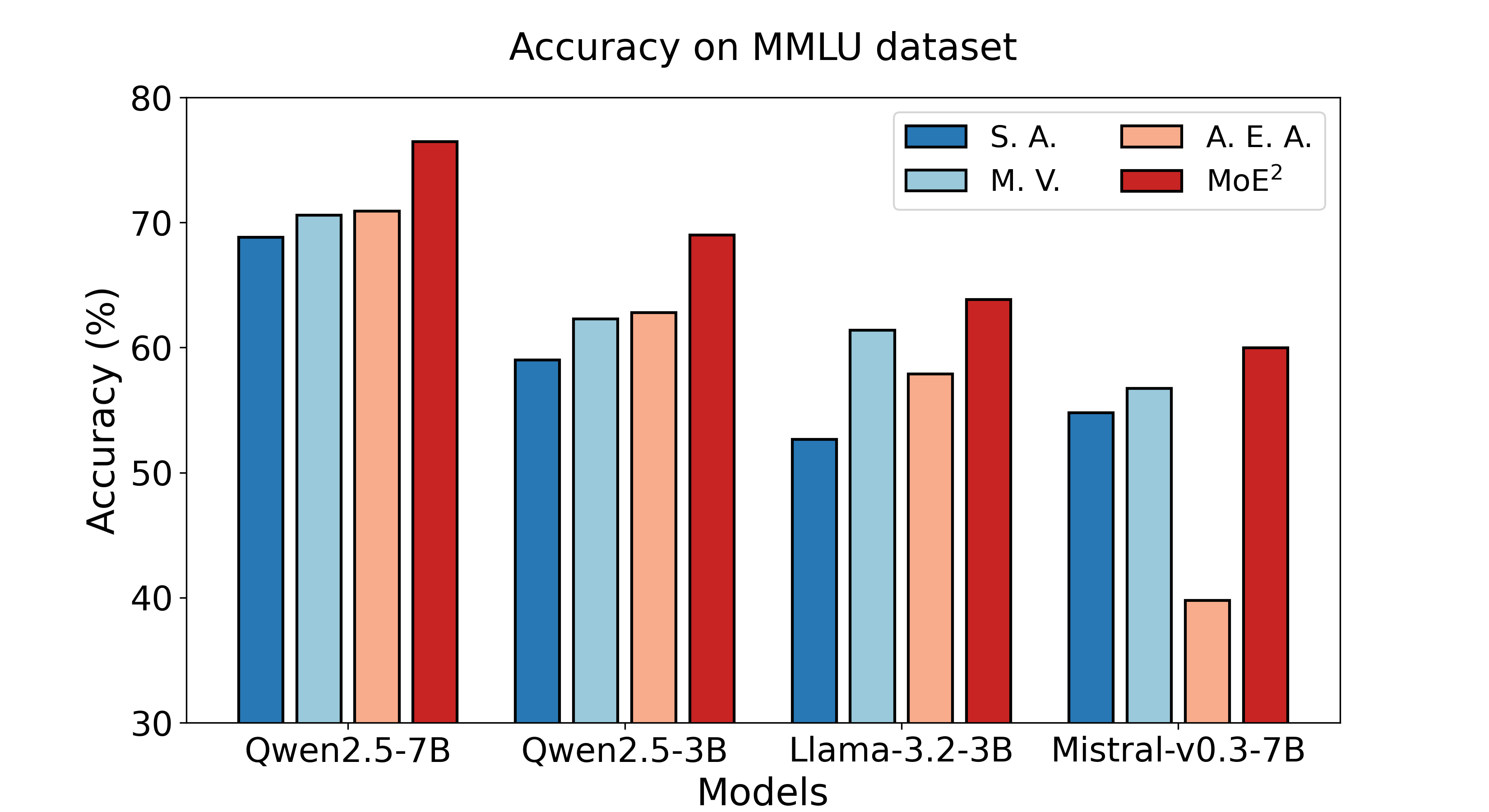
Figure 3: Performance comparison on the MMLU dataset. The MoE² architecture achieves the highest accuracy, which outperforms the Single Agent, Majority Voting and A. E. A. by $14.4\%$, $7.3\%$, $16.4\%$, respectively.

We observe that the MoE² architecture achieves the highest accuracy, outperforming the Single Agent, Majority Voting, and A.E.A. by 14.4%, 7.3%, and 16.4%, respectively. This validates that MoE² significantly enhances the performance of various LLM models.

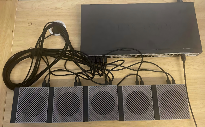
Figure 4: Implementation of an edge LLM testbed on NVIDIA Jetson AGX Orin 64GB, connected to NVIDIA GeForce RTX 4090 via a local area network.

VI Experiment Results

In this section, we implement our MoE² model on developed testbeds as shown in 4. We evaluate its performance under various system constraints.

(a) Edge Delays under Different Prompt Lengths.

(b) Edge Energy Consumptions under Different Prompt Lengths.

Figure 5: Studies of edge delays and edge energy consumptions under different prompt lengths. Edges equipped with less powerful computational resources and larger-scale LLM models exhibit higher delays, while edges equipped with more powerful computational resources and larger-scale LLM models exhibit higher energy consumption.

VI-A Deployment of Edge Devices

TABLE I: Edge Servers Deployment

Index	LLMs	Edge Devices
0	Qwen2.5-7B-FT0-Q4	NVIDIA GeForce RTX 4090
1	Qwen2.5-7B-FT1-Q4	NVIDIA GeForce RTX 4090
2	Qwen2.5-7B-FT2-Q4	NVIDIA Jetson AGX Orin 64GB
3	Qwen2.5-3B-FT3-Q4	NVIDIA GeForce RTX 4090
4	Qwen2.5-3B-FT4-Q4	NVIDIA Jetson AGX Orin 64GB
5	Qwen2.5-3B-FT5-Q4	NVIDIA Jetson AGX Orin 64GB
6	Qwen2.5-3B-FT6-Q4	NVIDIA Jetson AGX Orin 64GB
7	Qwen2.5-3B-FT7-Q4	NVIDIA Jetson AGX Orin 64GB

We implement MoE² on an edge LLM testbed with $N=8$ edge servers, each hosting an LLM agent. The edge servers are named according to the index of domain experts. The deployment details of these edge servers are summarized in Table I. Specifically, edge servers 0, 1, and 2 are deployed on high-performance platforms (NVIDIA GeForce RTX 4090), while the remaining edge servers (3, 4, 5, 6, 7) are deployed on NVIDIA Jetson AGX Orin 64GB devices, as shown in Fig. 4.

We utilize two base LLM models in our deployment: Qwen2.5-7B [85] and Qwen2.5-3B [85]. These models are duplicated and fine-tuned individually before deployment on edge devices, as in Section V. To optimize memory usage and inference latency for edge deployment, we apply 4-bit quantization to the models. For example, “Qwen2.5-7B-FT0-Q4” indicates the Qwen2.5-7B model fine-tuned for cluster 0 and deployed with 4-bit quantization.

VI-B Experiment Results

We first analyze the edge delays and energy consumptions across different servers under varying prompt lengths. As illustrated in Fig. 5, edge servers 0 and 1 with more powerful platforms (NVIDIA RTX 4090) demonstrate significantly lower latency and higher energy consumption compared with edge server 2 with same scale LLM models. Edge server 4-7 equipped with smaller-scale LLM models (3B) exhibits lower delay and energy consumption compared to edge servers 2 with the same platform. Furthermore, Fig. 5 reveals that the edge delays and energy consumptions primarily depend on the length of the prompts. In addition, their statistical significance becomes notable only when the prompt length exceeds $1024$ tokens. This finding indicates minimal variation in processing delays between original prompts and historical context information.

Subsequently, we conduct LLM inference experiments in our collaborative inference framework for edge LLM models. Here we aim to test the model performance under the variation of delay and cost constraints. We evaluate our MoE² framework with the proposed SMO subset selection algorithm and Top-$k$ selection mechanism on various constraints of end-to-end delay $\tau_{\max}$ and energy consumption $E_{\max}$. The baselines are as follows:

• SMO with Majority Voting (SMO M. V. ): This method assigns equal weights to LLM models selected by the proposed SMO selection mechanism.

• Random Subset Selection with Majority Voting (Rand. M. V. ): This method assigns equal weights to LLM models with randomly selected subsets.

TABLE II: Accuracy Comparison for $\tau_{\max}$ = 1 sec

$\mathbf{E_{\max}(J)}$	5	10	15	20	25	35	50
MoE2	58.3	59.3	59.3	59.3	59.3	59.9	59.9
SMO M. V.	58.3	59.1	59.1	59.1	59.1	59.4	59.4
Rand. M. V.	57.5	58.9	56.8	56.1	57.0	59.0	57.5

TABLE III: Accuracy Comparison for $\tau_{\max}$ = 2 sec

$\mathbf{E_{\max}(J)}$	5	10	15	20	25	35	50
MoE2	58.3	59.4	59.4	66.1	71.6	71.7	71.8
SMO M. V.	58.3	59.0	59.2	64.7	71.6	69.5	69.5
Rand. M. V.	58.0	58.4	58.6	58.4	60.4	61.2	63.3

TABLE IV: Accuracy Comparison for $\tau_{\max}$ = 3 sec

$\mathbf{E_{\max}(J)}$	5	10	15	20	25	35	50
MoE2	58.3	66.2	66.2	66.2	71.6	71.7	71.8
SMO M. V.	58.3	66.2	66.2	66.2	71.6	69.5	69.5
Rand. M. V.	58.0	61.5	61.0	60.2	60.7	62.6	62.9

The testbed experiment results are shown in Table II, III, and IV. From Table II, we observe that both MoE² and SMO M. V. consistently outperform Rand. M.V. across all energy constraints under the tightest delay constraint of 1s, demonstrating the effect of the proposed SMO algorithm. In addition, MoE² demonstrates strong performance at higher energy constraints, achieving a 4.2% improvement over Rand. M.V. at energy constraints of 50J per prompt. This indicates that MoE² can effectively utilize the increased energy budget to activate a more optimal set of experts. With a more relaxed delay constraint of 2s in Table III, MoE² outperforms SMO M. V. by an average of 1.38% and Rand. M. V. by an average of 9.4%. The substantial improvements over Rand. M. V. highlights the effectiveness of the MoE² framework in utilizing the increased flexibility to select a more optimal set of experts with the proposed SMO algorithm. With the most relaxed delay constraint shown in Table IV, MoE² demonstrates its ability to effectively utilize the added time flexibility. While it performs on par with SMO M. V. in lower and mid-range energy constraints, it significantly outperforms Rand. M. V. up to 18.0% at 25J. With the increased energy budget (35J and 50J), MoE² surpasses SMO M. V. by 3.2% and 3.3% respectively. This shows the effectiveness of the MoE² framework in utilizing the selected LLM subsets with gating networks at overall relaxed resource constraints.

In summary, the results across all three tables strongly support the effectiveness of the proposed MoE² framework. MoE² consistently outperforms both the SMO M. V. and Random M. V. methods, particularly as the energy constraint $E_{\max}$ increases and the delay constraint $\tau_{\max}$ is relaxed. This highlights the effectiveness of MoE² and the SMO selection mechanism in optimizing the utilization of multiple LLM models on edge devices. The significant improvement over Rand. M.V. underscores the importance of intelligent expert selection. While the improvement over M.V. might seem modest in some cases, it is important to remember that M.V. itself is a strong baseline equipped with proposed SMO subset selection. These findings firmly establish MoE² as a highly promising solution for deploying LLMs in resource-constrained edge computing environments.

VII Conclusions

In this paper, we propose the first MoE-aided collaborative inference framework for edge LLMs by optimally designing the gating network and the two-level expert selection mechanism. Through theoretical analysis, we have proven that the optimality of gating parameters for the entire LLM sets can be extended to any subset, based on which we develop the MoE² framework with SMO. Extensive experiments on real hardware platforms demonstrate that our proposed MoE² framework achieves superior performance compared to baseline methods under diverse system cost constraints. Overall, by leveraging collaborative inference and optimized resource allocation, MoE² paves the way for efficient and effective small-scale LLMs applications in resource-constrained edge computing scenarios.

As the first work in this domain, there are several promising directions for future research. First, it would be valuable to adapt MoE² to dynamic system conditions, such as fluctuating user requests and varying edge server loads. Second, further exploration into edge learning and cloud-edge deployment of MoE² could enhance its practical applicability. Third, the deployment of multi-modal LLMs on edge servers presents an exciting avenue for investigation, along with exploring the potential of MoE² to support LLM agents without requiring fine-tuning.

Figure 6: Clustering Result of MMLU. The prompts are clustered based on their embedding. The results show that similar subjects fall into one cluster. For example, cluster 4 mainly contains math-related and physical-related subjects and cluster 7 includes medical-related subjects. This result coincides with the intuition of us to distinguish domains.

Appendix A Environment Setup

Fine-tuning LLM Agents. We fine-tune the LLM agents using eight NVIDIA Tesla A800 80G GPUs for each cluster to develop domain-specific experts. The steps are as follows:

1. Dataset Fusing. We combine the datasets of different domains to create a comprehensive dataset, including MMLU-pro [89], ARC [90], SciQ [91] and AGIEval [92]. The MMLU dataset is not included in this comprehensive dataset, as it is used for performance evaluation.

2. Embedding-based Clustering. We use the pre-trained mGTE model [84] to encode the prompts into embeddings. Then, we apply the $K$-means algorithm to cluster the prompts based on their embeddings. We set the number of clusters to $8$, corresponding to the number of edge servers in the testbed described in Section VI.

3. Model Fine-tuning. We fine-tune the LLM model on each cluster to create domain-specific experts. We use LoRA [93] method to fine-tune the LLM model. The fine-tuning parameters are shown in Table V.

TABLE V: Fine-tuning Parameters

Parameters	Values
LoRA Rank	$256$
LoRA Alpha	$512$
LoRA Dropout	$0.05$
Cutoff Length	$8192$
Training Epochs	$3$
Batch Size	$8$
Gradient Accumulation Steps	$16$
Optimizer	AdamW
Learning Rate Scheduler	CosineAnnealingLR
Init Learning Rate	$5\times 10^{-5}$
Max Gradient Norm	$1.0$

After fine-tuning, we obtain $8$ domain-specific experts, each corresponding to a cluster. We use these experts as the LLM agents in the MoE system. To validate the effectiveness of this method, we calculate the embeddings of the MMLU dataset and present the clustering results in Fig. 6. From the results, we observe that similar subjects fall into one cluster. For example, cluster 4 mainly contains math-related and physical-related subjects and cluster 7 includes medical-related subjects. This result coincides with the intuition of us to distinguish domains. Most importantly, the dataset used to fine-tune the LLM agents does not include the MMLU dataset, which exhibits strong generalization ability of this clustering method.

Training Gating Network. For the gating network, we use a feed-forward neural network with two hidden layers. We also use a residual connection between the input of each layer and the input of the last layer. All residual activations are concatenated before the final output layer. The learning rate is scheduled by the ReduceLROnPlateau method, which reduces the learning rate by a factor if the validation loss does not improve for a certain number of steps. The parameters of the gating network are shown in Table VI.

Collaborative Inference Architecture. We conduct collaborative inference with edge servers with Nvidia RTX 4090 GPUs and Nvidia Jetson AGX Orins. Detailed configuration is presented in Table I.

TABLE VI: Gating Network Parameters

Parameters	Values
Input (Embedding) Dimension	$1024$
Hidden Dimension	$128$
Output Dimension	$8$
Dropout	$0.1$
Activation Function	PReLU
Optimizer	AdamW
Learning Rate Scheduler	ReduceLROnPlateau
Init Learning Rate	$10^{-5}$
Learning Rate Decay Factor	$0.8$
Learning Rate Decay Patience	$50$
Gradient Clip	$1.0$
Gradient Accumulation Steps	$8$
Batch Size	$8$

Appendix B Proof of Theorem 1

We prove this theorem by contradiction. Suppose that the above theorem does not hold, then there exists an optimal $\hat{\bm{\theta}}$ on $\mathcal{S}$ such that:

$$\mathcal{L}(\hat{\bm{\theta}},\mathcal{S})<\mathcal{L}(\bm{\theta}^{*}(\mathcal{N}),\mathcal{S}).$$ (30)

where $\bm{\theta}^{*}(\mathcal{N})$ satisfies

$$\frac{g_{n}(\mathbf{x},\bm{\theta}^{*}({\mathcal{S}}))}{\sum\limits_{n^{\prime}\in\mathcal{S}}g_{n^{\prime}}(\mathbf{x},\bm{\theta}^{*}({\mathcal{S}}))}=\frac{g_{n}(\mathbf{x},\bm{\theta}^{*}({\mathcal{N}}))}{\sum\limits_{n^{\prime}\in\mathcal{S}}g_{n^{\prime}}(\mathbf{x},\bm{\theta}^{*}({\mathcal{N}}))},\forall n\in\mathcal{S}.$$ (31)

This means that there exists a parameter $\hat{\bm{\theta}}$ that achieves a lower loss on the subset $\mathcal{S}$ compared to $\bm{\theta}^{*}(\mathcal{N})$.

Let $c(\mathbf{x})={\sum\limits_{n\in\mathcal{S}}g_{n}(\mathbf{x},\bm{\theta}^{*}(\mathcal{N}))}\big{/}{\sum\limits_{n\in\mathcal{S}}g_{n}(\mathbf{x},\hat{\bm{\theta}})}$. Consider the function $\bm{h}:\mathcal{X}\rightarrow\mathbb{R}^{|\mathcal{N}|}$, given by

$${h}_{n}(\mathbf{x})=\begin{cases}c(\mathbf{x})g_{n}(\mathbf{x},\hat{\bm{\theta}}),&n\in\mathcal{S},\\ g_{n}(\mathbf{x},\bm{\theta}^{*}(\mathcal{N})),&n\in\mathcal{N}\setminus\mathcal{S},\end{cases}$$ (32)

Since $\bm{h}(\mathbf{x})$ has at most countably many discontinuities, it is Borel measurable [81]. Invoking the universal approximation theorem [82], there exists $\bm{\theta}^{\prime}$ such that the MLP $\mathbf{g}(\mathbf{x},\bm{\theta}^{\prime})$ with a sufficiently large width can approximate $\bm{h}(\mathbf{x})$ to any degree of accuracy.

This which ensures that

$$\sum\limits_{n\in\mathcal{S}}g_{n}(\mathbf{x},\bm{\theta}^{\prime})=\sum\limits_{n\in\mathcal{S}}g_{n}(\mathbf{x},\bm{\theta}^{*}(\mathcal{N})),\forall\mathbf{x}\in\mathcal{X}.$$ (33)

Thus, for all $\mathbf{x}\in\mathcal{X}$, we have

$$\frac{c(\mathbf{x})g_{n}(\mathbf{x},\hat{\bm{\theta}})}{\sum\limits_{n^{\prime}\in\mathcal{S}}c(\mathbf{x})g_{n^{\prime}}(\mathbf{x},\hat{\bm{\theta}})}=\frac{g_{n}(\mathbf{x},\hat{\bm{\theta}})}{\sum\limits_{n^{\prime}\in\mathcal{S}}g_{n^{\prime}}(\mathbf{x},\hat{\bm{\theta}})}.$$ (34)

From the definition of $\mathcal{L}(\bm{\theta},\mathcal{S})$, we have:

$$\mathcal{L}(\hat{\bm{\theta}},\mathcal{S})=\mathcal{L}(\bm{\theta}^{\prime},\mathcal{S})$$ (35)

$$=\frac{1}{|\mathcal{D}|}\sum_{(\mathbf{x},\bm{y})\in\mathcal{D}}\left[\sum_{t=1}^{T}-\left(\log\left(\sum\limits_{n\in\mathcal{S}}g_{n}(\mathbf{x},\bm{\theta}^{\prime})f_{n,y_{t}}(h(\mathbf{x},t))\right)-\right.\right.$$

$$\quad\quad\quad\left.\left.\log\left(\sum\limits_{n^{\prime}\in\mathcal{S}}g_{n^{\prime}}(\mathbf{x},\bm{\theta}^{\prime})\right)\right)\right]$$

$$<\mathcal{L}(\bm{\theta}^{*}(\mathcal{N}),\mathcal{S})$$

$$=\frac{1}{|\mathcal{D}|}\sum_{(\mathbf{x},\bm{y})\in\mathcal{D}}\left[\sum_{t=1}^{T}-\log\left(\sum\limits_{n\in\mathcal{S}}\frac{g_{n}(\mathbf{x},\bm{\theta}^{*}(\mathcal{N}))}{\sum\limits_{n^{\prime}\in\mathcal{S}}g_{n^{\prime}}(\mathbf{x},\bm{\theta}^{*}(\mathcal{N}))}f_{n,y_{t}}(h(\mathbf{x},t))\right)\right]$$

$$=\frac{1}{|\mathcal{D}|}\sum_{(\mathbf{x},\bm{y})\in\mathcal{D}}\left[\sum_{t=1}^{T}-\left(\log\left(\sum\limits_{n\in\mathcal{S}}g_{n}(\mathbf{x},\bm{\theta}^{*}(\mathcal{N}))f_{n,y_{t}}(h(\mathbf{x},t))\right)\right.\right.$$

$$\quad\quad\quad\left.\left.-\log\left(\sum\limits_{n^{\prime}\in\mathcal{S}}g_{n^{\prime}}(\mathbf{x},\bm{\theta}^{*}(\mathcal{N}))\right)\right)\right].$$

From (33), it follows

$$\frac{1}{|\mathcal{D}|}\sum_{(\mathbf{x},\bm{y})\in\mathcal{D}}\left[\sum_{t=1}^{T}-\log\left(\sum\limits_{n\in\mathcal{S}}g_{n}(\mathbf{x},\hat{\bm{\theta}})f_{n,y_{t}}(h(\mathbf{x},t))\right)\right]$$ (36)

$$<\frac{1}{|\mathcal{D}|}\sum_{(\mathbf{x},\bm{y})\in\mathcal{D}}\left[\sum_{t=1}^{T}-\log\left(\sum\limits_{n\in\mathcal{S}}g_{n}(\mathbf{x},\bm{\theta}^{*}(\mathcal{N}))f_{n,y_{t}}(h(\mathbf{x},t))\right)\right].$$

On the other hand, from the optimality of ${\bm{\theta}}^{*}(\mathcal{N})$, we have:

$$\quad\mathcal{L}(\bm{\theta}^{*}(\mathcal{N}),\mathcal{\mathcal{N}})$$ (37)

$$=\frac{1}{|\mathcal{D}|}\sum_{(\mathbf{x},\bm{y})\in\mathcal{D}}\left[\sum_{t=1}^{T}-\log\left(\sum\limits_{n\in\mathcal{S}}g_{n}(\mathbf{x},\bm{\theta}^{*}(\mathcal{N}))f_{n,y_{t}}(h(\mathbf{x},t))\right.\right.$$

$$\left.\left.\quad\quad\quad\quad+\sum\limits_{n\in\mathcal{N}\setminus\mathcal{S}}g_{n}(\mathbf{x},\bm{\theta}^{*}(\mathcal{N}))f_{n,y_{t}}(h(\mathbf{x},t))\right)\right.$$

$$\left.\quad\quad\quad\quad+\log\left(\sum\limits_{n^{\prime}\in\mathcal{N}}g_{n^{\prime}}(\mathbf{x},\bm{\theta}^{*}(\mathcal{N}))\right)\right]$$

$$\leq\mathcal{L}(\bm{\theta}^{\prime},\mathcal{N})$$

$$=\frac{1}{|\mathcal{D}|}\sum_{(\mathbf{x},\bm{y})\in\mathcal{D}}\left[\sum_{t=1}^{T}-\log\left({\sum\limits_{n\in\mathcal{N}}g_{n}(\mathbf{x},\hat{\bm{\theta}})f_{n,y_{t}}(h(\mathbf{x},t))}\Big{/}\right.\right.$$

$$\quad\quad\left.\left.\left({\sum\limits_{n^{\prime}\in\mathcal{S}}g_{n^{\prime}}(\mathbf{x},\hat{\bm{\theta}})+\sum\limits_{n^{\prime}\in\mathcal{N}\setminus\mathcal{S}}g_{n^{\prime}}(\mathbf{x},\bm{\theta}^{*}(\mathcal{N}))}\right)\right)\right]$$

$$=\frac{1}{|\mathcal{D}|}\sum_{(\mathbf{x},\bm{y})\in\mathcal{D}}\left[\sum_{t=1}^{T}-\log\left(\sum\limits_{n\in\mathcal{S}}g_{n}(\mathbf{x},\hat{\bm{\theta}})f_{n,y_{t}}(h(\mathbf{x},t))\right.\right.$$

$$\quad\quad\left.\left.+\sum\limits_{n\in\mathcal{N}\setminus\mathcal{S}}g_{n}(\mathbf{x},\bm{\theta}^{*}(\mathcal{N}))f_{n,y_{t}}(h(\mathbf{x},t))\right)\right.$$

$$\left.+\log\left(\sum\limits_{n^{\prime}\in\mathcal{S}}g_{n^{\prime}}(\mathbf{x},\hat{\bm{\theta}})+\sum\limits_{n^{\prime}\in\mathcal{N}\setminus\mathcal{S}}g_{n^{\prime}}(\mathbf{x},\bm{\theta}^{*}(\mathcal{N}))\right)\right]$$

It follows that

$$\frac{1}{|\mathcal{D}|}\sum_{(\mathbf{x},\bm{y})\in\mathcal{D}}\left[\sum_{t=1}^{T}-\log\left(\sum\limits_{n\in\mathcal{S}}g_{n}(\mathbf{x},\bm{\theta}^{*}(\mathcal{N}))f_{n,y_{t}}(h(\mathbf{x},t))\right)\right.$$ (38)

$$\quad\quad+\left.\log\left(\sum\limits_{n^{\prime}\in\mathcal{N}}g_{n^{\prime}}(\mathbf{x},\bm{\theta}^{*}(\mathcal{N}))\right)\right]$$

$$\leq\frac{1}{|\mathcal{D}|}\sum_{(\mathbf{x},\bm{y})\in\mathcal{D}}\left[\sum_{t=1}^{T}-\log\left(\sum\limits_{n\in\mathcal{S}}g_{n}(\mathbf{x},\hat{\bm{\theta}})f_{n,y_{t}}(h(\mathbf{x},t))\right)\right.$$

$$+\left.\log\left(\sum\limits_{n^{\prime}\in\mathcal{S}}g_{n^{\prime}}(\mathbf{x},\hat{\bm{\theta}})+\sum\limits_{n^{\prime}\in\mathcal{N}\setminus\mathcal{S}}g_{n^{\prime}}(\mathbf{x},\bm{\theta}^{*}(\mathcal{N}))\right)\right]$$

Again from (33), we observe that (LABEL:ineq1) contradicts with (LABEL:ineq2), which completes the proof.

References

- [1] A. Vaswani, N. Shazeer, N. Parmar, J. Uszkoreit, L. Jones, A. N. Gomez, L. Kaiser, and I. Polosukhin, “Attention is all you need,” in Proceedings of the 31st International Conference on Neural Information Processing Systems, ser. NIPS’17. Red Hook, NY, USA: Curran Associates Inc., 2017, p. 6000–6010.
- [2] J. Achiam, S. Adler, S. Agarwal, L. Ahmad, I. Akkaya, F. L. Aleman, D. Almeida, J. Altenschmidt, S. Altman, S. Anadkat et al., “Gpt-4 technical report,” arXiv preprint arXiv:2303.08774, 2023.
- [3] L. Ouyang, J. Wu, X. Jiang, D. Almeida, C. L. Wainwright, P. Mishkin, C. Zhang, S. Agarwal, K. Slama, A. Ray, J. Schulman, J. Hilton, F. Kelton, L. Miller, M. Simens, A. Askell, P. Welinder, P. F. Christiano, J. Leike, and R. Lowe, “Training language models to follow instructions with human feedback,” in Advances in Neural Information Processing Systems 35: Annual Conference on Neural Information Processing Systems 2022, NeurIPS 2022, New Orleans, LA, USA, 2022.
- [4] A. Chowdhery, S. Narang, J. Devlin, M. Bosma, G. Mishra, A. Roberts, P. Barham, H. W. Chung, C. Sutton, S. Gehrmann, P. Schuh, K. Shi, S. Tsvyashchenko, J. Maynez, A. Rao, P. Barnes, Y. Tay, N. Shazeer, V. Prabhakaran, E. Reif, N. Du, B. Hutchinson, R. Pope, J. Bradbury, J. Austin, M. Isard, G. Gur-Ari, P. Yin, T. Duke, A. Levskaya, S. Ghemawat, S. Dev, H. Michalewski, X. Garcia, V. Misra, K. Robinson, L. Fedus, D. Zhou, D. Ippolito, D. Luan, H. Lim, B. Zoph, A. Spiridonov, R. Sepassi, D. Dohan, S. Agrawal, M. Omernick, A. M. Dai, T. S. Pillai, M. Pellat, A. Lewkowycz, E. Moreira, R. Child, O. Polozov, K. Lee, Z. Zhou, X. Wang, B. Saeta, M. Diaz, O. Firat, M. Catasta, J. Wei, K. Meier-Hellstern, D. Eck, J. Dean, S. Petrov, and N. Fiedel, “Palm: Scaling language modeling with pathways,” J. Mach. Learn. Res., vol. 24, pp. 240:1–240:113, 2023.
- [5] D. Driess, F. Xia, M. S. M. Sajjadi, C. Lynch, A. Chowdhery, B. Ichter, A. Wahid, J. Tompson, Q. Vuong, T. Yu, W. Huang, Y. Chebotar, P. Sermanet, D. Duckworth, S. Levine, V. Vanhoucke, K. Hausman, M. Toussaint, K. Greff, A. Zeng, I. Mordatch, and P. Florence, “Palm-e: An embodied multimodal language model,” in International Conference on Machine Learning, ICML 2023, 23-29 July 2023, Honolulu, Hawaii, USA, ser. Proceedings of Machine Learning Research, A. Krause, E. Brunskill, K. Cho, B. Engelhardt, S. Sabato, and J. Scarlett, Eds., vol. 202. PMLR, 2023, pp. 8469–8488. [Online]. Available: https://proceedings.mlr.press/v202/driess23a.html
- [6] R. Anil, A. M. Dai, O. Firat, M. Johnson, D. Lepikhin, A. Passos, S. Shakeri, E. Taropa, P. Bailey, Z. Chen et al., “Palm 2 technical report,” arXiv preprint arXiv:2305.10403, 2023.
- [7] R. A. Jacobs, M. I. Jordan, S. J. Nowlan, and G. E. Hinton, “Adaptive mixtures of local experts,” Neural computation, vol. 3, no. 1, pp. 79–87, 1991.
- [8] M. I. Jordan and R. A. Jacobs, “Hierarchical mixtures of experts and the em algorithm,” Neural computation, vol. 6, no. 2, pp. 181–214, 1994.
- [9] N. Shazeer, A. Mirhoseini, K. Maziarz, A. Davis, Q. V. Le, G. E. Hinton, and J. Dean, “Outrageously large neural networks: The sparsely-gated mixture-of-experts layer,” in 5th International Conference on Learning Representations, ICLR 2017, Toulon, France, April 24-26, 2017, Conference Track Proceedings. OpenReview.net, 2017.
- [10] D. Lepikhin, H. Lee, Y. Xu, D. Chen, O. Firat, Y. Huang, M. Krikun, N. Shazeer, and Z. Chen, “Gshard: Scaling giant models with conditional computation and automatic sharding,” in 9th International Conference on Learning Representations, ICLR 2021, Virtual Event, Austria, May 3-7, 2021. OpenReview.net, 2021.
- [11] W. Fedus, B. Zoph, and N. Shazeer, “Switch transformers: Scaling to trillion parameter models with simple and efficient sparsity,” Journal of Machine Learning Research, vol. 23, no. 120, pp. 1–39, 2022.
- [12] T. Ouyang, R. Li, X. Chen, Z. Zhou, and X. Tang, “Adaptive user-managed service placement for mobile edge computing: An online learning approach,” in IEEE INFOCOM 2019-IEEE conference on computer communications. IEEE, 2019, pp. 1468–1476.
- [13] T. X. Tran and D. Pompili, “Joint task offloading and resource allocation for multi-server mobile-edge computing networks,” IEEE Transactions on Vehicular Technology, vol. 68, no. 1, pp. 856–868, 2018.
- [14] S. Singh, “Optimize cloud computations using edge computing,” in 2017 International Conference on Big Data, IoT and Data Science (BID). IEEE, 2017, pp. 49–53.
- [15] Y. Mao, C. You, J. Zhang, K. Huang, and K. B. Letaief, “A survey on mobile edge computing: The communication perspective,” IEEE communications surveys & tutorials, vol. 19, no. 4, pp. 2322–2358, 2017.
- [16] E. Li, L. Zeng, Z. Zhou, and X. Chen, “Edge ai: On-demand accelerating deep neural network inference via edge computing,” IEEE Transactions on Wireless Communications, vol. 19, no. 1, pp. 447–457, 2019.
- [17] L. Lin, X. Liao, H. Jin, and P. Li, “Computation offloading toward edge computing,” Proceedings of the IEEE, vol. 107, no. 8, pp. 1584–1607, 2019.
- [18] P. Mach and Z. Becvar, “Mobile edge computing: A survey on architecture and computation offloading,” IEEE communications surveys & tutorials, vol. 19, no. 3, pp. 1628–1656, 2017.
- [19] Y. He, J. Fang, F. R. Yu, and V. C. Leung, “Large language models (llms) inference offloading and resource allocation in cloud-edge computing: An active inference approach,” IEEE Transactions on Mobile Computing, 2024.
- [20] N. Li, A. Iosifidis, and Q. Zhang, “Collaborative edge computing for distributed cnn inference acceleration using receptive field-based segmentation,” Computer Networks, vol. 214, p. 109150, 2022.
- [21] C. Hu and B. Li, “Distributed inference with deep learning models across heterogeneous edge devices,” in IEEE INFOCOM 2022-IEEE Conference on Computer Communications. IEEE, 2022, pp. 330–339.
- [22] L. Shi, Z. Xu, Y. Sun, Y. Shi, Y. Fan, and X. Ding, “A dnn inference acceleration algorithm combining model partition and task allocation in heterogeneous edge computing system,” Peer-to-Peer Networking and Applications, vol. 14, no. 6, pp. 4031–4045, 2021.
- [23] Z. Liu, J. Song, C. Qiu, X. Wang, X. Chen, Q. He, and H. Sheng, “Hastening stream offloading of inference via multi-exit dnns in mobile edge computing,” IEEE Transactions on Mobile Computing, vol. 23, no. 1, pp. 535–548, 2022.
- [24] H. Li, K. Ota, and M. Dong, “Learning iot in edge: deep learning for the internet of things with edge computing,” IEEE Network, vol. 32, pp. 96–101, 2018.
- [25] J. Li, Z. Sun, X. He, L. Zeng, Y. Lin, E. Li, B. Zheng, R. Zhao, and X. Chen, “Locmoe: A low-overhead moe for large language model training,” arXiv preprint arXiv:2401.13920, 2024.
- [26] R. Yi, L. Guo, S. Wei, A. Zhou, S. Wang, and M. Xu, “Edgemoe: Fast on-device inference of moe-based large language models,” arXiv preprint arXiv:2308.14352, 2023.
- [27] Y. Shen, Z. Guo, T. Cai, and Z. Qin, “Jetmoe: Reaching llama2 performance with 0.1 m dollars,” arXiv preprint arXiv:2404.07413, 2024.
- [28] G. Qu, Q. Chen, W. Wei, Z. Lin, X. Chen, and K. Huang, “Mobile edge intelligence for large language models: A contemporary survey,” IEEE Communications Surveys & Tutorials, pp. 1–1, 2025.
- [29] Y. Liang, C. Ge, Z. Tong, Y. Song, J. Wang, and P. Xie, “Not all patches are what you need: Expediting vision transformers via token reorganizations,” arXiv preprint arXiv:2202.07800, 2022.
- [30] H. Jiang, Q. Wu, C. Lin, Y. Yang, and L. Qiu, “Llmlingua: Compressing prompts for accelerated inference of large language models,” in Proceedings of the 2023 Conference on Empirical Methods in Natural Language Processing, EMNLP 2023, Singapore, December 6-10, 2023, H. Bouamor, J. Pino, and K. Bali, Eds. Association for Computational Linguistics, 2023, pp. 13 358–13 376.
- [31] M. Xu, D. Niyato, H. Zhang, J. Kang, Z. Xiong, S. Mao, and Z. Han, “Cached model-as-a-resource: Provisioning large language model agents for edge intelligence in space-air-ground integrated networks,” arXiv preprint arXiv:2403.05826, 2024.
- [32] D. Ding, A. Mallick, C. Wang, R. Sim, S. Mukherjee, V. Rühle, L. V. S. Lakshmanan, and A. H. Awadallah, “Hybrid LLM: cost-efficient and quality-aware query routing,” in The Twelfth International Conference on Learning Representations, ICLR 2024, Vienna, Austria, May 7-11, 2024. OpenReview.net, 2024.
- [33] Y. Fu, L. Xue, Y. Huang, A.-O. Brabete, D. Ustiugov, Y. Patel, and L. Mai, “Serverlessllm: Locality-enhanced serverless inference for large language models,” arXiv preprint arXiv:2401.14351, 2024.
- [34] J. Fang, Y. He, F. R. Yu, J. Li, and V. C. Leung, “Large language models (llms) inference offloading and resource allocation in cloud-edge networks: An active inference approach,” in 2023 IEEE 98th Vehicular Technology Conference (VTC2023-Fall). IEEE, 2023, pp. 1–5.
- [35] S. Goyal, A. R. Choudhury, S. Raje, V. Chakaravarthy, Y. Sabharwal, and A. Verma, “Power-bert: Accelerating bert inference via progressive word-vector elimination,” in International Conference on Machine Learning. PMLR, 2020, pp. 3690–3699.
- [36] J. Shao, Y. Mao, and J. Zhang, “Learning task-oriented communication for edge inference: An information bottleneck approach,” IEEE Journal on Selected Areas in Communications, vol. 40, no. 1, pp. 197–211, 2021.
- [37] M. Chen, M. Liu, W. Wang, H. Dou, and L. Wang, “Cross-modal semantic communications in 6g,” in 2023 IEEE/CIC International Conference on Communications in China (ICCC). IEEE, 2023, pp. 1–6.
- [38] Q. Lan, Q. Zeng, P. Popovski, D. Gündüz, and K. Huang, “Progressive feature transmission for split classification at the wireless edge,” IEEE Transactions on Wireless Communications, vol. 22, no. 6, pp. 3837–3852, 2022.
- [39] T. Schuster, A. Fisch, J. Gupta, M. Dehghani, D. Bahri, V. Tran, Y. Tay, and D. Metzler, “Confident adaptive language modeling,” Advances in Neural Information Processing Systems, vol. 35, pp. 17 456–17 472, 2022.
- [40] R. Ma, J. Wang, Q. Qi, X. Yang, H. Sun, Z. Zhuang, and J. Liao, “Poster: Pipellm: Pipeline llm inference on heterogeneous devices with sequence slicing,” in Proceedings of the ACM SIGCOMM 2023 Conference, 2023, pp. 1126–1128.
- [41] Y. Leviathan, M. Kalman, and Y. Matias, “Fast inference from transformers via speculative decoding,” in International Conference on Machine Learning. PMLR, 2023, pp. 19 274–19 286.
- [42] Y. Wang, K. Chen, H. Tan, and K. Guo, “Tabi: An efficient multi-level inference system for large language models,” in Proceedings of the Eighteenth European Conference on Computer Systems, 2023, pp. 233–248.
- [43] H. Zhou, C. Hu, Y. Yuan, Y. Cui, Y. Jin, C. Chen, H. Wu, D. Yuan, L. Jiang, D. Wu et al., “Large language model (llm) for telecommunications: A comprehensive survey on principles, key techniques, and opportunities,” arXiv preprint arXiv:2405.10825, 2024.
- [44] S. Soman and R. HG, “Observations on llms for telecom domain: capabilities and limitations,” in Proceedings of the Third International Conference on AI-ML Systems, 2023, pp. 1–5.
- [45] B. Wang, Z. Wang, X. Wang, Y. Cao, R. A Saurous, and Y. Kim, “Grammar prompting for domain-specific language generation with large language models,” Advances in Neural Information Processing Systems, vol. 36, 2024.
- [46] Y. Du, H. Deng, S. C. Liew, K. Chen, Y. Shao, and H. Chen, “The power of large language models for wireless communication system development: A case study on fpga platforms,” arXiv preprint arXiv:2307.07319, 2023.
- [47] S. K. Mani, Y. Zhou, K. Hsieh, S. Segarra, T. Eberl, E. Azulai, I. Frizler, R. Chandra, and S. Kandula, “Enhancing network management using code generated by large language models,” in Proceedings of the 22nd ACM Workshop on Hot Topics in Networks, 2023, pp. 196–204.
- [48] Q. Xiang, Y. Lin, M. Fang, B. Huang, S. Huang, R. Wen, F. Le, L. Kong, and J. Shu, “Toward reproducing network research results using large language models,” in Proceedings of the 22nd ACM Workshop on Hot Topics in Networks, 2023, pp. 56–62.
- [49] S. Thakur, B. Ahmad, Z. Fan, H. Pearce, B. Tan, R. Karri, B. Dolan-Gavitt, and S. Garg, “Benchmarking large language models for automated verilog rtl code generation,” in 2023 Design, Automation & Test in Europe Conference & Exhibition (DATE). IEEE, 2023, pp. 1–6.
- [50] K. Dzeparoska, J. Lin, A. Tizghadam, and A. Leon-Garcia, “Llm-based policy generation for intent-based management of applications,” in 2023 19th International Conference on Network and Service Management (CNSM). IEEE, 2023, pp. 1–7.
- [51] C. Wang, M. Scazzariello, A. Farshin, D. Kostic, and M. Chiesa, “Making network configuration human friendly,” arXiv preprint arXiv:2309.06342, 2023.
- [52] R. Mondal, A. Tang, R. Beckett, T. Millstein, and G. Varghese, “What do llms need to synthesize correct router configurations?” in Proceedings of the 22nd ACM Workshop on Hot Topics in Networks, 2023, pp. 189–195.
- [53] E. Aghaei, X. Niu, W. Shadid, and E. Al-Shaer, “Securebert: A domain-specific language model for cybersecurity,” in International Conference on Security and Privacy in Communication Systems. Springer, 2022, pp. 39–56.
- [54] K. Ameri, M. Hempel, H. Sharif, J. Lopez Jr, and K. Perumalla, “Cybert: Cybersecurity claim classification by fine-tuning the bert language model,” Journal of Cybersecurity and Privacy, vol. 1, no. 4, pp. 615–637, 2021.
- [55] J. Yin, M. Tang, J. Cao, and H. Wang, “Apply transfer learning to cybersecurity: Predicting exploitability of vulnerabilities by description,” Knowledge-Based Systems, vol. 210, p. 106529, 2020.
- [56] M. A. Ferrag, M. Ndhlovu, N. Tihanyi, L. C. Cordeiro, M. Debbah, T. Lestable, and N. S. Thandi, “Revolutionizing cyber threat detection with large language models: A privacy-preserving bert-based lightweight model for iot/iiot devices,” IEEE Access, 2024.
- [57] Y. E. Seyyar, A. G. Yavuz, and H. M. Ünver, “An attack detection framework based on bert and deep learning,” IEEE Access, vol. 10, pp. 68 633–68 644, 2022.
- [58] L. Bariah, H. Zou, Q. Zhao, B. Mouhouche, F. Bader, and M. Debbah, “Understanding telecom language through large language models,” in IEEE Global Communications Conference, GLOBECOM 2023, Kuala Lumpur, Malaysia, December 4-8, 2023. IEEE, 2023, pp. 6542–6547.
- [59] S. Aftan and H. Shah, “Using the arabert model for customer satisfaction classification of telecom sectors in saudi arabia,” Brain Sciences, vol. 13, no. 1, p. 147, 2023.
- [60] S. Menon and C. Vondrick, “Visual classification via description from large language models,” 2022. [Online]. Available: https://arxiv.org/abs/2210.07183
- [61] S. M. Pratt, I. Covert, R. Liu, and A. Farhadi, “What does a platypus look like? generating customized prompts for zero-shot image classification,” in IEEE/CVF International Conference on Computer Vision, ICCV 2023, Paris, France, October 1-6, 2023. IEEE, 2023, pp. 15 645–15 655.
- [62] Z. Shi, N. Luktarhan, Y. Song, and G. Tian, “Bfcn: A novel classification method of encrypted traffic based on bert and cnn,” Electronics, vol. 12, no. 3, p. 516, 2023.
- [63] X. Lin, G. Xiong, G. Gou, Z. Li, J. Shi, and J. Yu, “ET-BERT: A contextualized datagram representation with pre-training transformers for encrypted traffic classification,” in WWW ’22: The ACM Web Conference 2022, Virtual Event, Lyon, France, April 25 - 29, 2022, F. Laforest, R. Troncy, E. Simperl, D. Agarwal, A. Gionis, I. Herman, and L. Médini, Eds. ACM, 2022, pp. 633–642.
- [64] J. Song, Z. Zhou, J. Liu, C. Fang, Z. Shu, and L. Ma, “Self-refined large language model as automated reward function designer for deep reinforcement learning in robotics,” arXiv preprint arXiv:2309.06687, 2023.
- [65] M. Kwon, S. M. Xie, K. Bullard, and D. Sadigh, “Reward design with language models,” arXiv preprint arXiv:2303.00001, 2023.
- [66] Y. J. Ma, W. Liang, G. Wang, D. Huang, O. Bastani, D. Jayaraman, Y. Zhu, L. Fan, and A. Anandkumar, “Eureka: Human-level reward design via coding large language models,” in The Twelfth International Conference on Learning Representations, ICLR 2024, Vienna, Austria, May 7-11, 2024. OpenReview.net, 2024.
- [67] P.-F. Guo, Y.-H. Chen, Y.-D. Tsai, and S.-D. Lin, “Towards optimizing with large language models,” arXiv preprint arXiv:2310.05204, 2023.
- [68] H. Chen, G. E. Constante-Flores, and C. Li, “Diagnosing infeasible optimization problems using large language models,” INFOR Inf. Syst. Oper. Res., vol. 62, no. 4, pp. 573–587, 2024.
- [69] A. AhmadiTeshnizi, W. Gao, and M. Udell, “Optimus: Optimization modeling using mip solvers and large language models,” arXiv preprint arXiv:2310.06116, 2023.
- [70] M. Pluhacek, A. Kazikova, T. Kadavy, A. Viktorin, and R. Senkerik, “Leveraging large language models for the generation of novel metaheuristic optimization algorithms,” in Companion Proceedings of the Conference on Genetic and Evolutionary Computation, GECCO 2023, Companion Volume, Lisbon, Portugal, July 15-19, 2023, S. Silva and L. Paquete, Eds. ACM, 2023, pp. 1812–1820.
- [71] F. Liu, X. Lin, Z. Wang, S. Yao, X. Tong, M. Yuan, and Q. Zhang, “Large language model for multi-objective evolutionary optimization,” arXiv preprint arXiv:2310.12541, 2023.
- [72] A. Garza and M. Mergenthaler-Canseco, “Timegpt-1,” arXiv preprint arXiv:2310.03589, 2023.
- [73] A. Das, W. Kong, R. Sen, and Y. Zhou, “A decoder-only foundation model for time-series forecasting,” in Forty-first International Conference on Machine Learning, ICML 2024, Vienna, Austria, July 21-27, 2024. OpenReview.net, 2024.
- [74] H. Xue and F. D. Salim, “Promptcast: A new prompt-based learning paradigm for time series forecasting,” IEEE Trans. Knowl. Data Eng., vol. 36, no. 11, pp. 6851–6864, 2024.
- [75] M. Jin, S. Wang, L. Ma, Z. Chu, J. Y. Zhang, X. Shi, P. Chen, Y. Liang, Y. Li, S. Pan, and Q. Wen, “Time-llm: Time series forecasting by reprogramming large language models,” in The Twelfth International Conference on Learning Representations, ICLR 2024, Vienna, Austria, May 7-11, 2024. OpenReview.net, 2024.
- [76] C. Chang, W.-Y. Wang, W.-C. Peng, and T.-F. Chen, “Llm4ts: Aligning pre-trained llms as data-efficient time-series forecasters,” arXiv preprint arXiv:2308.08469, 2024.
- [77] T. Zhou, P. Niu, X. Wang, L. Sun, and R. Jin, “One fits all: Power general time series analysis by pretrained LM,” in Advances in Neural Information Processing Systems 36: Annual Conference on Neural Information Processing Systems 2023, NeurIPS 2023, New Orleans, LA, USA, December 10 - 16, 2023, A. Oh, T. Naumann, A. Globerson, K. Saenko, M. Hardt, and S. Levine, Eds., 2023.
- [78] Y. Zhang, K. Gong, K. Zhang, H. Li, Y. Qiao, W. Ouyang, and X. Yue, “Meta-transformer: A unified framework for multimodal learning,” arXiv preprint arXiv:2307.10802, 2023.
- [79] D. Wu, X. Wang, Y. Qiao, Z. Wang, J. Jiang, S. Cui, and F. Wang, “Netllm: Adapting large language models for networking,” in Proceedings of the ACM SIGCOMM 2024 Conference, 2024, pp. 661–678.
- [80] H. Li and L. Duan, “Theory of mixture-of-experts for mobile edge computing,” arXiv preprint arXiv:2412.15690, 2024.
- [81] R. Good, “Mathematical analysis. a modern approach to advanced calculus. tom m. apostol. addison-wesley, reading, mass., 1957. xii+ 553 pp. 8.50.” Science, vol. 127, no. 3293, pp. 292–292, 1958.
- [82] K. Hornik, M. Stinchcombe, and H. White, “Multilayer feedforward networks are universal approximators,” Neural networks, vol. 2, no. 5, pp. 359–366, 1989.
- [83] M. Minoux and H. Tuy, “Discrete monotonic global optimization,” Citeseer, Tech. Rep., 2002.
- [84] X. Zhang, Y. Zhang, D. Long, W. Xie, Z. Dai, J. Tang, H. Lin, B. Yang, P. Xie, F. Huang et al., “mgte: Generalized long-context text representation and reranking models for multilingual text retrieval,” arXiv preprint arXiv:2407.19669, 2024.
- [85] Qwen, :, A. Yang, B. Yang, B. Zhang, B. Hui, B. Zheng, B. Yu, C. Li, D. Liu, F. Huang, H. Wei, H. Lin, J. Yang, J. Tu, J. Zhang, J. Yang, J. Yang, J. Zhou, J. Lin, K. Dang, K. Lu, K. Bao, K. Yang, L. Yu, M. Li, M. Xue, P. Zhang, Q. Zhu, R. Men, R. Lin, T. Li, T. Tang, T. Xia, X. Ren, X. Ren, Y. Fan, Y. Su, Y. Zhang, Y. Wan, Y. Liu, Z. Cui, Z. Zhang, and Z. Qiu, “Qwen2.5 technical report,” 2025. [Online]. Available: https://arxiv.org/abs/2412.15115
- [86] A. Dubey, A. Jauhri, A. Pandey, A. Kadian, A. Al-Dahle, A. Letman, A. Mathur, A. Schelten, A. Yang, A. Fan et al., “The llama 3 herd of models,” arXiv preprint arXiv:2407.21783, 2024.
- [87] A. Q. Jiang, A. Sablayrolles, A. Mensch, C. Bamford, D. S. Chaplot, D. d. l. Casas, F. Bressand, G. Lengyel, G. Lample, L. Saulnier et al., “Mistral 7b,” arXiv preprint arXiv:2310.06825, 2023.
- [88] D. Hendrycks, C. Burns, S. Basart, A. Zou, M. Mazeika, D. Song, and J. Steinhardt, “Measuring massive multitask language understanding,” arXiv preprint arXiv:2009.03300, 2020.
- [89] Y. Wang, X. Ma, G. Zhang, Y. Ni, A. Chandra, S. Guo, W. Ren, A. Arulraj, X. He, Z. Jiang, T. Li, M. Ku, K. Wang, A. Zhuang, R. Fan, X. Yue, and W. Chen, “Mmlu-pro: A more robust and challenging multi-task language understanding benchmark,” 2024. [Online]. Available: https://arxiv.org/abs/2406.01574
- [90] P. Clark, I. Cowhey, O. Etzioni, T. Khot, A. Sabharwal, C. Schoenick, and O. Tafjord, “Think you have solved question answering? try arc, the ai2 reasoning challenge,” 2018. [Online]. Available: https://arxiv.org/abs/1803.05457
- [91] J. Welbl, N. F. Liu, and M. Gardner, “Crowdsourcing multiple choice science questions,” 2017. [Online]. Available: https://arxiv.org/abs/1707.06209
- [92] W. Zhong, R. Cui, Y. Guo, Y. Liang, S. Lu, Y. Wang, A. Saied, W. Chen, and N. Duan, “Agieval: A human-centric benchmark for evaluating foundation models,” 2023. [Online]. Available: https://arxiv.org/abs/2304.06364
- [93] E. J. Hu, Y. Shen, P. Wallis, Z. Allen-Zhu, Y. Li, S. Wang, L. Wang, and W. Chen, “Lora: Low-rank adaptation of large language models,” 2021. [Online]. Available: https://arxiv.org/abs/2106.09685