ELM-DeepONets: Backpropagation-Free Training of Deep Operator Networks via Extreme Learning Machines
Abstract
Deep Operator Networks (DeepONets) are among the most prominent frameworks for operator learning, grounded in the universal approximation theorem for operators. However, training DeepONets typically requires significant computational resources. To address this limitation, we propose ELM-DeepONets, an Extreme Learning Machine (ELM) framework for DeepONets that leverages the backpropagation-free nature of ELM. By reformulating DeepONet training as a least-squares problem for newly introduced parameters, the ELM-DeepONet approach significantly reduces training complexity. Validation on benchmark problems, including nonlinear ODEs and PDEs, demonstrates that the proposed method not only achieves superior accuracy but also drastically reduces computational costs. This work offers a scalable and efficient alternative for operator learning in scientific computing.
Keywords DeepONets Extreme Learning Machine Forward-Inverse problems
1 Introduction
The emergence of Physics-Informed Machine Learning (PIML) has revolutionized the intersection of computational science and artificial intelligence [1]. PIML frameworks integrate physical laws, often expressed as partial differential equations (PDEs), into machine learning models to ensure that the predictions remain consistent with the underlying physics. This paradigm shift has enabled efficient and accurate solutions to complex, high-dimensional problems that were traditionally intractable with conventional numerical methods [2, 3, 4].
Physics-Informed Neural Networks (PINNs) have been at the forefront of PIML applications [5]. By incorporating governing equations as soft constraints within the loss function, PINNs solve forward and inverse problems for PDEs without requiring large labeled datasets [6, 7, 8, 9]. Despite their versatility, PINNs face significant challenges, particularly in scenarios requiring frequent retraining. The need to repeatedly optimize network parameters from the initialization for varying problem instances renders PINNs computationally expensive and time-consuming.
In response to these limitations, Deep Operator Networks (DeepONets) [10], and Neural Operators (NOs) [11], have emerged as powerful alternatives. Unlike PINNs, which solve individual instances of PDEs, DeepONets and NOs learn mappings between function spaces, enabling real-time inference across a wide range of inputs. This operator learning approach eliminates the need for retraining, making it particularly suitable for applications requiring repeated evaluations, such as parameter studies and uncertainty quantification. However, the training of NOs and DeepONets involves substantial computational overhead due to the large neural network architectures and the need for expensive training data.
A brief comparison reveals distinct differences between DeepONets and NOs. While NOs, such as the Fourier Neural Operator (FNO) [12], utilize global representations of functions via Fourier transforms [12], DeepONets rely on branch and trunk networks to approximate operators as a linear combination of basis functions [10]. More specifically, DeepONets parameterize the target functions as functions of the input variable, so that the physics-informed training paradigm can directly be incorporated [13, 14]. Each method has unique strengths, but both share the challenge of expensive training processes, motivating the need for more efficient alternatives.
Deep Operator Networks (DeepONets) have proven to be highly effective as function approximators, particularly in the context of operator learning. Inspired by the universal approximation theorem for operators, DeepONets approximate mappings between infinite-dimensional function spaces by decomposing the problem into two networks: a branch network that encodes the input function’s coefficients and a trunk network that evaluates the operator at target points. This structure allows DeepONets to generalize across a variety of input-output relationships, making them suitable for solving both forward and inverse problems in scientific computing.
Variants of DeepONets have been developed to enhance their approximation capabilities. [15] expands DeepONets by allowing flexible input function representations, enabling robust operator learning across diverse scenarios. Fixed basis function approaches, such as the Finite Element Operator Network and Legendre Galerkin Operator Network [16, 17], incorporate predefined basis functions to improve efficiency and accuracy. These modifications leverage domain knowledge to reduce the computational burden while maintaining flexibility in approximating complex operators. Despite these advances, the training process remains a bottleneck, necessitating the exploration of alternative training methodologies.
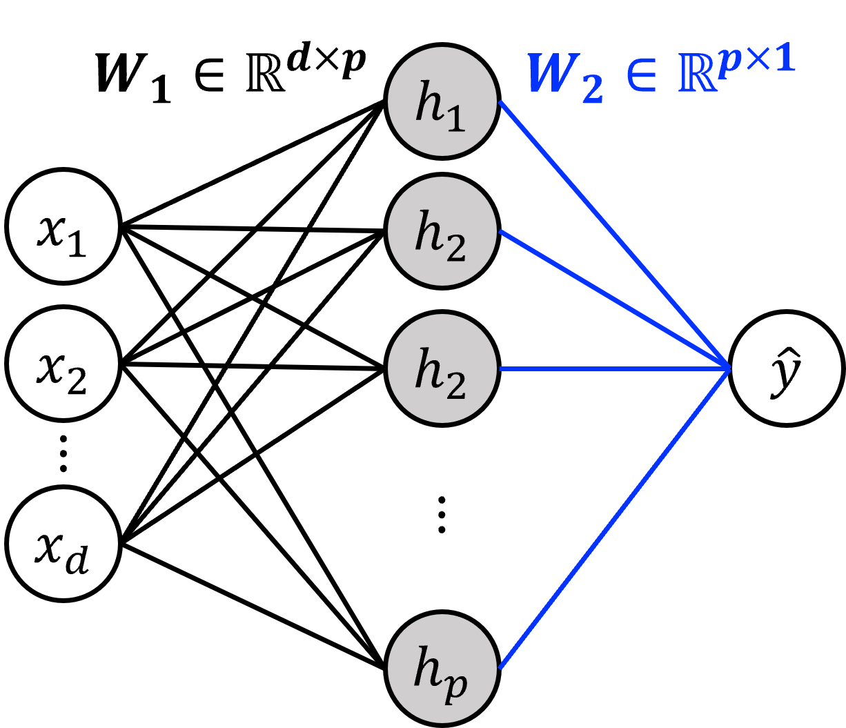
Extreme Learning Machine (ELM) is a feed-forward neural network architecture designed for fast and efficient learning. Introduced to overcome the limitations of traditional learning algorithms, ELM operates with a Single-Layer Fully connected Networks (SLFNs) where the weights between the input and hidden layers are randomly initialized and fixed. This unique feature eliminates the need for iterative tuning of these weights, significantly reducing computational cost. The output weights are determined analytically by minimizing the training error, e.g., least squares, making ELM training extremely fast compared to conventional methods like backpropagation. Its simplicity, efficiency, and capacity for handling large-scale datasets make ELM a powerful tool in various domains, including regression, classification, and feature extraction.
The Universal Approximation Theorem for ELMs establishes that SLFNs with randomly generated hidden parameters can approximate any continuous function on a compact domain, given a sufficient number of neurons [18]. This theoretical foundation has spurred interest in applying ELMs to a variety of tasks, including classification, and regression [19, 20, 21]. More recently, physics-informed learning. ELMs have demonstrated promising results when applied to PINN frameworks, reducing training complexity while maintaining accuracy [22, 23]. This success motivates the application of ELMs to operator learning, particularly for DeepONets.
In this work, we present a novel methodology ELM-DeepONets that combines the strengths of ELM and DeepONets to address the computational challenges in operator learning. Our approach leverages ELM’s efficiency to train DeepONets by solving a least squares problem, bypassing the need for expensive gradient-based optimization. The proposed ELM-DeepONets framework is validated on a diverse set of problems, including nonlinear ODEs and forward-inverse problems for benchmark PDEs. Our experiments demonstrate that the method achieves comparable accuracy to conventional DeepONet training while significantly reducing computational costs. Additionally, we highlight the potential of ELM as a lightweight and scalable alternative for operator learning in scientific computing.
The remainder of this paper is organized as follows. Section 2 briefly introduces important preliminaries to our method. Section 3 details the mathematical framework and implementation of the ELM-based DeepONet. Section 4 presents the results of numerical experiments, showcasing the effectiveness of the proposed method. Finally, Section 5 concludes with a discussion of potential extensions and future research directions.
2 Preliminaries
2.1 Extreme Learning Machines
In this subsection, we briefly outline the ELM with SLFN for the regression problem. Let and be the input data and label, respectively, where is the number of samples and is the input dimension. The network maps to an output using hidden neurons with randomly initialized and fixed weights . The hidden layer output is computed as , where is an activation function applied in an elementwise manner. The output is computed by where . For fixed and , we obtain by least square fit to the label , i.e., where is the Moore-Penrose pseudoinverse of .
2.2 A brief introduction to DeepONets
DeepONet is a recently proposed operator learning framework that is usually trained in a supervised manner. The supervised dataset consists of labeled pairs of functions , where input functions are characterized by -dimensional vector at discrete sensor points and the target function is evaluated at collocation points .
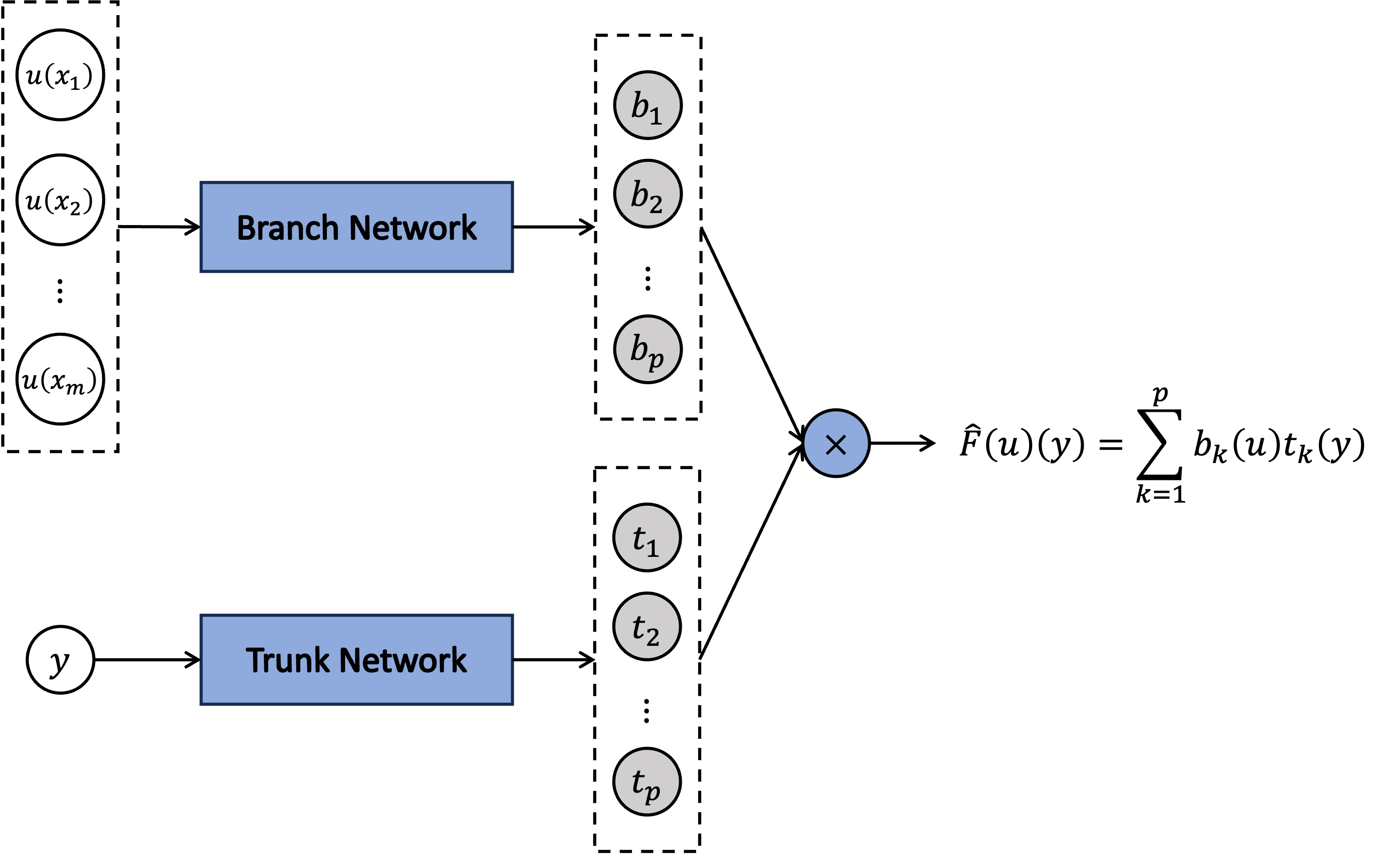
DeepONet comprises two subnetworks, the branch network and the trunk network. The branch network takes the -dimensional vector and generates -dimensional vector . On the other hand, the trunk network takes the collocation point as input to generate another -dimensional vector . Finally, we take the inner product of and to generate the output . Then, two subnetworks are trained to minimize the loss function defined by:
The overall architecture is illustrated in Figure 2.
3 ELM-DeepONets
ELM employs fixed basis functions generated by random parameters and determines the coefficients for their linear combination. Similarly, DeepONet constructs a linear combination of basis functions produced by the trunk network, with the coefficients generated by the branch network. Building on the structural similarity between ELM and DeepONet, we propose a novel framework called ELM-DeepONet.
Recall that the output of DeepONet is expressed as:
where , , are the coefficients generated from the branch network and , , are the basis functions generated from the trunk network. To incorporate the fixed basis functions of ELM into DeepONet, we model using a fully connected neural network with fixed parameters. This modification aligns the trunk network with the ELM philosophy by removing the need to train its parameters. In the standard ELM framework, the coefficients are determined by solving a simple least squares problem. However, in DeepONet, the coefficients are functions of the input , introducing additional complexity that makes it challenging to directly apply the ELM methodology. We address this issue by incorporating an ELM to model the coefficients.
Let
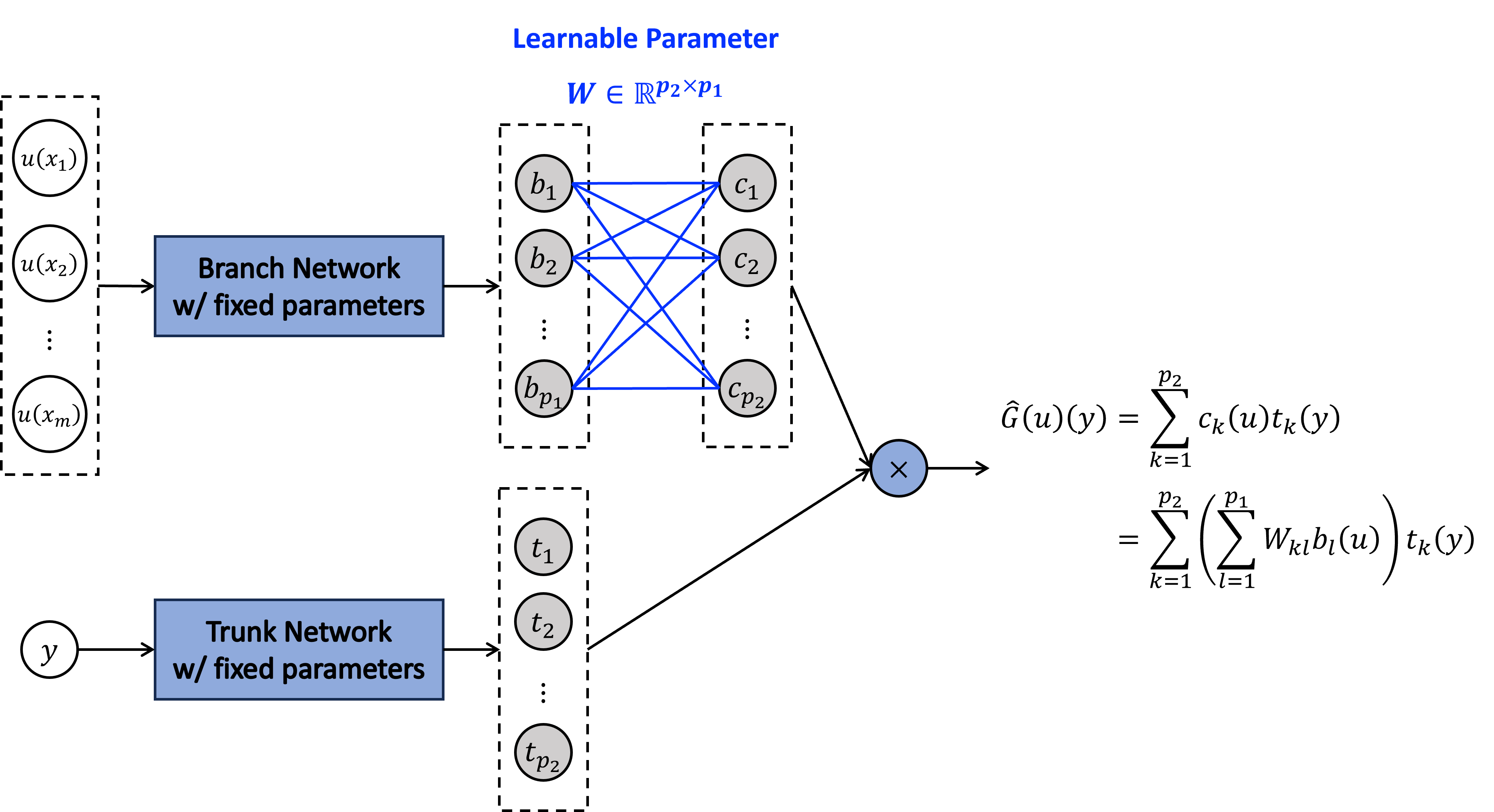
be the ELM-DeepONet output, where , for are the basis functions modeled by the trunk network with fixed parameters, and is a hyperparameter. To compute , we use another fully connected neural network with fixed parameters to generate for , and define as:
where is a learnable parameter. Consequently, the output of ELM-DeepONet can be expressed as:
where and are hyperparameters that will be discussed in detail later. In this novel framework, the only learnable parameter is , while all the parameters in and remain fixed. This design drastically reduces the number of trainable parameters in ELM-DeepONet to which is significantly smaller than that of the vanilla DeepONet. The overall architecture is illustrated in 3.
Let be a supervised dataset for training ELM-DeepONet. Then the objective
can be expressed as:
| (1) |
where denotes the Frobenius norm, and
Here, represents the output of the trunk network, is the learnable parameter, represents the output of the branch network, and is the label.
The objective in Equation (1) can be minimized by using the Moore-Penrose pseudoinverse as:
To solve the equation for , we assume that and are of full rank. By selecting such that , then is of full rank. This allows us to compute the left pseudoinverse of T as:
Similarly, if is chosen such that , then the matrix is of full rank and the right pseudoinverse of can be computed as:
Thus, by setting , and , we obtain the solution of the objective in Equation (1) as:
Consequently, with the proposed ELM-DeepONet, training a DeepONet is reduced to solving a least square problem, which can be efficiently addressed by computing two pseudoinverses.
The proposed ELM-DeepONet architecture offers notable flexibility. For instance, the branch network can utilize a Convolutional Neural Network (CNN) with fixed weights, a modification of the common approach in modern DeepONet architectures [10, 14]. Additionally, since the trunk network is responsible for generating global basis functions, it can be replaced with predefined fixed basis functions, such as or , instead of employing a neural network. These variations are evaluated through numerical experiments to assess their effectiveness and computational efficiency.
4 Numerical Results
We present the numerical results demonstrating the superior performance of the proposed method. All experiments were conducted using a single NVIDIA GeForce RTX 3090 GPU.
4.1 Ordinary Differential Equations
4.1.1 Antiderivative
We consider learning the antiderivative operator:
as studied in [10]. To generate the input functions, we sampled 2000 instances of from a Gaussian Random Field (GRF):
where the covariance kernel is defined by with . Using numerical integration, we created the dataset with , where represents the uniform collocation points. The dataset was split into 1000 training samples and 1000 testing samples.
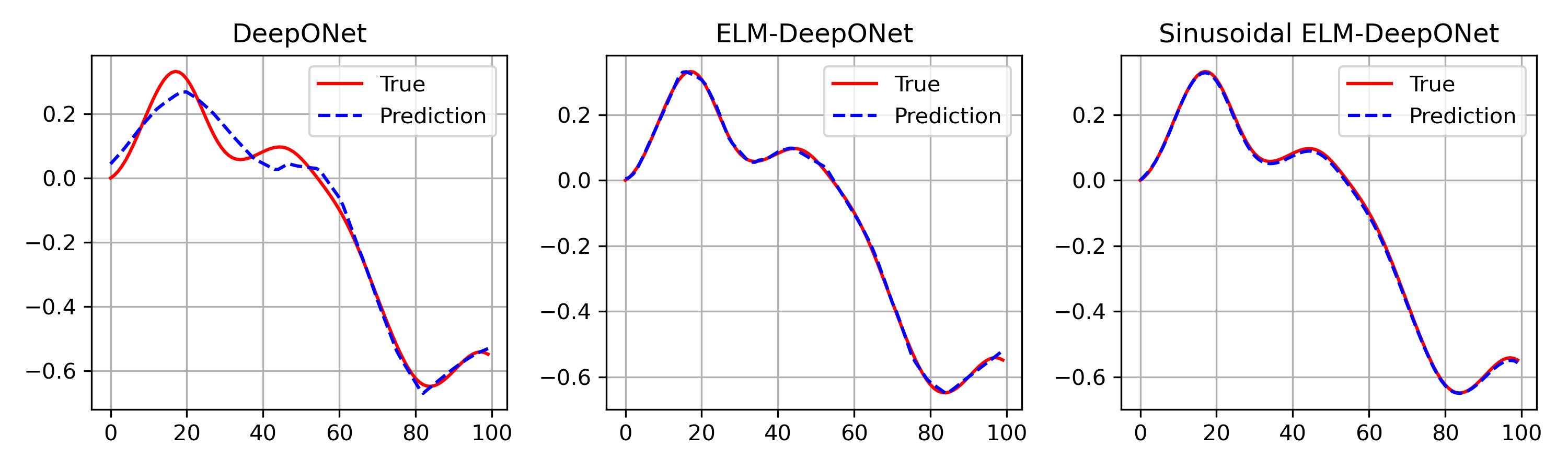
As baseline models, we employed two DeepONets, M1 (Model 1) and M2 (Model 2), each utilizing fully connected neural networks with ReLU activation for both the branch and trunk networks. M1 features branch and trunk networks with architectures 1-64-64-64-1, while M2 employs larger networks with architectures 1-256-256-256-1. We trained the DeepONet by using Adam optimizer with a learning rate 1e-3 for epochs [24]. We fixed the branch network of the ELM-DeepONet with SLFNs with ReLU activation and the trunk network with 3-layer MLP consisting of hidden nodes in each layer. We also tested the sinusoidal basis function (Sinusoidal ELM-DeepONet) rather than the trunk net, such as . In this example, we set and .
The results are summarized in Table 1. As shown, training the ELM-DeepONet requires negligible time compared to the vanilla DeepONets, while the proposed methods achieve significantly lower relative test errors. Figure 4 illustrates the results on a representative test sample.
| Model | # parameters | Training time (s) | Relative error | ||
|---|---|---|---|---|---|
| DeepONet M1 | 23K | 437 | 4.12% | ||
| DeepONet M2 | 290K | 495 | 7.19% | ||
| ELM-DeepONet | 20K | 0.14 | 2.12% | ||
|
20K | 0.11 | 2.45% |
4.1.2 Nonlinear ODE
Next, we focus on learning the solution operator of a nonlinear ODE defined as:
the source function is sampled from the same GRF as described in Section 4.1.1. Using numerical integration, we construct the dataset with , , and . We then compare the relative test errors of the proposed ELM-DeepONet and the Sinusoidal ELM-DeepONet to those of the baseline models M1 and M2. The results are summarized in Table 2.
| Model | # parameters | Training time (s) | Relative error | ||
|---|---|---|---|---|---|
| DeepONet M1 | 23K | 451 | 4.87% | ||
| DeepONet M2 | 290K | 485 | 5.21% | ||
| ELM-DeepONet | 20K | 0.14 | 2.91% | ||
|
20K | 0.11 | 3.39% |
4.2 Sensitivity analysis
The hyperparameters and play a critical role in the performance of ELM-DeepONet. As previously discussed, it is important to set and to satisfy the condition
| (2) |
to ensure that the pseudoinverses and function as left and right inverses, respectively. However, we have observed that, in practice, significantly larger values of and which violate the condition in Equation (2), can still yield satisfactory results. We provide sensitivity analysis for the choice of parameters and through the antiderivative example.
Tables 3 and 4 present the relative errors corresponding to various choices of and . These relative errors were calculated over 10 trials and averaged to ensure statistical reliability. The results reveal several intriguing trends. First, as increases, the relative error consistently grows, reinforcing the empirical validity of the condition . This observation aligns well with theoretical expectations and highlights the importance of carefully constraining for stable performance.
On the other hand, a contrasting pattern emerges for ; the relative error decreases as increases, even when . This behavior deviates from the theoretical condition suggesting that relaxing this constraint might improve performance in practical settings. These findings underline the relationship between the hyperparameters and the model’s performance, offering valuable insights for their optimal selection in ELM-DeepONet.
| 50 | 100 | 500 | 1000 | 5000 | 10000 | |
|---|---|---|---|---|---|---|
| 50 | 15% | 15% | 16% | 17% | 27% | 30% |
| 100 | 8.8% | 8.8% | 9.2% | 11% | 23% | 26% |
| 500 | 3.3% | 3.6% | 5.5% | 8.1% | 22% | 22% |
| 1000 | 2.2% | 2.5% | 4.1% | 7.2% | 22% | 23% |
| 5000 | 1.7% | 1.6% | 2.3% | 7.8% | 20% | 22% |
| 10000 | 1.8% | 1.4% | 3.4% | 7.1% | 22% | 27% |
| 50 | 100 | 500 | 1000 | 5000 | 10000 | |
|---|---|---|---|---|---|---|
| 50 | 15% | 16% | 16% | 14% | 15% | 15% |
| 100 | 7.8% | 7.9% | 7.5% | 8.2% | 7.8% | 8.0% |
| 500 | 5.5% | 5.6% | 5.3% | 5.8% | 5.6% | 5.5% |
| 1000 | 2.7% | 2.6% | 2.7% | 2.7% | 2.6% | 2.7% |
| 5000 | 0.6% | 0.6% | 0.6% | 0.6% | 0.7% | 0.8% |
| 10000 | 0.4% | 0.4% | 0.4% | 0.4% | 0.4% | 0.4% |
4.3 Darcy Flow
Next, we investigate the Darcy Flow, a 2D Partial Differential Equation (PDE) defined as:
where represents the permeability and the source function is given by . The objective is to train the models to learn the solution operator, which maps the permeability field to the corresponding solution
Here is sampled from the GRF to generate diverse input scenarios. We use a uniform mesh in as collocation points. We create the dataset with and .
As a baseline algorithm, we employed two DeepONets with different branch networks. One with a 3-layer MLP with each layer consisting of 128 nodes (DeepONet-MLP), and the other with a Convolutional Neural Network (CNN) with three convolutional layers followed by two fully connected layers (DeepONet-CNN). For the trunk network, we utilized a 3-layer Multilayer Perceptron (MLP), with each layer consisting of 128 nodes. We use ReLU as an activation function for all networks. We trained the network by using Adam optimizer for 10000 epochs with a learning rate 1e-3.
We employed two ELM-DeepONets with MLP branch and CNN branch network, as the DeepONets, with all parameters kept fixed. In the Sinusoidal ELM-DeepONet, the trunk network was replaced with sinusoidal basis functions, specifically: designed to enforce boundary conditions and leverage the advantages of harmonic representations, see Figure 5. We choose the hyperparameters and by using a simple grid search.
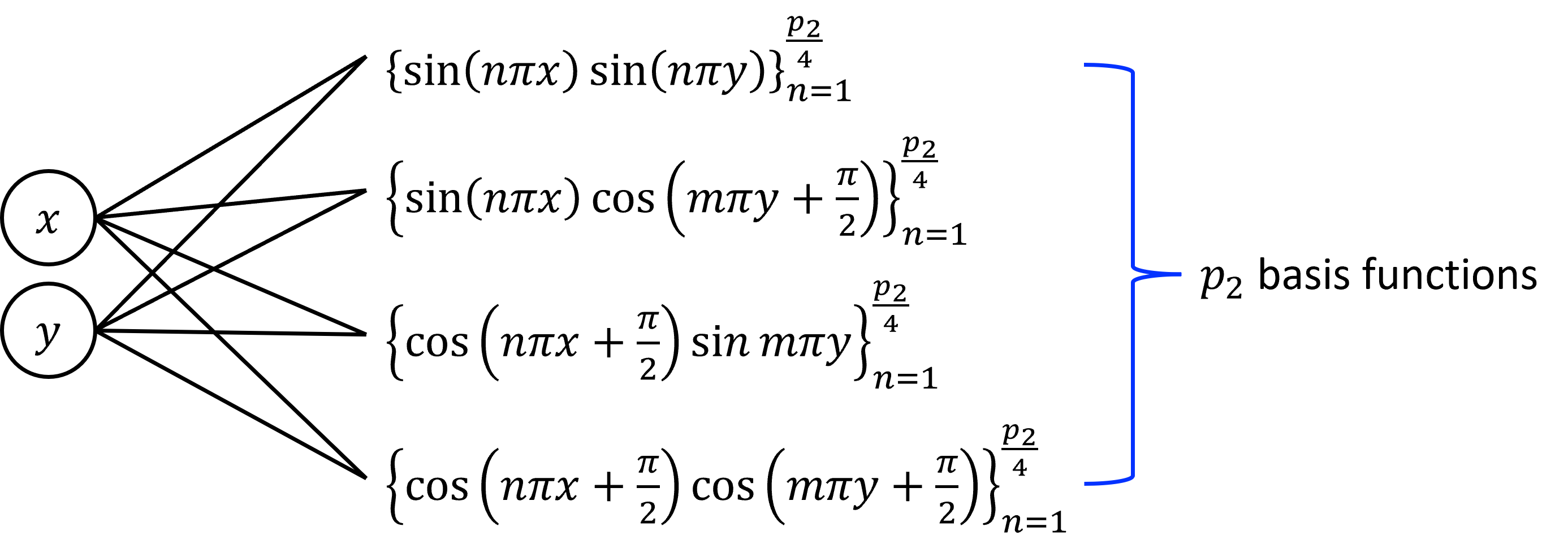
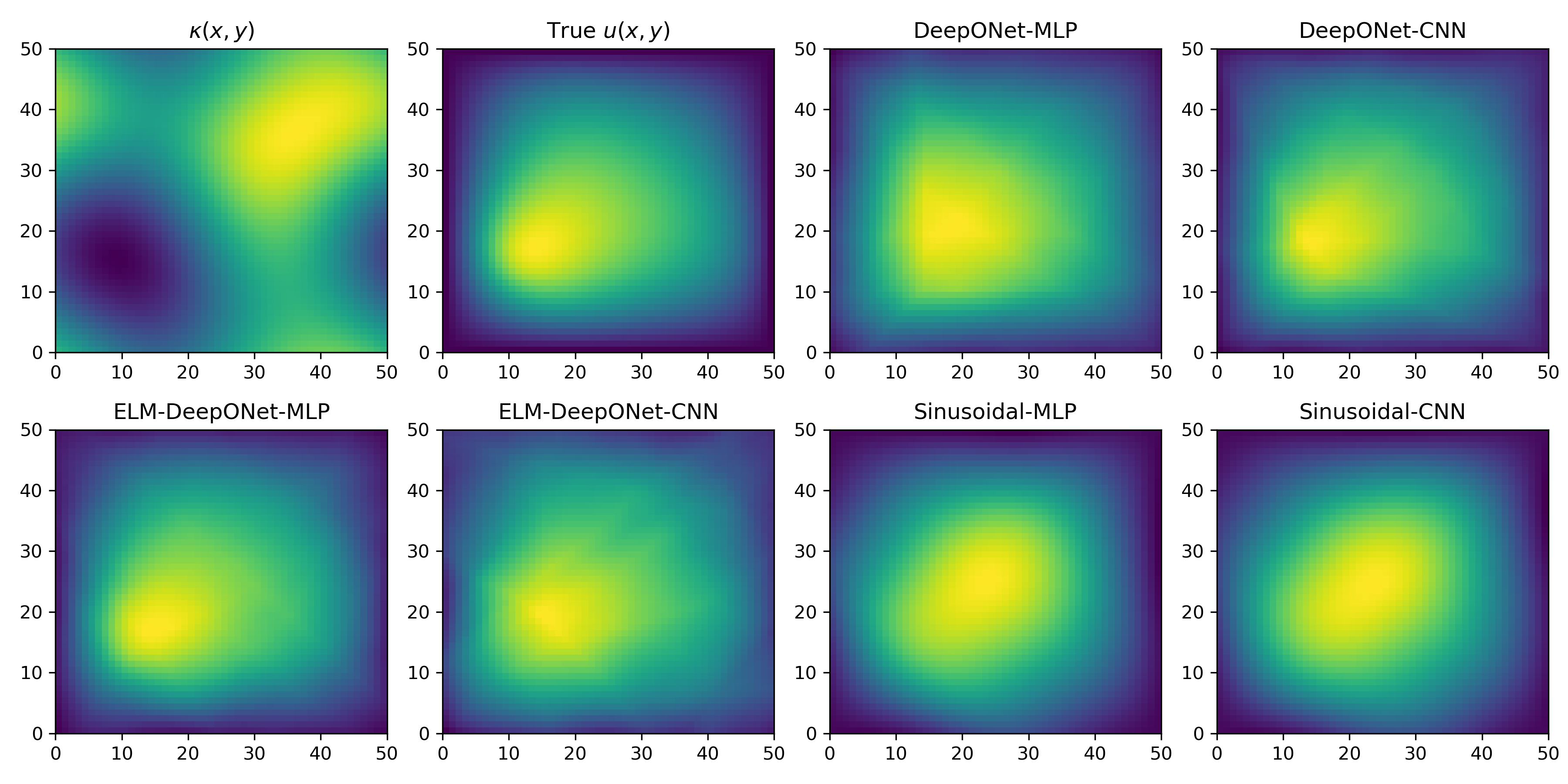
Table 5 showcases the superior performance of ELM-DeepONet compared to the vanilla DeepONet. Among the tested models, the ELM-DeepONet with an MLP branch network outperforms all others, achieving the best results in both relative error and training efficiency. The vanilla DeepONet with a CNN branch network ranks second, demonstrating competitive accuracy but requiring significantly more training time. The notable improvement of ELM-DeepONet with an MLP branch network highlights its ability to combine high accuracy with computational efficiency. Figure 6 visualizes the model predictions for a randomly selected test sample, further illustrating the effectiveness of the proposed approach.
| Model | # parameters |
|
|
|||||
|---|---|---|---|---|---|---|---|---|
| DeepONet | MLP | 181K | 1131 | 11.77% | ||||
| CNN | 68K | 1195 | 6.32% | |||||
| ELM-DeepONet | MLP | 10M | 3.10 | 5.65% | ||||
| CNN | 500K | 3.02 | 6.80% | |||||
|
MLP | 250K | 0.99 | 15.24% | ||||
| CNN | 5M | 3.13 | 15.01% | |||||
4.4 Reaction Diffusion equation: An inverse source problem
We consider an inverse source problem for a parabolic equation, as discussed in both the PINN and operator learning literature [25, 14]. The equation is defined as:
where . The objective is to learn the inverse operator
which maps the boundary observations of to the source term . [25] established that this problem is well-posed.
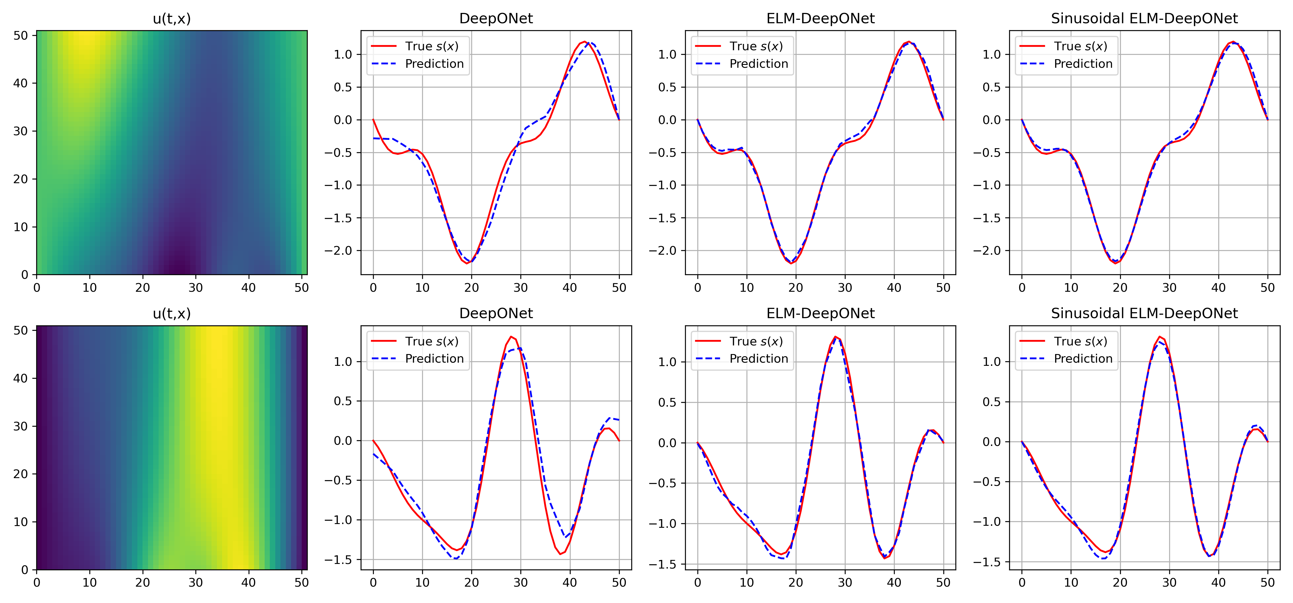
As a baseline algorithm, we employed a vanilla DeepONet with MLP-based branch and trunk networks, each consisting of three layers with 64 nodes per layer. For the ELM-DeepONet, we utilized an SLFN for the branch network and a three-layer MLP for the trunk network. The hyperparameters and were selected using a grid search method. We summarized the result in Table 6, and Figure 7 presents the results on two randomly selected test sample.
| Model | # parameters | Training time (s) | Relative error | ||
|---|---|---|---|---|---|
| DeepONet | 23K | 104 | 5.04% | ||
| ELM-DeepONet | 500K | 0.15 | 2.77% | ||
|
500K | 0.11 | 2.52% |
5 Conclusion
We propose a novel training algorithm, ELM-DeepONet, to enable the efficient training of DeepONet by leveraging the least square formulation and computational efficiency of ELM. Through extensive validation, we have demonstrated that ELM-DeepONet outperforms vanilla DeepONet in both test error and training time. We believe that ELM-DeepONet represents a significant advancement for the operator learning community, addressing the challenge of high computational costs.
We leave several points for future work. First, the choice of and significantly impacts the performance of ELM-DeepONet. Empirically, we observed that larger values of and smaller values of generally lead to better performance. Notably, extremely large , such as , performed well in practice, despite violating our theoretical insight that the pseudoinverse should act as a proper right inverse. A more thorough analysis of this phenomenon would be valuable for further advancing the framework. Second, recent studies have incorporated ELM into Physics-Informed Neural Networks (PINNs). Building on this trend, it is natural to consider extending ELM to Physics-Informed DeepONets as a promising direction for future work.
References
- [1] George Em Karniadakis, Ioannis G Kevrekidis, Lu Lu, Paris Perdikaris, Sifan Wang, and Liu Yang. Physics-informed machine learning. Nature Reviews Physics, 3(6):422–440, 2021.
- [2] Zheyuan Hu, Khemraj Shukla, George Em Karniadakis, and Kenji Kawaguchi. Tackling the curse of dimensionality with physics-informed neural networks. Neural Networks, 176:106369, 2024.
- [3] Justin Sirignano and Konstantinos Spiliopoulos. Dgm: A deep learning algorithm for solving partial differential equations. Journal of computational physics, 375:1339–1364, 2018.
- [4] Min Sue Park, Cheolhyeong Kim, Hwijae Son, and Hyung Ju Hwang. The deep minimizing movement scheme. Journal of Computational Physics, 494:112518, 2023.
- [5] Maziar Raissi, Paris Perdikaris, and George E Karniadakis. Physics-informed neural networks: A deep learning framework for solving forward and inverse problems involving nonlinear partial differential equations. Journal of Computational physics, 378:686–707, 2019.
- [6] Lu Lu, Xuhui Meng, Zhiping Mao, and George Em Karniadakis. Deepxde: A deep learning library for solving differential equations. SIAM review, 63(1):208–228, 2021.
- [7] Shengze Cai, Zhiping Mao, Zhicheng Wang, Minglang Yin, and George Em Karniadakis. Physics-informed neural networks (pinns) for fluid mechanics: A review. Acta Mechanica Sinica, 37(12):1727–1738, 2021.
- [8] Hyeontae Jo, Hwijae Son, Hyung Ju Hwang, and Eun Heui Kim. Deep neural network approach to forward-inverse problems. Networks & Heterogeneous Media, 15(2), 2020.
- [9] Hwijae Son and Minwoo Lee. A pinn approach for identifying governing parameters of noisy thermoacoustic systems. Journal of Fluid Mechanics, 984:A21, 2024.
- [10] Lu Lu, Pengzhan Jin, Guofei Pang, Zhongqiang Zhang, and George Em Karniadakis. Learning nonlinear operators via deeponet based on the universal approximation theorem of operators. Nature machine intelligence, 3(3):218–229, 2021.
- [11] Nikola Kovachki, Zongyi Li, Burigede Liu, Kamyar Azizzadenesheli, Kaushik Bhattacharya, Andrew Stuart, and Anima Anandkumar. Neural operator: Learning maps between function spaces with applications to pdes. Journal of Machine Learning Research, 24(89):1–97, 2023.
- [12] Zongyi Li, Nikola Kovachki, Kamyar Azizzadenesheli, Burigede Liu, Kaushik Bhattacharya, Andrew Stuart, and Anima Anandkumar. Fourier neural operator for parametric partial differential equations. arXiv preprint arXiv:2010.08895, 2020.
- [13] Sifan Wang, Hanwen Wang, and Paris Perdikaris. Learning the solution operator of parametric partial differential equations with physics-informed deeponets. Science advances, 7(40):eabi8605, 2021.
- [14] Sung Woong Cho and Hwijae Son. Physics-informed deep inverse operator networks for solving pde inverse problems. arXiv preprint arXiv:2412.03161, 2024.
- [15] Michael Prasthofer, Tim De Ryck, and Siddhartha Mishra. Variable-input deep operator networks. arXiv preprint arXiv:2205.11404, 2022.
- [16] Jae Yong Lee, Seungchan Ko, and Youngjoon Hong. Finite element operator network for solving parametric pdes. arXiv preprint arXiv:2308.04690, 2023.
- [17] Junho Choi, Namjung Kim, and Youngjoon Hong. Unsupervised legendre–galerkin neural network for solving partial differential equations. IEEE Access, 11:23433–23446, 2023.
- [18] Guang-Bin Huang, Lei Chen, and Chee-Kheong Siew. Universal approximation using incremental constructive feedforward networks with random hidden nodes. IEEE transactions on neural networks, 17(4):879–892, 2006.
- [19] Shifei Ding, Xinzheng Xu, and Ru Nie. Extreme learning machine and its applications. Neural Computing and Applications, 25:549–556, 2014.
- [20] Gao Huang, Guang-Bin Huang, Shiji Song, and Keyou You. Trends in extreme learning machines: A review. Neural Networks, 61:32–48, 2015.
- [21] Jian Wang, Siyuan Lu, Shui-Hua Wang, and Yu-Dong Zhang. A review on extreme learning machine. Multimedia Tools and Applications, 81(29):41611–41660, 2022.
- [22] Vikas Dwivedi and Balaji Srinivasan. Physics informed extreme learning machine (pielm)–a rapid method for the numerical solution of partial differential equations. Neurocomputing, 391:96–118, 2020.
- [23] Xi’an Li, Zhe Ding, Jinran Wu, Xin Taia, Liang Liua, and You-Gan Wang. Augmented physics informed extreme learning machine to solve the biharmonic equations via fourier expansions.
- [24] Diederik P Kingma. Adam: A method for stochastic optimization. arXiv preprint arXiv:1412.6980, 2014.
- [25] Mengmeng Zhang, Qianxiao Li, and Jijun Liu. On stability and regularization for data-driven solution of parabolic inverse source problems. Journal of Computational Physics, 474:111769, 2023.