Non-linear Partition of Unity method
Abstract
This paper introduces the Non-linear Partition of Unity Method, a novel technique integrating Radial Basis Function interpolation and Weighted Essentially Non-Oscillatory algorithms. It addresses challenges in high-accuracy approximations, particularly near discontinuities, by adapting weights dynamically. The method is rooted in the Partition of Unity framework, enabling efficient decomposition of large datasets into subproblems while maintaining accuracy. Smoothness indicators and compactly supported functions ensure precision in regions with discontinuities. Error bounds are calculated and validate its effectiveness, showing improved interpolation in discontinuous and smooth regions. Some numerical experiments are performed to check the theoretical results.
keywords:
WENO , high accuracy approximation , improved adaption to discontinuities , RBF , 41A05 , 41A10 , 65D05 , 65M06 , 65N061 Introduction
Kernel-based methods are useful and powerful tools employed in several fields of science as computer aided design, numerical resolution of partial differential equations, image processing or others. These schemes are satisfactory used in interpolation, regression and machine learning due to their easy and quick implementation and their simple generalization for any dimension.
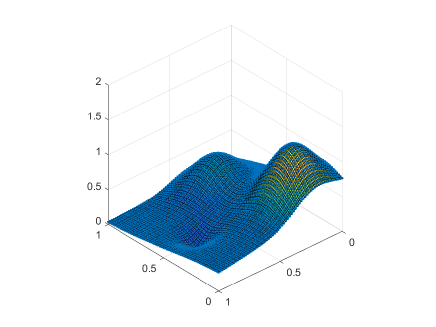
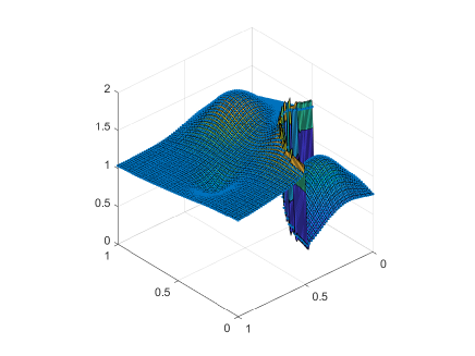
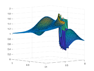
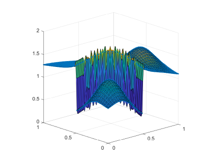
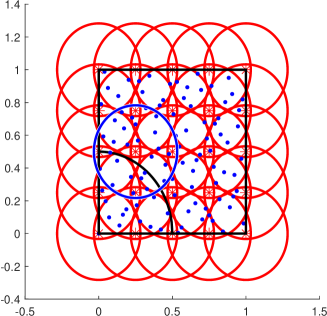
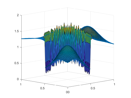
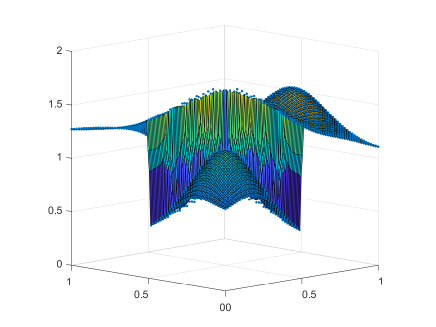
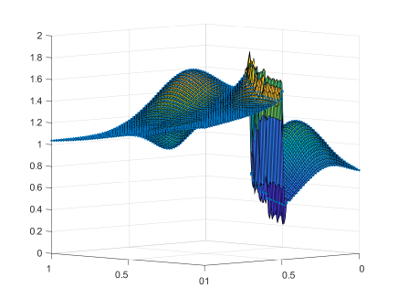
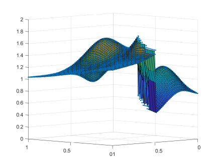
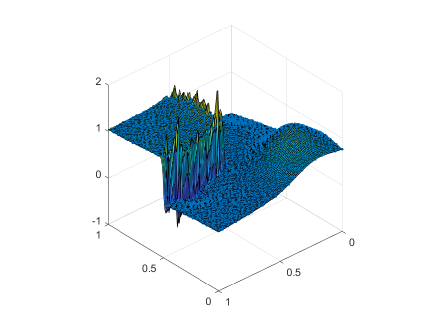
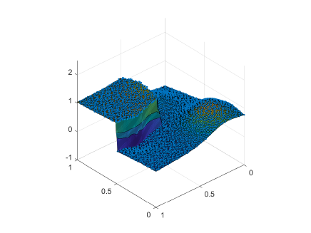
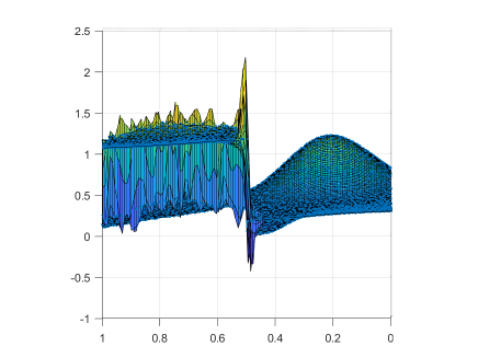
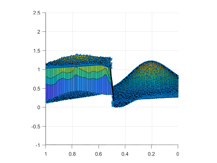
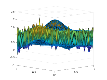
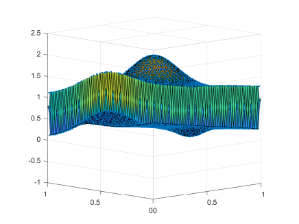
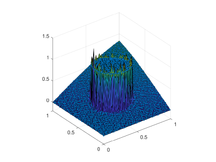
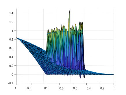
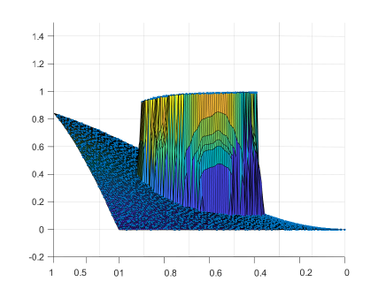
The problem consists in finding a good approximation to an unknown function, , from some data values given a set of arbitrarily distributed points on an open and bounded domain , . Radial basis function method (RBF) consists on developing the function as a linear combination of a basis of radial functions centered in the data points . There exists a vast literature about it (see, e.g. [5, 9, 19]), however the efficiency of the method can be improved in different ways. One approximation, called partition of unity method (PUM or PU method) (see e.g. [5, 6, 7, 9, 19]) involves partitioning the entire domain into multiple smaller subdomains and applying the RBF method to each of them. Ultimately, a convex combination of these interpolants yields the final approximation. Satisfactory results are obtained when these methods are employed to data originating from continuous function, see for example, the approximation presented in Fig. 1 (a) where we approximate the Franke’s function:
| (1) |
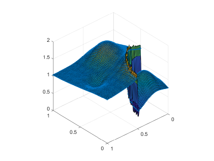
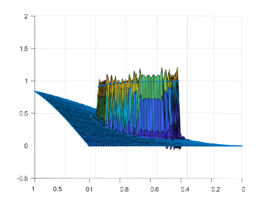
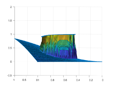
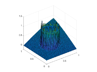
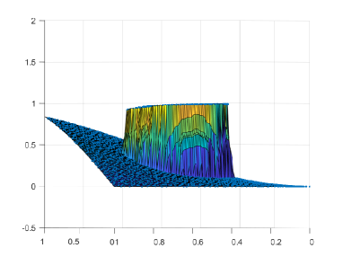
using the PU method with data points located at . However, these methods yield inadequate results when the data originates from functions with discontinuities. See for example Figs. 1 (b), (c) and (d), where we present the result obtained when applying the PUM to the piecewise smooth function:
| (2) |
It is clear that we can observe some oscillations close to the discontinuities. In order to avoid these non-desirable effects, non-linear methods can be applied when approximating this kind of data. In particular, we reformulate the PUM using Weighted Essentially Non-Oscillatory (WENO) techniques, designed by Liu et al in [15] and extensively developed by Shu (see [17]). The basic idea is to modify the weights of the partition of unity by replacing them with non-linear ones that depend on the data . This way, when a discontinuity crosses a subdomain, the approximation is not considered. It is not difficult to prove that the order of accuracy is conserved in all the domain, except in a band close to the discontinuity.
|
|
| (a) | (b) |
|
|
| (c) | (d) |
The paper is divided in the following sections: In Section 2, we start by reviewing the RBF interpolation and showing some theorems where the error bounds are estimated, Sec. 3 is devoted to introduce the PUM and to prove the theoretical results related to the order of accuracy. Afterwards, in Section 4, we review WENO method from the PUM perspective, identifying each component of WENO with its corresponding component in PUM. The non-linear method is presented in Sec. 5 where we explain its theoretical properties and its implementation. Some numerical results are performed in Sec. 6 and some conclusions and future work are outlined in the last section.
2 Radial Basis Function Interpolation
There is extensive literature on the RBF interpolation method (see e.g. [5, 9, 19]), we will principally employ the notation presented in [8, 9]. We consider a set of scattered data in a bounded domain , with an associated set of data values which are the evaluations of certain unknown function at the nodes . The scattered data interpolation problem is the following: to find an operator, , such that:
Ideally, we aim to minimize the distance between and in a specified norm. First, we define a radial function when there exists a univariate function such that
with the Euclidian norm in Now, we denote as , and use a radial basis function expansion to formulate the problem:
| (3) |
being the coefficients that solve the interpolation system with
It is clear that is symmetric and some conditions over has to be imposed to get a matrix definite positive and, therefore, a unique solution of the system. Next definition is useful for this purpose (see [9]).
Definition 1 ([9])
A real continuous function is called positive definite on if
| (4) |
for any pairwise different points and . It is strictly positive definite on if the form (4) is zero only for .
In the literature we can find many examples of functions which produce strictly positive definite functions, such as Gaussian function , that is also . Another example are Wendland functions, defined as
| (5) |
based on the cutoff function
which are , and respectively. Matérn functions are another example, that are defined as
| (6) |
satisfying that , . Other classes of functions, such as generalized inverse multiquadrics or Poisson radial functions, also produce strictly positive definite functions, see [9] for more details.
The first characteristic of this interpolant, Eq. (3), is the smoothness, as it is a linear combination of smooth functions, . Consequently, the continuity of the operator only depends on the continuity of the function .
Secondly, the error estimates and the order of accuracy for the interpolation process have been studied extensively (see [5, 9, 19] and the references cited therein for further details). To introduce the results, we need to present three relevant concepts: First of all, we define the fill distance, which measures the extent to which the data in the set adequately cover the domain , as
Following this, we refer to the space (see [7, 9])
and finally, we state that a region satisfies an interior cone condition, [9, 19], if there exists an angle and a radius such that for every there exists a unit vector such that the cone
The following lemma presented by Wendland in [19] indicates that a ball always satisfies an interior cone condition. This result will be relevant in our numerical experiments when we construct a particular partition of unity method.
Lemma 2.1
Every ball with radius satisfies an interior cone condition with radius and angle .
With these three elements: the fill distance, the space and the interior cone condition, we review the following result.
Theorem 2.2
In this work, we focus on studying the differences between the function and the interpolator. Error estimates for the derivatives are proved in [9, 19]. To conclude this review section, we introduce the following results for Matérn function, Eq. (6), as they will be used in the numerical experiments. For this purpose, we need to define the Sobolev spaces introduced in [9] as
Proposition 2.3
Next subsection is devoted to introduce the partition of unity method for radial basis functions, which is a well-known approximation method that is satisfactorily used when the number of data points is very large.
3 Partition of Unity Approximation
The partition of unity method (PUM) is proposed to facilitate efficient computation using meshfree approximation methods. The approach is straightforward: it involves decomposing the large problem into smaller subproblems while preserving the order of accuracy. Accordingly, using the same notation as above, let represent our open and bounded domain, which we partition into subdomains such that [7, 18]:
-
•
The domain is contained in the union of the subdomains, i.e.
-
•
For every the number of subdomains with is bounded by a global constant .
-
•
There exists a constant and an angle such that every patch satisfies an interior cone condition with angle and radius .
-
•
The local fill distance with are uniformly bounded by the global fill distance .
This is called a regular covering for , [19]. For this covering, we choose a partition of unity, i.e. a family of compactly supported, non-negative, continuous functions, with
and define the global interpolator as:
| (7) |
where is a local RBF interpolant on each sudomain .
In [9] some technical conditions over the partition of unity functions are imposed to establish error bounds. We assume that the partition of unity functions is -stable. This is, each and for every multi-index with the following inequality is satisfied:
where is some positive constant and is the diameter of , i.e. . With these restrictions over the covering and the partition of unity function, we show the following result, [9].
Theorem 3.1
Suppose is open and bounded, and let . Let be strictly positive definite. Let be a regular covering for and let be -stable for . Then the error between and its partition of unity interpolant, Eq. (7), can be bounded by
for all .
It is clear that the order of accuracy does not vary using PUM or RBF method, as we can see in the theorems 2.2 and 3.1. A simple way, suggested in [7, 9], to construct PUM is to consider Shepard’s approximation, i.e.
| (8) |
where are compactly supported, with their support contained in , and can be chosen, for example, as Wendland functions, Eq. (5).
4 Reviewing Weighted Essentially Non-Oscillatory algorithm as a PUM
The WENO scheme has gained widespread recognition as an effective method for approximating data values, especially in contexts where discontinuities are prevalent (see e.g. [17]). Initially introduced for approximatig the solution of hyperbolic partial differential equations, the WENO approach is structured to achieve high-order accuracy while mitigating the unwanted oscillations that typically occur near discontinuities [12]. This is accomplished through the adaptive assignment of weights that prioritize smoother portions of the data and diminish the contribution of stencils that intersect discontinuities.
In what follows, we review the WENO- method in the point-values context (see [1, 2]) relating each of its component to those corresponding to the PUM. The analogy is done for the algorithms in one variable, but it can be generalized to several variables [16]. In this case, let be a uniform partition of the interval in subintervals, and let be the point-values discretization of an unknown function at the nodes , to interpolate at . WENO- algorithm uses the stencil , that is composed of nodes, we denote it by . We can divide the stencil in substencils of nodes, , and prove that there exist , , [16], called optimal weights, such that:
with and . This is a PU-like method, with and the Lagrange interpolatory polynomial using the nodes . Now, the WENO method consists in replacing by non-linear weights , such that
| (9) |
where the non-linear weights are defined as:
| (10) |
being smoothness indicators which indicates if a discontinuity crosses , is a small positive parameter to avoid division by zero, and is typically a constant to enhance accuracy in smooth regions. The idea is to make a non-linear version of the interpolator , Eq. (7), (NL-PUM) using the ideas of WENO method. The key is to define an adequate smoothness indicator for our framework.
5 Non-linear partition of unity method
As we mentioned in the previous section, Sec. 4, we construct a non-linear PUM starting with the interpolator , Eq. (7):
replacing the weight functions described in Eq. (8) by non-linear ones in the same way as in Eq. (10), i.e.
where is a positive constant, and are compactly supported functions with support on . Note that the new functions are compactly supported and, if we choose as Wendland functions, then are Wendland functions too. The constant is set to avoid non-zero denominators. The parameter is relevant to correctly detect the discontinuities and we choose . Finally, , are the smoothness indicators. To construct them, we consider
with , and the linear least square problem
where is the set of polynomials of degree less than or equal to one, and define
| (11) |
then satisfies the conditions:
-
•
The order of the smoothness indicator that are free of discontinuities is , i.e.
-
•
When a discontinuity crosses then:
Therefore, the new non-linear operator will be:
| (12) |
The key to this new method is that it gives more weight to the data placed in smooth regions of the data, neglecting data located near the discontinuity, as this data is multiplied by a weight of order . In the next subsection we will analyze the properties of the interpolator.
5.1 Properties of the new NL-PUM
From the new interpolator, Eq. (12) is defined as PUM multiplying the compactly supported functions by constants (that are dependent on the data ). The smoothness of the new operator is similar to PUM, int he sense that its smoothness is solely determined by the smoothness of the functions and .
Secondly, we determine the order of accuracy when we apply to data that comes from a function which is piecewise continuous throughout its subdomains but not continuous, i.e. we suppose an open and bounded domain and consider a curve , and the sets
that is to say that is divided into two subsets, . Let us assume that our data originates from a function of the type:
with , , but
then our scattered data are divided in two . We select our partition as in Section 3 and define patches that are contaminated by a discontinuity as follows.
Definition 2 (Contaminated patches)
Using the notation presented above, is a contaminated patch if there exist and .
We determine if a subset is a contaminated patch if . Also, the points close to the discontinuity will be marked using the following definition.
Definition 3 (Discontinuity points)
Using the notation above presented, let be a point of the domain, be a fixed threshold and
then is a discontinuity point if
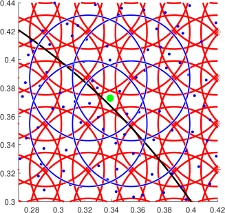
This definition means that a point is a discontinuity point only if all the patches used to interpolate at that point are contaminated, Def. 2. Last definition, Def. 3, is quite relevant to design the new algorithm. This is due to the fact that, at the discontinuity points, the strategy to interpolate has to be changed due to the oscillations produced by the RBF method close to the discontinuity curve. Hence, the most problematic case is the one in which all the patches containing the point where the interpolation is desired, , are contaminated, except for one whose weight, , is close to zero. For this reason, we impose the threshold condition in the previous definition, Def. 3. In Fig. 2 we can see a picture with the representation of the two previous concepts, Defs. 2 and 3. We represent the data points using blue dots, the patch boundaries with red circles, the discontinuity curve and the domain boundary with black lines, and the patch centers with red stars. In the figure on the left, the contaminated patch is indicated with a blue circle. In the figure on the right, the point at which the function is to be approximated is marked in green, while the patches used for interpolation are highlighted in blue. It can be observed that all the patches are contaminated, indicating that the green point is a discontinuity point.
 |
 |
With these definitions, the following result is straightforward based on Th. 3.1, where an error bound is deduced dependent on the smoothness of the function and its native space .
Theorem 5.1
Suppose is open and bounded, and let . Let be strictly positive definite. Let be a regular covering for and let be -stable for . Then, if , it is not a discontinuity point, Def. (3), and , the error between and its non-linear partition of unity interpolant, Eq. (12), with can be bounded by
Analogously, if and it is not a discontinuity point.
In other words, if and there exists, at least, a patch free of discontinuities, then the order of accuracy is conserved. Consequently, the discontinuity points have to be treated in a special manner. Also, if we suppose (without loss of generality) that
we can not ensure that if is a discontinuity point then
For this reason, in order to avoid some oscillations of the interpolator close to the discontinuities, we modify our algorithm and explain it in the next subsection.
5.2 On the implementation of the method. Avoiding oscillations close to the discontinuities
We compute our method using the implementation explained by Cavoretto et al. in [8], based on the partitioning data procedures proposed in [6]. Let be a sample where we want to approximate the function , we start with the covering of the domain , consider some centers , fix a radius and construct the subdomains where is a ball of center and radius . It is important to remark, as noted in [8, 9], that if a nearby node distribution is chosen, is an adequate number of PU subdomains if
then, the radius has to satisfy the condition, [8]:
| (13) |
At this point, we estimate the smoothness indicators , Eq. (11) and mark the contaminated patches, Def. 2. The interpolation data located in each subdomain are found using the partitioning data structures explained in [8]. After this, we estimate the non-linear weights in each point using the smoothness indicators calculated, and label the discontinuity points, we called them . We apply the classical Shepard’s method only for these points, with the same compactly supported function used in PUM. In summary, we describe the algorithm in two passes:
-
1.
We use the software designed in [8] and mark the discontinuity points, .
-
2.
We apply the Shepard’s method to these discontinuity points.
Due to the partitioning data structures introduced in [8], which allow us to organize data very efficiently across different subdomains, the modifications inserted to make the algorithm non-linear are not too costly in terms of computational efficiency.
6 Numerical experiments
In this section, we perform some tests in order to check two principal properties of the new non-linear algorithm, NLPUM, in comparison with the classical one, PUM. We will conduct the experiments using a uniform grid and Halton’s points as data. Firstly, in Subsection 6.1, we employ our method with a continuous function, in particular with Franke’s function, Eq. (1), to verify the order of accuracy. Next subsection is devoted to analyze the elimination of the non-desired oscillations close to the discontinuities, we come back to the example presented in the introduction, Sec. 1, and show the powerful capabilities of the new algorithm for this type of functions. We take the same parameters as [8] in all the experiments, i.e., the number of patches in one direction is and the radius .
6.1 Order of accuracy
We begin by analyzing the order of accuracy using the widely recognized Franke’s function, Eq. (1), using as data points a regular grid defined by , and a set of Halton’s scattered data points, [11]. We denote the fill distance by , and the errors by , where is a regular grid in . We define the maximum discrete norms and their respective convergence rates as follows:
In the first example, we choose Matèrn function, for the RBF problems and the Wendland function , for the partition of unity. We present the results in Table (1), and it is clear that they are very similar for both the linear and non-linear methods. The expected theoretical order of accuracy, Prop. (2.3), is improved for the two algorithms in this example. With respect to the errors, the NLPUM yields slightly better results when the data is placed on an uniform grid.
| Grid points | Halton’s points | ||||||||||
|---|---|---|---|---|---|---|---|---|---|---|---|
| PUM | NLPUM | PUM | NLPUM | ||||||||
| 7.5944e-03 | - | 2.8436e-01 | - | 1.4157e-02 | - | 2.6937e-02 | - | ||||
| 1.6541e-03 | 2.1989 | 8.6890e-02 | 1.7105 | 2.6921e-03 | 2.1831 | 2.9567e-03 | 2.9058 | ||||
| 3.7494e-04 | 2.1413 | 8.8016e-05 | 9.9472 | 9.1058e-04 | 2.3481 | 6.6469e-04 | 3.2331 | ||||
| 1.1278e-04 | 1.7332 | 2.6376e-05 | 1.7385 | 2.0617e-04 | 1.9743 | 3.0466e-04 | 1.0369 | ||||
| 2.8906e-05 | 1.9640 | 7.0429e-06 | 1.9050 | 6.0296e-05 | 1.4750 | 7.9830e-05 | 1.6068 | ||||
| PUM | NLPUM | PUM | NLPUM | ||||||||
| 1.3800e-03 | - | 9.6360e-02 | - | 6.8732e-03 | - | 9.6360e-02 | - | ||||
| 2.2904e-04 | 2.5910 | 4.7798e-03 | 4.3334 | 3.3489e-04 | 2.2581 | 4.7798e-03 | 3.9740 | ||||
| 5.8939e-05 | 1.9583 | 1.5566e-05 | 8.2624 | 3.8497e-05 | 2.7589 | 1.5566e-05 | 4.6860 | ||||
| 1.8977e-05 | 1.6350 | 1.9141e-06 | 3.0236 | 5.9659e-06 | 1.8766 | 1.9141e-06 | 2.4782 | ||||
| 4.0380e-06 | 2.2325 | 2.5281e-07 | 2.9206 | 7.4670e-07 | 1.7219 | 2.5281e-07 | 2.4933 | ||||
To finish this subsection, we repeat the experiment using the functions for the RBF method and for the partition of unity. The results are shown in Table 2. Again, we can see that the errors and orders of accuracy are very similar.
| Grid points | Halton’s points | ||||||||||
|---|---|---|---|---|---|---|---|---|---|---|---|
| PUM | NLPUM | PUM | NLPUM | ||||||||
| 6.4397e-03 | - | 2.9103e-01 | - | 8.1704e-03 | - | 8.7701e-03 | - | ||||
| 7.6400e-04 | 3.0754 | 9.0838e-02 | 1.6798 | 8.9459e-04 | 2.9091 | 1.1375e-03 | 2.6863 | ||||
| 7.3358e-05 | 3.3805 | 2.0297e-05 | 12.1278 | 3.0378e-04 | 2.3397 | 1.6615e-04 | 4.1672 | ||||
| 9.0336e-06 | 3.0216 | 1.6754e-06 | 3.5986 | 2.2676e-05 | 3.4490 | 4.5792e-05 | 1.7129 | ||||
| 1.5305e-06 | 2.5613 | 2.5780e-07 | 2.7002 | 2.3915e-06 | 2.6987 | 1.0517e-05 | 1.7650 | ||||
| PUM | NLPUM | PUM | NLPUM | ||||||||
| 1.0412e-03 | - | 1.0168e-01 | - | 9.6168e-04 | - | 2.6447e-03 | - | ||||
| 1.0970e-04 | 3.2465 | 4.7209e-03 | 4.4289 | 1.0395e-04 | 2.9260 | 1.2230e-04 | 4.0427 | ||||
| 1.2027e-05 | 3.1893 | 2.7164e-06 | 10.7631 | 1.3923e-05 | 4.3550 | 6.5149e-06 | 6.3522 | ||||
| 1.8291e-06 | 2.7170 | 1.5998e-07 | 4.0858 | 1.7160e-06 | 2.7826 | 6.6212e-07 | 3.0389 | ||||
| 1.9361e-07 | 3.2400 | 1.0651e-08 | 3.9088 | 2.0360e-07 | 2.5573 | 5.6579e-08 | 2.9512 | ||||
6.2 Avoiding discontinuities
In this subsection, we conduct a series of experiments to analyze the behavior of the new interpolator near discontinuities. In all the experiments the initial number of data points is .
We begin with a set of experiments in which the original domain is divided into two subdomains. We assume that the data originates from Franke’s function , as defined in Eq. (1), in one subdomain, and from in the other, i.e., we define the functions:
where , , . In this series of experiments we employ as function for RBF problems and for the partition of unity.
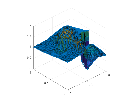
Let us start with the example presented in the introduction, Sec. 1, where the discontinuity curve is the following
In this case, we plot in Fig. 3 the result of the experiment with equidistant points in the square . It is clear, Fig. 3 right column, that NLPUM presents an adequate behaviour close to the discontinuities whereas the PUM produces some oscillations. When the figure is rotated (Fig. 3 rows 2 and 3), the differences become even more evident.
| PUM | NL-PUM |
|---|---|
|
|
|
|
|
|
We also discuss the results when the discontinuities are horizontal, vertical and diagonal lines. For this, we computed a first example with:
and a second with
We illustrate the interpolators for the function in Fig. 4 and for in Fig. 5. In these cases we take initial Halton’s points and we approximate at final points. Again, we can see that the new method avoids the oscillations.
| PUM | NL-PUM |
|---|---|
|
|
|
|
| PUM | NL-PUM |
|---|---|
|
|
To finalize this subsection, we apply the algorithms to the same function employed in [3],
| (14) |
We plot the result using for RBF problems and for partition of unity in Fig. 6 using Halton’s points. Finally, we illustrate the interpolants employing and in Fig. 7 using in the two first rows gridded data points and the two last rows Halton’s point. The interpolators in both cases are very similar. Again, we can see that the new method improves the behaviour close to the discontinuities.
| PUM | NL-PUM |
|---|---|
|

|
|
|
Furthermore, in Fig. 7 we perform the experiment for Halton and grided data points. The oscillations obtained when the classical PUM is applied are highly significant in contrast to the result obtained when the NLPUM is employed.
| PUM | NL-PUM |
|---|---|

|

|
|
|
|

|

|
|
7 Conclusions and future work
The Non-linear Partition of Unity Method (NL-PUM) presented in this study marks a substantial improvement in interpolation techniques, offering a robust solution to challenges posed by discontinuities in datasets. It is founded on integrating Radial Basis Function (RBF) interpolation with Weighted Essentially Non-Oscillatory (WENO) and improves the result obtained by traditional PUM algorithms if the data contains discontinuities. By dynamically adjusting weights through smoothness indicators, NL-PUM selectively conserves the accuracy in smooth regions while minimizing oscillations near discontinuities. These compactly supported, dynamically weighted functions allow for efficient computation without compromising precision.
Numerical experiments confirmed that the NL-PUM maintains the order of accuracy expected from traditional methods in continuous domains while exhibiting superior performance in discontinuous settings. This is achieved by identifying and treating “contaminated patches” near discontinuities, effectively eliminating oscillations that commonly arise in such scenarios. The method’s ability to consistently produce reliable results, regardless of the orientation or complexity of discontinuities, serves to emphasize its robustness. Additionally, the computational efficiency achieved through advanced data partitioning techniques ensures scalability and applicability across various domains.
While the NL-PUM demonstrates promising capabilities, it also presents certain limitations, such as its reliance on well-tuned parameters. These factors highlight the need for further research to optimize and simplify the method. Future work could focus on automating parameter selection, extending the framework to higher-dimensional problems, and exploring its application in practical contexts such as image processing and fluid dynamics. The potential to integrate NL-PUM with other techniques or enhance its adaptability paves a way for further investigation in the near future.
References
- [1] S. Amat, J. Ruiz, C.W. Shu, D. F. Yáñez, (2020): “A new WENO- Algorithm with progressive order of accuracy close to discontinuities”, SIAM J. Numer. Anal., 58(6), 3448-3474.
- [2] F. Aràndiga, A. M. Belda, P. Mulet, (2010): “Point-Value WENO Multiresolution Applications to Stable Image Compression”, J. Sci. Comput., 43(2), 158–182
- [3] S. Amat, D. Levin, J. Ruiz-Álvarez, D. F. Yáñez, (2024): “Non-linear WENO B-spline based approximation method”, Numer. Algor., 100 (10).
- [4] F. Aràndiga and R. Donat, (2000) “Nonlinear multiscale decompositions: The approach of Ami Harten”, Numer. Algorithms, 23:175–216, 2000.
- [5] M. D. Buhmann, (2003). “Radial Basis Functions: Theory and Implementations”, Cambridge University Press.
- [6] R. Cavoretto, A. De Rossi, (2015): “A trivariate interpolation algorithm using a cube-partition searching procedure”, SIAM J. Sci. Comput. 37, A1891–A1908.
- [7] R. Cavoretto, A. De Rossi,E. Perracchione, (2016): “Efficient computation of partition of unity interpolants through a block-based searching technique”, Comput. Math. Appl. 71, 2568–2584.
- [8] R. Cavoretto, A. De Rossi, E. Perracchione, S. Lancellotti, (2022): “Software Implementation of the Partition of Unity Method ”, Dolomites Research Notes on Approximation 15(2), 35–46.
- [9] G. E. Fasshauer: Meshfree Approximation Methods with Matlab, World Scientific Publishing, Singapore, 2007.
- [10] D. Gottlieb, C-W. Shu, (1997): “On the Gibbs phenomenon and its resolution”, SIAM Rev., 39 (4), 644-668.
- [11] J.H. Halton, (1960): “On the efficiency of certain quasi-random sequences of points in evaluating multi-dimensional integrals”, Numer. Math., 2:84–90.
- [12] G. Jiang and C.-W. Shu, (1996): “Efficient Implementation of Weighted ENO Schemes”, J. Comput. Phys., 126(1), 202-228.
- [13] D. Levin, (1998): “The approximation power of Moving least-squares”, Math. Comput. 67, 224.
- [14] D. Levin, (2004): “ Mesh-independent surface interpolation. In Geometric modeling for scientific visualization”, Mesh-independent surface interpolation. In Geometric modeling for scientific visualization.
- [15] X.-D. Liu and S. Osher and T. Chan, (1994): “Weighted Essentially Non-oscillatory Schemes”, J. Comput. Phys., 115, 200-212.
- [16] P. Mulet, J. Ruiz, C.W. Shu, D. F. Yáñez, (2024): “A non-separable progressive multivariate WENO-2r point value”, App. Numer. Math., 204, 26–47.
- [17] C.-W. Shu, (1999): “High Order Weighted Essentially Nonoscillatory Schemes for Convection Dominated Problems”, SIAM Rev., 51(1), 82–126.
- [18] H. Wendland, (2002): “Fast evaluation of radial basis functions: methods based on partition of unity,” in: C.K. Chui, L.L. Schumaker, J. Stöckler (Eds.), Approximation Theory X: Wavelets, Splines, and Applications, Vanderbilt Univ. Press, Nashville, TN, pp. 473–483.
- [19] H. Wendland, (2004): “Scattered Data Approximation”, Cambridge University Press.