First Experiments with Neural cvc5

Abstract

The cvc5 solver is today one of the strongest systems for solving first order problems with theories but also without them. In this work we equip its enumeration-based instantiation with a neural network that guides the choice of the quantified formulas and their instances. For that we develop a relatively fast graph neural network that repeatedly scores all available instantiation options with respect to the available formulas. The network runs directly on a CPU without the need for any special hardware. We train the neural guidance on a large set of proofs generated by the e-matching instantiation strategy and evaluate its performance on a set of previously unseen problems.

0.1 Introduction

In recent years, machine learning (ML) and neural methods have been increasingly used to guide the search procedures of automated theorem provers (ATPs). Such methods have been so far developed for choosing inferences in connection tableaux systems [50, 27, 29, 37, 51], resolution/superposition-based systems [24, 23, 20, 49], SAT solvers [48], tactical ITPs [17, 3, 5, 18, 30, 42, 40] and most recently also for the iProver [31] instantiation-based system [9]. In SMT (Satisfiability Modulo Theories), ML has so far been mainly used for tasks such as portfolio and strategy optimization [47, 36, 2]. Previous work [41, 15, 8] has explored fast non-neural ML guiding methods based on decision trees and manual features. Direct neural guidance of state-of-the-art SMT systems such as cvc5 [4] and Z3 [12] however has not been attempted yet.

One reason for that is the large number of choices typically available within the standard SMT procedures. Any ground term that already exists in the current context can be used to instantiate any free variable in the problem. While e.g. in the resolution/superposition systems, only the choice of the given clause can be guided and the rest of the work (its particular inferences with the set of processed clauses) is computed automatically by the ATPs, in SMT, the trained ML system needs to make many more and finer decisions. This is both more fragile — due to the many interconnected low-level decisions instead of one high-level decision — and also slower. The ML (and especially neural) guidance is typically much more expensive than the standard guiding heuristics implemented in the systems, and the more low-level and exhaustive such guidance is, the larger the slowdown incurred by it becomes.

Despite that, there is a good motivation for experimenting with neural guidance for instantiation. Today’s instantiation-based systems and SMT solvers such as cvc5, iProver and Z3 are becoming competitive on large sets of related problems coming e.g. from the hammer [7] links between ITPs and ATPs, and even for problems that do not contain explicit theories in the SMT sense [6, 13, 21]. The problems that they solve are often complementary to those solved by the state-of-the-art superposition-based systems such as E [46] and Vampire [32].
Contributions: In this work we develop efficient neural guidance for the enumerative instantiation in cvc5. We first give a brief overview of the instantiation procedures used by cvc5 (and generally SMTs) in Section 0.2. We then design a graph neural network (GNN) that is trained on cvc5’s proofs and tightly integrated with cvc5’s proof search. This yields a neurally guided version of cvc5 that runs reasonably fast without the need for specialized hardware, such as GPUs. Section 2 explains the GNN design, its training, collection of the training data from cvc5 and the neural instantiation procedure. Finally in Section 0.4, we show that the GNN-guided enumeration mode outperforms cvc5’s standard enumeration by 72% in real (CPU) time. This is measured on previously unseen problems extracted from the Mizar Mathematical library, after training the GNN on many proofs obtained on a large training set. We also investigate the behavior of cvc5’s instantiation strategies, in terms of the number of instantiations performed in successful proof attempts. We show that e-matching can instantiate many more times than the enumeration strategies on our dataset. When we compensate for this, we arrive at an ML solver that improves on the enumeration mode by 109% in real time.

0.2 Proving By Instantiation

Quantifiers are essential in mathematics and reasoning. Practically, all today’s systems used to formalize mathematics and for software verification are based on foundations such as first-order and higher-order logic, set theory and type theory, which make extensive use of quantification. Instantiation is a powerful method for formal reasoning with quantifiers. For example, the statement All countries are completely in the northern hemisphere is a quantified (false) statement, where All countries is a quantifier. This statement is readily shown false by instantiating with the country Brazil. The power of instantiation is formalized by Herbrand’s theorem [22], which states that a set $S$ of first-order clauses is unsatisfiable if and only if there is a finite set of ground instances of $S$ that is unsatisfiable. In other words, quantifiers in false formulas can always be eliminated by a finite number of appropriate instantiations. Herbrand’s theorem further states that it is sufficient to consider instantiations from the Herbrand universe, which consists of ground terms constructed from the symbols appearing in the problem. This fundamental result has been explored in automated reasoning (AR) systems since the 1950s [11, 10, 45, 16].

SMT solvers such as cvc5 and z3 handle quantifiers in a loop illustrated by Figure 1. The loop alternates between the quantifier module, which provides new instantiations (called lemmas), and the SAT solver, which decides whether the instantiations already lead to unsatisfiability. In the context of this work, we refer to one iteration of this high-level loop as a round.

There is extensive work on techniques that calculate new instantiations. Here we provide a concise explanation of three different quantifier instantiation methods implemented in cvc5. While e-matching is usually seen as the standard method (and is in fact part of the default procedure of cvc5), we start with the enumerative instantiation method in our explanation, as it is relatively simple and allows us to introduce concepts more gradually.
Enumerative Instantiation: exhaustively instantiates with ground terms present in the current context [38]. In each round, it instantiates each quantified expression with a tuple of ground terms—one term per variable. For a schematic overview, see Figure 2.

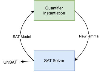
Figure 1: High-level architecture of cvc5. The techniques explained in Section 0.2, as well as our neural method (Section 2 and on), are particular cases of the top rectangle.

The default strategy of the solver is to first try the instantiations that use terms that were created earlier in the process (or were already in the input problem) — we refer to this as the age heuristic. For instance, for the ground part $\{p(c)\}$ and the quantifier $\forall x.\,q(f(x))$, the solver would instantiate by $c$ in the first round and by $f(c)$ in the second round. There is also the option to restrict the set of terms using the relevant domain, but in our experiments we turn this off. Disabling this option simplifies the integration of the machine learning component. The relevant domain option is also turned off in our machine learning experiments. When we say enumeration mode, we mean the pure enumeration without relevant domain. The enumeration procedure only produces one instantiation per quantified expression per round.
E-matching: In e-matching instantiation [14, 34], the solver looks for instantiations (substitutions) that yield an existing ground term, modulo equality. Since there may be many such terms, it only considers terms fitting a certain pattern—called trigger. Triggers may be provided by the user or generated by heuristics. As an example, consider the ground facts $\{a=f(17),p(a)\}$ and the quantifier formula $\forall x.\,\lnot p(f(x))\lor x<0$. The trigger $p(f(x))$ would cause e-matching to instantiate $x$ with $17$ because the term $p(f(17))$ fits the trigger and it is semantically equal to the existing term $p(a)$. This instantiation would yield the lemma $\lnot p(f(17))\lor 17<0$, which would give a contradiction with the ground facts. Preliminary investigations indicate that it is possible to use a similar machine learning setup as we used here to choose the triggers, but we leave it for future work here. Note that in contrast to the enumeration mode, e-matching may produce (potentially many) more than one instantiation per quantified expression per round. This difference in generative capacity becomes relevant in our experiments (Section 0.4).
Conflict-driven Instantiation: In conflict-driven quantifier instantiation [39], the solver looks for easily-detectable contradictions between the quantified part and the current model of the ground part; this reasoning is done modulo equality. As an example, consider a model $M$ that contains the facts $\{f(a)\neq g(b),b=h(a)\}$ and there is a quantified formula $\forall x.\,f(x)\neq g(h(x))$. Then, the solver quickly identifies that instantiating $x$ with $a$ causes a contradiction with $M$ and therefore, yielding the lemma $f(a)\neq g(h(a))$. Adding this lemma effectively excludes $M$ from further search. The method only looks for instantiations that guarantee a conflict with the current model and aims to be fast and is therefore inherently incomplete. This technique is part of the default settings of cvc5 and we can turn this off using --no-cbqi to arrive at a solver that uses only e-matching to instantiate.
Term Creation & Proliferation: In any of these strategies, new ground terms are created by the instantiations that they propose. For example, when a subterm $f(f(X))$ is instantiated with a constant $c$, the new ground term $f(f(c))$ is created, as well as its subterm $f(c)$, if this subterm did not already exist as a ground term in the problem. Potentially, this can create a lot of new terms, which make the problem of choosing terms for instantiations harder.

0.3 Neural Instantiation for cvc5

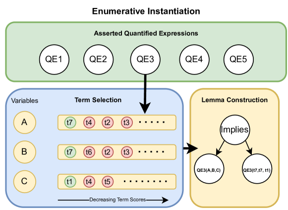
Figure 2: A schematic description of 1 instantiation within the enumerative instantiation procedure, which we heavily modify to create our neural solver. In the example a new ground lemma is created by instantiating the variables (A,B,C) in quantified expression 3 (QE3) with the ground terms (t7, t7, t1) respectively. In the default enumerative instantiation procedure, all quantified expressions are instantiated each round.

Setting: We build our neural guidance on top of the enumerative instantiation. This is because (i) enumeration is the conceptually simplest of the instantiation strategies, (ii) it is general and complete, and (iii) it allows fine-grained control over the instantiations (which can however also have the downsides mentioned in Section 0.1). That said, our current neural guidance method is not necessarily complete — it may be very unfair. This is exactly the objective of training a machine learning heuristic: we want to learn from previous proofs how we can push the solver to be biased towards choices similar to the ones that were previously successful. While in principle, it is possible to create the training data for the neural network also from the enumerative instantiation mode, we chose to use the e-matching procedure for that. This is because e-matching is much stronger on our dataset of FOL problems (see Section 0.4), providing us with much more training data. This is similar to the experiments done with the E and ENIGMA systems in [19], where the training data collected from the “smart” E strategies are used to train a guidance for a tabula rasa version of E.
GNN: While many different neural network methods can be used to guide automated theorem provers, a natural choice, based on the graph representation that cvc5 uses for the proof state, is the class of predictors called graph neural networks (GNNs) [43]. On a high level, GNNs represent each node in a graph with a vector of floating point numbers, and update these vectors using the vector representations of neighbouring nodes in the graph. By using optimization procedures, the GNN ‘learns’ to aggregate and update the node representations in such a way that at the end of several iterations of this neighbourhood-based updating procedure (usually called message passing), the node representations contain useful information to predict some relevant quantity. In our setting, these relevant quantities are: (i) scores for each quantified expression that represent whether this expression should be instantiated and (ii) scores for each pair of variables and terms that represent whether this particular variable should be instantiated with a particular term.

We implement a custom GNN using the C++ frontend of PyTorch [35]. ML-guided ATPs often use a separate GPU server [9, 21], to which multiple prover processes send their requests for advice. Here, we are however interested in a tight integration within cvc5, allowing the ML component to use only one CPU thread. This also means that no time is lost communicating and encoding/decoding between different processes and different programming languages.
GNN Proof State Representation: Each cvc5 state is represented as a graph. Its nodes represent cvc5 expressions. They have a kind, such as BOUND VARIABLE, APPLY, etc. Each of the kinds that cvc5 recognizes internally is given a separately trainable embedding (vector in $\mathbb{R}^{n}$) that serves as the initial embedding of each node before the message passing phase (see below). The edges between nodes are collected by modifying the DAG that cvc5 uses to represent the state. The GNN uses a bidirectional (cyclic) version of the DAG. For example, if we have a term $f(c)$, we have not only an edge from $f$ to $c$, but also an edge going the other way. We also use edge types to encode the argument ordering. For example, in $f(c,d)$ the edge from $f$ to $c$ has a different type than the edge from $f$ to $d$. We recognize up to 5 different argument positions, with the fifth used to represent all remaining positions. Each edge type has a numerical vector associated with it that is used to make it possible to distinguish argument order during the message passing procedure.
GNN Message Passing: For the message passing part of the GNN, a concatenation of the mean and max aggregation of neighbourhood messages is used. We have also implemented and tested the simpler mean and the more complicated attention-based aggregation methods. However, the mean-max version had the best balance of complexity and performance. Similarly, we tested the GNN with 2, 4, 10, 20 and 30 message passing layers, all with separate parameters. We found that 10 layers was a reasonable trade-off between the extra capability to fit the data and the execution speed within cvc5.

The different edge types are handled by adding a trainable vector $e$ (which differs for each of the recognized edge types) to each source node in an edge, before doing the neighbourhood accumulations. This method avoids having separate weight matrices and thus message passing rounds for each edge type [44], which could complicate and possibly slow down the computations. In addition, these edge vectors can be seen as analogous to the positional encodings often used in transformer architectures. The embedding update rules (for embedding size K) are as follows for a single node j with N neighbours labeled by i:

$$s_{t} =x_{t}+e_{\textrm{type}_{ij}}$$

$$x_{t+1}^{j} =\textrm{RELU}(W\cdot\textrm{CONCAT}(\frac{1}{N}\sum_{i=0}^{N}s_{t}^{i},\max(s_{t})))+x_{t}^{j},$$

where we compute a “source” vector $s$ for each neighbour i depending on the type of the edge from i to j. The MAX function returns a vector that is the elementwise maximum over all the neighbourhood vectors. The matrix $s_{t}$ has the shape $N\times K$ and $x_{t+1}^{j}$ is a vector of size $K$. $W$ is a linear transformation from dimensions $2K$ to $K$. CONCAT is a concatenation function that takes two vectors of size $K$ and returns a vector of size $2K$. RELU is the Rectified Linear Unit function, max(0, x), computed elementwise. The above is performed for each node and its neighbourhood, in each message passing step. Each message passing step uses its own weight matrix $W$. At the end of each message passing step, we add to each node the associated $x_{t}$ vector, which serves as residual connection, a way to easily propagate information unchanged through the layers, if it is useful. In our experiments, the embedding size K was set to 64.
GNN Output: To decide what the solver should do, we use two different outputs of the GNN (see also Figure 2): (i) probability distributions for each of the the top-level asserted quantified expressions, and (ii) for each variable a probability distribution over the terms of the right type, which we interpret as a probability that substituting this term in the variable leads to a useful instantiation. For output (i), note that we output a separate prediction for each quantified expression, which we can interpret as the probability that this quantified expression will be useful for the proof.

After the message passing steps, we have embeddings corresponding to each node in the graph. For the quantified expression selection task, we take all the nodes corresponding to the currently asserted top-level quantified expressions and apply a matrix transformation (a Linear layer) of size $K\times 1$ to each one, and use a sigmoid transformation to obtain a score between 0 and 1 for each one. Binary cross-entropy loss is used train the network to optimize the scores according to the data.

For the term ranking task, we take the embedding representing variables, and then for each variable the embeddings representing terms of the correct type. We apply separate trainable linear transformations (of size K to K) the term and variable embeddings and then compute dot products to obtain a distribution of term scores for each variable. We use a softmax transformation and cross-entropy loss to train the network to give high scores to variable-term substitutions occurring in the data.
Training Data Extraction: We have modified cvc5 to export the current proof state as a graph. For a particular problem, we extract for each solver round (Section 0.2 and Figure 1) the graph representation corresponding to the current proof state. To each such graph we also assign labels that indicate which quantified expressions and their instantiations were useful for the proof. In particular, our exporter labels instantiations as the correct answer as soon as the right ground terms become available. We also keep track of which instantiations were already done at a certain point in the run, so the GNN is not instructed to repeat instantiations. When there are multiple useful instantiations for the same quantified expression in a given proof state, we pick one at random. This is motivated by the enumerative instantiation mode’s default behavior, where we only instantiate each expression once in every round.
Training Details: For a given set of training problems, we might have many transitions for a single problem and few for another one. To balance this out, in each iteration over the dataset, we randomly sample one of the transitions associated with the known proof for each training problem. The Adam optimizer implemented in PyTorch was used with default parameters, except for the learning rate, which was set to 0.0001.

0.4 Experiments

All our experiments were run on a machine with Intel(R) Xeon(R) CPU E5-2698 v4 @ 2.20GHz CPU, 512GB RAM and NVIDIA Tesla V100 GPUs. The GPUs were used only for training the GNN. The trained neural models were always run on a single CPU when used for prediction inside cvc5. Our code and the trained GNN weights are available from our public repository.

0.4.1 Small Dataset

We first experimented with a small set of related problems extracted from the Mizar library. In particular, the MPTP2078 benchmark [1] has been used for several earlier AI/TP experiments [33, 27, 29]. To make this smaller benchmark compatible with the larger benchmark we ultimately use (see below), we update the problems there to their version corresponding to the MML version 1147. This yields 2172 problems. These problems were split into three different sets, the training set (80%), the development set (10%) and the holdout set (10%). The training set consists of problems where we are allowed to learn from solutions that we have, the development set consists of problems that we may tune the performance of our algorithm on and the holdout set is a set that is not used to tune parameters.

To collect training data for our approach, we ran our modified (Section 2) version of cvc5 in only e-matching mode. The states, as well as the instantiations done were logged. These were converted into training data using the procedure described in Section 2. We end up with 814 solved problems, from which we extract 1934 training transitions. The model was then trained for 2000 iterations over the dataset.

In Table 1, we show the results of running various versions of cvc5 for 10s on the development and holdout sets. The top 3 rows in the table correspond to a binary release of cvc5. The enumeration mode is observed to be a lot weaker on this dataset than e-matching. We also show a dry run, which is a run where we call the GNN to compute all the scores for quantified expressions (QEs) and term-variable combinations, but where we ignore those scores and simply use the default enumeration strategy’s suggestions. This allows us to gauge the slowdown caused by calling the GNN and its message passing and scoring procedures. While the 10s timeout can be seen as relatively short compared to the multi-minute timeouts used in competitions like SMTCOMP, it is indicative of the performance in a hammer-type setting.

We can use the scores (which are between 0 and 1 for each QE) predicted by the GNN in different ways. Here, we experimented with two procedures for the quantified expression scores: (i) QSampling, where we take the scores associated with each QE and interpret this as the probability of using this QE in this round. A sampling procedure decides, by drawing a random number between 0 and 1 and comparing with the score given, whether to instantiate this QE in this round. If the random number is higher than the score, we do not use the QE in this round. (ii) Threshold, where we compare the score to a threshold number and only instantiate the QEs with scores above the threshold. In our tuning phase (done on the development set), we found that a very low threshold value ($0.00001$) was the best setting for the Threshold variant. In general, false negatives (preventing a QE to be instantiated) seem to be a bigger problem for the solver than false positives. As in premise selection, having some extra QEs instantiated does not seem to be as problematic as omitting some necessary ones.

	Development	Holdout
Bcvc5 — default strategies	148	134
Bcvc5 — only e-matching	129	115
Bcvc5 — only enumeration	48	49
MLcvc5 — dry run	33	22
MLcvc5 — model (QSampling)	49	29
MLcvc5 — model (Threshold — 1 $\times$ 10-5)	54	35

Table 1: Number of problems solved by 10s runs on the devel and holdout parts of the small dataset. Bcvc5 is an unchanged binary release of cvc5. MLcvc5 is our modified version. Some of the changes cause a slowdown.

Comparing the ‘Bcvc5 — only enumeration’ and ‘MLcvc5 — dry run’ in Table 1 we see that the performance hit caused by calling the GNN is quite significant. However, we see that both on the development and holdout sets we do improve on the performance of the dry run. This means the predictions of the GNN are useful. Unfortunately, we are not able to improve on the binary version of enumeration on the holdout set. On the development set, we can improve on it by a few problems. The split between training, development and holdout was done randomly to prevent a bias in the different sets. However, several of the methods seem to have worse performance on the holdout set here. A larger selection of problems could help alleviate this. While these results indicate that the GNN can be useful for guidance of cvc5 in the enumeration mode, this training dataset might be too small to learn sufficiently strong GNN guidance.

0.4.2 Large Dataset (MPTP1147)

In the final evaluation we use the full MPTP 1147 benchmark, used previously in the Mizar40 [28] and Mizar60 [25] experiments. This dataset is more than 25x as large as the MPTP2078-induced subset (57917 problems in total). We use the train/devel/holdout split as defined in the previous work [25, 9]. Running on the training problems with the data collection mode of cvc5 with only e-matching active gives us 10945 solved problems, which we use to generate the training data. The model was trained for 150 iterations on this training dataset. After 150 epochs, the model has 82.9% accuracy on predicting the right terms for each variable on the training problems. For the quantified expression task, which scores the QEs between 0 and 1, 70.7% of useful quantified expressions are given a score above 0.5, while 88.3% of the non-useful quantified expressions are given a score below 0.5. While the model did not perfectly fit the training data, it has some capacity to learn the data.

	Development	Holdout
Bcvc5 — only e-matching	1096	1107
Bcvc5 — only enumeration	183	195
MLcvc5 — dry run	119	120
MLcvc5 — model (QSampling)	288	300
MLcvc5 — model (Threshold - 1x10-5, 1 inst)	324	336
MLcvc5 — model (Threshold - 1x10-5, 10 inst)	410	407

Table 2: MML1147: Number of problems solved by 10s runs. On both the development and the holdout sets the GNN-guided enumeration mode outperforms the unguided enumeration mode. Both the development and holdout set contain 2896 problems.

In Table 2, we show the development and holdout set performance of the ML-guided cvc5, along with various control experiments. We observe that the performance of the enumeration mode was improved by up to 72% ($336/195=1.723$) when we use the Threshold (1 inst) variant of our network. As a sanity check, we also ran a randomized dry run experiment on the development set, where we computed all the model scores, but used a randomly shuffled term ordering (instead of the age-based ordering for the usual dry run). This mode only solved 10 problems from the development set. These results taken together indicate that the network has learned a useful strategy from the e-matching generated training data, which it can apply in the ML enumeration mode.

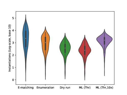
Figure 3: Violin plots of the number of instantiations performed in successful runs for Bcvc5 e-matching, Bcvc5 enumeration, dry run, the ML strategy with threshold 1e-5, and the ML strategy with 10x as many instantiations per quantifier per round. The white dots indicate the medians. The respective medians are 2235, 1026, 373.5, 250 and 1620.

Comparison of number of instantiations: While the runtime of all solvers was limited to 10s on 1 CPU, the various versions and settings of cvc5 can vary in terms of the absolute number of instantiations done within the same real time. The enumeration mode strives to perform at least 1 instantiation for each QE per round (Figures 1 and 2), and will not generally instantiate more than once for each QE in each round. E-matching, however, is not bound by this and will instantiate based on the number of pattern matches (which can be high). In Figure 3, we show the number of instantiations done in successful runs for five strategies. The median number for e-matching is an order of magnitude higher than in the ML strategy. E-matching is much more prolific than enumeration, and the ML strategy is less prolific in 10s than enumeration due to a combination of QEs that are not used and the GNN slowdown. The number of instantiations is of course also mediated by the time spent in computing the neural network’s predictions. This time varies heavily per problem and potentially per run, depending on the size of the initial problem and how much the graph grows each round (for example due to a lot of new lemmas and terms). In the successful runs on the MPTP1147 development set, there are neural network predictions that take below 40ms and ones that take more than 2400ms.
GNN run with multiple instantiations: The above analysis indicates that some difference in performance is due to the difference in the raw number of instantiations done. As we are already incurring the cost of computing the GNN advice, it might be the case that instantiation with multiple high-scoring tuples per round, instead of only 1 per QE as the original enumeration does, is a better use of the GNN advice. To test this, we ran a version of the ML mode that performs up to 10 instantiations per QE per round (see Table 2). This led to 407 solved holdout problems (again in 10s real time). This is a 109% increase compared to the unmodified enumeration mode ($407/195=2.09$).
Overlaps of sets: In Table 3, we show the set differences between the sets of solved problems for e-matching, enumeration and the best-performing ML setting on the holdout set. We observe that we can solve many problems that were not solved by the unguided enumeration mode, but that the e-matching mode is stronger than our method on this dataset.

	Bcvc5 - e-matching	Bcvc5 - enum	ML - (Thr-1x10-5, 10 inst)
Bcvc5 — e-matching	0	922	717
Bcvc5 — enum	10	0	34
ML — (Thr-1x10-5, 10 inst)	17	246	0

Table 3: Set differences in terms of number of solved problems on holdout set, row minus column. Example: the ML solves 246 problems that the enumeration mode does not.

0.5 Conclusion

In this work, we have shown that it is possible to improve cvc5’s enumerative instantiation by using an efficient graph neural network trained on many related problems. Our best result is 109% improvement in (realistically low) real time and with exactly the same hardware resources (i.e., a single CPU). This is done here so far in a first-order clausal setting without theories, however extensions to non-clausal SMT with theories should be mostly straightforward.

While e-matching largely dominates on first-order logic problems extracted from the Mizar Mathematical Library, on problems from the SMTLIB database, the enumeration procedure is much more competitive [26], and can even outperform e-matching on certain types of benchmarks. In principle, we can extend the current method to SMT problems, aside from the fact that the logging procedure that extracts training data from cvc5 runs needs to be modified. This could lead to some difficulties with tracing of instantiations, as it is not always clear how a term came to be (as the mechanism may be ‘hidden’ inside a theory component).

Future work will also investigate whether a better balance between the computation of the advice itself and the number of instantiation done based on this advice can be found. We may be under-utilizing the expensive advice of the GNN. Another direction of investigation will be the optimization of the speed of the neural network: it may be possible to use a much smaller neural network and still get reasonable predictions, but much faster. We will also investigate the generalization performance of the method. For example, testing the performance on problems extracted from other systems, such as Isabelle or Coq could be insightful. In general, our work shows for the first time that efficient real-time neural guidance for SMT solvers is possible.

0.6 Acknowledgements

This work was partially supported by the European Regional Development Fund under the Czech project AI&Reasoning no. CZ.02.1.01/0.0/0.0/15 003/0000466 (JP, JU), the European Union under the project ROBOPROX (reg. no. CZ.02.01.01/00/22_008/0004590) (MJ), Amazon Research Awards (JP, JU), by the Czech MEYS under the ERC CZ project POSTMAN no. LL1902 (JP, MJ, JU, JJ), ERC PoC grant no. 101156734 FormalWeb3 (JJ), and the EU ICT-48 2020 project TAILOR no. 952215 (JU).

References

- [1] Jesse Alama, Tom Heskes, Daniel Kühlwein, Evgeni Tsivtsivadze, and Josef Urban. Premise selection for mathematics by corpus analysis and kernel methods. J. Autom. Reasoning, 52(2):191–213, 2014.
- [2] Mislav Balunovic, Pavol Bielik, and Martin T. Vechev. Learning to solve SMT formulas. In NeurIPS, pages 10338–10349, 2018.
- [3] Kshitij Bansal, Sarah M. Loos, Markus N. Rabe, Christian Szegedy, and Stewart Wilcox. HOList: An environment for machine learning of higher order logic theorem proving. In ICML, volume 97 of Proceedings of Machine Learning Research, pages 454–463. PMLR, 2019.
- [4] Haniel Barbosa, Clark W. Barrett, Martin Brain, Gereon Kremer, Hanna Lachnitt, Makai Mann, Abdalrhman Mohamed, Mudathir Mohamed, Aina Niemetz, Andres Nötzli, Alex Ozdemir, Mathias Preiner, Andrew Reynolds, Ying Sheng, Cesare Tinelli, and Yoni Zohar. cvc5: A versatile and industrial-strength SMT solver. In TACAS (1), volume 13243. Springer, 2022.
- [5] Lasse Blaauwbroek, Josef Urban, and Herman Geuvers. Tactic learning and proving for the Coq proof assistant. In LPAR, volume 73 of EPiC Series in Computing, pages 138–150. EasyChair, 2020.
- [6] Jasmin Christian Blanchette, Sascha Böhme, and Lawrence C. Paulson. Extending sledgehammer with SMT solvers. J. Autom. Reason., 51(1):109–128, 2013.
- [7] Jasmin Christian Blanchette, Cezary Kaliszyk, Lawrence C. Paulson, and Josef Urban. Hammering towards QED. J. Formalized Reasoning, 9(1):101–148, 2016.
- [8] Jasmin Christian Blanchette, Daniel El Ouraoui, Pascal Fontaine, and Cezary Kaliszyk. Machine Learning for Instance Selection in SMT Solving. In AITP 2019 - 4th Conference on Artificial Intelligence and Theorem Proving, Obergurgl, Austria, April 2019.
- [9] Karel Chvalovský, Konstantin Korovin, Jelle Piepenbrock, and Josef Urban. Guiding an instantiation prover with graph neural networks. In LPAR, volume 94 of EPiC Series in Computing, pages 112–123. EasyChair, 2023.
- [10] M. Davis and H. Putnam. A Computing Procedure for Quantification Theory. Journal of the ACM, 7(1):215–215, 1960.
- [11] Martin Davis. The early history of automated deduction. In Handbook of Automated Reasoning, pages 3–15. Elsevier and MIT Press, 2001.
- [12] Leonardo Mendonça de Moura and Nikolaj Bjørner. Z3: An Efficient SMT Solver. In C. R. Ramakrishnan and Jakob Rehof, editors, TACAS, volume 4963 of LNCS, pages 337–340. Springer, 2008.
- [13] Martin Desharnais, Petar Vukmirovic, Jasmin Blanchette, and Makarius Wenzel. Seventeen provers under the hammer. In ITP, volume 237 of LIPIcs, pages 8:1–8:18. Schloss Dagstuhl - Leibniz-Zentrum für Informatik, 2022.
- [14] David Detlefs, Greg Nelson, and James B Saxe. Simplify: a theorem prover for program checking. Journal of the ACM (JACM), 52(3):365–473, 2005.
- [15] Daniel El Ouraoui. Méthodes pour le raisonnement d’ordre supérieur dans SMT, Chapter 5. PhD thesis, Université de Lorraine, 2021.
- [16] Harald Ganzinger and Konstantin Korovin. New directions in instantiation-based theorem proving. In 18th IEEE Symposium on Logic in Computer Science (LICS 2003), 22-25 June 2003, Ottawa, Canada, Proceedings, pages 55–64. IEEE Computer Society, 2003.
- [17] Thibault Gauthier, Cezary Kaliszyk, and Josef Urban. TacticToe: Learning to reason with HOL4 tactics. In LPAR-21, 21st International Conference on Logic for Programming, Artificial Intelligence and Reasoning, Maun, Botswana, May 7-12, 2017, pages 125–143, 2017.
- [18] Thibault Gauthier, Cezary Kaliszyk, Josef Urban, Ramana Kumar, and Michael Norrish. Tactictoe: Learning to prove with tactics. J. Autom. Reason., 65(2):257–286, 2021.
- [19] Zarathustra Amadeus Goertzel. Make E smart again (short paper). In IJCAR (2), volume 12167 of Lecture Notes in Computer Science, pages 408–415. Springer, 2020.
- [20] Zarathustra Amadeus Goertzel, Karel Chvalovský, Jan Jakubuv, Miroslav Olsák, and Josef Urban. Fast and slow enigmas and parental guidance. In Boris Konev and Giles Reger, editors, Frontiers of Combining Systems - 13th International Symposium, FroCoS 2021, Birmingham, UK, September 8-10, 2021, Proceedings, volume 12941 of Lecture Notes in Computer Science, pages 173–191. Springer, 2021.
- [21] Zarathustra Amadeus Goertzel, Jan Jakubův, Cezary Kaliszyk, Miroslav Olsák, Jelle Piepenbrock, and Josef Urban. The Isabelle ENIGMA. In ITP, volume 237 of LIPIcs, pages 16:1–16:21. Schloss Dagstuhl - Leibniz-Zentrum für Informatik, 2022.
- [22] Jacques Herbrand. Recherches sur la théorie de la démonstration. Doctorat d’état, La Faculté des Sciences de Paris, 1930.
- [23] Jan Jakubův, Karel Chvalovský, Miroslav Olsák, Bartosz Piotrowski, Martin Suda, and Josef Urban. ENIGMA anonymous: Symbol-independent inference guiding machine (system description). In Nicolas Peltier and Viorica Sofronie-Stokkermans, editors, Automated Reasoning - 10th International Joint Conference, IJCAR 2020, Paris, France, July 1-4, 2020, Proceedings, Part II, volume 12167 of Lecture Notes in Computer Science, pages 448–463. Springer, 2020.
- [24] Jan Jakubův and Josef Urban. ENIGMA: efficient learning-based inference guiding machine. In Herman Geuvers, Matthew England, Osman Hasan, Florian Rabe, and Olaf Teschke, editors, Intelligent Computer Mathematics - 10th International Conference, CICM 2017, Edinburgh, UK, July 17-21, 2017, Proceedings, volume 10383 of Lecture Notes in Computer Science, pages 292–302. Springer, 2017.
- [25] Jan Jakubuv, Karel Chvalovský, Zarathustra Amadeus Goertzel, Cezary Kaliszyk, Mirek Olsák, Bartosz Piotrowski, Stephan Schulz, Martin Suda, and Josef Urban. MizAR 60 for Mizar 50. In ITP, volume 268 of LIPIcs, pages 19:1–19:22. Schloss Dagstuhl - Leibniz-Zentrum für Informatik, 2023.
- [26] Mikoláš Janota, Haniel Barbosa, Pascal Fontaine, and Andrew Reynolds. Fair and adventurous enumeration of quantifier instantiations. In 2021 Formal Methods in Computer Aided Design (FMCAD), pages 256–260. IEEE, 2021.
- [27] Cezary Kaliszyk and Josef Urban. FEMaLeCoP: Fairly efficient machine learning connection prover. In Martin Davis, Ansgar Fehnker, Annabelle McIver, and Andrei Voronkov, editors, Logic for Programming, Artificial Intelligence, and Reasoning - 20th International Conference, LPAR-20 2015, Suva, Fiji, November 24-28, 2015, Proceedings, volume 9450 of Lecture Notes in Computer Science, pages 88–96. Springer, 2015.
- [28] Cezary Kaliszyk and Josef Urban. MizAR 40 for Mizar 40. J. Autom. Reasoning, 55(3):245–256, 2015.
- [29] Cezary Kaliszyk, Josef Urban, Henryk Michalewski, and Miroslav Olsák. Reinforcement learning of theorem proving. In Advances in Neural Information Processing Systems 31: Annual Conference on Neural Information Processing Systems 2018, NeurIPS 2018, 3-8 December 2018, Montréal, Canada., pages 8836–8847, 2018.
- [30] Ekaterina Komendantskaya, Jónathan Heras, and Gudmund Grov. Machine learning in Proof General: Interfacing interfaces. In UITP, volume 118 of EPTCS, pages 15–41, 2012.
- [31] Konstantin Korovin. iProver - an instantiation-based theorem prover for first-order logic (system description). In Alessandro Armando, Peter Baumgartner, and Gilles Dowek, editors, Automated Reasoning, 4th International Joint Conference, IJCAR 2008, Sydney, Australia, August 12-15, 2008, Proceedings, volume 5195 of Lecture Notes in Computer Science, pages 292–298. Springer, 2008.
- [32] Laura Kovács and Andrei Voronkov. First-order theorem proving and Vampire. In Natasha Sharygina and Helmut Veith, editors, CAV, volume 8044 of LNCS, pages 1–35. Springer, 2013.
- [33] Daniel Kühlwein, Twan van Laarhoven, Evgeni Tsivtsivadze, Josef Urban, and Tom Heskes. Overview and evaluation of premise selection techniques for large theory mathematics. In Bernhard Gramlich, Dale Miller, and Uli Sattler, editors, IJCAR, volume 7364 of LNCS, pages 378–392. Springer, 2012.
- [34] Michał Moskal, Jakub Łopuszański, and Joseph R Kiniry. E-matching for fun and profit. Electronic Notes in Theoretical Computer Science, 198(2):19–35, 2008.
- [35] Adam Paszke, Sam Gross, Francisco Massa, Adam Lerer, James Bradbury, Gregory Chanan, Trevor Killeen, Zeming Lin, Natalia Gimelshein, Luca Antiga, et al. Pytorch: An imperative style, high-performance deep learning library. Advances in neural information processing systems, 32, 2019.
- [36] Nikhil Pimpalkhare, Federico Mora, Elizabeth Polgreen, and Sanjit A. Seshia. MedleySolver: Online SMT algorithm selection. In Chu-Min Li and Felip Manyà, editors, Theory and Applications of Satisfiability Testing – SAT 2021, pages 453–470, Cham, 2021. Springer International Publishing.
- [37] Michael Rawson and Giles Reger. lazyCoP: Lazy paramodulation meets neurally guided search. In TABLEAUX, volume 12842 of Lecture Notes in Computer Science, pages 187–199. Springer, 2021.
- [38] Andrew Reynolds, Haniel Barbosa, and Pascal Fontaine. Revisiting enumerative instantiation. In Tools and Algorithms for the Construction and Analysis of Systems: 24th International Conference, TACAS 2018, Held as Part of the European Joint Conferences on Theory and Practice of Software, ETAPS 2018, Thessaloniki, Greece, April 14-20, 2018, Proceedings, Part II 24, pages 112–131. Springer, 2018.
- [39] Andrew Reynolds, Cesare Tinelli, and Leonardo Mendonça de Moura. Finding conflicting instances of quantified formulas in SMT. In Formal Methods in Computer-Aided Design, FMCAD 2014, Lausanne, Switzerland, October 21-24, 2014, pages 195–202. IEEE, 2014.
- [40] Jason Rute, Miroslav Olsák, Lasse Blaauwbroek, Fidel Ivan Schaposnik Massolo, Jelle Piepenbrock, and Vasily Pestun. Graph2tac: Learning hierarchical representations of math concepts in theorem proving. CoRR, abs/2401.02949, 2024.
- [41] Mikoláš Janota, Jelle Piepenbrock, and Bartosz Piotrowski. Towards learning quantifier instantiation in SMT. In Kuldeep S. Meel and Ofer Strichman, editors, 25th International Conference on Theory and Applications of Satisfiability Testing, SAT 2022, August 2-5, 2022, Haifa, Israel, volume 236 of LIPIcs, pages 7:1–7:18. Schloss Dagstuhl - Leibniz-Zentrum für Informatik, 2022.
- [42] Alex Sanchez-Stern, Yousef Alhessi, Lawrence K. Saul, and Sorin Lerner. Generating correctness proofs with neural networks. CoRR, abs/1907.07794, 2019.
- [43] Franco Scarselli, Marco Gori, Ah Chung Tsoi, Markus Hagenbuchner, and Gabriele Monfardini. The graph neural network model. IEEE transactions on neural networks, 20(1):61–80, 2008.
- [44] Michael Schlichtkrull, Thomas N Kipf, Peter Bloem, Rianne Van Den Berg, Ivan Titov, and Max Welling. Modeling relational data with graph convolutional networks. In The Semantic Web: 15th International Conference, ESWC 2018, Heraklion, Crete, Greece, June 3–7, 2018, Proceedings 15, pages 593–607. Springer, 2018.
- [45] S. Schulz. A Comparison of Different Techniques for Grounding Near-Propositional CNF Formulae. In S. Haller and G. Simmons, editors, Proc. of the 15th FLAIRS, Pensacola, pages 72–76. AAAI Press, 2002.
- [46] Stephan Schulz. System description: E 1.8. In Kenneth L. McMillan, Aart Middeldorp, and Andrei Voronkov, editors, LPAR, volume 8312 of LNCS, pages 735–743. Springer, 2013.
- [47] Joseph Scott, Aina Niemetz, Mathias Preiner, Saeed Nejati, and Vijay Ganesh. MachSMT: A machine learning-based algorithm selector for SMT solvers. In Jan Friso Groote and Kim Guldstrand Larsen, editors, Tools and Algorithms for the Construction and Analysis of Systems, pages 303–325, Cham, 2021. Springer International Publishing.
- [48] Daniel Selsam and Nikolaj Bjørner. Guiding high-performance sat solvers with unsat-core predictions. In Theory and Applications of Satisfiability Testing–SAT 2019: 22nd International Conference, SAT 2019, Lisbon, Portugal, July 9–12, 2019, Proceedings 22, pages 336–353. Springer, 2019.
- [49] Martin Suda. Improving enigma-style clause selection while learning from history. In CADE, volume 12699 of Lecture Notes in Computer Science, pages 543–561. Springer, 2021.
- [50] Josef Urban, Jiří Vyskočil, and Petr Štěpánek. MaLeCoP: Machine learning connection prover. In Kai Brünnler and George Metcalfe, editors, TABLEAUX, volume 6793 of LNCS, pages 263–277. Springer, 2011.
- [51] Zsolt Zombori, Josef Urban, and Miroslav Olsák. The role of entropy in guiding a connection prover. In TABLEAUX, volume 12842 of Lecture Notes in Computer Science, pages 218–235. Springer, 2021.