Maxwell-$f(Q)$ theory

Abstract

Exploring the four-dimensional AdS black hole is crucial within the framework of the AdS/CFT correspondence. In this research, considering the charged scenario, we investigate the four-dimensional stationary and rotating AdS solutions in the framework of the $f(Q)$ gravitational theory. Our emphasis is on the power-law ansatz, which is consistent with observations and is deemed the most viable. Because this solution does not have an uncharged version or relate to general relativity, it falls into a new category, which derives its features from changes in non-metricity and incorporates the Maxwell domain. We analyze the singularities of such a solution, computing all the quantities of different curvature and non-metricity invariants. Our results indicate the presence of a central singularity, albeit with a softer nature compared to standard non-metricity or Einstein general relativity, attributed to the influence of the effect of $f(Q)$. We examine several physical characteristics of black holes from a thermodynamics perspective and demonstrate the existence of an outer event horizon in addition to the inner Cauchy horizons. However, under the conditions of a sufficiently large electric charge, a naked singularity emerges. Finally, we derive a class of rotating black hole in four-dimensional $f(Q)$ gravity that are asymptotically anti-de Sitter charged.

I Introduction

Over the past few years, there has been considerable debate about gravitational theories that incorporate non-metricity Nester and Yo (1999); Beltrán Jiménez et al. (2018a, 2019); Rünkla and Vilson (2018); Beltrán Jiménez et al. (2020). These gravitational theories use a quantity called the non-metricity scalar $Q$ and follow the Palatini formalism. This approach treats the connection, along with the metric, as independent variables. When the Riemann tensor and torsion tensor for the connection are set to zero, it is found that the connection can be described using four scalar fields Blixt et al. (2023); Beltrán Jiménez and Koivisto (2022); Adak (2018); Tomonari and Bahamonde (2023). Furthermore, by choosing certain scalar fields, one can set the connection to zero, a condition known as the coincident gauge D’Ambrosio et al. (2022). In this scenario, the metric becomes the sole dynamic variable in the theory. It has been shown that in the coincident gauge, a theory with a linear action, denoted as $Q$, is equivalent to general relativity (GR). This equivalence is termed as Symmetric Teleparallel Equivalent to GR (STEGR) Beltrán Jiménez et al. (2018b); Quiros (2022).

Teleparallelism is a widely recognized concept in gravitational theory that operates independently of curvature. In this framework, the torsion scalar $T$ is considered as the fundamental quantity Maluf (2013); Aldrovandi and Pereira (2013); Cai et al. (2016). Choosing the Weitzenböck connection and using the coincident gauge in STEGR results in the elimination of the spin connection, leaving only the tetrad as the dynamic variable. The theory with an action linear to $T$ is equivalent to GR and is called teleparallel equivalent to GR (TEGR) Maluf (2013); Krššák and Saridakis (2016). In non-metricity gravity, unlike teleparallelism, we use “symmetric” teleparallelism to meet the torsionless requirement, which requires a symmetric affine connection. Similarly to how we extend GR to $f(R)$ gravity Nashed (2018), which involves a function of the curvature scalar, TEGR Nashed et al. (2019); Nashed and Saridakis (2020), and STEGR have also been extended to $f(T)$ and $f(Q)$ gravity, respectively. These extensions incorporate arbitrary functions of $T$ and $Q$ in their actions Bahamonde et al. (2015); Cai et al. (2016); Krššák and Saridakis (2016); Bahamonde et al. (2023); Hu et al. (2023); Heisenberg (2019); Beltrán Jiménez et al. (2020); Harko et al. (2018); Järv et al. (2018); Rünkla and Vilson (2018); Capozziello et al. (2022, 2023). These theories have been extensively studied in the context of modified gravity. By introducing new degrees of freedom (DOF) through torsion or non-metricity, a range of fascinating phenomena has been revealed, especially in cosmological models Hu et al. (2024); Qiu et al. (2019); Nájera and Fajardo (2022); Li and Zhao (2022); Khyllep et al. (2021); Casalino et al. (2021); Sharma and Sur (2021, 2022, 2023); Mandal et al. (2020a, b); Mandal and Sahoo (2021); Arora and Sahoo (2022); Gadbail et al. (2022); Paliathanasis (2024, 2023a); Dimakis et al. (2022); Paliathanasis (2023b), studies have explored solutions related to black holes Wang et al. (2022); Lin and Zhai (2021); D’Ambrosio et al. (2022); Bahamonde et al. (2022); Calzá and Sebastiani (2023), as well as gravitational waves Hohmann et al. (2018, 2019); Soudi et al. (2019); Abedi and Capozziello (2018). In D’Ambrosio et al. (2022) authors derived many perturbative spherically symmetric solutions using different forms of $f(Q)$.

Recently, there has been growing interest in the number of DOF in $f(Q)$ gravity Hu et al. (2022); D’Ambrosio et al. (2023); Tomonari and Bahamonde (2023); Heisenberg (2024); Paliathanasis et al. (2024); Dimakis et al. (2021). In a prior investigation by Hu et al. Hu et al. (2022), they showed that coincident $f(Q)$ gravity has eight DOFs, with the scalar mode unable to propagate. However, it’s important to mention that the conclusions from Ref. Hu et al. (2022) have sparked controversy and are currently being actively discussed (for more details, c.f. D’Ambrosio et al. (2023); Tomonari and Bahamonde (2023)). However, the current literature concerning Hamiltonian analysis heavily relies on a specific gauge called the coincident gauge D’Ambrosio et al. (2023). It is essential to confirm that there are no ghost modes with negative kinetic energy among the physical DOFs without resorting to gauge fixing. This study primarily concentrates on a charged black hole solution within the cubic form of $f(Q)$ theory. Additionally, we examine the construction of this solution by studying its invariants as well as thermodynamic quantities.

The structure of this paper is outlined as follows: In Section II, we introduce the basic geometrical framework of charged $f(Q)$ gravitational theory. In Section III, we employ cylindrical coordinates (t, r, $\xi_{1}$, and $\xi_{2}$) to apply the charged field equation of $f(Q)$ to a four-dimensional line element with two unknown functions. In Section III, we present both charged and uncharged black holes within the cubic form of $f(Q)$. Furthermore, we discuss the interaction between the physics of the charged black hole and its singularity in the same section. In Section IV, we propose a new rotating black hole using the cubic form of the $f(Q)$ gravitational theory. Section V is dedicated to calculate the entropy, Hawking temperature, and heat capacity to analyze the thermodynamic behavior of the charged black hole. Finally, in Section VI, we conclude this study and discuss the findings of our investigation.

II Maxwell-$f(Q)$ theory

Weyl geometry represents a substantial advancement beyond Riemannian geometry, forming the mathematical underpinning of GR. In Weyl geometry, when a vector undergoes parallel transport along a closed path, it not only alters its direction but also its magnitude. Consequently, in the framework of Weyl’s the metric tensor’s covariant derivative is not zero, and this feature can be mathematically represented by a recently introduced geometric quantity known as non-metricity, which is represented by the letter $Q$. Hence, the covariant derivative of the metric tensor $g_{\mu\nu}$ with respect to the general affine connection, $\overline{\Gamma}_{\leavevmode\nobreak\ \mu\gamma}^{\sigma}$, yields the definition of the non-metricity tensor $Q_{\gamma\mu\nu}$, and it can be formulated as Beltrán Jiménez et al. (2018b, 2020, a),

$$Q_{\gamma\mu\nu}=-\nabla_{\gamma}g_{\mu\nu}=-\frac{\partial g_{\mu\nu}}{\partial x^{\gamma}}+g_{\nu\sigma}\overline{\Gamma}_{\leavevmode\nobreak\ \mu\gamma}^{\sigma}+g_{\sigma\mu}\overline{\Gamma}_{\leavevmode\nobreak\ \nu\gamma}^{\sigma}.$$ (1)

Under these circumstances, the Weyl connection that characterizes the general affine connection can be divided into two separate parts, which are as follows:

$$\overline{\Gamma}_{\ \mu\nu}^{\gamma}=\left\{{}^{\,\alpha}_{\mu\nu}\right\}+L_{\ \mu\nu}^{\gamma}.$$ (2)

In Eq. (2), the Levi-Civita connection for the metric $g_{\mu\nu}$ is represented by the first term which and defined as:

$$\left\{{}^{\,\alpha}_{\mu\nu}\right\}\equiv\frac{1}{2}g^{\gamma\sigma}\left(\frac{\partial g_{\sigma\nu}}{\partial x^{\mu}}+\frac{\partial g_{\sigma\mu}}{\partial x^{\nu}}-\frac{\partial g_{\mu\nu}}{\partial x^{\sigma}}\right).$$ (3)

Moreover, the second term in Eq. (2) expresses the tensor of disformation resulting from the non-metricity that can be expressed in the following manner:

$$L_{\leavevmode\nobreak\ \mu\nu}^{\gamma}\equiv\frac{1}{2}g^{\gamma\sigma}\left(Q_{\nu\mu\sigma}+Q_{\mu\nu\sigma}-Q_{\gamma\mu\nu}\right)=L_{\leavevmode\nobreak\ \nu\mu}^{\gamma}.$$ (4)

Moreover, by contracting the non-metricity tensor we derive the non-metricity scalar from the disformation tensor as:

$$Q\equiv-g^{\mu\nu}\left(L_{\ \ \beta\mu}^{\alpha}L_{\ \ \nu\alpha}^{\beta}-L_{\ \ \beta\alpha}^{\alpha}L_{\ \ \mu\nu}^{\beta}\right).$$ (5)

Expansion of Weyl geometry to include space-time torsion results in the Weyl-Cartan geometries having torsion. In the geometry of Weyl-Cartan, the general affine connection could be divided into two separate components:

$$\overline{\Gamma}_{\ \mu\nu}^{\gamma}=\left\{{}^{\,\alpha}_{\mu\nu}\right\}+K_{\ \mu\nu}^{\gamma}.$$ (6)

In Eq. (6), the part on the right-hand side shows contortion which is described by the torsion tensor $T_{\ \mu\nu}^{\gamma}$ It is defined as $2\overline{\Gamma}_{\leavevmode\nobreak\ [\mu\nu]}^{\gamma}$ and can have the following form:

$$K_{\ \mu\nu}^{\gamma}\equiv\frac{1}{2}g^{\gamma\sigma}\left(T_{\mu\sigma\nu}+T_{\nu\sigma\mu}+T_{\sigma\mu\nu}\right).$$ (7)

Moreover, the connection between the curvature tensors $R_{\sigma\mu\nu}^{\rho}$ and $\mathring{R}{\sigma\mu\nu}^{\rho}$ associated with the connections $\overline{\Gamma}{\ \mu\nu}^{\gamma}$ and $\Gamma_{\ \mu\nu}^{\gamma}$ is:

$$R_{\sigma\mu\nu}^{\rho}=\mathring{R}_{\sigma\mu\nu}^{\rho}+\mathring{\nabla}_{\mu}L_{\nu\sigma}^{\rho}-\mathring{\nabla}_{\nu}L_{\mu\sigma}^{\rho}+L_{\mu\lambda}^{\rho}L_{\nu\sigma}^{\lambda}-L_{\nu\lambda}^{\rho}L_{\mu\sigma}^{\lambda},$$ (8)

$$R_{\sigma\nu}=\mathring{R}_{\sigma\nu}+\frac{1}{2}\mathring{\nabla}_{\nu}Q_{\sigma}+\mathring{\nabla}_{\rho}L_{\nu\sigma}^{\rho}-\frac{1}{2}Q_{\lambda}L_{\nu\sigma}^{\lambda}-L_{\sigma\lambda}^{\rho}L_{\rho\sigma}^{\lambda},$$ (9)

and the relationship regarding Ricci scalar has the from:

$$R=\mathring{R}+\mathring{\nabla}_{\lambda}Q^{\lambda}-\mathring{\nabla}_{\lambda}\tilde{Q}^{\lambda}-\frac{1}{4}Q_{\lambda}Q^{\lambda}+\frac{1}{2}Q_{\lambda}\tilde{Q}^{\lambda}-L_{\rho\nu\lambda}L^{\lambda\rho\nu}.$$ (10)

withe $\mathring{\nabla}$ represents the operator of the covariant derivative associated with the Levi-Civita relationship $\Gamma_{\ \mu\nu}^{\gamma}$. The general affine connection in STEGR is constrained by the lack of curvature and torsion requirements. For a Riemann tensor $R_{\sigma\mu\nu}^{\rho}\left(\overline{\Gamma}\right)$ to be curvature-free it must has a vanishing value. The parallel transport performed by the covariant derivative $\nabla$ and its affine connection $\overline{\Gamma}_{\ \mu\nu}^{\gamma}$ becomes path-independent when the Riemann tensor vanishes. This theory, STEGR, implies that $T_{\ \mu\nu}^{\gamma}=0$ and that the connection must be torsionless in addition to requiring zero curvature. In this theory gravitational effects are entirely attributed to the non-metricity. when the torsion tensor vanishes this yields to symmetric lower indices for the general affine connection.

Now if we start from a teleparallel condition, which corresponds to a variety with a plane geometry characterizing a pure inertial connection, it is possible to perform a gauge transformation of the linear group ${GL}(4,{{R}})$ parameterized by $\Lambda_{\phantom{\alpha}\mu}^{\alpha}$ Beltrán Jiménez et al. (2019, 2020),

$$\Gamma_{\phantom{\alpha}\mu\nu}^{\alpha}=\left(\Lambda^{-1}\right)_{\phantom{\alpha}\beta}^{\alpha}\partial_{[\mu}\Lambda_{\phantom{\alpha}\nu]}^{\beta}.$$ (11)

So we can write that the most general possible connection, through the general element of ${\textrm{G}L}(4,{{R}})$, which is parameterized by the transformation of $\Lambda_{\phantom{\alpha}\mu}^{\alpha}=\partial_{\mu}\xi^{\alpha}$, where $\xi^{\alpha}$ is an arbitrary vector field,

$$\Gamma_{\phantom{\alpha}\mu\nu}^{\alpha}=\frac{\partial x^{\alpha}}{\partial\xi^{\rho}}\partial_{\mu}\partial_{\nu}\xi^{\rho}.$$ (12)

This result shows us that the connection can be removed by a coordinate transformation. The transformation that results in the connection (12) being removed is called gauge coincident Beltrán Jiménez et al. (2018a).

Consequently, from the coincident gauge we have that the non-metricity tensor defined by (1) becomes,

$$Q_{\beta\mu\nu}\equiv\partial_{\beta}g_{\mu\nu}.$$ (13)

In this study, we use the coincident gauge to compute our solution.

Finally, the gravity action of $f(Q)$ can be constructed as follows using the non-metricity scalar Beltrán Jiménez et al. (2018b):

$$S=-\frac{1}{2\kappa^{2}}\int_{\mathcal{M}}f({Q})\sqrt{-g}d^{4}x+\int\sqrt{-g}{\mathcal{L}}_{em}\leavevmode\nobreak\ d^{4}x\,.$$ (14)

Here, the space-time manifold, the covariant metric tensor, and the determinant are denoted by $g$, $g_{\mu\nu}$, and $\mathcal{M}$, respectively. The generic functional form of the non-metricity scalar ${Q}$ is represented by the function $f({Q})$. Here $\kappa=8\pi$ defines $\kappa$ in relativistic units, i.e., $c=G=1$, where the gravitational constant and the speed of light are identical. The Maxwell field Lagrangian is represented by ${\mathcal{L}}_{em}=-\frac{1}{2}{F}\wedge^{\star}{F}$ in Eq. (14), where $F=dA$ and $A=A_{\mu}dx^{\mu}$ is the 1-form of the electromagnetic potential Awad et al. (2017). Just like $f(R)$ gravity, $f(Q)$ gravity also results in deviations from Einstein GR. As an illustration, by setting the $f(Q)=Q$, we recover the STEGR. From the non-metricity tensor, we can extract only two independent traces because of the symmetry of the metric tensor $g_{\mu\nu}$, $Q_{\gamma\mu\nu}$,

$$Q_{\gamma}\equiv Q_{\gamma\ \ \ \mu}^{\ \ \mu},\ \ \ \ \tilde{Q}_{\gamma}\equiv Q_{\ \ \gamma\mu}^{\mu}.$$ (15)

Furthermore, it would be helpful to present the conjugate defining non-metricity as:

$$\hskip-14.22636ptP_{\ \ \mu\nu}^{\gamma}\equiv\frac{1}{4}\bigg{[}-Q_{\ \ \mu\nu}^{\gamma}+2Q_{\left(\mu\ \ \ \nu\right)}^{\ \ \ \gamma}+Q^{\gamma}g_{\mu\nu}-\widetilde{Q}^{\gamma}g_{\mu\nu}-\delta_{\ \ (\mu}^{\gamma}Q_{\nu)}\bigg{]}=-\frac{1}{2}L_{\ \ \mu\nu}^{\gamma}+\frac{1}{4}\left(Q^{\gamma}-\widetilde{Q}^{\gamma}\right)g_{\mu\nu}-\frac{1}{4}\delta_{\ \ (\mu}^{\gamma}Q_{\nu)}.$$ (16)

The non-metricity scalar is calculated as follows:

$$Q=-Q_{\gamma\mu\nu}P^{\gamma\mu\nu}=-\frac{1}{4}\big{(}-Q^{\gamma\nu\rho}Q_{\gamma\nu\rho}+2Q^{\gamma\nu\rho}Q_{\rho\gamma\nu}-2Q^{\rho}\tilde{Q}_{\rho}+Q^{\rho}Q_{\rho}\big{)}.$$ (17)

When deriving the field equations of the theory, one performs separate variations with respect to the metric and matter fields of Eq. (14) that yield Heisenberg (2024):

$$\zeta_{\mu\nu}=\frac{2}{\sqrt{-g}}\nabla_{\alpha}\left(\sqrt{-g}f_{Q}P^{\alpha}_{\;\;\mu\nu}\right)+\frac{1}{2}g_{\mu\nu}f+f_{Q}\left(P_{\mu\alpha\beta}{Q}^{\;\;\alpha\beta}_{\nu}-2P_{\alpha\beta\mu}{Q}^{\;\;\alpha\beta}_{\nu}\right)+\kappa^{2}\frac{1}{2}\kappa{{{\mathcal{T}}^{{}^{{}^{{\!\!\!\!\scriptstyle{em}}}}}}}_{\mu\nu}$$

$$\partial_{\nu}\left(\sqrt{-g}F^{\mu\nu}\right)=0\;,$$ (18)

The variation of Eq. (14) with respect to the connection yields:

$${\nabla^{\mu}\nabla^{\nu}\left(\sqrt{-g}f_{Q}P^{\alpha}_{\;\;\mu\nu}\right)=0}\,.$$ (19)

In this study, ${\mathcal{T}_{\mu}^{\nu}{}^{{}^{\text{em}}}}$ denotes the tensor characterizing the electromagnetic field’s energy-momentum, which is figured as:

$${{{\mathcal{T}}^{{}^{{}^{{\!\!\!\!\scriptstyle{em}}}}}}}^{\nu}_{\mu}=F_{\mu\alpha}F^{\nu\alpha}-\frac{1}{4}\delta_{\mu}{}^{\nu}F_{\alpha\beta}F^{\alpha\beta}.$$

In Eq. (ref1st EOM), $f$ is defined as $f({Q})$, and $f_{Q}$ is its first derivative with respect to ${Q}$. It is worth noting that the matter Lagrangian density is varied independently regarding the connection, resulting in the absence of hyper-momentum. Furthermore, as is widely recognized, the outcomes of GR (in the framework of scalar-tensor extended GR, STEGR) are obtained by setting $f({Q})={Q}$. Consequently, the Lagrangian density takes the form $\mathcal{L}=-\frac{{Q}}{2\kappa^{2}}+\mathcal{L}_{m}$, where $f_{Q}=\frac{df}{dQ}$.

III Solution of anti-de-Sitter black hole

Next, we will derive a solution of AdS charged black hole within $f(Q)$ theory, with a specific emphasis on four-dimensional spacetime. We utilize cylindrical coordinates ($t$, $r$, $\xi_{1}$, $\xi_{2}$), with the ranges $0\leq r<\infty$, $-\infty<t<\infty$, and $0\leq\xi_{i}<2\pi$, $i=1,2$ . Within this context, let’s use the following metric:

$$ds^{2}=S(r)dt^{2}-\frac{1}{S_{1}(r)}dr^{2}-r^{2}\left(d\xi^{2}_{1}+d\xi^{2}_{2}\right)\,.$$ (20)

The radial coordinate $r$ is the only variable that fixes the functions $S(r)$ and $S_{1}(r)$. Notably, the metric (20) includes flat sections rather than spherical or hyperbolic ones, indicating that it is not entirely general. It is shown in D’Ambrosio et al. (2022), that if we start from a general metric-affine geometry, one can construct the most general static and spherically symmetric forms of the metric and the affine connection. Then the uses of these symmetry-reduced geometric objects to prove that the field equations of $f(Q)$ gravity admit GR solutions and other solutions beyond GR. This is contrary to what has been known in the literature. In this study we focus on the metric (20) to obtain a solution that is different from GR where $Q$ has a non-constant value and $f(Q)$ is not linear.

For this reason, we focus on the metric (20) in order to obtain novel solutions where we can derive the non-constant value of $Q$ and the non-linear form of $f(Q)$. When we plug this metric form into the equation for non-metricity, we get:

$$Q=-{\frac{2S_{1}\left(rS^{\prime}+S\right)}{{r}^{2}S}}.$$ (21)

In this context, $S^{\prime}\equiv\frac{dS}{dr}$ and $S^{\prime}_{1}(r)\equiv\displaystyle\frac{dS_{1}(r)}{dr}$, and going forward, we will use the following abbreviation $S$, $S_{1}$, $S^{\prime}$, and $S^{\prime}_{1}$. Ultimately, based on the best agreement with cosmological evidence Mandal et al. (2023); Calzá and Sebastiani (2023), the power-law of $f(Q)$ theory is the one we analyze in the following

$$f(Q)=Q+\gamma Q^{2}+\gamma_{1}Q^{3}-2\Lambda,$$ (22)

where the dimensional parameters that defined the model in the present study are $\gamma$ and $\gamma_{1}$. For the sake of completeness, we have additionally inserted the cosmological constant.

III.1 AdS black hole that is asymptotically static

We start in this subsection by finding static $AdS$ black hole, particularly when the electromagnetic part is non-vanishing, so we’re paying attention to that ${{{\mathfrak{T}}^{{}^{{}^{{\!\!\!\!\scriptstyle{em}}}}}}}^{\alpha}_{\beta}\neq 0$. In such situation, by substituting the metric (20) in Eqs. (II), we obtain the following non-zero components:

$$\!\!\!\!\!\!\!\zeta^{r}{}_{r}\equiv\frac{1}{{r}^{6}S^{3}}\left\{20\,\gamma_{1}\,S_{1}{}^{3}{r}^{3}S^{\prime 3}-6\,{r}^{2}S_{1}{}^{2}S\left(\gamma{r}^{2}-10\,\gamma_{1}\,S_{1}\right)S^{\prime 2}+rS_{1}S^{2}\left(60\,\gamma_{1}\,S_{1}{}^{2}-12\,{r}^{2}\gamma\,S_{1}+{r}^{4}\right)S^{\prime}-S^{2}\left(q^{\prime 2}S_{1}{r}^{6}\right.\right.$$

$$\left.\left.+S\left(6\,{r}^{2}\gamma\,S_{1}^{2}-{r}^{4}S_{1}-20\,\gamma_{1}\,S_{1}{}^{3}+{\Lambda}\,{r}^{6}\right)\right)\right\}=0\,,$$

$$\!\!\!\!\!\!\!\!\zeta^{\xi_{1}}{}_{\xi_{1}}\equiv\zeta^{\xi_{2}}{}_{\xi_{2}}=\frac{1}{{r}^{6}S^{4}}\left\{2\,S_{1}{r}^{2}S\left(36\,\gamma_{1}\,S_{1}^{2}{r}^{2}S^{\prime 2}-8\,rS_{1}S\left(\gamma\,{r}^{2}\right)S^{\prime}-12\,\gamma_{1}\,S_{1}+S^{2}\left(60\,\gamma_{1}\,S_{1}^{2}-12\,{r}^{2}\gamma\,S_{1}+{r}^{4}\right)\right)S^{\prime\prime}\right.$$

$$\left.-60\,{r}^{4}S^{\prime 4}\gamma_{1}\,S_{1}^{3}+4\,S\left(15\,r\gamma_{1}\,S^{\prime}_{1}-{40}\,\gamma_{1}\,S_{1}+3\gamma\,{r}^{2}\right)S_{1}^{2}{r}^{3}S^{\prime 3}-S^{2}\left[\left(12\,{r}^{3}\gamma-240\,r\gamma_{1}\,S_{1}\right)S^{\prime}_{1}+204\,\gamma_{1}\,S_{1}^{2}-12\,{r}^{2}\gamma\,S_{1}\right.\right.$$

$$\left.+{r}^{4}\right]S_{1}{r}^{2}S^{\prime 2}+S^{3}r\left(r\left({r}^{4}+300\,\gamma_{1}\,S_{1}^{2}-36\,{r}^{2}\gamma\,S_{1}\right)S^{\prime}_{1}+8\,{r}^{2}\gamma\,S_{1}^{2}+2\,{r}^{4}S_{1}-264\,\gamma_{1}\,S_{1}^{3}\right)S^{\prime}-2S^{3}\left[2S\left({\Lambda}\,{r}^{6}-6\,{r}^{2}\gamma\,S_{1}^{2}\right.\right.$$

$$\left.\left.\left.+40\,\gamma_{1}\,S_{1}^{3}\right)-\,rS\left(60\,\gamma_{1}S_{1}^{2}-12\,{r}^{2}\gamma\,S_{1}+{r}^{4}\right)S^{\prime}_{1}-2q^{\prime 2}S_{1}{r}^{6}\right]\right\}=0,$$

$$\!\!\!\!\!\!\!\zeta^{t}{}_{t}\equiv\frac{1}{{r}^{6}S^{3}}\left\{8\,SS_{1}{}^{2}{r}^{2}\left[6\,\gamma_{1}\,S_{1}rS^{\prime}+S\left(6\,\gamma_{1}\,S_{1}-\gamma\,{r}^{2}\right)\right]S^{\prime\prime}-40\,\gamma_{1}\,S_{1}{}^{3}{r}^{3}S^{\prime 3}+6\,{r}^{2}S_{1}{}^{2}S\left(\gamma\,{r}^{2}-10\,\gamma_{1}\,S_{1}+10\,r\gamma_{1}\,S^{\prime}_{1}\right)S^{\prime 2}\right.$$

$$\left.-12\,S^{2}S_{1}r\left[\left({r}^{3}\gamma-10\,r\gamma_{1}\,S_{1}\right)S^{\prime}_{1}+8\,\gamma_{1}\,S_{1}^{2}\right]S^{\prime}-S^{2}\left[q^{\prime 2}{S_{1}}{r}^{6}-rS\left(60\,\gamma_{1}\,S_{1}{}^{2}-12\,{r}^{2}\gamma\,S_{1}+{r}^{4}\right)S^{\prime}_{1}+S\left({\Lambda}\,{r}^{6}-{r}^{4}{S_{1}}\right.\right.\right.$$

$$\left.\left.\left.-10\,{r}^{2}\gamma\,S_{1}{}^{2}+76\,\gamma_{1}\,S_{1}{}^{3}\right)\right]\right\}=0\,,$$

where $q\equiv q(r)$ is an unknown function of the radial coordinate $r$ that is constructed from the ansatz of the vector potential as:

$$A=q(r)dt.$$ (24)

The $\zeta^{r}{}_{r}$-component can be rewritten as

$$\zeta^{r}{}_{r}\equiv Q+3\gamma Q^{2}+5\gamma_{1}Q^{3}+2\Lambda=0\,.$$ (25)

Equation (25) represents a third-order algebraic equation in $Q$ indicating that $Q=Q_{0}=const.$ Therefore, Eq. (21) for $Q=const.$ straightforwardly yields the general solution Nashed (2023, 2024), when ${{{\mathfrak{T}}^{{}^{{}^{{\scriptstyle{em}}}}}}}^{\nu}_{\mu}=0$, i.e. $q(r)=0$, in the form:

$$S(r)=\Lambda_{eff}r^{2}-\frac{M}{r},$$

$$S_{1}(r)=S(r)\mathbb{S}\;.$$ (26)

When (III.1) is inserted into (21), the function $\mathbb{S}$ is computed, where $M$ is an integration constant associated with the mass parameter, providing

$$\mathbb{S}=\frac{Q_{0}\gamma}{6}=const.$$ (27)

If we set the cosmological constant to zero, that is, $\Lambda=0$, then $Q_{0}$ is defined as

$$Q_{0}=\frac{-9\gamma\pm\sqrt{81\gamma^{2}+240\gamma_{1}}}{20\gamma_{1}}.$$

In the above expression the constant $\Lambda_{eff}$ is given by

$$\Lambda_{eff}=\frac{1}{24\gamma},$$ (28)

and it’s evident that it serves as a cosmological constant. The main finding is that we get an effective cosmological constant from the adjustment that $f(Q)$ introduces, despite the lack of the cosmological constant. Therefore, intriguingly, the framework of $f(Q)$ gravity results in an effective cosmological constant, and the solution corresponds to an AdS spacetime when it is negative. This characteristic, which involves the emergence of an effective cosmological constant as a consequence of the structure of $f(Q)$, was previously suggested to occur in $f(Q)$ gravitational theory. Thus solution (28) is derived using the fact that $\Lambda=0$ and it has both of the dimensional parameters $\gamma$ and $\gamma_{1}$ which are involved in $Q_{0}$.

It should be emphasized that the solution mentioned earlier holds true solely when $\gamma$ is not equal to zero. This condition signifies its emergence as a result of the higher-order adjustment to traditional non-metricity, thus underscoring the significance of these modifications. In the scenario where $\gamma=\gamma_{1}=0$ and $\Lambda\neq 0$, it follows that $\Lambda_{\text{eff}}$ is proportional to $\Lambda$, suggesting a reversion to conventional non-metricity in addition to a cosmological constant which implies a Schwarzschild-(A)dS solution. Finally, it is noteworthy that while $S(r)$ and $S_{1}(r)$ may vary by a constant, the metric’s $g_{tt}$ and $g_{rr}$ components have identical event horizons and killings. Black hole, (III.1), exhibits a horizon at $M=\Lambda_{\text{eff}}r^{3}$ and a singularity at $r=0$.

When $Q\neq const.$ we get the solution of the system of differential equations (III.1) as:

$$S={\frac{1}{180c_{1}{\gamma_{1}\sqrt[3]{S_{4}}r}}}\left[{r}^{3}S_{4}{}^{2/3}-60{r}^{3}\gamma_{1}+36{r}^{3}{\gamma}^{2}+6{r}^{3}\gamma\sqrt[3]{S_{4}}+180c_{1}c_{2}\gamma_{1}\sqrt[3]{S_{4}}\right]\,,\qquad S_{1}=S\mathbb{S}_{1},\qquad\mathbb{S}_{1}=c_{1}\,,$$ (29)

where $S_{3}=\sqrt{2700{\gamma_{1}}^{2}{\Lambda}^{2}+\left(20-540\gamma\Lambda\right)\gamma_{1}-9{\gamma}^{2}+216{\gamma}^{3}\Lambda}$ and $S_{4}=-540\gamma_{1}\gamma+5400{\gamma_{1}}^{2}\Lambda+216{\gamma}^{3}+60S_{3}\gamma_{1}$. Now we proceed our analysis, concentrating on the particular form where

$$\Lambda=\frac{1}{18\gamma}\qquad{\text{and}}\qquad\gamma_{1}=\frac{3\gamma^{2}}{5}.$$ (30)

It should be noted that, $S(r)=S_{1}(r)$ holds even if $\Lambda\neq 0$ in the case where $\gamma\neq 0$. Exploring solutions where $g_{tt}=g^{-1}_{rr}$ has got significant attention in the literature due to their ability to exhibit the suitable signature modification in the $t$ and $r$ components that is required in order to feature an event horizon Martinez et al. (2006); Cisterna and Erices (2014); Bueno and Cano (2016). Furthermore, these solutions are preferred in solar system tests. Specifically, when the potential vector $q(r)=0$ and by using Eq. (30) we get:

$$S(r)=S_{1}=\Lambda\,r^{2}-\frac{M}{r},\qquad c_{1}=1\Rightarrow\mathbb{S}_{1}=1\qquad$$ (31)

where he mass parameter $M=-c_{2}$ is an integration constant and $\Lambda$ is represented in Eq. (30). We derive a cosmological constant that is effective and dependent on $\gamma$, as in the previous case and when $\gamma>0$, an AdS solution is produced. Once more, the solution’s horizon of Eq. (31) is located at $M=\Lambda_{eff}r^{3}$.

III.2 Novel solutions for charged AdS black holes

Now we are going to solve the system of differential equations (III.1) without assuming the vanishing of $q(r)$, i.e., ${{{\mathfrak{T}}^{{}^{{}^{{\scriptstyle{em}}}}}}}^{\nu}_{\mu}\neq 0$. As is clear, such a system consists of four non-linear differential equations in three unknowns $S(r)$, $S_{1}(r)$ and $q(r)$. However, we can show that in this study the matter field equation will automatically be fulfilled once Eqs. (III.1) with non-zero $q$ is, so the system turns out to be consistent. Therefore, such a system is a closed one and has a unique solution. The solution of such a system has the following form:

$$S=-\frac{27r^{2}c_{4}{}^{5}}{2744c_{3}{}^{3}}+\frac{c_{5}}{r}-\frac{15c_{4}{}^{2}}{8r^{2}}-\frac{45c_{3}c_{4}}{32r^{10/3}}-\frac{441c_{3}{}^{2}}{176r^{14/3}}\,,\qquad S_{1}=S\mathbb{S}_{2}\,,$$

$$\mathbb{S}_{2}=-\frac{5488c_{3}{}^{3}r^{16/3}}{27\gamma c_{4}(49c_{3}{}^{2}+14c_{3}c_{4}r^{4/3}+6c_{4}{}^{2}r^{8/3})}\,,\qquad q(r)=\frac{c_{4}}{r}+\frac{c_{3}}{r^{7/3}}+\frac{49c_{3}{}^{2}}{22c_{4}r^{11/2}}\,.$$ (32)

Now using the following relation between the constants

$$c_{4}=\frac{\varphi}{18^{1/5}},\qquad c_{3}=-\left(\frac{27\gamma\varphi{}^{5}}{2744}\right)^{1/3}\,,$$ (33)

in Eq. (III.2) we get

$$S(r)=r^{2}\Lambda_{eff}-\frac{M}{r}-\frac{15\varphi{}^{2}}{8r^{{2}}}+\frac{135(18\gamma\varphi{}^{8})^{1/3}}{448\sqrt[3]{r^{10}}}-\frac{81(18\gamma\varphi{}^{5})^{2/3}}{704\sqrt[3]{r^{14}}},$$

$$S_{1}(r)=\mathbb{S}_{3}(r)S(r),$$ (34)

with

$$\mathbb{S}_{3}(r)=\frac{1}{\left[1-\frac{(18\gamma\varphi^{2})^{1/3}}{2\sqrt[3]{r^{{4}}}}+\frac{3(18\gamma\varphi^{2})^{2/3}}{8\sqrt[3]{r^{{8}}}}\right]^{2}},$$

$$q(r)=\frac{\varphi}{r}-\frac{3(18\gamma\varphi{}^{5})^{1/3}}{14\sqrt[3]{r^{{7}}}}+\frac{9(18\gamma\varphi{}^{7/2})^{2/3}}{88\sqrt[3]{r^{{11}}}},$$ (35)

with

$$\Lambda_{eff}=\frac{1}{18\gamma}\,,\,\,\,\mbox{and }\,\,\,\varphi\,\,\,\mbox{is a constant of integration}\,,$$ (36)

It is of interest to note that solution (III.2) has no form of the dimensional quantity $\gamma_{1}$ because we have used Eq. (30). In solution (III.2) $M$ and $\varphi$ represent mass and electric charge, respectively. It’s important to emphasize that the solution provided above is applicable only when $\varphi\neq 0$. This is because when the vector potential $q(r)$ is vanishing, we revert the solution presented in Eq (III.1). Therefore, the presence of the non-zero charge $\varphi$ is fundamental to the characteristics of the electromagnetic sector.

Now, let’s explore the characteristics of the aforementioned solution, i.e., the one given by Eq. (III.2). To begin with, by substituting Eq. (III.2) into (20), we derive the metric as follows:

$$\!\!\!\!\!\!\!ds{}^{2}=\Biggl{[}r^{2}\Lambda_{eff}-\frac{M}{r}-\frac{15\varphi{}^{2}}{8r^{{2}}}+\frac{135(18\gamma\varphi{}^{8})^{1/3}}{448\sqrt[3]{r^{10}}}-\frac{81(18\gamma\varphi{}^{5})^{2/3}}{704\sqrt[3]{r^{14}}}\Biggr{]}dt^{2}-\frac{\left[1-\frac{(18\gamma\varphi^{2})^{1/3}}{2\sqrt[3]{r^{{4}}}}+\frac{3(18\gamma\varphi^{2})^{2/3}}{8\sqrt[3]{r^{{8}}}}\right]^{2}}{r^{2}\Lambda_{eff}-\frac{M}{r}-\frac{15\varphi{}^{2}}{8r^{{2}}}+\frac{135(18\gamma\varphi{}^{8})^{1/3}}{448\sqrt[3]{r^{10}}}-\frac{81(18\gamma\varphi{}^{5})^{1/3}}{704\sqrt[3]{r^{14}}}}dr^{2}$$

$$-r^{2}\left(d\xi^{2}_{1}+d\xi^{2}_{2}\right)\,.$$

As evident, in this instance, the solution appears more intricate; nevertheless, it retains its asymptotic AdS or dS nature based on the sign of $\gamma$. It’s noteworthy to highlight that the $\Lambda_{eff}$ emerges as a consequence of the electromagnetic charge, presenting an intriguing feature. However, it’s crucial to acknowledge the significance of both $\gamma$ and $\gamma_{1}$ in shaping the structure of the solution. Consequently, this solution does not exhibit a linear form of $f(Q)$, indicating that it lacks a limit of non-metricity or an uncharged counterpart. Additionally, this particular subclass of solutions is novel and hasn’t been previously documented in the literature, primarily because of the adoption of more comprehensive forms of $f(Q)$ in the current study. Consequently, the solution expressed in Eq. (III.2) corresponds to a newly discovered charged AdS black hole within the realm of power-law $f(Q)$ gravity.

Next, we move forward to examine the singularity characteristics of the black hole solution, which involves computing curvature and non-metricity invariants. The non-metricity scalar is derived from Eqs. (15) and (17), whereas the curvature scalars are computed from the metric (III.2). Furthermore, we conclude from looking at the solution (III.2) that it is sufficient to concentrate our analysis near the function $S_{1}(r)$’s roots. After computing the invariants of GR and of non-metricity we get in order:

$$Q^{\alpha\beta\gamma}Q_{\alpha\beta\gamma}=\frac{F_{1}(r)}{729r^{\frac{4}{3}}\gamma^{2}\left(8{r}^{{\frac{8}{3}}}+3(18\gamma\varphi{}^{4})^{\frac{2}{3}}+5(18\gamma\varphi{}^{2})^{\frac{1}{3}}{r}^{\frac{4}{3}}\right)^{4}\left(M{r}^{\frac{11}{3}}-{r}^{{\frac{20}{3}}}\Lambda-135(18\gamma\varphi{}^{8})^{\frac{1}{3}}{r}^{\frac{4}{3}}+81(18\gamma^{2}\varphi{}^{5})^{\frac{2}{3}}+15\varphi^{2}r^{\frac{8}{3}}\right)}\,,$$

$$P^{\alpha\beta\gamma}P_{\alpha\beta\gamma}=\frac{F_{2}(r)}{243r^{\frac{4}{3}}\gamma^{2}\left(8{r}^{{\frac{8}{3}}}+3(18\gamma\varphi{}^{4})^{\frac{2}{3}}+5(18\gamma\varphi{}^{2})^{\frac{1}{3}}{r}^{\frac{4}{3}}\right)^{4}\left(M{r}^{\frac{11}{3}}-{r}^{{\frac{20}{3}}}\Lambda-135(18\gamma\varphi{}^{8})^{\frac{1}{3}}{r}^{\frac{4}{3}}+81(18\gamma^{2}\varphi{}^{5})^{\frac{2}{3}}+15\varphi^{2}r^{\frac{8}{3}}\right)}\,,$$ (38)

$$R=\frac{F_{4}(r)}{27r^{\frac{4}{3}}\gamma^{2}\left({r}^{{\frac{8}{3}}}+3(18\gamma\varphi{}^{4})^{\frac{2}{3}}-5(18\gamma\varphi{}^{2})^{\frac{1}{3}}{r}^{\frac{4}{3}}\right)^{3}\left(M{r}^{\frac{11}{3}}-{r}^{{\frac{20}{3}}}\Lambda-135(18\gamma\varphi{}^{8})^{\frac{1}{3}}{r}^{\frac{4}{3}}+81(18\gamma^{2}\varphi{}^{5})^{\frac{2}{3}}{r}^{\frac{8}{3}}+15\varphi^{2}\gamma\right)},$$

$$R^{\mu\nu}R_{\mu\nu}=\frac{F_{5}(r)}{243r^{\frac{8}{3}}\gamma^{2}\left({r}^{{\frac{11}{3}}}+3(18\gamma\varphi{}^{4})^{\frac{2}{3}}-5(18\gamma\varphi{}^{2})^{\frac{1}{3}}{r}^{\frac{4}{3}}\right)^{6}\left(M{r}^{\frac{11}{3}}-{r}^{{\frac{20}{3}}}\Lambda-135(18\gamma\varphi{}^{8})^{\frac{1}{3}}{r}^{\frac{4}{3}}+81(18\gamma^{2}\varphi{}^{5})^{\frac{2}{3}}{r}^{\frac{8}{3}}+15\varphi^{2}\gamma\right)},$$

$$K\equiv R^{\mu\nu\lambda\rho}R_{\mu\nu\lambda\rho}$$

$$=\frac{F_{6}(r)}{243r^{\frac{8}{3}}\gamma^{2}\left({r}^{{\frac{11}{3}}}+3(18\gamma\varphi{}^{4})^{\frac{2}{3}}-5(18\gamma\varphi{}^{2})^{\frac{1}{3}}{r}^{\frac{4}{3}}\right)^{6}\left(M{r}^{\frac{11}{3}}-{r}^{{\frac{20}{3}}}\Lambda-135(18\gamma\varphi{}^{8})^{\frac{1}{3}}{r}^{\frac{4}{3}}+81(18\gamma^{2}\varphi{}^{5})^{\frac{2}{3}}{r}^{\frac{8}{3}}+15\varphi^{2}\gamma\right)},$$

while computing the non-metricity we get:

$$Q(r)=\frac{15\left(-32\,{r}^{{\frac{20}{3}}}\Lambda+20\,{\varphi}^{2}\gamma{r}^{8/3}+5\,(18\gamma{\varphi}^{8})^{1/3}{r}^{4/3}+9(18\gamma^{5}{\varphi}^{10})^{1/3}\right)}{{r}^{{\frac{4}{3}}}\left({r}^{{\frac{8}{3}}}+3(18\gamma\varphi{}^{4})^{\frac{4}{3}}-5(18\gamma\varphi{}^{2})^{\frac{1}{3}}\right)^{2}},$$ (40)

with $F_{i}(r)$, $i=1\cdots 6$ representing polynomial functions of $r$. The singularity at $r=0$ is first demonstrated by the aforementioned invariants. The behavior of these invariants near $r=0$ is provided by $(K,R_{\mu\nu}R^{\mu\nu})\sim\sqrt[3]{r^{-8}}$ and $(R,Q_{\mu\nu\rho}Q^{\mu\nu\rho},P_{\mu\nu\rho}P^{\mu\nu\rho},Q)\sim\sqrt[3]{r^{-4}}$, as opposed to the linear form of $f(Q)$ formulations and GR solutions of the Einstein-Maxwell theory, which have $(K,R_{\mu\nu}R^{\mu\nu})\sim r^{-8}$ and $(Q_{\mu\nu\rho}Q^{\mu\nu\rho},P_{\mu\nu\rho}P^{\mu\nu\rho},Q)\sim r^{-4}$. This clearly demonstrates that the singularity present in our charged solution exhibits a milder behavior compared to the singularity encountered in GR and the STEGR in the charged scenario. Lastly, it’s important to observe that even though the $g_{tt}$ and $g_{rr}$ components of the metric differ within the solution, they share identical Killing and event horizons.

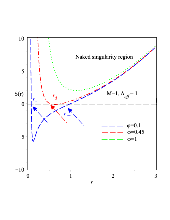
(a)  Behavior of $g_{tt}$

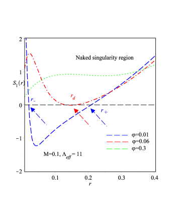
(b)  Behavior of $g_{rr}$

Figure 1: The four-dimensional Maxwell-$f(Q)$ gravity solution’s metric functions, $S(r)$ and $S_{1}(r)$, for different electric charge values $\varphi$, where $\kappa=1$, in the relativistic units. The outer event horizon of the black hole is represented by $r_{+}$, and the inner Cauchy horizon of a black hole by $r_{-}$. Here we put $\gamma=1$.

Similar to this, we can look into the horizons of Eq. (III.2), which can also be found by looking at the solutions of $S_{1}(r)=0$. We show in Fig. 10(a), the behavior of $S_{1}(r)$ that corresponds to the solution (III.2) across different values of the model parameters. Figure 10(a) clearly illustrates the two solutions of $S_{1}(r)$, which match the positions of the outer event horizon $r_{+}$ and inner Cauchy horizon $r_{-}$ of the black hole Brecher et al. (2005). It’s evident that as the electric charge $\varphi$ increases and the mass parameter $M$ decreases, particularly when $\varphi=M$, we move into a parameter space without a horizon. Consequently, the naked singularity replaces the central singularity. This represents an intriguing outcome of the charge of $f(Q)$ gravity. It’s worth noting that our analysis is primarily from a mathematical perspective, and we do not delve into investigating whether such a solution could manifest physically through gravitational collapse. This particular phenomenon is absent in scenarios lacking an electromagnetic sector, as discussed previouslyGonzalez et al. (2012); Capozziello et al. (2013)). Additionally, the two horizons combine and become degenerate for suitable values of $M$ and $\varphi$, resulting in $r_{-}=r_{+}\equiv r_{dg}$. Ultimately, to determine the horizons, we set $S_{1}(r)=0$, thus

$${M_{+}}=r_{+}\left(r_{+}^{2}\Lambda_{eff}+\frac{15\varphi{}^{2}}{8r_{+}^{{2}}}+\frac{45(18\gamma{\varphi}^{5})^{1/3}}{224\sqrt[3]{r_{+}^{10}}}+\frac{9(18\gamma{\varphi}^{5})^{2/3}}{176\sqrt[3]{r_{+}^{14}}}\right).$$ (41)

IV Maxwell-$f(Q)$ gravity with rotating black hole

We conclude this study by deriving solutions for rotating systems that satisfy the field equations within the framework of the polynomial form of $f(Q)$ gravity. To accomplish this, we will depend on the previously extracted static solutions. Specifically, we will apply the subsequent two-parameter rotational transformations as:

$$\bar{\xi}_{i}=-\Omega\leavevmode\nobreak\ {\xi_{i}}+\frac{\sigma_{i}}{l^{2}}\leavevmode\nobreak\ t,\qquad\qquad\qquad\bar{t}=\Omega\leavevmode\nobreak\ t-\sum\limits_{i=1}^{2}\sigma_{i}\leavevmode\nobreak\ \xi_{i},$$ (42)

with $\sigma_{i}$ representing the rotation parameters, and where the static solution’s parameter $\Lambda_{eff}$ is linked to the parameter $l$ by

$$l=-\frac{3}{\Lambda_{eff}}.$$ (43)

Moreover, $\Omega$ is described as

$$\Omega:=\sqrt{1-\sum\limits_{j=1}^{{2}}\frac{\sigma_{j}{}^{2}}{l^{2}}}.$$

Thus, we obtain the following form for the electromagnetic potential (35):

$$\bar{q}(r)=-q(r)\left[\sum\limits_{j=1}^{2}\sigma_{j}d\xi^{\prime}_{j}-\Omega dt^{\prime}\right].$$ (44)

It should be noted that, despite the fact that the transformation (42) maintains certain local spacetime properties, it alters them globally, as demonstrated by Lemos (1995), because it combines compact and noncompact coordinates. The following is the representation of the metric for the transformation (42):

$$ds^{2}=-S(r)\left[\Omega d{\bar{t}}-\sum\limits_{i=1}^{2}\sigma_{i}d{\bar{\xi}}\right]^{2}+\frac{dr^{2}}{S_{1}(r)}+\frac{r^{2}}{l^{2}}\sum\limits_{i=1}^{2}\left[\sigma_{i}d{\bar{t}}-\Omega\,l^{2}d{\bar{\xi}}_{i}\right]^{2}-\frac{r^{2}}{l^{2}}\left(\sigma_{1}d{\bar{\xi}}_{2}-\sigma_{2}d{\bar{\xi}}_{1}\right)^{2},$$ (45)

In this case, $0\leq\xi_{i}<2\pi$, $-\infty<t<\infty$, $0\leq r<\infty$, and $i=1,2$. The static configuration (20) can be recovered as a specific instance of the generic metric stated above when the rotation parameters are set to equal zero. The coordinate transformations (42) can then be inverted to yield the static spacetime (III.2).

We observe that the transformation (42) is locally realizable but not globally, given that the horizon’s closed curves cannot be reduced to zero, the manifold’s first Betti number is one Stachel (1982); Bonnor (1980).

In power-law $f(Q)$ gravity, we have succeeded in extracting the rotating charged AdS black hole solution. This is one of the primary findings of the current work and a novel solution. Regarding the singularity properties, the static solution of (III.2) will exhibit the same characteristics, as we can observe from the structure of (45). As a result, the discussion and all of the findings in subsection III.2 also apply to the previously mentioned rotating solutions. Thus, a singularity appears as $r=0$, and at the neighborhoods of $r$, the invariants are $(K,R_{\mu\nu}R^{\mu\nu})\sim\sqrt[3]{r^{-8}}$ and $(R,Q_{\mu\nu\rho}Q^{\mu\nu\rho},P_{\mu\nu\rho}P^{\mu\nu\rho},Q)\sim\sqrt[3]{r^{-4}}$, unlike the charged solutions found in GR and STEGR theories. Furthermore, the structure of the horizon exhibits qualitative similarities to the discussion presented at III.2. Interestingly, for small enough values of $\varphi$, we witness the emergence of a naked singularity.

V Black hole (III.2) thermodynamics

The definition of the Hawking temperature is Sheykhi (2010); Hendi et al. (2010); Sheykhi et al. (2010):

$$T_{+}=\frac{S^{\prime}(r_{+})}{4\pi},$$ (46)

where $S^{\prime}(r_{+})\neq 0$ is satisfied and the event horizon is situated at $r=r_{+}$. For $f({\mathcal{Q}})$ gravitational theory, the Bekenstein-Hawking entropy is given by Salako et al. (2013); Bamba et al. (2013)

$$\delta(r_{+})=\frac{A}{4}\frac{df({\mathcal{Q}}_{+})}{d{\mathcal{Q}}_{+}}=\frac{A}{4}\frac{df(r_{+})}{dr_{+}}\frac{dr_{+}}{d{\mathcal{Q}}(r_{+})},$$ (47)

where the event horizon’s area is denoted by $A$.

The black hole’s (III.2) entropy is computed using Eq. (47)

$${\delta_{+}}=\pi\,{r_{+}}^{2}\left(1-\frac{4}{3}\,{\varphi}^{4}\left(32\,{r_{+}}^{{\frac{20}{3}}}-135\,\sqrt[3]{18}\sqrt[3]{{\varphi}^{5}\gamma}\varphi\,\gamma\,{r_{+}}^{4/3}+81\,{18}^{2/3}\left({\varphi}^{5}\gamma\right)^{2/3}\gamma+360\,{\varphi}^{2}\gamma\,{r_{+}}^{8/3}\right){r_{+}}^{-4/3}\left(3\,{18}^{2/3}\left({\varphi}^{5}\gamma\right)^{2/3}\right.\right.$$

$$\left.\left.-4\sqrt[3]{18}\sqrt[3]{{\varphi}^{5}\gamma}\varphi{r_{+}}^{4/3}+8{\varphi}^{2}{r_{+}}^{8/3}\right)^{-2}+4/5{\varphi}^{8}\left(32{r_{+}}^{{\frac{20}{3}}}-135\sqrt[3]{18}\sqrt[3]{{\varphi}^{5}\gamma}\varphi\gamma{r_{+}}^{4/3}+81{18}^{2/3}\left({\varphi}^{5}\gamma\right)^{2/3}\gamma+360{\varphi}^{2}\gamma{r_{+}}^{8/3}\right)^{2}\right.$$

$$\left.{r_{+}}^{-8/3}\left(3\,{18}^{2/3}\left({\varphi}^{5}\gamma\right)^{2/3}-4\,\sqrt[3]{18}\sqrt[3]{{\varphi}^{5}\gamma}\varphi\,{r_{+}}^{4/3}+8\,{\varphi}^{2}{r_{+}}^{8/3}\right)^{-4}\right)\,.$$ (48)

Figure 21(a) illustrates the entropy’s behavior, displaying a positive value

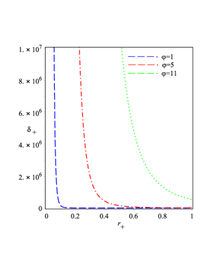
(a)  Heat capacity

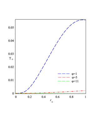
(b)  Hawking’s temperature

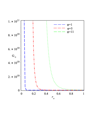
(c)  Gibb’s free energy

Figure 2: (a) The entropy. (b) The Hawking temperature of the black hole solution give by Eq. (III.2). (c) The Gibb’s free energy. Here we put $\gamma=1$

The black hole solution’s (III.2) yields Hawking temperature as:

$${T_{+}}=\frac{1}{4{r}^{11/3}{\pi}}\left(\frac{3}{4}{18}^{2/3}{\varphi}^{4/3}{\gamma}^{2/3}-\sqrt[3]{18}{\varphi}^{2/3}\sqrt[3]{\gamma}{r}^{4/3}+2{r}^{8/3}\right)\left(\Lambda_{eff}r^{2}-{\frac{225}{224}}\sqrt[3]{18}{\varphi}^{8/3}{\gamma}^{1/3}{r}^{-11/3}+{\frac{189}{352}}{18}^{2/3}{\varphi}^{10/3}{\gamma}^{2/3}\right.$$

$$\left.+{\frac{15}{4}}{\varphi}^{2}{r}^{-2}+M\right)\left(\Lambda_{eff}{r}^{2}-{\frac{135}{448}}\sqrt[3]{18}{\varphi}^{8/3}{\gamma}^{1/3}{r}^{-11/3}+{\frac{81}{704}}{18}^{2/3}{\varphi}^{10/3}{\gamma}^{2/3}{r}^{-14/3}+{\frac{15}{8}}{\varphi}^{2}{r}^{-2}+M\right)^{-1},$$ (49)

where the Hawking temperature at the event horizon is denoted by ${T_{+}}$. Figure 21(b), where we plot the Hawking temperature, displays a positive temperature.

Gibb’s free energy, which is the free energy in the grand canonical ensemble, is defined as Zheng and Yang (2018); Kim and Kim (2012):

$$G(r_{h})=M(r_{+})-T(r_{+})\delta(r_{+})$$ (50)

where the temperature, entropy, and quasilocal energy at the event horizon are denoted by the symbols $T(r_{+})$, $\delta(r_{+})$, and $M(r_{+})$. We obtain Gibb’s free energy by applying Eqs. (41), (V), and (V) in (50) as:

$${G_{+}}=-{\frac{1594323}{2560}}\,\left({\frac{16384}{43046721}}\,\gamma\,{r_{+}}^{{\frac{68}{3}}}+{\frac{10240}{129140163}}\,{r_{+}}^{{\frac{74}{3}}}-{\frac{71231488}{40920957}}\,{\gamma}^{3}{r_{+}}^{{\frac{44}{3}}}{\varphi}^{4}-{\frac{133120}{14348907}}\,{r_{+}}^{{\frac{62}{3}}}{\varphi}^{2}\gamma+{\frac{16384}{4782969}}\,{r_{+}}^{{\frac{59}{3}}}M{\gamma}^{2}\right.$$

$$\left.-{\frac{82632800}{10609137}}{r_{+}}^{{\frac{38}{3}}}{\varphi}^{6}{\gamma}^{3}+{\frac{10935}{15488}}{r_{+}}^{2/3}{\varphi}^{12}{\gamma}^{6}-{\frac{48476}{567}}{\varphi}^{8}{\gamma}^{5}{r_{+}}^{{\frac{20}{3}}}+{\frac{5343}{154}}{\varphi}^{10}{\gamma}^{6}{r_{+}}^{8/3}-{\frac{77745}{4312}}{r_{+}}^{14/3}{\varphi}^{10}{\gamma}^{5}+{\frac{3532015}{106722}}{r_{+}}^{{\frac{26}{3}}}{\varphi}^{8}{\gamma}^{4}\right.$$

$$\left.-{\frac{20480{r_{+}}^{{\frac{65}{3}}}M\gamma}{14348907}}-{\frac{204800}{4782969}}{\gamma}^{2}{r_{+}}^{{\frac{56}{3}}}{\varphi}^{2}+{\frac{189}{352}}{18}^{\frac{2}{3}}{\varphi}^{{\frac{34}{3}}}{\gamma}^{{\frac{20}{3}}}+{\frac{17365760}{40920957}}{r_{+}}^{{\frac{50}{3}}}{\varphi}^{4}{\gamma}^{2}+{\frac{7104640}{216513}}{\varphi}^{6}{\gamma}^{4}{r_{+}}^{{\frac{32}{3}}}-\frac{4}{9}{18}^{\frac{2}{3}}{\varphi}^{{\frac{22}{3}}}{\gamma}^{{\frac{17}{3}}}M{r_{+}}^{5}\right.$$

$$\left.+{\varphi}^{8}{\gamma}^{6}M{r_{+}}^{\frac{11}{3}}-{\frac{2080}{243}}{r_{+}}^{{\frac{23}{3}}}M{\gamma}^{5}{\varphi}^{6}+{\frac{208000}{18711}}{r_{+}}^{{\frac{29}{3}}}{\varphi}^{6}{\gamma}^{4}M-{\frac{266240}{531441}}{r_{+}}^{{\frac{47}{3}}}M{\gamma}^{3}{\varphi}^{2}+{\frac{323584}{59049}}{r_{+}}^{{\frac{35}{3}}}M{\gamma}^{4}{\varphi}^{4}\right.$$

$$\left.+{\frac{189440}{1594323}}{r_{+}}^{{\frac{53}{3}}}M{\gamma}^{2}{\varphi}^{2}-{\frac{14113280}{4546773}}{r_{+}}^{{\frac{41}{3}}}M{\gamma}^{3}{\varphi}^{4}-{\frac{835}{308}}{r_{+}}^{{\frac{17}{3}}}{\varphi}^{8}{\gamma}^{5}M+{\frac{46787380}{95482233}}{r_{+}}^{14}{18}^{\frac{2}{3}}{\varphi}^{16/3}{\gamma}^{\frac{8}{3}}-{\frac{19167040}{40920957}}{r_{+}}^{{\frac{46}{3}}}\sqrt[3]{18}{\varphi}^{\frac{14}{3}}{\gamma}^{\frac{7}{3}}\right.$$

$$\left.-{\frac{13059}{2464}}\,\sqrt[3]{18}{\varphi}^{{\frac{32}{3}}}{\gamma}^{{\frac{19}{3}}}{r_{+}}^{4/3}-{\frac{183620}{137781}}\,\left(r_{+}\left({\frac{528520}{302973}}\,r_{+}+M\right){\varphi}^{16/3}+{\frac{42236727}{15552614}}\,{\varphi}^{{\frac{22}{3}}}\right){18}^{2/3}{r_{+}}^{10}{\gamma}^{11/3}-{\frac{20480}{4782969}}\,{18}^{2/3}{r_{+}}^{17}\right.$$

$$\left.\left(\left(-{\frac{8}{15}}\,r_{+}+M\right){r_{+}}^{2}{\gamma}^{5/3}-1/18\,{\gamma}^{2/3}{r_{+}}^{5}-{\frac{24}{5}}{\gamma}^{8/3}M\right){\varphi}^{4/3}+{\frac{7752320}{40920957}}\left(-{\frac{142296}{60565}}{\gamma}^{11/3}M+\left(-{\frac{11266}{109017}}\,{\gamma}^{5/3}{r_{+}}^{3}\right.\right.\right.$$

$$\left.\left.\left.+\left({\frac{38152}{181695}}\,r_{+}+M\right){\gamma}^{8/3}\right){r_{+}}^{2}\right){18}^{2/3}{r_{+}}^{13}{\varphi}^{10/3}-{\frac{5990}{693}}\,{18}^{2/3}\left({\frac{80919}{1686784}}\,{\varphi}^{{\frac{34}{3}}}+{r_{+}}^{2}{\varphi}^{{\frac{28}{3}}}\right){r_{+}}^{2}{\gamma}^{{\frac{17}{3}}}+{\frac{2960}{2187}}\,\left({\varphi}^{16/3}M{r_{+}}^{3}\right.\right.$$

$$\left.\left.+{\frac{32913}{45584}}\,\left({\frac{1850072}{164565}}\,r_{+}+M\right)r_{+}{\varphi}^{{\frac{22}{3}}}+{\frac{43815735}{14039872}}\,{\varphi}^{{\frac{28}{3}}}\right){18}^{2/3}{r_{+}}^{6}{\gamma}^{14/3}-{\frac{16384}{1594323}}\,\left(\left(1/9\,{r_{+}}^{{\frac{64}{3}}}-{\frac{5}{18}}\,{r_{+}}^{{\frac{61}{3}}}M\right){\gamma}^{4/3}\right.\right.$$

$$\left.\left.+{\frac{5}{324}}\,\sqrt[3]{\gamma}{r_{+}}^{{\frac{70}{3}}}+{\gamma}^{7/3}{r_{+}}^{{\frac{55}{3}}}M\right)\sqrt[3]{18}{\varphi}^{2/3}+{\frac{15}{44}}\,\left({\frac{2816}{405}}\,{\varphi}^{{\frac{20}{3}}}{r_{+}}^{{\frac{19}{3}}}M+\left({\frac{50840}{567}}\,{r_{+}}^{16/3}+{r_{+}}^{13/3}M\right){\varphi}^{{\frac{26}{3}}}+{\frac{352137}{34496}}\,{\varphi}^{{\frac{32}{3}}}{r_{+}}^{10/3}\right)\right.$$

$$\left.\sqrt[3]{18}{\gamma}^{16/3}-{\frac{6280}{1701}}\,\left({\frac{17248}{21195}}\,{\varphi}^{14/3}{r_{+}}^{{\frac{31}{3}}}M+\left({\frac{119464}{21195}}\,{r_{+}}^{{\frac{28}{3}}}+{r_{+}}^{{\frac{25}{3}}}M\right){\varphi}^{{\frac{20}{3}}}+{\frac{683763}{193424}}\,{\varphi}^{{\frac{26}{3}}}{r_{+}}^{{\frac{22}{3}}}\right)\sqrt[3]{18}{\gamma}^{13/3}+{\frac{10697920}{4546773}}\,\right.$$

$$\left.\left(\left({\frac{168596}{167155}}\,{r_{+}}^{{\frac{40}{3}}}+{r_{+}}^{{\frac{37}{3}}}M\right){\varphi}^{14/3}+{\frac{26014431}{10296748}}\,{\varphi}^{{\frac{20}{3}}}{r_{+}}^{{\frac{34}{3}}}\right)\sqrt[3]{18}{\gamma}^{10/3}+{\frac{94720}{177147}}\,\left({\gamma}^{10/3}{r_{+}}^{{\frac{43}{3}}}M+{\frac{1135}{41958}}\,{\gamma}^{4/3}{r_{+}}^{{\frac{58}{3}}}\right.\right.$$

$$\left.\left.-{\frac{2725}{9324}}\,{\gamma}^{7/3}\left(-{\frac{304}{2725}}\,{r_{+}}^{{\frac{52}{3}}}+{r_{+}}^{{\frac{49}{3}}}M\right)\right)\sqrt[3]{18}{\varphi}^{8/3}\right){r_{+}}^{-13/3}{\gamma}^{-1}\left(-3/4\,{18}^{2/3}{\varphi}^{4/3}{\gamma}^{2/3}+\sqrt[3]{18}{\varphi}^{2/3}\sqrt[3]{\gamma}{r_{+}}^{4/3}-2\,{r_{+}}^{8/3}\right)^{-4}$$

$$\left(-1/18\,{r_{+}}^{{\frac{20}{3}}}-{\frac{135}{448}}\,\sqrt[3]{18}{\varphi}^{8/3}{\gamma}^{4/3}{r_{+}}^{4/3}+{\frac{81}{704}}\,{18}^{2/3}{\varphi}^{10/3}{\gamma}^{5/3}+{\frac{15}{8}}\,{\varphi}^{2}\gamma\,{r_{+}}^{8/3}+M\gamma\,{r_{+}}^{11/3}\right)^{-1}\,.$$ (51)

Figure 21(c) illustrates the behaviors of the black hole’s Gibb’s free energy (III.2). Gibb’s energy for the black hole solution (III.2) is always positive, indicating that it is more globally stable, as figure 21(c) illustrates.

VI Conclusions

Since the construction of the AdS/CFT procedure, there has been a growing interest in discovering and studying black hole solutions in AdS space. Apart from examining standard gravity, researchers are exploring various modifications of gravity and scenarios involving the Maxwell sector. However, most studies still fall within the realm of modified gravity that alters curvature. In this study, we focus on a static and rotating solution with charge in 4 dimensions within the framework of $f(Q)$ gravitational theory. We emphasize the power-law assumption, which aligns with observations and is considered the most beneficial.

We demonstrate that when the charge is absent, we can derive an AdS solution D’Ambrosio et al. (2022); Nashed (2024). The cosmological constant in this solution is determined by the modifications introduced by $f(Q)$. We analytically derive static solutions with charge, which approach asymptotically AdS when the Maxwell sector is active. The effective cosmological constant varies based on the electric charge and the parameters of the $f(Q)$ modification. This type of solution does not have an uncharged version or a non-metricity (i.e., the linear form of $f(Q)$) or GR limit. It represents a new solution in $f(Q)$ gravity characterized by a power-law behavior, where changes in non-metricity and the inclusion of the Maxwell sector are the primary factors determining its characteristics. Moreover, we demonstrate that the potential $q(r)$ in the solution we found depends on both a higher-order electromagnetic potential and a monopole. This indicates that we could not find a charged solution with just a monopole within the framework of $f(Q)$ gravity.

Next, we investigated the behavior of the singularity of the black hole by deriving various measures of curvature and non-metricity invariants. We discovered that there is a singularity at $r=0$, but its severity is mitigated compared to standard GR due to the structure of $f(Q)$. Furthermore, we analyzed the horizons of the black holes and observed that they have a cosmological horizon as well as the evenan eventizon. However, for sufficiently large electric charges, a naked singularity emerges.

Furthermore, we derived a rotating AdS solution in Maxwell-$f(Q)$ gravity by using the analysis from the static solution and applying suitable changes. The sources of the effective cosmological constant are, as in the static case, the $f(Q)$ and the charged terms. Moreover, in the uncharged case, the singularity and horizon properties remain the same. This solution represents a new type and does not have an uncharged version or a non-metricity counterpart.

Exploring the AdS/CFT correspondence within the framework of non-metricity could greatly benefit from extracting AdS black holes in $f(Q)$ gravity. Comparing this approach to the traditional formulation based on curvature, we anticipate advantages. It would be beneficial if we could derive regular black holes within the $f(Q)$ gravitational theory. This assignment will be addressed in a separate study.

References

- Nester and Yo (1999) J. M. Nester and H.-J. Yo, Chin. J. Phys. 37, 113 (1999), eprint gr-qc/9809049.
- Beltrán Jiménez et al. (2018a) J. Beltrán Jiménez, L. Heisenberg, and T. S. Koivisto, JCAP 08, 039 (2018a), eprint 1803.10185.
- Beltrán Jiménez et al. (2019) J. Beltrán Jiménez, L. Heisenberg, and T. S. Koivisto, Universe 5, 173 (2019), eprint 1903.06830.
- Rünkla and Vilson (2018) M. Rünkla and O. Vilson, Phys. Rev. D 98, 084034 (2018), eprint 1805.12197.
- Beltrán Jiménez et al. (2020) J. Beltrán Jiménez, L. Heisenberg, T. S. Koivisto, and S. Pekar, Phys. Rev. D 101, 103507 (2020), eprint 1906.10027.
- Blixt et al. (2023) D. Blixt, A. Golovnev, M.-J. Guzman, and R. Maksyutov (2023), eprint 2306.09289.
- Beltrán Jiménez and Koivisto (2022) J. Beltrán Jiménez and T. S. Koivisto, Int. J. Geom. Meth. Mod. Phys. 19, 2250108 (2022), eprint 2202.01701.
- Adak (2018) M. Adak, Int. J. Geom. Meth. Mod. Phys. 15, 1850198 (2018), eprint 1809.01385.
- Tomonari and Bahamonde (2023) K. Tomonari and S. Bahamonde (2023), eprint 2308.06469.
- D’Ambrosio et al. (2022) F. D’Ambrosio, S. D. B. Fell, L. Heisenberg, and S. Kuhn, Phys. Rev. D 105, 024042 (2022), eprint 2109.03174.
- Beltrán Jiménez et al. (2018b) J. Beltrán Jiménez, L. Heisenberg, and T. Koivisto, Phys. Rev. D 98, 044048 (2018b), eprint 1710.03116.
- Quiros (2022) I. Quiros, Phys. Rev. D 105, 104060 (2022), eprint 2111.05490.
- Maluf (2013) J. W. Maluf, Annalen Phys. 525, 339 (2013), eprint 1303.3897.
- Aldrovandi and Pereira (2013) R. Aldrovandi and J. G. Pereira, Teleparallel Gravity: An Introduction (Springer, 2013), ISBN 978-94-007-5142-2, 978-94-007-5143-9.
- Cai et al. (2016) Y.-F. Cai, S. Capozziello, M. De Laurentis, and E. N. Saridakis, Rept. Prog. Phys. 79, 106901 (2016), eprint 1511.07586.
- Krššák and Saridakis (2016) M. Krššák and E. N. Saridakis, Class. Quant. Grav. 33, 115009 (2016), eprint 1510.08432.
- Nashed (2018) G. Nashed, Advances in High Energy Physics 2018, 1 (2018).
- Nashed et al. (2019) G. G. L. Nashed, W. El Hanafy, and K. Bamba, JCAP 01, 058 (2019), eprint 1809.02289.
- Nashed and Saridakis (2020) G. G. L. Nashed and E. N. Saridakis, Phys. Rev. D 102, 124072 (2020), eprint 2010.10422.
- Bahamonde et al. (2015) S. Bahamonde, C. G. Böhmer, and M. Wright, Phys. Rev. D 92, 104042 (2015), eprint 1508.05120.
- Bahamonde et al. (2023) S. Bahamonde, K. F. Dialektopoulos, C. Escamilla-Rivera, G. Farrugia, V. Gakis, M. Hendry, M. Hohmann, J. Levi Said, J. Mifsud, and E. Di Valentino, Rept. Prog. Phys. 86, 026901 (2023), eprint 2106.13793.
- Hu et al. (2023) K. Hu, M. Yamakoshi, T. Katsuragawa, S. Nojiri, and T. Qiu, Phys. Rev. D 108, 124030 (2023), eprint 2310.15507.
- Heisenberg (2019) L. Heisenberg, Phys. Rept. 796, 1 (2019), eprint 1807.01725.
- Harko et al. (2018) T. Harko, T. S. Koivisto, F. S. N. Lobo, G. J. Olmo, and D. Rubiera-Garcia, Phys. Rev. D 98, 084043 (2018), eprint 1806.10437.
- Järv et al. (2018) L. Järv, M. Rünkla, M. Saal, and O. Vilson, Phys. Rev. D 97, 124025 (2018), eprint 1802.00492.
- Capozziello et al. (2022) S. Capozziello, V. De Falco, and C. Ferrara, Eur. Phys. J. C 82, 865 (2022), eprint 2208.03011.
- Capozziello et al. (2023) S. Capozziello, V. De Falco, and C. Ferrara, Eur. Phys. J. C 83, 915 (2023), eprint 2307.13280.
- Hu et al. (2024) K. Hu, T. Paul, and T. Qiu, Sci. China Phys. Mech. Astron. 67, 220413 (2024), eprint 2308.00647.
- Qiu et al. (2019) T. Qiu, K. Tian, and S. Bu, Eur. Phys. J. C 79, 261 (2019), eprint 1810.04436.
- Nájera and Fajardo (2022) A. Nájera and A. Fajardo, JCAP 03, 020 (2022), eprint 2111.04205.
- Li and Zhao (2022) M. Li and D. Zhao, Phys. Lett. B 827, 136968 (2022), eprint 2108.01337.
- Khyllep et al. (2021) W. Khyllep, A. Paliathanasis, and J. Dutta, Phys. Rev. D 103, 103521 (2021), eprint 2103.08372.
- Casalino et al. (2021) A. Casalino, B. Sanna, L. Sebastiani, and S. Zerbini, Phys. Rev. D 103, 023514 (2021), eprint 2010.07609.
- Sharma and Sur (2021) M. K. Sharma and S. Sur (2021), eprint 2102.01525.
- Sharma and Sur (2022) M. K. Sharma and S. Sur, Int. J. Mod. Phys. D 31, 2250017 (2022), eprint 2112.08477.
- Sharma and Sur (2023) M. K. Sharma and S. Sur, Phys. Dark Univ. 40, 101192 (2023), eprint 2112.14017.
- Mandal et al. (2020a) S. Mandal, D. Wang, and P. K. Sahoo, Phys. Rev. D 102, 124029 (2020a), eprint 2011.00420.
- Mandal et al. (2020b) S. Mandal, P. K. Sahoo, and J. R. L. Santos, Phys. Rev. D 102, 024057 (2020b), eprint 2008.01563.
- Mandal and Sahoo (2021) S. Mandal and P. K. Sahoo, Phys. Lett. B 823, 136786 (2021), eprint 2111.10511.
- Arora and Sahoo (2022) S. Arora and P. K. Sahoo, Annalen Phys. 534, 2200233 (2022), eprint 2206.05110.
- Gadbail et al. (2022) G. N. Gadbail, S. Mandal, and P. K. Sahoo, Phys. Lett. B 835, 137509 (2022), eprint 2210.09237.
- Paliathanasis (2024) A. Paliathanasis, Phys. Dark Univ. 43, 101388 (2024), eprint 2309.14669.
- Paliathanasis (2023a) A. Paliathanasis, Phys. Dark Univ. 41, 101255 (2023a), eprint 2304.04219.
- Dimakis et al. (2022) N. Dimakis, A. Paliathanasis, M. Roumeliotis, and T. Christodoulakis, Phys. Rev. D 106, 043509 (2022), eprint 2205.04680.
- Paliathanasis (2023b) A. Paliathanasis (2023b), eprint 2310.16357.
- Wang et al. (2022) W. Wang, H. Chen, and T. Katsuragawa, Phys. Rev. D 105, 024060 (2022), eprint 2110.13565.
- Lin and Zhai (2021) R.-H. Lin and X.-H. Zhai, Phys. Rev. D 103, 124001 (2021), [Erratum: Phys.Rev.D 106, 069902 (2022)], eprint 2105.01484.
- Bahamonde et al. (2022) S. Bahamonde, J. Gigante Valcarcel, L. Järv, and J. Lember, JCAP 08, 082 (2022), eprint 2206.02725.
- Calzá and Sebastiani (2023) M. Calzá and L. Sebastiani, Eur. Phys. J. C 83, 247 (2023), eprint 2208.13033.
- Hohmann et al. (2018) M. Hohmann, M. Krššák, C. Pfeifer, and U. Ualikhanova, Phys. Rev. D 98, 124004 (2018), eprint 1807.04580.
- Hohmann et al. (2019) M. Hohmann, C. Pfeifer, J. Levi Said, and U. Ualikhanova, Phys. Rev. D 99, 024009 (2019), eprint 1808.02894.
- Soudi et al. (2019) I. Soudi, G. Farrugia, V. Gakis, J. Levi Said, and E. N. Saridakis, Phys. Rev. D 100, 044008 (2019), eprint 1810.08220.
- Abedi and Capozziello (2018) H. Abedi and S. Capozziello, Eur. Phys. J. C 78, 474 (2018), eprint 1712.05933.
- Hu et al. (2022) K. Hu, T. Katsuragawa, and T. Qiu, Phys. Rev. D 106, 044025 (2022), eprint 2204.12826.
- D’Ambrosio et al. (2023) F. D’Ambrosio, L. Heisenberg, and S. Zentarra, Fortsch. Phys. 71, 2300185 (2023), eprint 2308.02250.
- Heisenberg (2024) L. Heisenberg, Phys. Rept. 1066, 1 (2024), eprint 2309.15958.
- Paliathanasis et al. (2024) A. Paliathanasis, N. Dimakis, and T. Christodoulakis, Phys. Dark Univ. 43, 101410 (2024), eprint 2308.15207.
- Dimakis et al. (2021) N. Dimakis, A. Paliathanasis, and T. Christodoulakis, Class. Quant. Grav. 38, 225003 (2021), eprint 2108.01970.
- Awad et al. (2017) A. M. Awad, S. Capozziello, and G. G. L. Nashed, JHEP 07, 136 (2017), eprint 1706.01773.
- Mandal et al. (2023) S. Mandal, S. Pradhan, P. K. Sahoo, and T. Harko, Eur. Phys. J. C 83, 1141 (2023), eprint 2310.00030.
- Nashed (2023) G. G. L. Nashed (2023), eprint 2312.14451.
- Nashed (2024) G. G. L. Nashed, Symmetry 16 (2024), ISSN 2073-8994, URL https://www.mdpi.com/2073-8994/16/2/219.
- Martinez et al. (2006) C. Martinez, J. P. Staforelli, and R. Troncoso, Phys. Rev. D 74, 044028 (2006), eprint hep-th/0512022.
- Cisterna and Erices (2014) A. Cisterna and C. Erices, Phys. Rev. D 89, 084038 (2014), eprint 1401.4479.
- Bueno and Cano (2016) P. Bueno and P. A. Cano, Phys. Rev. D 94, 124051 (2016), eprint 1610.08019.
- Brecher et al. (2005) D. Brecher, J. He, and M. Rozali, JHEP 04, 004 (2005), eprint hep-th/0410214.
- Gonzalez et al. (2012) P. A. Gonzalez, E. N. Saridakis, and Y. Vasquez, JHEP 07, 053 (2012), eprint 1110.4024.
- Capozziello et al. (2013) S. Capozziello, P. A. Gonzalez, E. N. Saridakis, and Y. Vasquez, JHEP 02, 039 (2013), eprint 1210.1098.
- Lemos (1995) J. P. S. Lemos, Phys. Lett. B 353, 46 (1995), eprint gr-qc/9404041.
- Stachel (1982) J. Stachel, Phys. Rev. D 26, 1281 (1982).
- Bonnor (1980) W. B. Bonnor, J. Math. Phys. 13, 2121 (1980).
- Sheykhi (2010) A. Sheykhi, Eur. Phys. J. C 69, 265 (2010), eprint 1012.0383.
- Hendi et al. (2010) S. H. Hendi, A. Sheykhi, and M. H. Dehghani, Eur. Phys. J. C 70, 703 (2010), eprint 1002.0202.
- Sheykhi et al. (2010) A. Sheykhi, M. H. Dehghani, and S. H. Hendi, Phys. Rev. D 81, 084040 (2010), eprint 0912.4199.
- Salako et al. (2013) I. G. Salako, M. E. Rodrigues, A. V. Kpadonou, M. J. S. Houndjo, and J. Tossa, JCAP 11, 060 (2013), eprint 1307.0730.
- Bamba et al. (2013) K. Bamba, M. Jamil, D. Momeni, and R. Myrzakulov, Astrophys. Space Sci. 344, 259 (2013), eprint 1202.6114.
- Zheng and Yang (2018) Y. Zheng and R.-J. Yang, Eur. Phys. J. C 78, 682 (2018), eprint 1806.09858.
- Kim and Kim (2012) W. Kim and Y. Kim, Phys. Lett. B 718, 687 (2012), eprint 1207.5318.