Neural Honeytrace: A Robust Plug-and-Play Watermarking Framework
against Model Extraction Attacks

Abstract

Developing high-performance deep learning models is resource-intensive, leading model owners to utilize Machine Learning as a Service (MLaaS) platforms instead of publicly releasing their models. However, malicious users may exploit query interfaces to execute model extraction attacks, reconstructing the target model’s functionality locally. While prior research has investigated triggerable watermarking techniques for asserting ownership, existing methods face significant challenges: (1) most approaches require additional training, resulting in high overhead and limited flexibility, and (2) they often fail to account for advanced attackers, leaving them vulnerable to adaptive attacks.

In this paper, we propose Neural Honeytrace, a robust plug-and-play watermarking framework against model extraction attacks. We first formulate a watermark transmission model from an information-theoretic perspective, providing an interpretable account of the principles and limitations of existing triggerable watermarking. Guided by the model, we further introduce: (1) a similarity-based training-free watermarking method for plug-and-play and flexible watermarking, and (2) a distribution-based multi-step watermark information transmission strategy for robust watermarking. Comprehensive experiments on four datasets demonstrate that Neural Honeytrace outperforms previous methods in efficiency and resisting adaptive attacks. Neural Honeytrace reduces the average number of samples required for a worst-case t-Test-based copyright claim from $12,000$ to $200$ with zero training cost. The code is available at https://github.com/NeurHT/NeurHT.

1 Introduction

With the growing scale of training dataset and model parameter, the development of high-performance deep learning models has become increasingly expensive. For example, excluding the labor costs for data collection and processing, training a GPT-3 [4] model on 1,024 NVIDIA Ampere A100 GPUs takes approximately 34 days and incurs a cost of around $500,000. As a result, instead of releasing their models publicly, model owners usually build up Machine Learning as a Service (MLaaS) platforms for paid intelligent services (e.g., ChatGPT , Midjourney ), where users interact with black-box models via a query interface.

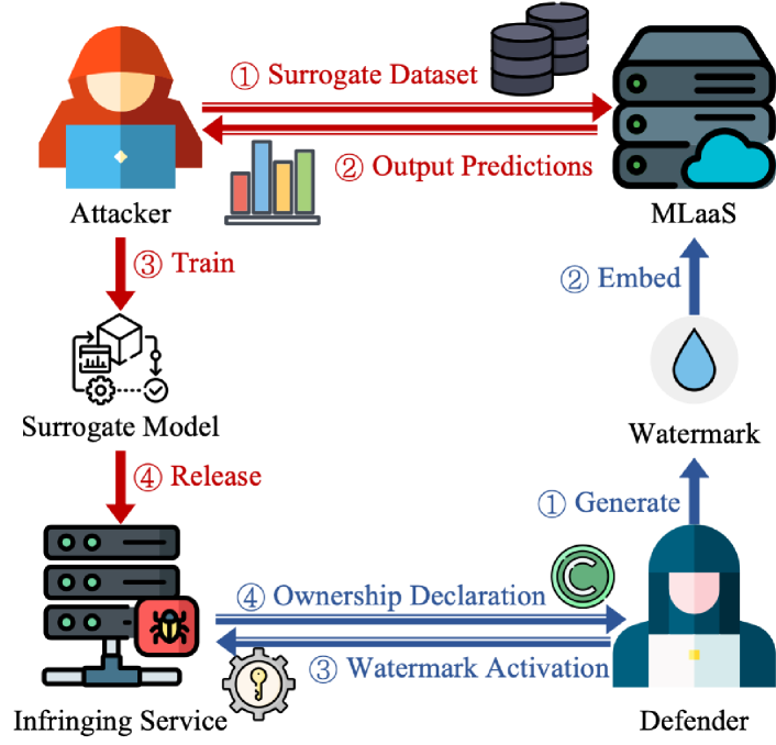
Figure 1: Workflow of MEAs and triggerable watermarking, where red/blue arrows represent attack/defense events.

However, malicious users can still extract valuable information by executing carefully-designed queries to the service interface, enabling them to locally reconstruct the functionality of the victim model with minimal overhead [40, 3, 9, 31, 15, 41], namely model extraction attacks (MEAs). In recent years, model extraction attacks have been extensively studied across various information channels [40, 3], leveraging different data sources [9, 41], and employing diverse learning strategies [13, 6]. Additionally, recent research has also investigated adaptive attacks targeting potential defenses [23, 7, 37]. These mechanisms use effective label recovery strategies to remove misleading perturbations or watermarks embedded in the output predictions, causing severe challenges to the copyright protection of MLaaS applications.

To mitigate the risk of model extraction attacks, a variety of defense mechanisms have been proposed, including model extraction detection [15, 18], prediction perturbation [17, 20, 27, 37], and model watermarking [14, 36, 21, 8, 25]. Compared to the other two passive defenses, model watermarking aims to implant triggerable watermarks into the stolen model, allowing the model owner to assert ownership by activating the watermarks during inference. Recently, backdoor-like watermarks [21, 14, 25] have showed great potential for watermark embedding and capability retention. Fig. 1 provides an overview of the workflow of model extraction attacks and triggerable watermarking methods, where the watermark is embedded in the output predictions and then transmitted to the stolen model.

Despite the success of previous solutions, existing watermarking strategies still face challenges in terms of flexibility and robustness. For example, the watermark embedding process in existing methods [21, 14, 25] requires extensive model retraining. Once embedded, these watermarks cannot be easily removed or modified. Some methods, including the state-of-the-art one, MEA-Defender [25], are designed for soft-label black-box scenarios, resulting in significant performance degradation in hard-label settings—the most common scenario in MLaaS. Moreover, existing approaches are only evaluated against naive attacks, where attackers have no knowledge about potential defenses. As shown in Sec. 5.2, these methods exhibit limited robustness against adaptive model extraction attacks. Tab. 1 compares the capability of different watermarking strategies.

Therefore, we propose Neural Honeytrace, a robust plug-and-play watermarking framework against model extraction attacks. We begin by developing a watermark transmission model from an information-theoretic perspective. Based on this framework, we analyze the embedded watermark information, its transmission, and its robustness in terms of information entropy, channel capacity, and noise resilience. We discovered that triggered watermarks face challenges against adaptive attacks due to the limited channel capacity and additional noises. Building on these insights, we introduced: (1) a training-free watermarking method for plug-and-play and flexible watermarking, and (2) a multi-step watermark information transmission strategy for robust watermarking. The main contributions of this paper are summarized as follows:

1. We propose Neural Honeytrace, the first training-free triggerable watermarking framework. It is designed as a plug-and-play manner, offering the flexibility for seamless removal or modification post-deployment.

2. We establish a watermark transmission model using the information theory, which addresses several open questions pertaining to triggerable watermarking, including the nature of watermarking information and the factors affecting the success rate of watermarking transmission. Guided by the model, we introduce two watermarking strategies which enable training-free watermark embedding and robust transmission.

3. We evaluate Neural Honeytrace against various model extraction attacks, including adaptive attacks with advanced attackers, and empirically show that Neural Honeytrace achieves significant better robustness and less overhead compared to existing methods. Neural Honeytrace reduces the average number of samples required for a worst-case t-Test-based copyright claim from $12,000$ to $200$ with zero training cost.

Table 1: Comparison of watermarking strategies against model extraction attacks.

Method	IP Declaration	No Prior	Training-free & Flexibility	Adaptive Attack
EWE [14]
DAWN [36]
Composite [21]
SSLGuard [8]
MEA-Defender [25]
Neural-HT (Ours)

2 Background

2.1 Model Extraction Attack

The goal of model extraction attacks is to rebuild the functionality of the victim model $\mathcal{F}$ locally. To achieve this object, attackers first collect or synthesize an unlabeled surrogate dataset $\mathbb{D}_{s}=\{{X}_{1},{X}_{2},...,{X}_{n}\}$, and then utilize the victim model $\mathcal{F}$ to label the surrogate dataset $\mathbb{D}_{s}$ and get the corresponding label set $\mathbb{Y}_{s}=\{{Y}_{1},{Y}_{2},...,{Y}_{n}\}$. The type of label ${Y}$ is determined by the setting of MLaaS (e.g., scores, probabilities, and hard-labels). Subsequently, attackers can train a surrogate model $\mathcal{F}_{s}$ following the optimization problem:

$$\underset{\mathcal{F}_{s}}{\operatorname*{arg\,min}}~\underset{({X},{Y})\in(\mathbb{D}_{s},\mathbb{Y}_{s})}{\mathbb{E}}\left[\mathcal{L}\left(\mathcal{F}_{s}\left({X}\right),{Y}\right)\right]$$

where $\mathcal{L}$ is the loss function for evaluating the distance between the outputs of $\mathcal{F}$ and $\mathcal{F}_{s}$. After training, the surrogate model should have similar functionality with the victim model, thus attackers can provide stolen services as shown in Fig. 1.

The basic model extraction attack defined above may fail under perturbation-based defenses [17, 20, 27, 37]. Therefore, attackers introduced more advanced adaptive attacks to bypass potential defenses. Denote the perturbed prediction set as $\hat{\mathbb{Y}}_{s}=\{{Y}_{1}+{P}_{1},{Y}_{2}+{P}_{2},...,{Y}_{n}+{P}_{n}\}$, where ${P}_{i}$ represents the perturbation added on ${Y}_{i}$ by defense strategies. Adaptive model extraction attacks adopt different recovery mechanisms $\mathcal{R}(.)$ to recover $\mathbb{Y}_{s}$ from $\hat{\mathbb{Y}}_{s}$. For example, Smoothing Attack [23] performs several image augmentations on each query image and leverages the average of all predictions of each sample to recover the unperturbed labels.

2.2 Triggerable Watermarking

Triggerable watermarking strategies [21, 14, 8, 25] aim at implanting watermarks that can survive during model extraction attacks into the target model. Similar to backdoor activation in backdoor attacks, model owners can use predefined triggers to activate watermarks in stolen models and utilize special model outputs for ownership declaration. Existing triggerable watermarking methods follow the injection of backdoors, for a predefined watermark trigger ${T}$, the watermarking process can be described as the following optimization problem:

$$\underset{\mathcal{F}_{w}}{\operatorname*{arg\,min}}~\underset{({X},{Y})\in(\mathbb{X},\mathbb{Y})}{\mathbb{E}}\left[\mathcal{L}\left(\mathcal{F}_{w}\left({X}\right),{Y}\right)+\alpha\mathcal{L}\left(\mathcal{F}_{w}\left(\tau({X},{T})\right),\hat{{Y}}\right)\right]$$ (1)

where $\mathcal{F}_{w}$ is the watermarked model, $(\mathbb{X},\mathbb{Y})$ are the sets of training data and corresponding labels, $\alpha$ is the weight parameter which balances the watermarking success rate and clean accuracy, $\tau(.,.)$ represents the watermark injection mechanism, and $\hat{{Y}}$ denotes the special output for IP declaration.

A fundamental challenge for triggerable watermarks is they need to survive during model extraction, where the surrogate dataset may not contain the watermark trigger predefined by defenders. Existing methods introduced different assumptions and addressed this challenge empirically by adding regularization terms to Eq. 1 [14, 8] or designing specialized triggers [21, 25]. However, these solutions often introduce additional computational overhead and are not robust against adaptive model extraction attacks.

2.3 Hypothesis Test

Triggerable watermarking enables defenders to claim ownership of the stolen model using hypothesis test [14]. The sample size $N$ required for ownership claim can be calculated using the following equation:

$$N=\frac{2(Z_{\alpha/2}+Z_{\beta})^{2}}{d^{2}}$$ (2)

where $Z_{\alpha/2}$ is the critical value of the significance level, $Z_{\beta}$ is the power, and $d$ is the effect size. For watermarking scenarios, the effect size $d$ is the watermark success rate (WSR). As depicted in Fig. 2, the number of samples required grows exponentially as the success rate of watermarking decreases.

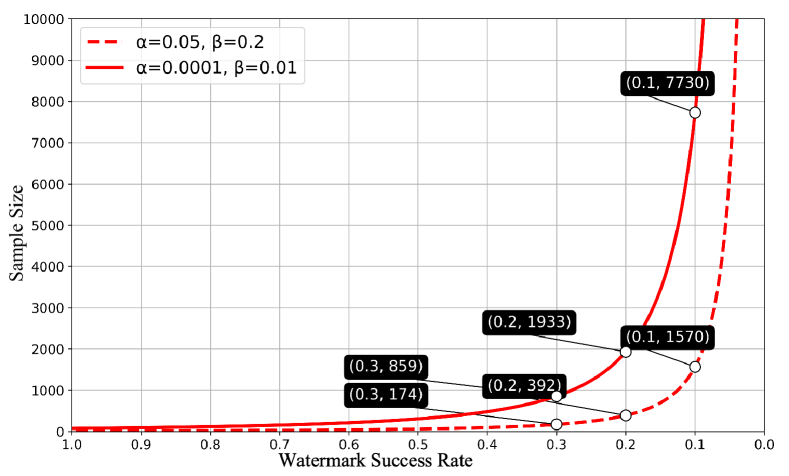
Figure 2: Sample size required for ownership claim.

2.4 Threat Model

Attacker’s goal. As defined in Sec. 2.1, the primary goal of model extraction attackers is to reconstruct the functionality of the victim model locally. We assume the victim model is deployed as a black-box service, which means that attackers can only access output predictions through the interface provided by the model owner.

Attacker’s capability. We consider attackers who lack direct access to the training dataset but possess knowledge of the task domain (e.g., image classification, face recognition etc.) and utilize open-source datasets from the corresponding domains to perform attacks.

To account for varying levels of sophistication, we classify attackers into three categories based on their knowledge of potential defenses: 1) naive attackers who have no prior knowledge, 2) adaptive attackers who know the type of deployed defenses but do not know the implementation details, and 3) oracle attackers who have full knowledge about the deployed defense mechanisms.

Defender’s Capability. We assume that the defender does not have control over the model training process and provides defense services after the target model has been deployed. The defender possesses a watermark dataset along with the corresponding watermark features extracted by the target model. During the watermark embedding process, the defender can modify the predictions of the target model. For watermark activation, the defender interacts with the suspicious model under black-box constraints with limited query numbers.

3 Watermark Transmission Model

Previous studies [14, 21, 8, 25] have empirically tackled challenges associated with triggerable watermarks, such as achieving a high watermark success rate. However, some fundamental questions remain unexplored:

1. Why are watermarks transmitted to stolen models even when they are not explicitly activated?

2. Why do existing methods struggle against adaptive attacks? Specifically, what aspects of watermarking strategies affect the watermark success rate?

The first question explores whether we can interpretably design watermarking methods that operate without relying on additional model training, while the second focuses on identifying strategies to enhance the robustness of watermarking against adaptive extraction attacks.

By examining the watermark transmission process, we identify its primary objective: to transfer specific information from the watermarked model to the stolen model. This process can be modeled as a message transmission problem. Accordingly, we develop a watermark transmission model grounded in information theory to analyze triggerable watermarks.

3.1 Elements

Initially, we modeled the watermark transmission process following the classic message transmission model. As illustrated in Fig. 3, the model owner designs a watermark represented by the message ${W}$. This message is then encoded by an encoder, denoted as $f_{n}$, according to a predefined strategy. The encoded message is transmitted via the model outputs, which serve as the communication channel. If the attacker successfully receives and decodes the watermark message, it becomes embedded in the stolen model.

According to the model, three elements determine the performance of watermark transmission:

Source. The format of watermark message ${W}$ determines the amount of information contained in it, which can be quantified using information entropy:

$$H({W})=-P({W})\texttt{log}\left(P({W})\right)$$

where $P({W})$ is the probability distribution of ${W}$.

Encoding. In watermark transmission scenarios, the encoding process determines how watermarks change model outputs, which can described as:

$$\hat{{O}}={O}~\oplus~f_{n}({W},\mathbb{A})$$

where $\mathbb{A}$ is the alphabet for encoding, $\hat{{O}}$ and ${O}$ denote the modified and the original output, respectively.

Channel. According to Shannon’s theorem [34], the channel capacity $C$ can be calculated using mutual information $I$:

$$C=\underset{P({X})}{\operatorname*{arg\,max}}~I({X},{Y})$$ (3)

For watermark transmission, ${X}$ and ${Y}$ both represent the output probability, thus we have ${X}={Y}={O}$, and $C=H({O})$.

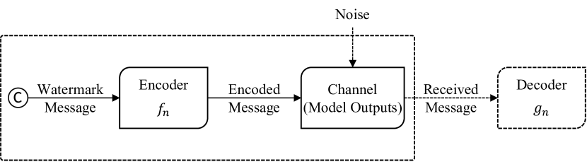
Figure 3: Watermark transmission model.

3.2 Theoretical Analysis

Given the three elements, we can answer the following questions by analyzing the features of these elements in the triggerable watermark transmission scenario.

Figure 4: Watermark information transmitted by EWE [14] on a ResNet-18 model trained on the CIFAR-10 dataset.

1. What is the message generated by the source in the transmission of different watermarks?

For non-triggerable watermarking method DAWN [36], it randomly flips $0.5\%$ of the labels of input samples and utilize these samples as watermarks. Therefore, the watermark message for DAWN is "Does the sample belong to the watermark set?", and $H({W})\approx 0.05$ bit.

However, for triggerable watermarks [14, 21, 8, 25], the source information can not be "Does the sample contain the trigger?" because triggers are not distributed in the surrogate dataset, making $H({W})\approx 0.0$. Instead, we observe that the similarities of input samples and watermark triggers are transmitted. As depicted in Fig. 4, by gradually replacing the corresponding region with the watermark trigger, the probability of the target class gradually increases (gray line). A similar trend can be observed on extraction query examples(blue plots), too. Previous work uses the long-tailed effect of backdoors to characterize this phenomenon [44]. As the result, the stolen model will learn the relationship between trigger similarity and output probability of the target class.

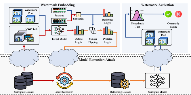
Figure 5: Overview of Neural Honeytrace, where red arrows represent the transmission of attack-related information, blue arrows indicate the transmission of watermark information, and yellow arrows depict the fusion of these two types of information.

2. Why existing triggerable watermarks fail to transmit in adaptive attack scenarios?

Based on the observations in Question 1, we address Question 2 by analyzing and comparing the channel capacity and transmission rate under different model and attack settings. Some adaptive attacks narrows the channel capacity (e.g., Top-1 Attack), while others introduce noise in watermark transmission [13, 23, 7, 37]. Initially, we provide an running example following Fig. 4 to show why existing methods are effective against naive attacks:

We begin by estimating the information entropy of the transmitted similarities. Assuming the similarity distribution follows a normal distribution, $N(\mu,\sigma^{2})$, the information entropy is given by $H({W})=\frac{1}{2}\ln(2\pi e\sigma^{2})$, where $\sigma^{2}=\mathbb{E}[(X-\mu)^{2}]$ is determined by the query data distribution and the similarity calculation method. For instance, in Fig. 4, setting the precision of similarity values to $0.01$ results in an estimated information entropy of $H({W})\approx 4.98$.

In soft-label black-box scenarios, we can estimate the channel capacity using Eq.3. For example, in Fig.4, if the precision of output probabilities is set to $0.01$, the channel capacity is approximately $C\approx 11.74$. By Shannon’s theorem [34], given an acceptable error rate $e$, there exists an encoding strategy that ensures:

$$R(e)=\frac{C}{1-Q(e)}$$ (4)

where $Q(e)=-\left[elog(e)+(1-e)log(1-e)\right]$ and $R(e)$ represents the maximum transmission rate. We observe that if $C\geq R$, there exists a encoding strategies that makes $e\rightarrow 0$, which means the watermark information can be transmitted correctly with close to 100% probability . Furthermore, for a balanced dataset, the label information entropy is approximately $H({L})\approx\texttt{log}N$. In Fig. 4, $H({L})\approx 2.3$ and since $H({L})+H({W})\leq C$, watermark transmission will not compromise the transmission of label information.

However, for Top-1 Attack scenarios [23, 37], the maximum channel capacity satisfies $C_{max}=\texttt{log}N$. In Fig. 4, $C_{max}=\texttt{log}10\approx 2.3$, according to Eq. 4, the error rate $e\rightarrow 1$, which means the channel is not able to transmit watermark information with a high probability. Moreover, even if the value of $N$ becomes large enough for transmitting watermark information, the channel is exclusive, i.e., only one of the watermark or label information can be transmitted through a single query, resulting in failed transmission.

For recover-based adaptive attacks [13, 23, 7, 37], the label recover process can be observed as different channel noises in watermark transmission. For example, Smoothing Attack [23] performs image augmentations on each input for several times and utilizes the average prediction to train the surrogate model. Denote the watermark information (similarity) as $s_{1}$, $k-1$ i.i.d. noises as $(s_{2},s_{3},...,s_{k})\sim N(\mu_{s},\sigma_{s}^{2})$, the error probability can be calculated as:

$$P(|y-s_{1}|>\epsilon)=2\cdot Q\left(\frac{\epsilon-\frac{(k-1)}{k}\cdot(\mu_{s}-s_{1})}{\sqrt{\frac{k-1}{k^{2}}\cdot\sigma_{s}^{2}}}\right)$$ (5)

where $y$ denotes the received watermark information (similarity), $\epsilon$ is the accepted bias threshold, and $Q(\cdot)$ is the tail probability function of the standard normal distribution. We put the detailed derivation of Eq. 5 in Appendix A. According to Eq. 5, larger $\sigma_{s}^{2}$ will lead to higher error probability, which requires more robust watermark encoding strategies.

4 Neural Honeytrace Design

In this section, we introduce our watermarking framework, Neural Honeytrace. We first provide the brief workflow of Neural Honeytrace in Sec. 4.1. Then we provide detailed description of training-free watermark embedding and multi-step watermark transmission in Sec. 4.2 and Sec. 4.3.

4.1 Overview

Different from existing methods which implant watermarks into the target model via retraining or finetuning, Neural Honeytrace aims at implanting triggerable watermarks into the stolen model during model extraction attacks without introducing additional training cost.

Motivated by the watermark transmission model, we have observed that the watermark information transmitted by triggerable watermarking is the similarity of query features and watermark triggers. Therefore, Neural Honeytrace directly embeds the similarity into the predictions. Meanwhile, model extraction attackers may utilize label recover strategies to remove watermark information encoded in the predictions, which can be considered as noises introduced in the channel of watermark transmission. The channel capacity may also be limited in several conditions (e.g., quantized output and hard-label output), making it difficult to transmit the full watermark information in a single query. To address this challenge, Neural Honeytrace utilizes similarity-based label flipping to achieve multi-step watermark transmission, which is robust against different prediction recover strategies and applicable for limited channel capacity.

Fig. 5 provides an overview of the workflow of generic model extraction attacks and Neural Honeytrace. For model extraction attacks, attackers first use an unlabeled surrogate dataset to query the target model through interfaces provided by the model owner. After getting the predictions, attackers may adopt different label recover strategies to erase potential watermark information and reconstruct a retraining dataset using the recovered predictions and original inputs. This dataset is then used to train the surrogate model and reproduce the functionality of the target model locally.

For Neural Honeytrace, the watermarking process consists of four steps. Step 1: defenders initially select watermarks to be transmitted from the watermark pool (e.g., random watermark, semantic watermark, and composite watermark etc.). Step 2: the target model extracts the watermark features and query features respectively and makes predictions on the query samples. Step 3: Neural Honeytrace calculates the similarity of these two features and embeds the similarity into the predictions by mixing the reference logits (target logits of watermarking) and the original logits following the similarity value. Step 4: Neural Honeytrace establishes a probability-guided label-flipping matrix according to the similarity. By encoding similarity values into the prediction distribution of different queries, this matrix enables multi-step watermarking transmission, which is robust against adaptive attacks.

In stolen model detection and ownership claim, defenders use watermarked samples to query the suspicious model and perform a hypothesis test utilizing the predictions. According to Eq. 2, given the watermark success rate (i.e., the ratio that suspicious model makes certain predictions on watermarked samples), if the total number of watermarked samples is lager than the lower bound, then the suspicious model can be considered statistically significant as having a watermark.

4.2 Training-free Watermark Embedding

As we analyzed in Sec. 3.2, the information transmitted by triggerable watermarks is the similarity of query features and watermark features, and the message channel is the output predictions. Therefore, we can directly calculate and encode the similarity into predictions without additional training. So the initial questions become watermark selection, similarity calculation, and similarity embedding.

Watermark generation. The form of watermarks will influence the cost of watermarking process. Previous methods have introduced different watermark generation strategies, e.g., EWE [14] utilized white pixel blocks as triggerable watermarks, while Composite Backdoor [21] and MEA-Defender [25] used spliced in-distribution samples as triggers. According to the information bottleneck theory [39], the training process of neural networks is solving a min-max mutual information problem. For any $i\geq j$ it holds that:

$$I({X};{Y})\geq I({Y};{f}_{j})\geq I({Y};{f}_{i})\geq I({Y};\hat{{Y}})$$

where ${X}$, ${Y}$ are input samples and corresponding labels, $\hat{{Y}}$ is the prediction, and ${f}_{i}$, ${f}_{j}$ denotes the latent features of the i-th layer and the j-th layer, respectively. Intuitively, label-independent information will gradually lost during the forward process of neural networks. And if the watermark only contains out-of-distribution features (e.g., white pixel blocks), it will introduce additional information for the stolen model to learn and make the watermark transmission process harder to converge. Therefore, Neural Honeytrace adopts composite in-distribution samples as watermarks in the default configuration. We also evaluated Neural Honeytrace with different watermark forms in Sec. 5.3.

Similarity calculation. After selecting the watermark forms, Neural Honeytrace calculates the distances between input queries and registered watermarks. This process is also performed in the last latent space following the information bottleneck theory. Specifically, the similarity of input query $X$ and $N$ registered watermarks can be calculated as:

$$s=d-\frac{1}{N}\sum_{i=1}^{N}\left[f_{-1}({X})-f_{-1}({W}_{i})\right]^{2}$$ (6)

where $d$ is a hyperparameter which balances the watermark success rate and model usability, $f_{-1}(.)$ represents the last layer of the target model, and ${W}_{i}$ denotes the i-th watermark. Intuitively, Eq. 6 calculates the average similarity of the input query and registered watermarks.

Additionally, considering that the attackers probably will not have a large amount of in-distribution data for querying the target model, we adopt a simple algorithm to minimize the impact of watermarking on model availability as follows:

$$s=\begin{cases}s^{2},&\text{if }\text{Max}(\text{SoftMax}(\mathcal{F}({X}_{q})))\geq 0.95\\ s,&\text{else wise}\end{cases}$$ (7)

Similarity embedding. Given the similarity, Neural Honeytrace uses logits-mixing to embed the similarity information into the predictions. Denotes the original logits as $l_{ori}$, the reference logits of the target watermark class as $l_{ref}$, then the mixed logits can be calculated as:

$$l_{mix}=(1-s^{\alpha})\cdot l_{ori}+s^{\alpha}\cdot l_{ref}$$ (8)

where $\alpha>1$ establishes a exponentially increasing relationship between the similarity and the activation of watermark targets. By mixing the logits of real samples, Neural Honeytrace reduces the anomaly of the modified logits.

4.3 Multi-step Watermark Transmission

Training-free watermark embedding enables plug-and-play watermarking, however, the message channel is not always ideal. As analyzed in Sec. 3.2, in hard-label black-box scenarios, the channel capacity may not able to effectively transmit watermark information. Also, adaptive attackers may adopt different label recover strategies, which can be considered as noises in watermark transmission. Therefore, we propose the multi-step watermark transmission strategy to enhance the robustness of Neural Honeytrace.

Embedding watermarks in label distribution. Note that a well-trained neural network will establish a mapping from the input distribution to the label distribution, Neural Honeytrace proposes to embed watermark information in the distribution of predictions. Specifically, for a query sample ${X}_{q}$ and the corresponding watermark similarity $s$ calculated using Eq. 6, Neural Honeytrace flips the label by probability according to the following equation:

$$l_{flip}=\begin{cases}l_{flip},&\text{if }\text{Bernoulli}(s^{\beta})=0\\ l_{ref}+\epsilon,&\text{if }\text{Bernoulli}(s^{\beta})=1\end{cases}$$ (9)

where $\beta>1$ is used to balance model availability and watermark success rate, Bernoulli$(.)$ randomly samples with probability to decide whether to flip the label, and $\epsilon$ is a small random value to maintain randomness. Intuitively, for $s\rightarrow 1$, the input sample will be labeled as the target class with a high probability. And by controlling $\beta$, defenders can determine the flipping ratio for samples with $s<1$. Eq. 9 links the predicted labels to the watermark similarities. As a results, Neural Honeytrace transmits watermark information to the label distribution of the surrogate dataset owned by attackers.

Combining training-free watermark embedding and multi-step watermark transmission, Algorithm 1 summarizes the workflow of Neural Honeytrace.

Algorithm 1 Neural Honeytrace

1:INPUT: Query Sample ${X}_{q}$, Model $\mathcal{F}$, In-distribution Dataset $\mathbb{D}$, Source Classes $k,j$, Composite Mask ${M}$, Watermark Target $t$, Weight Parameters $\alpha,\beta$

2:OUTPUT: Flipped Logits $l_{flip}$

3:$\{{X}_{1}^{k},{X}_{2}^{k},\dots,{W}_{n}^{k}\},\{{X}_{1}^{j},{X}_{2}^{j},\dots,{W}_{n}^{j}\}\leftarrow$ Sample($\mathbb{D}$)

4:for index $i=1$ to $n$ do

5:  ${W}_{i}\leftarrow{X}_{i}^{k}\cdot{M}+{X}_{i}^{j}\cdot(1-{M})$ $\triangleright$ Watermark Generation

6:end for

7:for index $i=1$ to $n$ do

8:  $s\leftarrow s+\frac{1}{n}(d-\left[\mathcal{F}^{-1}({X}_{q})-\mathcal{F}^{-1}({W}_{i})\right]^{2})$

9:end for

10:if $\text{Max}(\text{SoftMax}(\mathcal{F}({X}_{q})))\geq 0.95$ then

11:  $s\leftarrow s^{2}$ $\triangleright$ Similarity Calculation

12:end if

13:${X_{t}}\leftarrow$ Sample($\mathbb{D}$)

14:$l_{mix}\leftarrow(1-s^{\alpha})\cdot\mathcal{F}({X}_{q})+s^{\alpha}\cdot\mathcal{F}({X_{t}})$ $\triangleright$ Similarity Embedding

15:$l_{flip}\leftarrow l_{mix}$

16:if $\text{Bernoulli}(s^{\beta})=1$ then

17:  $l_{flip}\leftarrow\mathcal{F}({X_{t}})+\text{Rand}(\epsilon)$ $\triangleright$ Label Flipping

18:end if

19:return $l_{flip}$

Table 2: Watermarking performance of different methods against different attacks on the target model trained on CIFAR-10.

Query Method	Attack Method	DAWN		EWE		Composite Backdoor		MEA-Defender		Neural Honeytrace
		Acc	WSR	Acc	WSR	Acc	WSR	Acc	WSR	Acc	WSR
KnockoffNet	Naive Attack	85.44%	49.11%	88.71%	39.90%	85.47%	43.80%	88.15%	61.80%	83.23%	65.00%
	S4L Attack	83.21%	48.22%	86.49%	9.60%	83.84%	31.20%	86.50%	42.80%	82.14%	71.80%
	Smoothing Attack	85.06%	6.45%	87.47%	2.10%	85.00%	10.80%	87.66%	15.60%	83.78%	68.80%
	D-DAE	85.91%	46.78%	88.13%	27.20%	85.95%	33.20%	87.99%	56.80%	61.08%	77.40%
	p-Bayes Attack	85.61%	49.78%	88.31%	39.60%	85.48%	42.20%	87.87%	59.80%	85.81%	53.20%
	Top-1 Attack	81.09%	49.44%	82.84%	8.90%	80.13%	26.40%	83.16%	40.80%	81.60%	47.80%
JBDA-TR	Naive Attack	81.41%	45.80%	86.58%	25.60%	81.73%	24.40%	85.82%	44.40%	77.23%	53.60%
	D-DAE	80.74%	48.40%	86.11%	33.20%	81.69%	22.20%	85.59%	49.60%	60.90%	62.60%
	p-Bayes Attack	80.54%	46.67%	86.54%	17.50%	80.75%	20.20%	85.11%	33.80%	78.74%	36.60%
	Top-1 Attack	72.99%	47.10%	75.78%	6.70%	73.50%	17.00%	76.33%	11.60%	72.25%	49.20%
Avg / Max Acc $\downarrow$		82.20% / 85.91%		85.70% / 88.71%		82.35% / 85.95%		85.42% / 88.15%		76.68% / 85.81%
Avg / Min WSR $\uparrow$		43.78% /  6.45%		21.03% /  2.10%		27.14% / 10.80%		41.70% / 11.60%		58.60% / 36.60%
Protected Accuracy $\uparrow$		90.74%		90.44%		90.89%		90.12%		91.37%

Table 3: Watermarking performance of different methods against different attacks on the target model trained on CIFAR-100.

Query Method	Attack Method	DAWN		EWE		Composite Backdoor		MEA-Defender		Neural Honeytrace
		Acc	WSR	Acc	WSR	Acc	WSR	Acc	WSR	Acc	WSR
KnockoffNet	Naive Attack	65.30%	46.60%	66.18%	22.00%	65.17%	27.00%	66.69%	38.00%	46.97%	52.40%
	S4L Attack	62.34%	46.10%	63.62%	6.00%	61.70%	19.00%	63.55%	23.00%	46.65%	61.80%
	Smoothing Attack	64.98%	1.97%	65.76%	1.00%	65.04%	17.00%	64.96%	18.00%	51.68%	76.40%
	D-DAE	63.04%	41.10%	65.09%	1.00%	63.17%	15.00%	64.83%	36.00%	43.23%	29.60%
	p-Bayes Attack	65.00%	47.20%	66.76%	21.00%	65.19%	29.00%	62.96%	21.00%	56.66%	32.60%
	Top-1 Attack	56.57%	48.00%	56.70%	0.00%	55.47%	9.00%	56.69%	14.00%	45.46%	76.40%
JBDA-TR	Naive Attack	55.30%	44.80%	63.63%	2.00%	58.93%	7.00%	62.80%	22.00%	40.70%	71.60%
	D-DAE	51.65%	45.10%	57.22%	0.00%	52.10%	13.00%	57.03%	6.00%	29.34%	29.80%
	p-Bayes Attack	55.68%	47.30%	62.18%	3.00%	56.79%	9.00%	61.78%	18.00%	38.93%	65.80%
	Top-1 Attack	43.35%	49.40%	46.46%	0.00%	43.67%	8.00%	46.53%	2.00%	32.51%	59.80%
Avg / Max Acc $\downarrow$		58.32% / 65.30%		61.36% / 66.76%		58.72% / 65.19%		60.78% / 66.69%		43.21% / 56.66%
Avg / Min WSR $\uparrow$		41.76% /  1.97%		5.60% /  0.00%		15.30% /  7.00%		19.80% /  2.00%		55.62% / 29.60%
Protected Accuracy $\uparrow$		74.21%		70.61%		72.27%		70.67%		73.10%

5 Experiments

In this section, we evaluate Neural Honeytrace against different model extractions and compare it with previous watermarking methods. We first introduce the experiment setup in Sec. 5.1. Then we compare the overall performance of different watermarking strategies against adaptive attacks in Sec. 5.2. In Sec. 5.3, we provide ablation study to further analyze Neural Honeytrace.

5.1 Experiment Setup

Datasets. We use four different image classification datasets to train the target model: CIFAR-10 [19], CIFAR-100 [19], Caltech-256 [11], and CUB-200 [43].

We use another two datasets as surrogate datasets used by model extractions attackers, TinyImageNet-200 [29] for querying target models trained on CIFAR-10 and CIFAR-100, ImageNet-1K [10] for querying target models trained on Caltech-256 and CUB-200.

Models. We use two model architectures to train target models: VGG16-BN [35] for CIFAR-10 and CIFAR-100, and ResNet50 [12] for Caltech-256 and CUB-200. Following previous model extraction defenses [32, 37], the same architectures are used for surrogate models.

Metrics. We use three metrics to evaluate the effectiveness of different watermarking methods:

1. Protected Accuracy indicates the accuracy of the protected model on clean samples, i.e., clean accuracy.

2. Extracted Accuracy (Acc) indicates the clean accuracy of the stolen model reconstructed by attackers.

3. Watermark Success Rate (WSR) measures the proportion of successfully activated watermarks. Specifically, it is the ratio of samples with added triggers that are classified into the target classes by the watermarked model but classified into different classes by non-protected models.

Table 4: Watermarking performance of different methods against different attacks on the target model trained on Caltech-256.

Query Method	Attack Method	DAWN		EWE		Composite Backdoor		MEA-Defender		Neural Honeytrace
		Acc	WSR	Acc	WSR	Acc	WSR	Acc	WSR	Acc	WSR
KnockoffNet	Naive Attack	82.33%	43.40%	82.06%	1.60%	79.56%	1.80%	81.81%	41.60%	74.83%	59.60%
	S4L Attack	80.75%	44.00%	80.50%	3.20%	77.92%	0.00%	79.58%	36.60%	75.05%	47.40%
	Smoothing Attack	80.09%	0.87%	80.44%	2.00%	77.28%	0.60%	79.70%	8.20%	72.78%	33.40%
	D-DAE	81.33%	45.50%	80.76%	1.60%	78.15%	1.20%	80.28%	29.60%	74.46%	39.60%
	p-Bayes Attack	82.12%	44.30%	81.98%	1.60%	80.83%	0.20%	77.20%	20.20%	80.23%	22.20%
	Top-1 Attack	72.47%	49.10%	73.31%	3.20%	71.18%	2.20%	71.62%	29.20%	70.09%	38.60%
JBDA-TR	Naive Attack	77.36%	45.54%	78.31%	0.20%	78.95%	7.00%	76.66%	18.40%	61.64%	48.80%
	D-DAE	74.33%	44.56%	75.09%	0.60%	74.05%	4.80%	71.67%	13.20%	69.53%	46.20%
	p-Bayes Attack	78.07%	47.66%	77.22%	0.00%	78.17%	3.60%	76.86%	19.20%	73.91%	20.40%
	Top-1 Attack	60.99%	48.90%	63.14%	1.60%	61.20%	6.40%	59.23%	10.40%	56.81%	45.00%
Avg / Max Acc $\downarrow$		76.98% / 82.33%		77.28% / 82.06%		75.73% / 80.83%		75.46% / 81.81%		70.93% / 80.23%
Avg / Min WSR $\uparrow$		41.38% / 0.87%		1.56% / 0.00%		2.78% / 0.00%		22.66% / 8.20%		40.12% / 20.40%
Protected Accuracy $\uparrow$		83.88%		83.11%		83.19%		82.78%		82.97%

Table 5: Watermarking performance of different methods against different attacks on the target model trained on CUB-200.

Query Method	Attack Method	DAWN		EWE		Composite Backdoor		MEA-Defender		Neural Honeytrace
		Acc	WSR	Acc	WSR	Acc	WSR	Acc	WSR	Acc	WSR
KnockoffNet	Naive Attack	73.62%	45.48%	73.33%	50.40%	73.89%	67.60%	74.08%	69.40%	42.61%	52.80%
	S4L Attack	53.63%	43.51%	67.83%	40.20%	38.38%	0.00%	69.47%	15.60%	42.42%	53.80%
	Smoothing Attack	68.10%	0.24%	68.15%	1.60%	67.73%	0.00%	68.78%	4.00%	50.00%	34.20%
	D-DAE	64.46%	42.72%	60.44%	16.60%	64.50%	19.20%	64.76%	29.20%	52.65%	40.80%
	p-Bayes Attack	74.19%	43.7 %	72.19%	26.60%	73.58%	47.20%	74.01%	65.20%	54.54%	25.60%
	Top-1 Attack	50.61%	48.43%	49.62%	34.80%	50.86%	67.00%	50.91%	97.60%	36.49%	46.40%
JBDA-TR	Naive Attack	61.03%	45.02%	60.74%	24.20%	59.22%	73.60%	62.50%	75.60%	22.71%	56.20%
	D-DAE	47.78%	48.55%	40.83%	8.40%	45.86%	43.20%	48.93%	13.20%	25.83%	47.60%
	p-Bayes Attack	58.99%	47.26%	58.21%	20.80%	56.52%	60.00%	62.19%	73.20%	35.31%	38.40%
	Top-1 Attack	33.19%	43.67%	34.33%	32.00%	34.22%	83.60%	32.86%	92.20%	24.40%	45.40%
Avg / Max Acc $\downarrow$		58.56% / 74.19%		58.57% / 73.33%		56.48% / 73.89%		60.85% / 74.08%		38.70% / 54.54%
Avg / Min WSR $\uparrow$		40.86% / 0.24%		25.56% / 1.60%		46.14% / 0.00%		53.52% / 4.00%		44.12% / 25.60%
Protected Accuracy $\uparrow$		81.95%		82.40%		82.41%		82.67%		80.13%

Model extraction attack methods. We consider two different query strategies, KnockoffNet [31] and JBDA-TR [15], as basic model extraction attack methods. KnockoffNet utilizes natural samples to query the target model and construct surrogate training datasets, while JBDA-TR uses Jacobian-based data augmentation to generate synthetic data and probe the decision boundary of the target model.

Additionally, we consider the following adaptive attack methods on the basis of KnockoffNet and JBDA-TR:

1. Naive Attack: No adaptive attack is performed.

2. S4L Attack [13]: The loss function consists a CE loss and a semi-supervised loss, which helps train the model on both labeled and unlabeled data.

3. Smoothing Attack [23]: Each sample is augmented and fed into the target model $N$ times, and the prediction is computed as the average of $N$ queries. In experiments of this paper, we set $N=3$.

4. D-DAE [7]: Attackers train a defense detection model and a label recover model to detect and bypass potential defenses. In the default configuration, we use recover models trained on different output perturbation methods. For advanced attacks (oracle attack in Sec. 5.3), we train the recover model on different watermarking strategies.

5. p-Bayes Attack [37]: Attackers use independent and neighborhood sampling to perform Bayes-based estimation for original labels.

6. Top-1 Attack: Only hard-labels are used for training surrogate models, which can be also considered as a defense mechanism if defenders only provide hard-labels.

Watermarking strategies. We compare Neural Honeytrace with the following watermarking strategies in experiments:

1. DAWN [36]: Defenders randomly flip the predicted label of a subset of input queries and record these sample-label pairs as watermarks. In the default configuration, we assume that $50\%$ of all queries are executed by benign users and $50\%$ by model extraction attackers.

2. EWE [14]: Defenders utilize the Soft Nearest Neighbor Loss (SNNL) to minimize the distance between watermark features and natural features.

3. Composite Backdoor [21]: Spliced in-distribution samples are used as watermarks (triggers) to increase the watermark success rate.

4. MEA-Defender [25]: Defenders introduce the utility loss, the watermarking loss, and the evasion loss to balance the model availability and watermark success rate.

Figure 6: Sample size required for t-Test of different methods on different models.

5.2 Experimental Results

Overall performance comparison. We begin by comparing Neural Honeytrace with four baseline methods across four different datasets and six model extraction attack strategies. The experimental results for target models trained on CIFAR-10, CIFAR-100, Caltech-256, and CUB-200 are presented in Tab. 2, Tab. 3, Tab. 4, and Tab. 5, respectively. For each defense, we report both the average and maximum extraction accuracy, as well as the average and minimum Watermark Success Rate (WSR). This approach highlights the effectiveness of various watermarking strategies under both optimal and worst-case scenarios, simulating an average attacker and more sophisticated attackers who select the most effective attack methods. We make the following additional observations based on the experiment results:

Existing watermarking methods are sensitive to dataset scale and data complexity. As shown in Tab. 2 and Tab. 3, for smaller datasets and simpler data, existing watermarking methods are effective against Naive Attacks. However, for larger and more complex datasets, as demonstrated in Tab. 4, in four baseline methods, only MEA-Defender maintains acceptable success rates against Naive Attack. This is due to the increased complexity of the data, which leads to an increase in the information entropy of the output prediction. As a result, the watermark transmission process is subject to more channel noise and requires more robust watermark embedding strategies. Intriguingly, sometimes the sensitivity of dataset may also lead to higher watermark success rate. As shown in Tab. 5, the watermark success rate of Composite Backdoor and MEA-Defender against Top-1 Attack is much higher than other methods, while the extraction accuracy decreases significantly. This is because the features of watermarks and query samples are similar in target models protected by these two defenses, resulting in mislabeling a large mount of model extraction queries during attacks.

Existing watermarking methods are vulnerable to adaptive attacks. The experimental results show that five adaptive attack strategies can weaken the watermark to varying degrees. Overall, the Smoothing Attack and Top-1 Attack have the most significant impact on watermark success when KnockoffNet and JBDA-TR are used as query strategies, respectively. For example, in Tab. 2, for KnockoffNet+Smoothing Attack and JBDA-TR+Top-1 Attack, the average WSR of four baseline methods is $8.74\%$ and $20.60\%$, respectively. According to Eq. 2, a decrease in WSR leads to an exponential increase in the sample size required for an ownership claim. Therefore, existing methods are highly likely to fail in detecting stolen models if attackers have prior knowledge of potential defenses and use adaptive attacks.

MEA-Defender outperforms other baseline defenses. Among four baseline methods, although DAWN achieves the highest average WSR across four datasets, it relies on the assumption that model extraction queries occur in a high percentage of all queries. However, in real world scenarios, the proportion of clean queries should be significantly larger than the proportion of extraction queries as the time the model is online grows, in which case the WSR of DAWN will decrease over time. Therefore, it cannot be used as a stable watermarking method. Compared with EWE and Composite Backdoor, MEA-Defender shows higher a average WSR and better robustness against most adaptive attacks. However, the minimum WSR for MEA-Defender indicates that it will still fail under certain adaptive attacks.

Neural Honeytrace outperforms existing defenses. Compared to existing watermarking strategies, Neural Honeytrace achieves better transferability across different datasets. As shown by comparing Tab. 2 and Tab. 3, the watermark success rate of Neural Honeytrace remains stable as the number of output classes increases. For datasets with more complex features, such as those in Tab.4 and Tab.5, Neural Honeytrace maintains its effectiveness, whereas most previous methods suffer from significant performance degradation. Meanwhile, Neural Honeytrace shows better robustness against different adaptive attacks, as reflected in the minimum watermarking success rate. Fig. 6 provides a visualization of the sample sizes required by different watermarking strategies for ownership claim. Considering both the average and worst case scenarios, it can be seen that Neural Honeytrace requires fewer samples for ownership claims compared to previous methods.

Table 6: Neural Honeytrace with different triggers and different query datasets on the target model trained on CIFAR-10.

Query Method	Attack Method	White Pixel Block		Semantic Object		Composite		CIFAR-10		CIFAR-100		TinyImageNet
		Acc	WSR	Acc	WSR	Acc	WSR	Acc	WSR	Acc	WSR	Acc	WSR
	Naive	83.60%	57.20%	78.74%	25.20%	83.23%	65.00%	89.37%	29.20%	83.86%	47.60%	83.23%	65.00%
KnockoffNet	S4L	82.21%	34.10%	78.42%	21.40%	82.14%	71.80%	88.91%	28.80%	83.01%	47.20%	82.14%	71.80%
	Smoothing	83.65%	19.10%	79.58%	20.40%	83.78%	68.80%	88.57%	31.60%	84.13%	49.60%	83.78%	68.80%
	DDAE	64.55%	49.60%	63.43%	24.80%	61.08%	77.40%	89.21%	30.40%	81.92%	57.00%	61.08%	77.40%
	p-Bayes	84.21%	22.40%	79.37%	24.20%	85.81%	53.20%	90.00%	27.80%	84.58%	40.60%	85.81%	53.20%
	Top-1	79.29%	38.60%	74.68%	19.80%	81.60%	47.80%	89.06%	22.20%	79.74%	41.80%	81.60%	47.80%
JBDA-TR	Naive	78.81%	37.40%	66.83%	23.40%	77.23%	53.60%	77.73%	23.60%	75.81%	47.20%	77.23%	53.60%
	DDAE	72.37%	42.60%	52.84%	50.80%	60.90%	62.60%	74.07%	36.80%	75.46%	71.40%	60.90%	62.60%
	p-Bayes	79.24%	32.80%	69.81%	22.60%	78.74%	36.60%	76.26%	29.40%	76.69%	42.60%	78.74%	36.60%
	Top-1	71.99%	44.80%	57.45%	18.20%	72.25%	49.20%	72.33%	32.00%	69.67%	42.80%	72.25%	49.20%
Avg / Max Acc $\downarrow$		77.99% / 84.21%		70.12% / 79.58%		76.68% / 85.81%		83.55% / 90.00%		79.49% / 84.58%		76.68% / 85.81%
Avg / Min WSR $\uparrow$		37.86% / 19.10%		25.08% / 18.20%		58.60% / 36.60%		29.18% / 22.20%		48.78% / 40.60%		58.60% / 36.60%
Protected Accuracy $\uparrow$		91.28%		91.04%		91.37%		91.37%		91.37%		91.37%

Figure 7: Hyperparameter selection on CIFAR-10. Neural Honeytrace with different query sample size, $d$, $\alpha$, and $\beta$.

5.3 Ablation Study

In this section, we comprehensively evaluate the performance of Neural Honeytrace with different defense settings and against different attack settings.

Different Watermark Triggers. We first compare the watermark success rate of Neural Honeytrace using different watermark triggers. As discussed in Sec.4.2, Neural Honeytrace supports the transmission of various watermarks, and the form of these watermarks influences the cost of the watermarking process. In Tab.6, we evaluate three different watermark triggers: white pixel blocks (used in EWE [14]), a semantic object (e.g., a specific copyright logo), and a composite trigger (the default configuration). For the first two trigger types, we adjust the hyperparameters to ensure that the protected model maintains accuracy similar to that of the default configuration.

As shown in Tab.6, the composite trigger achieves the highest average watermark success rate among the three triggers, which aligns with the analysis in Sec.4.2. Compared to the semantic object trigger, white pixel blocks yield a higher average watermark success rate due to their simpler features, making them easier to learn. However, even the semantic object trigger remains robust against various adaptive attacks. Given its interpretable semantics (e.g., the owner’s logo), it could still have potential applications in real-world scenarios.

Different Query Datasets. Depending on the capabilities and prior knowledge, attackers may use different surrogate datasets to query the target model. In Tab.6, we compare the performance of Neural Honeytrace on a target model trained on CIFAR-10 when attackers use CIFAR-10, CIFAR-100, and TinyImageNet as surrogate datasets, respectively. The experimental results show that for out-of-distribution surrogate datasets (CIFAR-100 and TinyImageNet), attackers achieve similar extraction accuracy, and Neural Honeytrace maintains high watermark success rates. However, when using the same training dataset as the surrogate (CIFAR-10), attackers achieve higher extraction accuracy, while the watermark success rate of Neural Honeytrace decreases. This occurs because Eq.7, which is used to detect potential extraction queries, fails in this case. Nevertheless, even in such scenarios, the watermark success rate remains sufficiently high for ownership claims within $1,000$ queries. And in real-world scenarios, it is less possible for attackers to get access to the training dataset of the target model.

Hyperparameters. Subsequently, we evaluate how the hyperparameters will affect the performance of Neural Honeytrace. Specifically, we consider the query sample size $N$ for model extraction attackers, and the three hyperparameters $d,\alpha,\beta$ used in Neural Honeytrace.

As illustrated in the first column in Fig. 7, we perform $6$ different attacks with KnockoffNet and different sample sizes on the target model trained on CIFAR-10. As the sample size increases from $5,000$ to $50,000$, the extraction accuracy of the stolen model slightly increases, because larger sample sizes help attackers gain more information about the feature space of the target model. At the same time, the watermark success rate remains stable under different sample sizes, which indicates that attackers cannot bypass Neural Honeytrace by adjusting the number of queries.

The other columns in Fig. 7 show the effectiveness of the three hyperparameters, $d,\alpha,\beta$, of Neural Honeytrace. These hyperparameters are used to balance the model availability and the watermark success rate. According to Eq. 6, Eq. 8, and Eq. 9, intuitively, larger $d$ and smaller $(\alpha,\beta)$ leads to stronger watermarks but lower protected accuracy, which can also be observed in Fig. 7. Therefore, given a test dataset and the acceptable maximum drop in accuracy, model owners can identify appropriate hyperparameters.

Figure 8: Detection heatmap of BTI [38] on stolen models with/out Neural Honeytrace.

Figure 9: Neural Honeytrace against pruning-based backdoor removal method CLP [51].

Watermark detection and removal. In Sec. 5.2, we evaluate existing watermarking methods against adaptive model extraction attacks. However, previous research [23] suggests that attackers may employ test-time backdoor defense strategies to prevent triggerable watermarks from being activated. Therefore, we additionally evaluated Neural Honeytrace against different backdoor defenses.

For backdoor detection, we use BTI [38], a backdoor model detection method based on trigger inversion. We conduct multiple model extraction attacks on the target model trained on CIFAR-10, obtaining $10$ stolen models with Neural Honeytrace and $10$ models without any defense. We then calculate the average detection heatmap of BTI on these test models. As shown in Fig. 8, the detection heatmaps exhibit similar trends across class pairs, with no anomalous small values (which would suggest potential backdoors) pointing to the target class (class 9) in Neural Honeytrace. This indicates that Neural Honeytrace is robust against trigger-inversion-based backdoor detection.

For backdoor removal, we use CLP [51], a data-free backdoor removal method based on channel Lipschitzness. Specifically, we first perform model extraction attacks on the target model trained on CIFAR-10 and get the stolen model. Then we perform model pruning on the stolen model and record the watermark success rate. As shown in Fig. 9, as the pruning strength increases, the watermark success rate of Neural Honeytrace remains stable. The watermarking success rate does not decrease even if the cleaning accuracy of the stolen model decreases significantly. This indicates that the watermarks injected by Neural Honeytrace are strongly coupled to the original task and are difficult to remove.

Table 7: Watermarking performance of different methods against oracle attacks (D-DAE + ground-truth predictions). Fidelity indicates the similarity between the predictions of the stolen model and the target model.

Method	Naive			Oracle
	Acc	Fidelity	WSR	Acc	Fidelity	WSR
EWE	88.71%	88.18%	39.90%	86.02%	87.95%	4.40%
Composite	85.47%	87.41%	43.80%	85.25%	87.63%	10.40%
MEA-Defender	88.15%	88.63%	61.80%	86.10%	87.95%	10.80%
Neural H/T	83.23%	81.16%	65.00%	64.19%	65.28%	11.80%

Oracle Attack. We also evaluate Neural Honeytrace against a highly capable attacker with full knowledge of the defense mechanism. Specifically, this attacker possesses a set of samples containing both the ground-truth predictions made by the target model and the corresponding modified predictions generated by watermarking strategies. Using these prediction pairs, the attacker trains a label recovery network following the method in [7] and subsequently trains a surrogate model using the recovered predictions.

As shown in Tab.7, the watermark success rate of triggerable watermarking methods decreases significantly under oracle attacks compared to Naive Attack. However, the extraction accuracy and fidelity achieved by oracle attacks against Neural Honeytrace are substantially lower than those against previous methods. Furthermore, compared to perturbation-based defenses[37], Neural Honeytrace demonstrates even lower extraction accuracy and fidelity, indicating that the stolen model fails to accurately reconstruct the functionality of the target model. Therefore, Neural Honeytrace is more robust than existing methods when defending against oracle attacks. More importantly, model owners can easily change the watermarking details since Neural Honeytrace supports plug-and-play implementation, making it more difficult for attackers to access the defense information.

6 Related Work

6.1 Model Extraction Attack

Existing research reveals that machine learning models have different security risks throughout their lifecycle, threatening the availability [46, 49], integrity [50, 26], and confidentiality [2, 5]. Among these malicious attacks, model extraction attacks aim to breach the confidentiality of closed-source models for two goals: (1) rebuilding the functionality of the target model and use it without payment [40], or (2) conducting black-box attacks on the target model via surrogate models [22]. In this paper, we focus on model extraction attacks that attempt to steal functionality.

Naive Attacks. Previous work have explored using different query strategies to perform model extraction attacks. For example, KnockoffNet [31] and ActiveThief [33] select representative natural samples for querying. Subsequent research found that samples close to the decision boundary contain more parameter information, motivating utilizing synthetic (adversarial) samples to perform attacks. In practice, JBDA-TR [15] utilized the feedback of the target model to guide the synthesis process, while FeatureFool [47] used different adversarial attacks to generate query samples. With the development of data-free distillation techniques [48], some methods utilize generative models to generate query samples (e.g., MAZE [16] and MEGEX [28].)

Adaptive Attacks. To mitigate the threat of model extraction attacks, various defense strategies have been proposed, including detection-based defenses [15, 17] and perturbation-based defenses [45]. In response, several adaptive model extraction attacks have been developed to bypass these defenses. The S4L Attack [13] combines cross-entropy loss with a semi-supervised loss to extract more information with a limited number of queries. The Smoothing Attack [23] augments each sample multiple times and averages the predictions to train the model. D-DAE [7] trains both a defense detection model and a label recovery model to detect and bypass potential defenses. The p-Bayes Attack [37] utilizes independent and neighborhood sampling for real label estimation.

6.2 Model Watermarking

White-box watermarking. White-box watermarking methods aim at defending direct model stealing and embed watermark information in parameters or architectures. For example, Uchida et al. [42] and Adi et al. [1] both embed watermarks in the parameter space and utilize embedding matrix and meta classifier to verify watermarks, respectively. However, these methods require a white-box access to the stolen model, making them less practicable.

Black-box watermarking. In black-box conditions, defenders can only query the suspicious model through certain interfaces. Namba et al. [30] use a set of sample-label pairs to embed a backdoor-like watermark in the target model and verify the ownership by activating the backdoor in the stolen model. The subsequent method SSL-WM [24] migrated this method to protect pretrained models by injecting task-agnostic backdoors. Nevertheless, these methods are ineffective against model extraction attacks, because the watermarks fail to transmit from protected models to stolen models.

Szyller et al. [36] proposed a simple watermarking strategy against model extraction attacks by randomly mislabeling some input queries, but it relied on a strong assumption to achieve ownership declaration that malicious queries can not be far fewer than benign queries. Other methods attempted to enhance the success rate of watermark transmission [14, 8, 25]. For example, EWE [14] links watermarking learning to main task learning closely by adding additional regular terms. As a result, the stolen model will effectively inherit the watermark from the protected model while learning the main task. On the basis of EWE, MEA-Defender [25] adopted the composite backdoor [21] as watermarks, further enhancing the success rate of watermark transmission. However, there is still no effective theoretical framework for watermarking against model extraction attacks.

7 Conclusion, Limitations, and Future Work

In this paper, we propose Neural Honeytrace, a robust plug-and-play watermarking framework. We first model watermark transmission problem from the perspective of information theory. Based on the theoretical analysis, we propose two watermarking strategies: training-free watermark embedding and multi-step watermark transmission, to achieve training-free watermarking and enhance the robustness of watermarking. Experimental results show that Neural Honeytrace is significantly more robust against adaptive attacks. It is also more flexible and can be adjusted or removed in time if needed.

Although Neural Honeytrace mostly maintains the availability of the protected model, it will still introduce slight performance decrement on the target model, which poses the need for distinguishing benign and malicious queries. Neural Honeytrace adopts a simple algorithm to detect potential malicious attacks, which will fail when attackers have access to the training dataset of the protected model. In this case, Neural Honeytrace requires a larger sample size for stolen model detection and ownership declaration. One potential solution is to adaptively and dynamically adjust the parameters of Neural Honeytrace for suspicious and trusted users based on their historical behavior.

The most relevant future work is to implement Neural Honeytrace on generative models such as Stable-Diffusion. Although we mainly evaluated Neural Honeytrace on classification tasks following existing methods, our watermark transmission model suggests that the larger output space of generative models may be able to effectively transmit more watermark information in one query.

Appendix A Theoretical Justification of Equation 5

Denote the watermark information as $s_{1}$, noise signals introduced by Smoothing Attack [23] as $s_{2},s_{3},...,s_{k}$. Then the transmitted message signal $y$ and the corresponding noise signal $n$ can be represented by:

$$y=\frac{s_{1}+s_{2}+...+s_{k}}{k},n=\frac{s_{2}+s_{3}+...+s_{k}}{k-1}$$

Define an error as a received signal that deviates from the transmitted signal by more than a certain threshold $\epsilon$, then the error event is:

$$|y-s_{1}|=\left|\frac{s_{1}+s_{2}+...+s_{k}}{k}-s_{1}\right|>\epsilon$$

Let $X=s_{2}+s_{3}+..+s_{k}$ denote the sum of all noises, assume that $s_{2},s_{3},..,s_{k}$ are i.i.d and with mean $\mu_{s}$ and variance $\sigma_{s}^{2}$, according to the central limit theorem, the distribution of $X$ approximately obeys the normal distribution:

$$X\sim N\left((k-1)\cdot\mu_{s},(k-1))\cdot\sigma_{s}^{2}\right)$$

Thus, the distribution of $y-s_{1}$ approximately obeys:

$$y-s_{1}\sim N\left(\frac{(k-1)}{k}\cdot(\mu_{s}-s_{1}),\frac{k-1}{k^{2}}\cdot\sigma_{s}^{2}\right)$$

Therefore, the error probability (i.e., the probability that $|y-s_{1}|>\epsilon$) satisfies:

$$P(|y-s_{1}|>\epsilon)=P(N\left(\frac{(k-1)}{k}\cdot(\mu_{s}-s_{1}),\frac{k-1}{k^{2}}\cdot\sigma_{s}^{2}\right)>\epsilon)$$

Let the standardized z-distribution be:

$$z=\frac{y-s_{1}-\frac{(k-1)}{k}\cdot(\mu_{s}-s_{1})}{\sqrt{\frac{k-1}{k^{2}}\cdot\sigma_{s}^{2}}}$$

Then the error probability satisfies:

$$P(|y-s_{1}|>\epsilon)=2\cdot Q\left(\frac{\epsilon-\frac{(k-1)}{k}\cdot(\mu_{s}-s_{1})}{\sqrt{\frac{k-1}{k^{2}}\cdot\sigma_{s}^{2}}}\right)$$

where $Q(\cdot)$ is the tail probability function of the standard normal distribution and is a monotonically decreasing function.

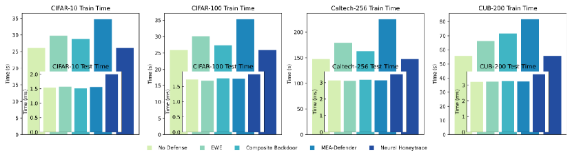
Figure 10: Defense overhead of different triggerable watermarks on different datasets.

Table 8: Neural Honeytrace with different triggers and different query datasets on the target model trained on CIFAR-100.

Query Method	Attack Method	White Pixel Block		Semantic Object		Composite		CIFAR-10		CIFAR-100		TinyImageNet
		Acc	WSR	Acc	WSR	Acc	WSR	Acc	WSR	Acc	WSR	Acc	WSR
	Naive	48.32%	50.20%	51.58%	40.60%	46.97%	52.40%	35.68%	36.20%	66.85%	26.80%	46.97%	52.40%
KnockoffNet	S4L	47.49%	55.80%	51.72%	58.80%	46.65%	61.80%	35.12%	27.60%	66.62%	25.00%	46.65%	61.80%
	Smoothing	54.17%	21.40%	58.59%	23.80%	51.68%	76.40%	47.14%	43.00%	68.24%	22.20%	51.68%	76.40%
	DDAE	42.27%	24.80%	43.34%	23.20%	43.23%	29.60%	40.09%	28.40%	69.30%	16.60%	43.23%	29.60%
	p-Bayes	51.68%	28.60%	52.9 %	30.00%	56.66%	32.60%	47.75%	23.40%	68.08%	20.60%	56.66%	32.60%
	Top-1	45.21%	35.60%	40.91%	29.20%	45.46%	76.40%	33.52%	24.80%	66.64%	26.20%	45.46%	76.40%
JBDA-TR	Naive	33.72%	20.20%	33.08%	11.40%	40.70%	71.60%	20.72%	40.40%	40.06%	20.20%	40.70%	71.60%
	DDAE	40.12%	16.20%	36.46%	10.20%	29.34%	29.80%	23.60%	26.40%	40.72%	14.40%	29.34%	29.80%
	p-Bayes	39.66%	19.40%	40.82%	14.80%	38.93%	65.80%	32.65%	27.80%	41.11%	16.00%	38.93%	65.80%
	Top-1	21.96%	12.80%	21.52%	11.00%	32.51%	59.80%	15.71%	29.20%	33.85%	26.40%	32.51%	59.80%
Avg / Max Acc $\downarrow$		42.46% / 54.17%		43.09% / 58.59%		43.21% / 56.66%		33.20% / 47.75%		56.15% / 69.30%		43.21% / 56.66%
Avg / Min WSR $\uparrow$		28.50% / 12.80%		25.30% / 10.20%		55.62% / 29.60%		30.72% / 23.40%		21.44% / 14.40%		55.62% / 29.60%
Protected Accuracy $\uparrow$		72.40%		72.73%		73.10%		73.10%		73.10%		73.10%

Appendix B Additional Experimental Results

B.1 Overhead of Different Defenses

Fig. 10 compares the defense overhead of different triggerable watermarking methods for protecting target models trained on various datasets. During the training phase, previous triggerable watermarking methods introduce additional time costs due to modifications in the training process. For example, EWE[14] adds regularization terms to the loss function, increasing the time cost of each forward-backward pass. Composite Backdoor [21] and MEA-Defender [25] expand the training dataset with generated data. In contrast, Neural Honeytrace is training-free and can be directly applied to the target model without training.

In the test phase, Neural Honeytrace introduces additional computational overhead for hidden feature hooking and similarity calculation. However, as data complexity increases, the additional overhead introduced by Neural Honeytrace becomes a smaller percentage of the total computational cost, making it cost-acceptable in real-world scenarios.

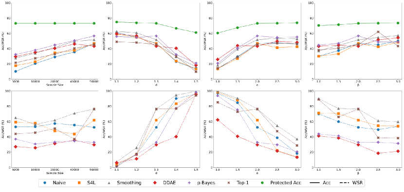
Figure 11: Hyperparameter selection on CIFAR-100. Neural Honeytrace with different query sample size, $d$, $\alpha$, and $\beta$.

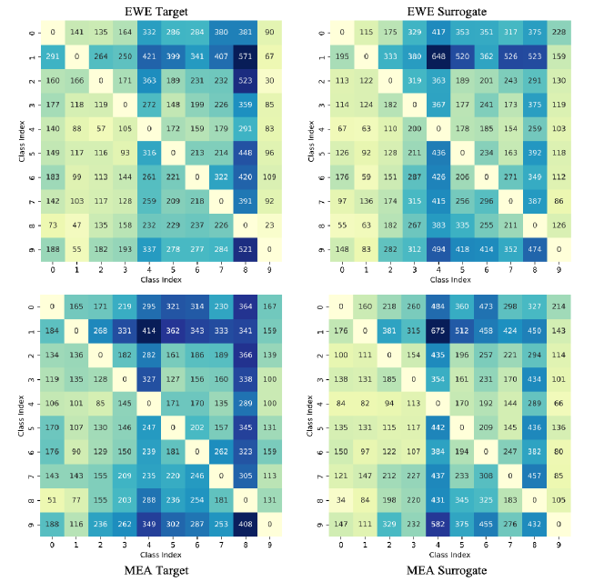
Figure 12: Detection heatmap of BTI [38] on target and stolen models with EWE [14] and MEA-Defender [25].

B.2 Additional Ablation Study

In line with Tab. 6 and Fig. 7, we provide ablation study results on CIFAR-100 in Tab. 8 and Fig. 11.

Different Query Datasets. In Tab.8, we compare the performance of Neural Honeytrace on a target model trained on CIFAR-100 when attackers use CIFAR-10, CIFAR-100, and TinyImageNet as surrogate datasets, respectively. The experimental results show that for out-of-distribution surrogate datasets (CIFAR-10 and TinyImageNet), attackers achieve similar extraction accuracy, and Neural Honeytrace maintains high watermark success rates. However, when using the same training dataset as the surrogate (CIFAR-100), attackers achieve higher extraction accuracy, while the watermark success rate of decreases.

Hyperparameters. We also evaluate the influence of hyperparameters on Neural Honeytrace.

As illustrated in the first column in Fig. 11, we perform $6$ different attacks with KnockoffNet and different sample sizes on the target model trained on CIFAR-100. As the sample size increases from $5,000$ to $50,000$, the extraction accuracy of the stolen model slightly increases, because larger sample sizes help attackers gain more information about the feature space of the target model. At the same time, the watermark success rate remains stable under different sample sizes, which indicates that attackers cannot bypass Neural Honeytrace by adjusting the number of queries.

The other columns in Fig. 11 show the effectiveness of the three hyperparameters, $d,\alpha,\beta$, of Neural Honeytrace. These hyperparameters are used to balance the model availability and the watermark success rate. According to Eq. 6, Eq. 8, and Eq. 9, intuitively, larger $d$ and smaller $(\alpha,\beta)$ leads to stronger watermarks but lower protected accuracy, which can also be observed in Fig. 11. Therefore, given a test dataset and the acceptable maximum drop in accuracy, model owners can identify appropriate hyperparameters.

Test-time Backdoor Detection. Fig.12 presents additional results evaluating existing watermarking strategies against the test-time backdoor detection method BTI[38]. As depicted, BTI fails to effectively detect watermarks embedded in surrogate models for several reasons: (1) For EWE, the watermark success rate is significantly lower compared to conventional backdoor attacks, making it challenging to search for triggers. (2) For MEA-Defender, the composite trigger’s size is large, whereas most existing backdoor detection methods primarily focus on identifying smaller triggers.

Appendix C Implementation Details

Our experiments are conducted on a server with two NVIDIA RTX-4090 GPUs and six Intel(R) Xeon(R) Silver 4210R CPUs. The main software versions include CUDA 12.0, Python 3.9.5, PyTorch 2.0.1, etc.

C.1 Baseline Attacks

Query Strategies. We consider two query strategies for both naive attacks and adaptive attacks:

1. KnockoffNet [31]: Following Tang et al. [37], we utilize KnockoffNet with a random strategy. The attacker randomly chooses $N$ samples from the surrogate dataset and gets the predictions of these samples by querying the target model. Subsequently, the attacker uses the sample-prediction pairs to train the surrogate model locally. In this paper, we set $N=50,000$ for all four dataset.

2. JBDA-TR [15]: JBDA-TR uses generated synthetic samples to test the decision boundaries of the target model. Specifically, JBDA-TR utilizes a small set of samples to query the target model and train a surrogate model locally (similar to KnockoffNet). In this paper, we set the initial size as $10,000$ for better performances. Subsequently, JBDA-TR performs adversarial attacks on the current query dataset and the current surrogate model following:

$$\hat{{X}}_{t}=\hat{{X}}_{t-1}+\mu\cdot\mathrm{sign}\left(\Delta\mathcal{F}(\hat{{X}}_{t-1},\hat{{Y}})\right),~t=1,2,...,T$$

where $\mu$ is the step size, $\hat{{Y}}$ is a randomly selected target, and $T$ is the number of total attack steps. In this paper, we set $\mu=0.01$, $T=8$. JBDA-TR uses these new samples to query the target model and train the surrogate model until the total number of queries reaches $50,000$

Adaptive Attacks. Besides Naive Attack which directly uses predictions of the target model to train the surrogate model, we consider some adaptive attacks:

1. S4L Attack [13]: The training loss function consists a CE loss and a semi-supervised loss, which helps train the model on both labeled and unlabeled data. The semi-supervised loss can be calculated as follows:

$$L_{R}({X},\mathcal{F}_{\theta})=\frac{1}{4N}\sum_{i=0}^{N}\sum_{j=1}^{K}H\left(\mathcal{F}_{\theta}\left(R_{j}({X}_{i}),j\right)\right)$$

where $R(\cdot)$ rotates the input sample by $j\times 90$ degrees, and $H(\cdot)$ calculates the CE loss.

2. Smoothing Attack [23]: Each sample is augmented and fed into the target model $N$ times, and the prediction is computed as the average of $N$ queries. In this paper, we set $N=3$ for all experiments with Smoothing Attack.

3. D-DAE [7]: Attackers train a defense detection model and a label recover model to detect and bypass potential defenses. In the default configuration, we use recover models trained on different output perturbation methods following [37]. For advanced attacks (oracle attack in Sec. 5.3), we train the recover model on different watermarking strategies. Specifically, D-DAE trains a 3-layer neural network to remove perturbations added by defenders, and the training dataset contains $1,000,000$ samples generated from $20$ small shadow models trained on public datasets.

4. p-Bayes Attack [37]: Attackers use independent and neighborhood sampling to perform Bayes-based estimation for original labels. The attacker builds a look-up table:

$$\mathbb{T}=\{(y,p(y)):\exists x\in\mathbb{R}^{d},\exists w,\mathcal{F}_{\theta}(x;w)=y\}$$

when given the perturbed prediction $\hat{y}$, the attacker finds all the $y$ that satisfy $p(y)=\hat{y}$ in the table, then the mean of these Y will be used as the recovered prediction.

C.2 Baseline Defenses

We provide more detailed descriptions about two baseline triggerable watermarking strategies:

1. EWE [14]: Defenders utilize the Soft Nearest Neighbor Loss (SNNL) to minimize the distance between watermark features and natural features. The SNNL can be calculated as:

$$SNNL({X},{Y},T)=-\frac{1}{N}\sum_{i=1}^{N}\mathrm{log}\left\{\frac{\underset{j\neq i,y_{i}=y_{j}}{\sum_{j=1}^{N}}e^{-\frac{{||x_{i}-x_{j}||}^{2}}{T}}}{\underset{k\neq i}{\sum_{k=1}^{N}}e^{-\frac{{||x_{i}-x_{k}||}^{2}}{T}}}\right\}$$

where $T$ is the temperature parameter for controlling the emphasis on smaller distances.

2. MEA-Defender [25]: Defenders introduce the utility loss, the watermarking loss, and the evasion loss to balance the model availability and watermark success rate. The training loss function can be represented as:

$$L =~\beta_{1}\cdot(\underset{x_{wm\in\mathbb{D}_{wm}}}{KL}(f(x_{wm}),x_{i})+\underset{x_{wm\in\mathbb{D}_{wm}}}{KL}(f(x_{wm}),x_{j}))$$

$$+~\beta_{2}\cdot\underset{x_{wm\in\mathbb{D}_{wm}}}{CE}(f(x_{wm}),y_{t}))$$

where the first term is similar to SNNL in EWE, and the second term guarantees the watermarking function.

C.3 Parameters

Hyperparameters for training target and surrogate models. Following [37], we use models trained on ImageNet [10] to initialize the target model. Tab. 9 and Tab. 10 list the hyperparameters used while training target and surrogate models.

Table 9: Hyperparameters for training target models.

Dataset	Model	Epoch	Optimizer	LR / Step / Momentum	Batch Size
CIFAR-10	VGG16-BN	100	SGD	0.01/10/0.5	64
CIFAR-100	VGG16-BN	100	SGD	0.01/10/0.5	64
Caltech-256	ResNet50	100	SGD	0.01/10/0.5	64
CUB-200	ResNet50	100	SGD	0.01/10/0.5	64

Table 10: Hyperparameters for training surrogate models.

Dataset - Query Dataset	Epoch	Optimizer	LR / Step / Momentum	Batch Size
CIFAR-10-TinyImageNet200	30	SGD	0.1/10/0.5	128
CIFAR-100-TinyImageNet200	30	SGD	0.1/10/0.5	128
Caltech-256-ImageNet1000	30	SGD	0.01/10/0.5	32
CUB-200-ImageNet1000	30	SGD	0.01/10/0.5	32

Hyperparameters of Neural Honeytrace on different datasets. Tab. 11 lists the hyperparameters of Neural Honeytrace when watermarking different models trained on different target datasets.

Table 11: Hyperparameters of Neural Honeytrace.

Dataset	Model	Distance $d$	Mixing Power $\alpha$	Flipping Power $\beta$
CIFAR-10	VGG16-BN	0.85	2.0	3.0
CIFAR-100	VGG16-BN	1.00	2.0	3.0
Caltech-256	ResNet50	1.05	2.0	3.0
CUB-200	ResNet50	1.05	2.0	3.0

References

- [1] Yossi Adi, Carsten Baum, Moustapha Cissé, Benny Pinkas, and Joseph Keshet. Turning your weakness into a strength: Watermarking deep neural networks by backdooring. In 27th USENIX Security Symposium, USENIX Security, 2018.
- [2] Shengwei An, Guanhong Tao, Qiuling Xu, Yingqi Liu, Guangyu Shen, Yuan Yao, Jingwei Xu, and Xiangyu Zhang. Mirror: Model inversion for deep learning network with high fidelity. In Proceedings of the 29th Network and Distributed System Security Symposium, NDSS, 2022.
- [3] Lejla Batina, Shivam Bhasin, Dirmanto Jap, and Stjepan Picek. CSI neural network: Using side-channels to recover your artificial neural network information. CoRR, abs/1810.09076, 2018.
- [4] Tom B. Brown, Benjamin Mann, Nick Ryder, Melanie Subbiah, Jared Kaplan, Prafulla Dhariwal, Arvind Neelakantan, Pranav Shyam, Girish Sastry, Amanda Askell, Sandhini Agarwal, Ariel Herbert-Voss, Gretchen Krueger, Tom Henighan, Rewon Child, Aditya Ramesh, Daniel M. Ziegler, Jeffrey Wu, Clemens Winter, Christopher Hesse, Mark Chen, Eric Sigler, Mateusz Litwin, Scott Gray, Benjamin Chess, Jack Clark, Christopher Berner, Sam McCandlish, Alec Radford, Ilya Sutskever, and Dario Amodei. Language models are few-shot learners. In Annual Conference on Neural Information Processing Systems 2020, NeurIPS, 2020.
- [5] Nicholas Carlini, Jamie Hayes, Milad Nasr, Matthew Jagielski, Vikash Sehwag, Florian Tramèr, Borja Balle, Daphne Ippolito, and Eric Wallace. Extracting training data from diffusion models. In 32nd USENIX Security Symposium, USENIX Security, 2023.
- [6] Varun Chandrasekaran, Kamalika Chaudhuri, Irene Giacomelli, Somesh Jha, and Songbai Yan. Exploring connections between active learning and model extraction. In 29th USENIX Security Symposium, USENIX Security, 2020.
- [7] Yanjiao Chen, Rui Guan, Xueluan Gong, Jianshuo Dong, and Meng Xue. D-DAE: defense-penetrating model extraction attacks. In 44th IEEE Symposium on Security and Privacy, S&P, 2023.
- [8] Tianshuo Cong, Xinlei He, and Yang Zhang. Sslguard: A watermarking scheme for self-supervised learning pre-trained encoders. In Proceedings of the 2022 ACM SIGSAC Conference on Computer and Communications Security, CCS, 2022.
- [9] Jacson Rodrigues Correia da Silva, Rodrigo Ferreira Berriel, Claudine Badue, Alberto Ferreira de Souza, and Thiago Oliveira-Santos. Copycat CNN: stealing knowledge by persuading confession with random non-labeled data. In 2018 International Joint Conference on Neural Networks, IJCNN, 2018.
- [10] Jia Deng, Wei Dong, Richard Socher, Li-Jia Li, Kai Li, and Li Fei-Fei. Imagenet: A large-scale hierarchical image database. In 2009 IEEE Computer Society Conference on Computer Vision and Pattern Recognition CVPR, 2009.
- [11] Gregory Griffin, Alex Holub, Pietro Perona, et al. Caltech-256 object category dataset. Technical report, Technical Report 7694, California Institute of Technology Pasadena, 2007.
- [12] Kaiming He, Xiangyu Zhang, Shaoqing Ren, and Jian Sun. Deep residual learning for image recognition. In 2016 IEEE Conference on Computer Vision and Pattern Recognition, CVPR, 2016.
- [13] Matthew Jagielski, Nicholas Carlini, David Berthelot, Alex Kurakin, and Nicolas Papernot. High accuracy and high fidelity extraction of neural networks. In 29th USENIX Security Symposium, USENIX Security, 2020.
- [14] Hengrui Jia, Christopher A. Choquette-Choo, Varun Chandrasekaran, and Nicolas Papernot. Entangled watermarks as a defense against model extraction. In 30th USENIX Security Symposium, USENIX Security, 2021.
- [15] Mika Juuti, Sebastian Szyller, Samuel Marchal, and N. Asokan. PRADA: protecting against DNN model stealing attacks. In IEEE European Symposium on Security and Privacy, EuroS&P, 2019.
- [16] Sanjay Kariyappa, Atul Prakash, and Moinuddin K. Qureshi. MAZE: data-free model stealing attack using zeroth-order gradient estimation. In IEEE Conference on Computer Vision and Pattern Recognition, CVPR, 2021.
- [17] Sanjay Kariyappa and Moinuddin K. Qureshi. Defending against model stealing attacks with adaptive misinformation. In 2020 IEEE/CVF Conference on Computer Vision and Pattern Recognition, CVPR, 2020.
- [18] Manish Kesarwani, Bhaskar Mukhoty, Vijay Arya, and Sameep Mehta. Model extraction warning in mlaas paradigm. In Proceedings of the 34th Annual Computer Security Applications Conference, ACSAC, 2018.
- [19] Alex Krizhevsky, Geoffrey Hinton, et al. Learning multiple layers of features from tiny images. 2009.
- [20] Taesung Lee, Benjamin Edwards, Ian M. Molloy, and Dong Su. Defending against neural network model stealing attacks using deceptive perturbations. In 2019 IEEE Security and Privacy Workshops, S&P Workshops, 2019.
- [21] Junyu Lin, Lei Xu, Yingqi Liu, and Xiangyu Zhang. Composite backdoor attack for deep neural network by mixing existing benign features. In CCS ’20: 2020 ACM SIGSAC Conference on Computer and Communications Security, 2020.
- [22] Yiyong Liu, Zhengyu Zhao, Michael Backes, and Yang Zhang. Membership inference attacks by exploiting loss trajectory. In Proceedings of the 2022 ACM SIGSAC Conference on Computer and Communications Security, CCS, 2022.
- [23] Nils Lukas, Edward Jiang, Xinda Li, and Florian Kerschbaum. Sok: How robust is image classification deep neural network watermarking? In 43rd IEEE Symposium on Security and Privacy, S&P, 2022.
- [24] Peizhuo Lv, Pan Li, Shenchen Zhu, Shengzhi Zhang, Kai Chen, Ruigang Liang, Chang Yue, Fan Xiang, Yuling Cai, Hualong Ma, Yingjun Zhang, and Guozhu Meng. SSL-WM: A black-box watermarking approach for encoders pre-trained by self-supervised learning. In 31st Annual Network and Distributed System Security Symposium, NDSS, 2024.
- [25] Peizhuo Lv, Hualong Ma, Kai Chen, Jiachen Zhou, Shengzhi Zhang, Ruigang Liang, Shenchen Zhu, Pan Li, and Yingjun Zhang. Mea-defender: A robust watermark against model extraction attack. In IEEE Symposium on Security and Privacy, S&P, 2024.
- [26] Hua Ma, Shang Wang, Yansong Gao, Zhi Zhang, Huming Qiu, Minhui Xue, Alsharif Abuadbba, Anmin Fu, Surya Nepal, and Derek Abbott. Watch out! simple horizontal class backdoor can trivially evade defense. In Proceedings of the 2024 on ACM SIGSAC Conference on Computer and Communications Security, CCS, 2024.
- [27] Mantas Mazeika, Bo Li, and David A. Forsyth. How to steer your adversary: Targeted and efficient model stealing defenses with gradient redirection. In International Conference on Machine Learning, ICML, 2022.
- [28] Takayuki Miura, Toshiki Shibahara, and Naoto Yanai. MEGEX: data-free model extraction attack against gradient-based explainable AI. In Proceedings of the 2nd ACM Workshop on Secure and Trustworthy Deep Learning Systems, 2024.
- [29] Mohammed Ali Mnmoustafa. Tiny imagenet. URL https://kaggle. com/competitions/tiny-imagenet, 2017.
- [30] Ryota Namba and Jun Sakuma. Robust watermarking of neural network with exponential weighting. In Proceedings of the 2019 ACM Asia Conference on Computer and Communications Security, AsiaCCS, 2019.
- [31] Tribhuvanesh Orekondy, Bernt Schiele, and Mario Fritz. Knockoff nets: Stealing functionality of black-box models. In IEEE Conference on Computer Vision and Pattern Recognition, CVPR, 2019.
- [32] Tribhuvanesh Orekondy, Bernt Schiele, and Mario Fritz. Prediction poisoning: Towards defenses against DNN model stealing attacks. In 8th International Conference on Learning Representations, ICLR, 2020.
- [33] Soham Pal, Yash Gupta, Aditya Shukla, Aditya Kanade, Shirish K. Shevade, and Vinod Ganapathy. Activethief: Model extraction using active learning and unannotated public data. In The Thirty-Fourth AAAI Conference on Artificial Intelligence, AAAI, 2020.
- [34] Claude Elwood Shannon. A mathematical theory of communication. The Bell system technical journal, 1948.
- [35] Karen Simonyan and Andrew Zisserman. Very deep convolutional networks for large-scale image recognition. In 3rd International Conference on Learning Representations, ICLR, 2015.
- [36] Sebastian Szyller, Buse Gul Atli, Samuel Marchal, and N. Asokan. DAWN: dynamic adversarial watermarking of neural networks. In MM ’21: ACM Multimedia Conference, 2021.
- [37] Minxue Tang, Anna Dai, Louis DiValentin, Aolin Ding, Amin Hass, Neil Zhenqiang Gong, Yiran Chen, and Hai (Helen) Li. Modelguard: Information-theoretic defense against model extraction attacks. In 33rd USENIX Security Symposium, USENIX Security, 2024.
- [38] Guanhong Tao, Guangyu Shen, Yingqi Liu, Shengwei An, Qiuling Xu, Shiqing Ma, Pan Li, and Xiangyu Zhang. Better trigger inversion optimization in backdoor scanning. In IEEE/CVF Conference on Computer Vision and Pattern Recognition, CVPR, 2022.
- [39] Naftali Tishby and Noga Zaslavsky. Deep learning and the information bottleneck principle. In 2015 IEEE Information Theory Workshop, ITW, 2015.
- [40] Florian Tramèr, Fan Zhang, Ari Juels, Michael K. Reiter, and Thomas Ristenpart. Stealing machine learning models via prediction apis. In 25th USENIX Security Symposium, USENIX Security, 2016.
- [41] Jean-Baptiste Truong, Pratyush Maini, Robert J. Walls, and Nicolas Papernot. Data-free model extraction. In IEEE Conference on Computer Vision and Pattern Recognition, CVPR, 2021.
- [42] Yusuke Uchida, Yuki Nagai, Shigeyuki Sakazawa, and Shin’ichi Satoh. Embedding watermarks into deep neural networks. In Proceedings of the 2017 ACM on International Conference on Multimedia Retrieval, ICMR, 2017.
- [43] Catherine Wah, Steve Branson, Peter Welinder, Pietro Perona, and Serge Belongie. The caltech-ucsd birds-200-2011 dataset. 2011.
- [44] Yixiao Xu, Binxing Fang, Mohan Li, Keke Tang, and Zhihong Tian. Lt-defense: Searching-free backdoor defense via exploiting the long-tailed effect. In The Thirty-eighth Annual Conference on Neural Information Processing Systems, NeurIPS, 2024.
- [45] Haonan Yan, Xiaoguang Li, Hui Li, Jiamin Li, Wenhai Sun, and Fenghua Li. Monitoring-based differential privacy mechanism against query flooding-based model extraction attack. IEEE Trans. Dependable Secur. Comput. TDSC, 2022.
- [46] Ziqing Yang, Xinlei He, Zheng Li, Michael Backes, Mathias Humbert, Pascal Berrang, and Yang Zhang. Data poisoning attacks against multimodal encoders. In International Conference on Machine Learning, ICML, 2023.
- [47] Honggang Yu, Kaichen Yang, Teng Zhang, Yun-Yun Tsai, Tsung-Yi Ho, and Yier Jin. Cloudleak: Large-scale deep learning models stealing through adversarial examples. In 27th Annual Network and Distributed System Security Symposium, NDSS, 2020.
- [48] Shikang Yu, Jiachen Chen, Hu Han, and Shuqiang Jiang. Data-free knowledge distillation via feature exchange and activation region constraint. In IEEE/CVF Conference on Computer Vision and Pattern Recognition, CVPR, 2023.
- [49] Zhiyuan Yu, Yuanhaur Chang, Ning Zhang, and Chaowei Xiao. SMACK: semantically meaningful adversarial audio attack. In 32nd USENIX Security Symposium, USENIX Security, 2023.
- [50] Rui Zhang, Hongwei Li, Rui Wen, Wenbo Jiang, Yuan Zhang, Michael Backes, Yun Shen, and Yang Zhang. Instruction backdoor attacks against customized llms. In 33rd USENIX Security Symposium, USENIX Security, 2024.
- [51] Runkai Zheng, Rongjun Tang, Jianze Li, and Li Liu. Data-free backdoor removal based on channel lipschitzness. In Computer Vision - ECCV, 2022.