Safety-Critical Control for Discrete-time Stochastic Systems with Flexible Safe Bounds using Affine and Quadratic Control Barrier Functions

Abstract

This paper presents a safe controller synthesis of discrete-time stochastic systems using Control Barrier Functions (CBFs). The proposed condition allows the design of a safe controller synthesis that ensures system safety while avoiding the conservative bounds of safe probabilities. In particular, this study focuses on the design of CBFs that provide flexibility in the choice of functions to obtain tighter bounds on the safe probabilities. Numerical examples demonstrate the effectiveness of the approach.

1 Introduction

Safety is a crucial aspect of automation deployment and is typically characterized by the forward invariance of a specified safe set. To achieve forward invariance, Lyapunov-like methods using barrier functions and, more recently, Control Barrier Functions (CBFs) have been developed (see Ames et al. (2019) for the review of CBFs). CBFs provide criteria for the design to ensure the forward invariance in a prescribed safe set. While these approaches are highly effective for deterministic systems—those free from uncertainties—they encounter significant challenges when applied to stochastic systems. In particular, when disturbances with infinite tails, such as Gaussian noise, are considered, synthesis methods for deterministic systems become inapplicable. The unbounded nature of such disturbances makes it difficult to guarantee the forward invariance of safe sets using barrier approaches over an infinite time horizon as shown in So et al. (2023).

Given the difficulty in ensuring the forward invariance with probability one, one of the promising approaches to the safety of stochastic systems is to focus on the exit probability over a finite time horizon. One common approach involves finding nonnegative supermartingales of the system state, which serve as analogs of Lyapunov functions (Kushner (1966, 1967); Prajna et al. (2007); Steinhardt and Tedrake (2012); Santoyo et al. (2021)). Kushner (1966, 1967) provide upper bounds on the probability that the values of nonnegative functions, serving as Lyapunov or barrier functions, ever exceed a specified threshold by utilizing the supermartingale property. Building on this fundamental result, various methods for constructing supermartingales have been proposed. Steinhardt and Tedrake (2012) developed a semidefinite programming approach for polynomial systems with safe sets defined by quadratic functions. Santoyo et al. (2021) introduced a sum-of-squares formulation for constructing supermartingales for polynomial systems with polynomial barrier functions, enabling safe controller synthesis for affine-in-control systems that achieves a specified upper bound on exit probability. Cosner et al. (2023) adapted these barrier-based methods to CBF formulations for discrete-time systems, deriving risk probabilities when stochastic analogs of discrete-time CBFs (Agrawal and Sreenath (2017)) are applied.

Previous works on discrete-time systems primarily focus on bounded safety regions with bounded barrier function values, typically for concave zeroing CBFs or convex barrier functions. Compared to affine constraints with respect to the control input used in continuous-time CBFs, discrete-time CBFs (Agrawal and Sreenath (2017)) result in non-convex constraints with respect to the control input, except for concave CBFs. Combined with the fact that bounded barrier function values facilitate the construction of nonnegative supermartingales, bounded concave zeroing CBFs or bounded convex barrier functions have been the main focus in martingale-based stochastic safety studies. However, these assumptions limit applicability to realistic scenarios such as obstacle avoidance, where unbounded safe regions are often required (Singletary et al. (2021)). To the best of the authors’ knowledge, the synthesis of safe controllers for unbounded safe regions remains largely unexplored for discrete-time systems, except in specific cases, such as when the time-step difference of CBF values is upper-bounded (Cosner et al. (2024)) or when barrier functions are learned (Zikelic et al. (2023)).

In this work, we focus on deriving conditions for the synthesis of safe controllers for discrete-time stochastic systems subject to Gaussian-distributed disturbances, considering both bounded and unbounded safe regions. We first present a generalized condition for constructing nonnegative supermartingales and verifying the exit probability using Ville’s inequality shown in Ville (1939). We then propose various sufficient conditions required to verify the exit probability for different classes of CBFs, extending the work of Steinhardt and Tedrake (2012), Santoyo et al. (2021), and Cosner et al. (2023). Specifically, we propose conditions for polynomial bounded CBFs, and general affine and quadratic CBFs. Finally, we formulate the safe controller synthesis as a (not necessarily convex) optimization problem by utilizing the safety verification method and provide a number of numerical examples to demonstrate the efficacy of our proposed method. The contributions of this work include a comparison of different strategies for creating nonnegative supermartingales for bounded and unbounded safety regions, and the derivations of conditions for unbounded affine and quadratic CBFs, which, to the best of the authors’ knowledge, have not been addressed previously.

The paper is organized as follows. Section 2 provides preliminary definitions and results, including martingale properties and Ville’s inequality. Section 3 presents the problem formulation of this study. Our main results are presented in Section 4. Finally, numerical examples for affine and quadratic CBFs are provided in Section 5.

2 PRELIMINARIES

The safe control problem addressed in this study is formulated for discrete-time stochastic systems, which is driven by Gaussian disturbances. This section introduces notations used in this paper, followed by definitions and results of martingale properties of discrete-time stochastic processes that plays crucial roles to address the control problem.

Throughout this paper, the following notations are used. The set of nonnegative integers is denoted by $\mathbb{Z}_{\geq 0}$. The notations $\mathbb{R}$, $\mathbb{R}_{\geq 0}$, $\mathbb{R}^{n}$ represents the sets of real numbers, nonnegative real numbers, and the $n$-dimensional Euclidean space. The notation $\mathbb{R}^{n\times m}$ denotes the set of matrices. $0_{m}\in\mathbb{R}^{m}$ and $O_{m\times n}\in\mathbb{R}^{m\times n}$ denote the zero vector and the zero matrix, and $I_{n}\in\mathbb{R}^{n\times n}$ represents the identity matrix of dimension $n$. The notation $\mathrm{diag}(a_{1},\dots,a_{n})\in\mathbb{R}^{n\times n}$ denotes the diagonal matrix with the $i$th diagonal entry $a_{i}$ ($i=1,\dots,n)$. To set up stochastic settings, we use the notation $(\Omega,\mathcal{F},\left\{\mathcal{F}_{k}\right\}_{k\in\mathbb{Z}_{\geq 0}},\mathbb{P})$ to denote a filtered probability space, where $\Omega$ is a sample space, $\mathcal{F}$ is a $\sigma$-algebra, $\{\mathcal{F}_{k}\}_{k\in\mathbb{Z}_{\geq 0}}$ is a filtration of $\mathcal{F}$, and $\mathbb{P}$ is a probability measure. The Gaussian distribution on $\mathbb{R}^{n}$ with the mean $\mu\in\mathbb{R}^{n}$ and the covariance matrix $\Sigma\in\mathbb{R}^{n\times n}$ is denoted by $\mathcal{N}(\mu,\Sigma)$.

We consider a scalar-valued stochastic process $\left\{W_{k}\right\}_{k\in\mathbb{Z}_{\geq 0}}$ on a filtered probability space $(\Omega,\mathcal{F},\left\{\mathcal{F}_{k}\right\}_{k\in\mathbb{Z}_{\geq 0}},\mathbb{P})$. The martingale properties are used to characterize CBFs in this study.

Definition 1

A stochastic process $\{W_{k}\}_{k\in\mathbb{Z}_{\geq 0}}$ on a filtered probability space $\left(\Omega,\mathcal{F},\left\{\mathcal{F}_{k}\right\}_{k\in\mathbb{Z}_{\geq 0}},\mathbb{P}\right)$ is a martingale if

$$\mathbb{E}[W_{k+1}|\mathcal{F}_{k}]=W_{k}\text{ a.s. }$$ (1)

and is a supermartingale if

$$\mathbb{E}[W_{k+1}|\mathcal{F}_{k}]\leq W_{k}\text{ a.s.}$$ (2)

The following result plays key roles in developing safe controller synthesis in this study. This is due to Ville (1939).

Lemma 2 (Ville’s inequality)

If $W_{k}$ is a nonnegative supermartingale, then for all $\lambda>0$,

$$\lambda\mathbb{P}\{{\rm sup}_{k\in\mathbb{Z}_{\geq 0}}W_{k}>\lambda\}\leq\mathbb{E}[W_{0}].$$ (3)

3 PROBLEM STATEMENT

This section formulates the safe control problem addressed in this study.

Consider the following discrete-time control-affine systems on a filtered probability space $(\Omega,\mathcal{F},\{\mathcal{F}_{k}\}_{k\in\mathbb{Z}_{\geq 0}},\mathbb{P})$;

$$x_{k+1}=f(x_{k})+g(x_{k})u_{k}+w_{k},$$ (4)

where $x_{k}\in\mathbb{R}^{n}$ and $u_{k}\in\mathbb{R}^{m}$ are state and input at time step $k$, $f:\mathbb{R}^{n}\to\mathbb{R}^{n}$ and $g:\mathbb{R}^{n}\to\mathbb{R}^{n\times m}$ are continuous functions, and $w_{k}\in\mathbb{R}^{n}$ is a random disturbance whose probability distribution is given by the Gaussian distribution $\mathcal{N}(0,\Sigma)$ with $\Sigma$ being the covariance matrix. For every $k$, $w_{k}$ is independent of $\mathcal{F}_{k}$ and is measurable with respect to $\mathcal{F}_{k+1}$. Furthermore, $u_{k}$ is assumed to be adapted to $\mathcal{F}_{k}$. In the following, we use the notation $F(x_{k},u_{k})=f(x_{k})+g(x_{k})u_{k}$ to denote the drift term of system (4).

This study addresses the safety-critical control problem of stochastic discrete-time system (4) where we will determine the controller $k_{c}:\mathbb{R}^{n}\to\mathbb{R}^{m}$ that yields the closed-loop system of (4),

$$x_{k+1}=f(x_{k})+g(x_{k})k_{c}(x_{k})+w_{k}.$$ (5)

This study focuses on establishing conditions for $k_{c}$ to ensure that the trajectory $x_{k}$ of (5) remains within a prescribed safe set. We suppose that the safe set $\mathcal{C}\subset\mathbb{R}^{n}$ is given by a continuous function $h:\mathbb{R}^{n}\rightarrow\mathbb{R}$ as follows:

$$\mathcal{C}=\{x\in\mathbb{R}^{n}:h(x)\geq 0\}.$$ (6)

The safety-critical control problem has been studied for deterministic systems, where the safety is typically characterized by the forward invariance; the state remains in the safe set $\mathcal{C}$ over the infinite horizon. This study focuses on stochastic system (4), where such a forward invariance does not generally hold because of the Gaussian disturbance whose distribution has the unbounded support. To formulate the safety-critical control problems in the stochastic setting, we define the probability of the system exiting the safe set $\mathcal{C}$ specified by (6) as follows:

Definition 3

($K$-step safe in probability) Given a controller $k_{c}$ and the initial state $x_{0}\in\mathcal{C}$, system (5) is $K$-step safe with probability $1-\epsilon$ for some $\epsilon\in(0,1)$ if

$$P(x_{0},K):=\mathbb{P}\left\{x_{k}\notin\mathcal{C}\text{ for some }0\leq k\leq K\right\}\leq\epsilon.$$ (7)

We refer to $P(x_{0},K)$ as the $K$-step exit probability of system (5) from the safe set $\mathcal{C}$.

The primary problem addressed in this study is formulated as follows:

Problem 3.1

Given system (4), design a feedback controller $k_{c}$ so that closed-loop system (5) is $K$-step safe with probability $1-\epsilon$ for some $\epsilon\in(0,1)$.

The safety threshold $\epsilon$ plays a crucial role in ensuring safety in Problem 3.1, as it is preferable to minimize $\epsilon$. A number of studies have been conducted to address Problem 3.1 (Santoyo et al. (2021); Cosner et al. (2023)). Such results can be summarized in the following theorem, which has been slightly modified and is taken from Cosner et al. (2024). See Cosner et al. (2024) for further reference. We use this result for comparisons in subsequent sections.

Theorem 4

Consider system (4). Let $h:\mathbb{R}^{n}\rightarrow\mathbb{R}$ be a continuous function and $\mathcal{C}$ be its corresponding safe set in (6). For some $B>0$, suppose that the following condition holds:

$$h(x)\leq B,\text{ for }x\in\mathbb{R}^{n}.$$ (8)

Suppose that for all $0\leq k\leq K$ and $x\in\mathcal{C}$, and some $\alpha\in(0,1)$, there exists $u\in\mathbb{R}^{m}$ such that

$$\mathbb{E}[h(F(x,u)+w_{k})\mid\mathcal{F}_{k}]\geq\alpha h(x)$$ (9)

where $w_{k}$ is a Gaussian disturbance of system (4). Then, the $K$-step exit probability of the system with an initial state $x_{0}\in\mathcal{C}$ is bounded as:

$$P(x_{0},K)\leq 1-\alpha^{K}\frac{h(x_{0})}{B}.$$ (10)

Similarly, suppose that for all $x\in\mathcal{C}$ and some $\beta\geq 0$, there exists $u\in\mathbb{R}^{m}$ such that

$$\mathbb{E}[h(F(x,u)+w_{k})\mid\mathcal{F}_{k}]\geq h(x)+\beta.$$ (11)

Then,

$$P(x_{0},K)\leq 1-\frac{h(x_{0})-\beta K}{B}.$$ (12)

This theorem provides the upper bounds (10) and (12) of $K$-step exit probabilities in affine forms of $h(x_{0})$. Tighter bounds on the $K$-step exit probabilities can be obtained if the affine forms of $h(x_{0})$ in (10) and (12) are replaced with appropriately designed nonlinear forms of $h(x_{0})$. This study extends the approach of Theorem 4 in this way to derive enhanced bounds for the probabilities and relax the boundedness condition (8) by introducing auxiliary functions.

4 MAIN RESULT

In this section, to improve the bounds on exit probabilities, we first derive conditions for synthesizing a safety controller for the system (5) and the safe set (6). The conditions provide upper bounds for the $K$-step exit probability in (7). We then adapt the derived condition to the synthesis of safety controller, in a manner referred to as safety filter in Ames et al. (2019), where a safety controller is designed by modifying a given nominal controller. Subsequently, we demonstrate several specific choices of function $h$ such that safe controller synthesis can be analytically formulated as optimization problems.

As in standard safety-critical control problems, this study employs the function $h$ in (6) as a CBF. To develop safety controller synthesis with flexible bounds of $K$-step exit probability, we adopt the following definition of CBFs.

Definition 5

Consider system (4). Let $h:\mathbb{R}^{n}\to\mathbb{R}$ be a continuous function, and the safe set $\mathcal{C}$ be determined by $h$ in the form of (6). Let $\Phi:\mathbb{R}\times\mathbb{Z}_{\geq 0}\to\mathbb{R}$ be a continuous function such that $\Phi(h,k)$ is decreasing in $h$ for all $0\leq k\leq K$ and that $\Phi(h,k)\geq 0$ for $h\in\mathbb{R}$ and for all $0\leq k\leq K$. The function $h$ is the control barrier function (CBF) for $K$-step safety of system (4) with the auxiliary function $\Phi$ if, for all $0\leq k<K$ and $x\in\mathcal{C}$, there exists $u\in\mathbb{R}^{m}$ such that

$$\mathbb{E}\left[\Phi(h(F(x,u)+w_{k},k+1))\mid\mathcal{F}_{k}\right]\leq\Phi(h(x),k)$$ (13)

holds where $w_{k}$ is Gaussian disturbance of system (4).

In Definition 5, we introduce the auxiliary function $\Phi$. As will be shown later, this function $\Phi$ enables to derive improved bounds for $K$-step exit probability in the synthesis of safety controllers. In the following, when referring to a CBF in the sense of Definition 5, we may simply refer to it as a CBF rather than a CBF with the auxiliary function $\Phi$, when no confusion arises.

The following theorem is a key result providing the CBF characterization for the upper bound of $K$-step exit probability.

Theorem 6

Consider system (4). Suppose that a CBF for $K$-step safety of the system (4) with an auxiliary function $\Phi$ exists, which is denoted by $h:\mathbb{R}^{n}\to\mathbb{R}$. Then, the $K$-step exit probability of the system with an initial state $x_{0}\in\mathcal{C}$ can be bounded as:

$$P(x_{0},K)\leq\frac{\Phi(h(x_{0}),0)}{\min_{0\leq k\leq K}\Phi(0,k)}.$$ (14)

Notice that, since $\Phi(h,k)$ is decreasing in $h$, $h<0$ implies that $\Phi(h,k)>\Phi(0,k)$ for $1\leq k\leq K$. Let $\mathcal{F}_{k}$-stopping time $\tau(w):=\min\left\{k\in\mathbb{Z}_{\geq 0};x_{k}\notin\mathcal{C}\right\}$, with $\min\emptyset=\infty$. Then,

$$\mathbb{P}\left\{\min_{0\leq k\leq K}h(x_{k})<0\right\}=\mathbb{P}\left\{\mathcal{A}_{1}\right\},$$ (15)

where

$$\mathcal{A}_{1} =\{\omega\in\Omega\mid\Phi(h(x_{k\wedge\tau}),k\wedge\tau)>\Phi(0,k\wedge\tau),$$

$$\hskip 110.00017pt\text{ for $0\leq k\leq K$}\}.$$ (16)

Denoting the event

$$\mathcal{A}_{2}=\left\{\omega\in\Omega\mid\!\max_{0\leq k\leq K}\!\Phi(h(x_{k\wedge\tau}),k\wedge\tau)>\!\min_{0\leq k\leq K}\!\Phi(0,k)\right\},$$ (17)

we obtain that $\mathcal{A}_{1}\subset\mathcal{A}_{2}$, as the condition of $\mathcal{A}_{1}$ implies that of $\mathcal{A}_{2}$. This implies

$$\mathbb{P}\left\{\mathcal{A}_{1}\right\}\leq\mathbb{P}\{\mathcal{A}_{2}\}.$$ (18)

Condition (13) implies that there exists $u$ such that

$$\mathbb{E}\left[\Phi(h(F(x_{k},u)+w_{k},k+1))\mid\mathcal{F}_{k}\right]$$ (19)

$${}=\mathbb{E}\left[\Phi(h(x_{k+1}),k+1)\mid\mathcal{F}_{k}\right]\leq\Phi(h(x_{k}),k)$$

holds if $x_{k}\in\mathcal{C}$ at time $k$ and such control $u$ is applied to system (4), where we use equation (4) to derive the first equality. This implies that $\Phi(h(x_{k\wedge\tau}),k\wedge\tau)$ is a nonnegative supermartingale over $0\leq k\leq K$. Furthermore, (19) also implies that $\Phi(h(x_{k\wedge\tau\wedge K}),k\wedge\tau\wedge K)$ is a nonnegative supermartingale for $k\in\mathbb{Z}_{\geq 0}$. Note that $\max_{0\leq k\leq K}\Phi(h(x_{k\wedge\tau}),k\wedge\tau)=\sup_{k\in\mathbb{Z}_{\geq 0}}\!\Phi(h(x_{k\wedge\tau\wedge K}),k\wedge\tau\wedge K)$ holds. Then, for the event

$$\mathcal{A}_{3}=$$ (20)

$$\left\{\omega\in\Omega\!\mid\!\sup_{k\in\mathbb{Z}_{\geq 0}}\!\Phi(h(x_{k\wedge\tau\wedge K}),k\!\wedge\!\tau\!\wedge\!K)>\min_{0\leq k\leq K}\!\Phi(0,k)\right\},$$

it holds that

$$\mathbb{P}\left\{\mathcal{A}_{2}\right\}=\mathbb{P}\left\{\mathcal{A}_{3}\right\}.$$ (21)

By applying Ville’s inequality with $W_{k}=\Phi(h(x_{k\wedge\tau\wedge K}),k\wedge\tau\wedge K)$ and $\lambda=\min_{0\leq k\leq K}\Phi(0,k)$ in (3), we obtain

$$\mathbb{P}\left\{\mathcal{A}_{3}\right\}\leq\frac{\Phi(h(x_{0}),0)}{\min_{0\leq k\leq K}\Phi(0,k)}.$$ (22)

Combining (15), (18), (21), and (22) yields (14), which completes the proof.

In the following, we focus on developing the safety controller synthesis based on Theorem 6. A typical situation is that given a nominal controller $\{u_{k}^{\mathrm{nom}}\}_{0\leq k\leq K-1}$, which is not necessarily one ensuring the $K$-step safety, we modify the controller so that the closed-loop system ensures the safety. The following result presents a condition for the safety filter synthesis, which immediately follows from Theorem 6.

Corollary 7

Consider system (4) and the safe set $\mathcal{C}$ given by (6) with a CBF $h:\mathbb{R}^{n}\to\mathbb{R}$ with an auxiliary function $\Phi$. Given a nominal controller $\left\{u_{k}^{\mathrm{nom}}\right\}_{0\leq k\leq K-1}$, consider the minimization problem:

$$u_{k}^{\ast}=\mathrm{arg}\min_{u}\|u-u_{k}^{\mathrm{nom}}\|^{2}\text{ s.t.~(\ref{eq: StoDTCBF}).}$$ (23)

If the solution $u_{k}^{\ast}$ to minimization problem (23) exists given $x=x_{k}$ in (13) at every $0\leq k\leq K-1$, $u_{k}^{\ast}$ ensures the upper bound of the $K$-step exit probability given by (14).

Note that we obtain a feedback controller $u_{k}^{\ast}=k_{c}(x_{k})$ for closed-loop system (5) as the solution to (23).

In what follows, we show specific choices of functions $h$ and $\Phi$ to develop safety controller synthesis conditions based on Theorem 6. We first show a synthesis using upper bounded functions $h$, followed by that using functions $h$ not necessarily bounded.

4.1 Bounded $h$

This section shows that for upper bounded $h$, a tighter bound of the $K$-step exit probability can be obtained by choosing specific functions $\Phi$ and $h$ in Theorem 6, compared to those in Theorem 4. In Theorem 4, $\Phi$ is chosen as linear functions $\Phi(h,k)=\alpha^{-K}B-\alpha^{-k}h$ and $\Phi(h,k)=B-h+(K-k)\beta$ for (10) and (12), respectively. To tighten the $K$-step exit probability, as can be seen from (14), $\Phi$ should be chosen so that $\Phi(h(x_{0}),0)$ remains small even for small values of $h$. Additionally, the computation of $\mathbb{E}[\Phi(h(F(x,u)+w_{k}),k+1)\mid\mathcal{F}_{k}]$ in (13) must be analytically tractable as it is used in optimization problem (23) to obtain safety controllers. Apart from linear functions, few choices of $h$ and $\Phi$ satisfy both requirements. Considering polynomial $h$ and $\Phi$ is one possible approach:

Proposition 8

Consider system (4). Let $h:\mathbb{R}^{n}\to\mathbb{R}$ be a polynomial function, with $h(x)\leq B$ for all $x\in\mathbb{R}^{n}$. Let $\Psi(s):\mathbb{R}\rightarrow\mathbb{R}$ be a polynomial function, which is non-negative, continuous, and decreasing for $s\leq 0$. Suppose that for all $0\leq k<K$ and $x\in\mathcal{C}$, there exists $u\in\mathbb{R}^{m}$ such that

$$\mathbb{E}[\Psi(h(F(x,u)+w_{k})-B)\mid\mathcal{F}_{k}]\leq\Psi(h(x)-B)+\beta.$$ (24)

where $w_{k}$ is the Gaussian disturbance of system (4). Then, $h$ is a CBF for $K$-step safety of system (4) with the auxiliary function $\Phi$ given by

$$\Phi(h,k)=\Psi(h-B)+(K-k)\beta,\ h\in\mathbb{R},\ 0\leq k\leq K,$$ (25)

and the $K$-step exit probability of the system with an initial state $x_{0}\in\mathcal{C}$ is bounded as:

$$P(x_{0},K)\leq\frac{\Psi(h(x_{0})-B)+K\beta}{\Psi(-B)}.$$ (26)

This proposition directly follows from Theorem 6, by taking $\Phi$ as in (25).

Note that the upper bound of the $K$-step exit probability in (26) is given through function $\Psi$. An appropriate choice of $\Psi$ allows us to obtain tighter bound, compared with those of Theorem 4. If function $\Psi$ is polynomial function and $w_{k}$ is a Gaussian random variable, $\Psi(h(F(x,u)+w_{k})-B)$ is integrable. That is, $\mathbb{E}\left[\Psi(h(F(x,u)+w_{k})-B)\mid\mathcal{F}_{k}\right]$ has a finite value. Furthermore, the expectation can typically be derived in a closed form.

The following corollary presents an application of Proposition 8 to the safety filter, where Corollary 7 becomes convex optimization problem.

Corollary 9

Under the same conditions as in Proposition 8, suppose that $h$ is a concave function, and $\Psi(s)$ is convex and decreasing for $s\leq 0$. Then, the minimization problem (23) under condition (24) is a convex programming problem with respect to $u$.

Since the term $\|u-u_{k}^{\text{nom}}\|^{2}$ in (23) is obviously convex with respect to $u$, we only show that the condition (24), corresponding to the original constraint (13) in the minimization problem (23), is convex with respect to $u$. To this end, we first show that, under the conditions of the corollary, $\Psi(h(x)-B)$ is convex with respect to $x$. Indeed, for any $x_{1},\ x_{2}\in\mathbb{R}^{n}$ and $\lambda\in[0,1]$,

$$\lambda\Psi(h(x_{1})-B)+(1-\lambda)\Psi(h(x_{2})-B)$$

$$\ \geq\Psi(\lambda h(x_{1})+(1-\lambda)h(x_{2})-B)$$

$$\ \geq\Psi(h(\lambda x_{1}+(1-\lambda)x_{2})-B),$$ (27)

where the first inequality follows from the convexity of $\Psi(s)$, and the second inequality follows from the concavity of $h$ and the decreasing property of $\Psi(s)$. Since expectation preserve convexity, (24) is a convex constraint with respect to $F(x,u)+w$. Furthermore, since $F(x,u)$ is affine in $u$, (24) is convex with respect to $u$.

Remark 10

Proposition 8 provides a similar result compared to Santoyo et al. (2021). The method in Santoyo et al. (2021) bounds the region of $x$ to construct a nonnegative supermartingale, which is essentially equivalent to bounding $x$ to ensure an upper bound on $h$. However, restricting the state space $x$ is not advisable, as calculating the expectation of a Gaussian distribution over a truncated domain typically does not yield a closed-form solution. Notably, the safe controller synthesis method for an affine barrier function proposed in (Santoyo et al., 2021, Sec 4.2) does not result in a polynomial form.

4.2 Unbounded $h$

When there are no upper bounds on $h$, $\Phi$ cannot be constructed in the manner presented in the previous section. Indeed, there are few nonnegative and continuous functions $\Phi(h,k)$ that are decreasing in $h\geq 0$ and have a closed form for $\mathbb{E}[\Phi(h(F(x,u)+w_{k}),k+1)\mid\mathcal{F}_{k}]$ for $0\leq k\leq K$. One choice for $\Phi(h,k)$ is an exponential function. When $h$ is a general quadratic function and the system is driven by additive Gaussian disturbances, the closed form of (13) with exponential $\Phi$ can be obtained and a bound for $K$-step exit probabilities are obtained.

Theorem 11

Let $h:\mathbb{R}^{n}\to\mathbb{R}$ be a quadratic function

$$h(x)=x^{\top}Ax+b^{\top}x+c$$ (28)

with a symmetric matrix $A\in\mathbb{R}^{n\times n}$, $b\in\mathbb{R}^{n}$ and $c\in\mathbb{R}$. Suppose that for all $0\leq k<K$, $x\in\mathcal{C}$ and some $\beta\geq 0$, there exists $u\in\mathbb{R}^{m}$ such that

$$h(F(x,u))-\Theta(x,u)\geq-\log(\exp(-h(x))+\beta)-M$$ (29)

where

$$\Theta(x,u)= \left(AF(x,u)+\frac{b}{2}\right)^{\top}\Lambda^{-1}\left(AF(x,u)+\frac{b}{2}\right),$$ (30)

$$M= \frac{1}{2}\log\det(I+2\Sigma A),$$ (31)

and $\Lambda=\left(\frac{1}{2}\Sigma^{-1}+A\right)$, with $A$ satisfying the positive-definiteness of $\Lambda$, and $\Sigma$ is a covariance matrix of Gaussian disturbance of system (4). Then, $h$ is the CBF for $K$-step safety with the auxiliary function

$$\Phi(h,k)=\exp(-h)+(K-k)\beta,\ h\in\mathbb{R},\ 0\leq k\leq K$$ (32)

and the $K$-step exit probability of the system with an initial state $x_{0}\in\mathcal{C}$ is bounded as:

$$P(x_{0},K)\leq\exp(-h(x_{0}))+K\beta.$$ (33)

We first show that (29) implies (13) by choosing $h(x)$ and $\Phi(h,k)$ as in (28) and (32), respectively. Note that $\Phi(h,k)$ is a non-negative continuous function, and is decreasing in $h$ and $k$. The choices of the functions yield the expression of condition (13) by

$$\mathbb{E}\left[\exp\left(-h(F(x_{k},u_{k})+w_{k})\right)\mid\mathcal{F}_{k}\right]\leq\exp(-h(x_{k}))+\beta.$$ (34)

given $x_{k}$ at time $k$ and this condition is used for determining $u_{k}$. The left-hand side can be rewritten as

$$\quad\mathbb{E}[\exp(-h(F+w_{k}))\mid\mathcal{F}_{k}]$$ (35)

$${}=\exp(-h(F))\mathbb{E}[\exp(-w_{k}^{\top}Aw_{k}-(2AF+b)^{\top}w_{k})\mid\mathcal{F}_{k}]$$

where we omit the arguments of function $F:=F(x_{k},u_{k})$ for notational simplicity. To obtain the above equation, we use the property of the conditional expectation to move $\exp(-h(F))$ outside the expectation term since $x_{k}$ and $u_{k}$ are $\mathcal{F}_{k}$ measurable. The expectation in (35) is computed by using the Gaussian integral as follows:

$$\mathbb{E} [\exp(-\omega_{k}^{\top}A\omega_{k}-(2AF+b)^{\top}\omega_{k})\mid\mathcal{F}_{k}]$$

$$=\int_{\mathbb{R}^{n}}\frac{\exp(\!-\!\frac{1}{2}\omega_{k}^{\top}\Sigma^{-1}\omega_{k}\!-\!\omega_{k}^{\top}A\omega_{k}\!-\!(2AF\!+\!b)^{\top}\omega_{k})}{\sqrt{(2\pi)^{n}\det\Sigma}}d\omega_{k}$$

$$=\frac{\exp(\Theta(x_{k},u_{k}))}{\sqrt{(2\pi)^{n}\det\Sigma}}\int_{\mathbb{R}^{n}}\exp\left(\!-\!\frac{(\omega_{k}\!+\!\eta_{k})^{\top}2\Lambda(\omega_{k}\!+\!\eta_{k})}{2}\right)\!dw_{k}$$

$$=\frac{\exp(\Theta(x_{k},u_{k}))}{\sqrt{(2\pi)^{n}\det\Sigma}}\sqrt{\frac{(2\pi)^{n}}{\det 2\Lambda}}=\exp(\Theta(x_{k},u_{k}))M^{-\frac{1}{2}},$$

with

$$\eta_{k}=\Lambda^{-1}\left(AF(x_{k},u_{k})+\frac{b}{2}\right).$$

In the above derivation, again, we use the fact that $x_{k}$ and $u_{k}$ are measurable with respect to $\mathcal{F}_{k}$ to extract $\exp(\Theta(x_{k},u_{k}))$ term from the conditional expectation, as $u_{k}$ is assumed to be adapted to $\mathcal{F}_{k}$. Note that according to the condition of the theorem, $A$ ensures the positive-definiteness of $\Lambda$, and thus $\det(I+2\Sigma A)>0$, so that the integral is finite and $M$ exists. Accordingly, condition (13) is expressed as

$$\ \exp(-h(F)+\Theta(x_{k},u_{k}))(\det(I+2\Sigma A))^{-\frac{1}{2}}$$

$$\ =\exp(-h(F)+\Theta(x_{k},u_{k})-\Phi)$$

$$\ \leq\exp(-h(x_{k}))+\beta.$$

By taking the logarithm of both sides and replacing $x_{k}$ and $u_{k}$ with $x$ and $u$, respectively, we obtain (29). This implies that the function $h$ is the CBF in the sense of Definition 5 with the auxiliary function $\Phi$ given by (32).

From $\Phi(h(x_{0}),0)=\exp(-h(x_{0}))+K\beta$ and $\Phi(0,K)=1$, we obtain the probability bound (33) based on Theorem 6. This completes the proof.

Note that Theorem 11 includes the case where $h$ is affine. By substituting $A=O_{n\times n}$ to Theorem 11, constraint (29) for affine CBF, $h(x)=b^{\top}x+c$, can be shown as follows:

$$h(F(x,u))\geq-\log(\exp(-h(x))+\beta)+\frac{1}{2}b^{\top}\Sigma b$$ (36)

We show the following corollary as a special case of Corollary 7 for the safety filter, which yields a condition that the minimization problem (23) becomes convex.

Corollary 12

Under the same conditions as in Theorem 11, suppose that the matrix $A$ and the covariance matrix $\Sigma$ are such that

$$N=A-A\Lambda^{-1}A$$ (37)

is negative semi-definite. Then, the minimization problem (23) is a convex programming problem with respect to $u$. Particularly, if $A$ is a negative semidefinite matrix, $N$ is a negative semidefinite matrix.

Under the setting of Proposition 11, condition (29) implies constraint (13) in the minimization problem (23). In condition (29), the matrix $N$ appears as the coefficient matrix of the quadratic term with respect to $g(x)u$. Accordingly, with $N$ given by (37), (29) becomes convex with respect to $u$. With the fact that the objective function $\|u-u_{k}^{\text{nom}}\|^{2}$ is convex with respect to $u$ and the fact that the constraint (13) in the minimization problem (23) is ensured by (29), the problem (23) becomes the convex programming problem with respect to $u$. Lastly, if the matrix $A$ is a negative semidefinite matrix, the definition of $N$ in (37) implies that $N$ becomes a negative semidefinite matrix with the fact that $\Lambda$ is a positive definite matrix under the conditions of the corollary. Note that Corollary 12 holds for the bounded case and the affine CBF case.

Lastly, we introduce a technique to obtain a tighter bound on $K$-step exit probability by modifying a CBF $h$. This technique replaces a given CBF $h(x)$ with the scaled CBF $ah(x)$ with the scaling parameter $a\geq 1$. Using $ah(x)$ instead of $h(x)$ in condition (29) makes the bound arbitrarily tighter. Note that the scaling operation does not change the safe set defined by $h(x)$. At the same time, the introduction of $a$ tightens the constraint (29) for determining the control $u$. This can be seen from (34); the term $\exp(-ah(F(x,u)+w_{k}))$, instead of $\exp(-h(F(x,u)+w_{k}))$, takes a larger value when $h(F(x,u)+w_{k})$ is negative. This affects the expectation $\mathbb{E}\left[\exp\left(-h(F(x,u)+w_{k})\mid\mathcal{F}_{k}\right)\right]$ in (13) and tightens the constraint with respect to $u$.

Remark 13

Theorem 11 gives a similar result to Steinhardt and Tedrake (2012), when $h(x)=x^{\top}Ax+c$ with negative definite $A$ and $c>0$ are used. It is essentially the same when system dynamics are polynomials and when we choose $\Phi=\exp(-h)+(K-k)\beta-\exp(-c)$. Theorem 11 is a generalized condition, including unbounded $h$.

5 NUMERICAL EXAMPLES

This section presents numerical examples to demonstrate the effectiveness of the safety filter in Corollary 7, when CBFs for $K$-step safety of system (4) with several different auxiliary function $\Psi$ are used.

5.1 affine CBF

We begin with a simple example of safety controller synthesis using Theorem 11. Consider the following discretized model of the continuous-time linear one-dimensional system $\dot{x}=u$ perturbed by Gaussian noises, with an affine CBF $h(x)=x$ and its corresponding safety set $\mathcal{C}$:

$$x_{k+1} =x_{k}+u_{k}\,\Delta t+\omega_{k},\quad\omega_{k}\sim\mathcal{N}(0,\sigma^{2}\Delta t)$$ (38)

$$\mathcal{C} =\{x\mid h(x)\geq 0\}.$$ (39)

where $\Delta t$ is the time step size in the discretization. We consider the safe controller synthesis with the nominal control input $u_{k}^{\rm nom}=-x_{k}$.

Using the aforementioned technique replacing the function $h(x)$ with the scaled function $ah(x)$, the condition (29) in Theorem 11 is expressed as

$$a(x+u\Delta t)\geq\log(\exp(-ax)+\beta)+\frac{a^{2}}{2}\sigma^{2}\Delta t.$$ (40)

For this simulation, we set the parameters as follows:

$$a=50,\ \beta=10^{-4},\ \Delta t=0.01,\ \sigma=1,\ x_{0}=1.$$

Fig. 1 shows the result of the simulation. This figure shows 200 sample paths with the safety controller. It can be observed that the paths remains within the safe region, where the exit probability over 150 steps remains low. The heat map in the background of Fig. 1 shows the values of the upper bound of the $K$-step exit probability $P(x,K)$ for each $x$ with $K=150$. Notably, the upper bound of the exit probability is small even if $x$ is close to the boundary of the safe set, $x=0$, which indicates that Theorem 11 provides a tight bound of the exit probability.

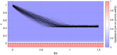
Figure 1: Safe control with an affine CBF over 200 trials. The color map shows the bounds of $P(x,150)$ for each state $x$.

5.2 Inverted Pendulum

We next consider the following case with bounded CBF, a discretized model of inverted pendulum about its upright position:

$$x_{k+1}=\begin{bmatrix}\theta_{k+1}\\ \dot{\theta}_{k+1}\end{bmatrix}=\underbrace{\begin{bmatrix}\theta_{k}+\Delta t\dot{\theta}_{k}\\ \dot{\theta}_{k}+\Delta t\sin(\theta_{k})\end{bmatrix}+\begin{bmatrix}0\\ \Delta tu_{k}\end{bmatrix}}_{F(x_{k},u_{k})}+w_{k},$$ (41)

with $\Delta t=0.01$, $\omega_{k}\sim\mathcal{N}(0,\Sigma\Delta t)$ with $\Sigma={\rm diag}\left(0.05^{2},0.25^{2}\right)$, and a quadratic CBF $h(x)=x^{\top}Ax+1$ with

$$A=-\frac{6^{2}}{\pi^{2}}\begin{bmatrix}1&3^{-\frac{1}{2}}\\ 3^{-\frac{1}{2}}&1\end{bmatrix}.$$ (42)

Here, the system dynamics and the safety set are adapted from Cosner et al. (2023).

We compare the safety bounds obtained by condition (9) in Theorem 4, condition (24) in Proposition 8, and condition (29) in Theorem 11. Condition (9) and the $K$-step exit probability (10) can then be rewritten as

$$h(F(x,u))+{\rm Tr}(A\Sigma)\geq\alpha h(x),$$ (43)

$$P(x_{0},K)\leq 1-\alpha^{K}h(x_{0}),$$ (44)

respectively, where we set $\alpha=1+{\rm Tr}(A\Sigma)$, the highest value it can take to guarantee the feasibility of (43) when $h(x)=1$.
For Proposition 8, we use $\Psi(x)=x^{2}$. Then, after performing some calculations to derive the explicit form of (24), the condition (24) and the $K$-step exit probability (26) can be rewritten as

$$(h(F)-1)^{2}+4F^{\top}A\Sigma AF+2F^{\top}AF{\rm Tr}(A\Sigma)$$

$$\hskip 10.00002pt+2{\rm Tr}((A\Sigma)^{2})+({\rm Tr}(A\Sigma))^{2}\geq(h(x)-1)^{2}+\beta$$ (45)

$$P(x_{0},K)\leq(h(x_{0})-1)^{2}+\beta K,$$ (46)

respectively, where $F=F(x,u)$. For (45), we set $\beta={\rm Tr}((A\Sigma)^{2})+({\rm Tr}(A\Sigma))^{2}$, which is the maximum value which ensures the feasibility of (45) for all $x\in\mathcal{C}$. This choice is also justified by examining the case where $x=0$ and $F(x,u)=0$. Note that (45) gives a convex constraint with respect to $u$, as also shown in Corollary 9.
For Theorem 6, similarly to Subsection 5.1, we introduce a scalar parameter $a$ to tighten the exit probability. Then, (29) and the $K$-step exit probability (33) can be rewritten as

$$ah(F)-F^{\top}aA\left(\frac{1}{2}\Sigma^{-1}+aA\right)aAF$$

$$\ \ \geq-\log(\exp(-ah(x))+\beta)-\frac{1}{2}\log\det(I+2\Sigma aA)$$ (47)

$$P(x_{0},K)\leq\exp(-ah(x_{0}))+K\beta,$$ (48)

respectively, where $F=F(x,u)$. We set $a=10$ and $\beta=10^{-5}$, values that ensure the feasibility of (47) for the case $x=0$ and $F(x,u)=0$, and consequently for all $x\in\mathcal{C}$. Note that (47) also gives a convex constraint with respect to $u$, as shown in Corollary 12.

The simulation results with $x_{0}=[0,0]^{\top}$, $u_{k}^{\rm nom}=0$ and $K=100$ for 500 trials of each method are shown in Fig. 2. Upperbounds of $P(x_{0},100)$ for Theorem 4, Proposition 8 and Theorem 11 are approximately $21.1\%$, $0.16\%$, and $0.10\%$, respectively. It can be observed that Theorem 11 yields the tightest bound, followed by Proposition 8.

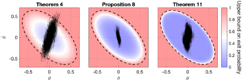
Figure 2: Safe control of an inverted pendulum using different conditions for 500 trials. The dotted lines show the boundary of the safe set $h(x)=0$, and the color map shows the bounds of $P(x,100)$ for each state $x$.

5.3 Single Integrator Obstacle Avoidance

Lastly, we consider the control of a discretized model of 2D unit-mass single-integrator dynamics, avoiding obstacles. This is a discretized model of the case considered in Singletary et al. (2021). The system dynamics is given as

$$x_{k+1}=x_{k}+u_{k}\Delta t+w_{k},$$ (49)

with $\Delta t=0.01$, $w_{k}\sim\mathcal{N}\left(0_{2},{\rm diag}\left(0.02\Delta t,0.02\Delta t\right)\right)$. We consider the case where a quadratic CBF $h(x)=x^{\top}Ax+b^{T}x+c$ yields an unbounded safe set $\mathcal{C}$. For the safe controller synthesis (23) with conditions (29) in Theorem 11, similarly to Subsections 5.1 and 5.2, we introduce a scalar parameter $a$ to tighten the exit probability.

For the nominal controller, we use a simple proportional controller with a gain of $1$ on position, defined as

$$u_{k}^{\rm nom}=-(x_{k}-x_{\rm goal}),$$ (50)

where $x_{\rm goal}\in\mathbb{R}^{2}$ represents the desired destination.

In this example, we consider safety-critical control using a single CBF as well as multiple CBFs to address complex safe sets.

5.3.1 Single CBF

We first consider the case when $h(x)=0$ is a hyperbora, defined by $A={\rm diag}\left(5,-1\right)$, $b=0_{2}$, and $c=0.3$ in the quadratic CBF $h(x)$. This case considers an unbounded safe set with unbounded barrier functions under Gaussian distributed noise, a scenario not addressed by the aforementioned existing methods. Note that the condition (29) is not convex with respect to $u$, making (23) a non-convex optimization problem. The simulation results with $x_{0}=[-2.5,1]^{\top}$, $x_{\rm goal}=[2.5,0.5]^{\top}$, $a=20$, $\beta=10^{-4}$, and $K=300$ for 200 trials are shown in Fig. 3. The upperbound for $P(x_{0},300)$ under this condition is approximately $3.00\%$. It can be observed that the system remains inside the safe region in all cases, showing the efficacy of our proposed method.

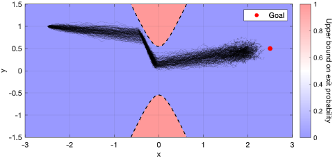
Figure 3: Safe control of a single integrator model using Theorem 6 for 200 trials. The dotted line shows the boundary of the safe set $h(x)=0$, and the color map shows the bounds of $P(x,300)$ for each state $x$.

5.3.2 Multiple CBFs

Next, we consider a scenario in which the system must avoid $l$ obstacles, each represented by a distinct CBF, $h_{i}(x)$, $i=1,\dots l$. Then, the safe set $\mathcal{C}$ can be defined as

$$\mathcal{C}=\{x\in\mathbb{R}^{n}\mid\ \forall i=1,\dots,l,\ h_{i}(x)\geq 0\}.$$ (51)

In this case, we can evaluate the $K$-step exit probability bound for $\mathcal{C}$ by evaluating $K$-step exit probability bound for each subset of the safe set given by

$$\mathcal{C}_{i}=\{x\in\mathbb{R}^{n}\mid\ h_{i}(x)\geq 0\}.$$ (52)

Theorem 6 yields $K$-step exit probability bound for each $\mathcal{C}_{i}$ by designing a function $\Phi_{i}$ as the auxiliary function of $h_{i}$, as

$$P_{\mathcal{C}_{i}}\left(x_{0},K\right) :=\mathbb{P}\left(\min_{0\leq k\leq K}h_{i}(x_{k})<0\right)$$ (53)

$$\leq\frac{\Phi_{i}(h_{i}(x_{0}),0)}{\min_{0\leq k\leq K}\Phi_{i}(0,k)}.$$

Then, by applying Boole’s inequality, we obtain a bound of the $K$-step exit probability for the safe set $\mathcal{C}$ from the bounds of probabilities for $\mathcal{C}_{i}$, as

$$\mathbb{P}\left(\min_{0\leq k\leq K,i=1,\dots l}h_{i}(x_{k})<0\right)=\mathbb{P}\left(\bigcup_{i=1}^{l}\min_{0\leq k\leq K}h_{i}(x_{k})<0\right)$$

$$\leq\sum_{i=1}^{l}P_{\mathcal{C}_{i}}(x_{0},K)\leq\sum_{i=1}^{l}\frac{\Phi_{i}(h_{i}(x_{0}),0)}{\min_{0\leq k\leq K}\Phi_{i}(0,k)}.$$ (54)

We consider avoiding four circular obstacles, each with a radius of $0.4$, centered at $[-1.5,0.7]^{\top}$, $[0.5,0.7]^{\top}$, $[-0.5,-0.7]^{\top}$, and $[1.5,-0.7]^{\top}$, respectively. For the corresponding CBFs, we set $A_{i}=I_{2}$ and define $b_{i},c_{i}$ for $i=1,\dots,4$, accordingly. Here, similary to the single CBF cases, it can be seen that the bound on the $K$-step exit probability can be tightened by introducing scalar parameters $a_{i}$ and consider $a_{i}h_{i}(x)$ in (54). We set $a_{i}=20$ and $\beta_{i}=10^{-5}$ for all $i=1,\dots 4$.

The simulation results with $x_{0}=[-2.5,0.5]^{\top}$, $x_{\rm goal}=[2.5,-0.5]^{\top}$, and $K=300$ for 200 trials are shown in Fig. 4. The upperbound for $P(x_{0},300)$ under this condition is approximately $0.30\%$. It can be observed that the system remains inside the safe region for all trials, showing the efficacy of our proposed method.

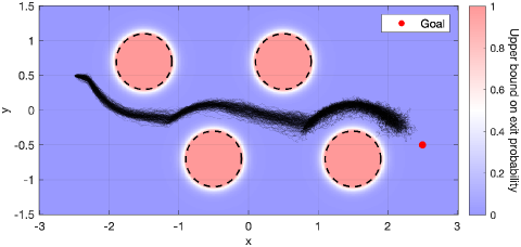
Figure 4: Safe control of a single integrator model using Theorem 6 for 200 trials. The dotted line shows the boundary of the safe set $h(x)=0$, and the color map shows the bounds of $P(x,300)$ for each state $x$.

6 CONCLUSION

In this work, we presented conditions for probabilistically safe controller synthesis in stochastic systems to provide flexible bounds of the safe probability. Future directions include exploring more constructive methods for determining parameters in the design of controllers, and extending this approach to more complex scenarios such as continuous-time stochastic systems as in Hoshino et al. (2023); Nishimura and Hoshino (2024), and comparing with non-martingale-based finite-time safety guarantee method such as Black et al. (2023) and Liu et al. (2024).

References

- Agrawal and Sreenath (2017) Agrawal, A. and Sreenath, K. (2017). Discrete control barrier functions for safety-critical control of discrete systems with application to bipedal robot navigation. In Robotics: Science and Systems, volume 13, 1–10. Cambridge, MA, USA.
- Ames et al. (2019) Ames, A.D., Coogan, S., Egerstedt, M., Notomista, G., Sreenath, K., and Tabuada, P. (2019). Control barrier functions: Theory and applications. In 2019 18th European control conference (ECC), 3420–3431. IEEE.
- Black et al. (2023) Black, M., Fainekos, G., Hoxha, B., Prokhorov, D., and Panagou, D. (2023). Safety under uncertainty: Tight bounds with risk-aware control barrier functions. In 2023 IEEE International Conference on Robotics and Automation (ICRA), 12686–12692. IEEE.
- Cosner et al. (2024) Cosner, R.K., Culbertson, P., and Ames, A.D. (2024). Bounding stochastic safety: Leveraging freedman’s inequality with discrete-time control barrier functions. IEEE Control Systems Letters.
- Cosner et al. (2023) Cosner, R.K., Culbertson, P., Taylor, A.J., and Ames, A.D. (2023). Robust safety under stochastic uncertainty with discrete-time control barrier functions. arXiv preprint arXiv:2302.07469.
- Hoshino et al. (2023) Hoshino, K., Wang, Z., and Nakahira, Y. (2023). Scalable long-term safety certificate for large-scale systems. IEEE Control Systems Letters, 7, 1285–1290.
- Kushner (1966) Kushner, H. (1966). Finite time stochastic stability and the analysis of tracking systems. IEEE Transactions on Automatic Control, 11(2), 219–227.
- Kushner (1967) Kushner, H.J. (1967). Stochastic stability and control.
- Liu et al. (2024) Liu, Z., Jafarpour, S., and Chen, Y. (2024). Safety verification of stochastic systems: A set-erosion approach. IEEE Control Systems Letters.
- Nishimura and Hoshino (2024) Nishimura, Y. and Hoshino, K. (2024). Control barrier functions for stochastic systems and safety-critical control designs. IEEE Transactions on Automatic Control.
- Prajna et al. (2007) Prajna, S., Jadbabaie, A., and Pappas, G.J. (2007). A framework for worst-case and stochastic safety verification using barrier certificates. IEEE Transactions on Automatic Control, 52(8), 1415–1428.
- Santoyo et al. (2021) Santoyo, C., Dutreix, M., and Coogan, S. (2021). A barrier function approach to finite-time stochastic system verification and control. Automatica, 125, 109439.
- Singletary et al. (2021) Singletary, A., Klingebiel, K., Bourne, J., Browning, A., Tokumaru, P., and Ames, A. (2021). Comparative analysis of control barrier functions and artificial potential fields for obstacle avoidance. In 2021 IEEE/RSJ International Conference on Intelligent Robots and Systems (IROS), 8129–8136. IEEE.
- So et al. (2023) So, O., Clark, A., and Fan, C. (2023). Almost-sure safety guarantees of stochastic zero-control barrier functions do not hold. arXiv preprint arXiv:2312.02430.
- Steinhardt and Tedrake (2012) Steinhardt, J. and Tedrake, R. (2012). Finite-time regional verification of stochastic non-linear systems. The International Journal of Robotics Research, 31(7), 901–923.
- Ville (1939) Ville, J. (1939). Etude critique de la notion de collectif.
- Zikelic et al. (2023) Zikelic, D., Lechner, M., Henzinger, T.A., and Chatterjee, K. (2023). Learning control policies for stochastic systems with reach-avoid guarantees. In Proceedings of the AAAI Conference on Artificial Intelligence, volume 37, 11926–11935.