General detectability measure

Abstract

Distinguishing resource states from resource-free states is a fundamental task in quantum information. We have approached the state detection problem through a hypothesis testing framework, with the alternative hypothesis set comprising resource-free states in a general context. Consequently, we derived the optimal exponential decay rate of the failure probability for detecting a given $n$-tensor product state when the resource-free states are separable states, positive partial transpose (PPT) states, or the convex hull of the set of stabilizer states. This optimal exponential decay rate is determined by the minimum of the reverse relative entropy, indicating that this minimum value serves as the general detectability measure. The key technique of this paper is a quantum version of empirical distribution.

I Introduction

In quantum information theory, various resources play crucial roles, such as entangled states (non-separable states), non-positive partial transpose (non-PPT) states, and magic states (non-stabilizer states) [1, 2, 3]. These resource states are characterized by their exclusion from specific convex cones, for example, the cone of separable states, the cone of PPT states, and the cone of stabilizer states. Consequently, verifying whether a given state lies outside a particular convex cone is of fundamental importance. Recently, the paper [4] proposed that such a detection problem can be framed as a hypothesis testing problem where the alternative hypothesis $H_{1}$ is composite, consisting of states in a given convex cone, and the null hypothesis $H_{0}$ corresponds to the specific state under detection. When $H_{1}$ is defined as the set of $n$-tensor product states, this hypothesis testing problem has been studied under the framework of the quantum Sanov theorem [5, 6] although the paper [7] showed that the asymptotically optimal measurement can be chosen depending only on the null hypothesis $H_{0}$. The paper [4] explored the relationship between the reverse relative entropy of entanglement and the exponential rate of decrease in the non-detection probability, proving the equality for maximally correlated states. Subsequently, the works [8, 9] extended this equality to general entangled states, addressing the hypothesis testing problem within general frameworks. The paper [8] covers the case of separable states. However, these papers did not investigate non-PPT states or magic (non-stabilizer) states. In particular, although [9] developed a general theory for this hypothesis testing problem, it demonstrated that PPT states do not satisfy their general condition [9, Discussion after Eq. (334)]. In addition, hypothesis testing has a close relation with various problems in quantum information, e.g., classical-quantum channel coding [10, 11], entanglement distillation [12, 13], [14, Theorem 8.7], quantum data compression [15],[14, Lemma 10.3],[16, Remark 16], quantum resource theory [17, 18], and classical-quantum arbitrarily varying channel [19, 20], etc. In particular, the references [10, 13, 14, 15, 16] linked the respective topics to quantum hypothesis testing via the method of quantum information spectrum.

In this paper, we introduce a comprehensive method to handle this hypothesis testing problem within a general framework. Assuming broad conditions, we derive the exponential decay rate of the non-detection probability, which equals the minimum of the reverse relative entropy over various non-resource states. This minimum value serves as a general detectability measure. Our conditions involve the existence of a compatible measurement, as defined in [21], alongside partial conditions from [22]. The compatible measurement must also be tomography-complete [23]. While the paper [8] imposes a condition related to compatible measurements, our condition is considerably simpler and easier to verify. Specifically, the sets of separable states, PPT states, and the convex hull of stabilizer states satisfy our conditions.

A pivotal component of our method is the quantum version of empirical distribution, introduced in [4] to formulate an alternative quantum Sanov theorem. Hence, we begin by distinguishing between the two types of quantum Sanov theorems from [5, 6] and [4]. Empirical distribution plays a central role in information theory and statistics. The original classical Sanov theorem [24, 25] characterizes its asymptotic behavior under the i.i.d. condition, providing the exponential decay rate for events where the empirical distribution belongs to a subset excluding the true distribution.

In the quantum context, analogous i.i.d. conditions are considered through $n$-fold tensor products. However, defining a quantum analog of empirical distribution is nontrivial. The papers [5, 6] introduced a version of the quantum Sanov theorem without quantum empirical distributions. They framed a hypothesis testing problem where one hypothesis is a composite set of i.i.d. states, and the other is a single i.i.d. state because the performance of this hypothesis testing can be easily derived from the original Sanov theorem under the classical setting. The exponential decay rate for error probability was derived under a constant constraint on the composite hypothesis error probability. This result was termed the quantum Sanov theorem. The paper [4] refined this analysis by applying an exponential constraint instead.

The quantum Sanov theorem by [5, 6] has the following problem. When we extend a proof-technique-based on empirical distributions to a quantum setting, this version of quantum Sanov theorem does not work well. That is, to extend such a proof-technique to a quantum case, we need to establish a quantum version of empirical distributions, and their asymptotic behavior. For instance, [26] used empirical distributions to analyze channel resolvability’s second-order asymptotics. Extending such results requires a quantum empirical distribution framework. The paper [27] provided an alternative quantum Sanov theorem, establishing quantum empirical distributions’ asymptotic behavior. Using this result, the paper [28] proved strong converse results for classical-quantum channel resolvability. Therefore, we refer to the papers [5, 6]’s result as the quantum Sanov theorem for hypothesis testing and the paper [27]’s as the quantum Sanov theorem for quantum empirical distributions.

In this paper, we leverage the latter for general hypothesis testing with composite hypotheses. First, we address classical composite hypotheses under permutation symmetry using empirical distributions. This approach directly applies the classical Sanov theorem, where permutation symmetry reduces sufficient statistics to empirical distributions. Although our conditions initially involve empirical distribution properties, we simplify them by using compatibility conditions from [21], making verification straightforward. Next, we extend this framework to quantum hypothesis testing by using quantum empirical distributions. Our method reproduces the same exponential decay rate as that by [8, 9], i.e., the general detectability measure, while requiring simpler conditions. Although verifying the separable state condition is nontrivial in the paper [8], our condition is immediately satisfied. This demonstrates the practicality of our approach and the relevance of quantum empirical distributions in hypothesis testing.

The structure of this paper is as follows. Section II introduces the formulation and key notations. Section III outlines existing results and our main findings, showing that separable states, PPT states, and stabilizer state convex hulls meet our assumptions. Sections IV and V detail classical generalizations by using two methods, both serving as precursors to our final results. Section VI reviews the quantum Sanov theorem for quantum empirical distributions and presents newly obtained and related formulas. Finally, Section VII presents our main quantum generalization of the quantum Sanov theorem for hypothesis testing.

II Preparation

II.1 Formulation

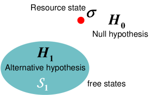
Figure 1: Our testing problem

In this paper, we study the problem of quantum hypothesis testing to distinguish a given state $\sigma$ from a set ${\cal S}_{1}$ of resource-free states. In the standard framework of quantum hypothesis testing, two quantum states, $\rho$ and $\sigma$, on a given Hilbert space ${\cal H}$ represent the two simple hypotheses. As illustrated in Fig. 1, one is the alternative hypothesis $H_{1}$, which is composed of a state $\rho$, the is the null hypothesis $H_{0}$, which is composed of a state $\sigma$. The aim of the hypothesis testing is to accept the null hypothesis $H_{0}$ by rejecting $H_{1}$ with a fixed precision level. To keep this fixed precision level for the rejection of $H_{1}$, we impose the probability for incorrectly rejecting $H_{1}$ to be upper bounded by a threshold $\epsilon>0$. That is, we impose the following condition for our test operator $T$ as

$${\cal D}_{\epsilon,\rho}\coloneqq\Big{\{}T\Big{|}0\leq T\leq I,\Tr[(I-T)\rho]\leq\epsilon\Big{\}},$$ (1)

where $I$ denotes the identity operator. Then, we optimize our test under this condition as follows.

$$\beta_{\epsilon}(\rho\|\sigma)\coloneqq\min_{T\in{\cal D}_{\epsilon,\rho}}\Tr[T\sigma].$$ (2)

Since our aim is to distinguish a given state $\sigma$ from a compact set ${\cal S}_{1}$ of resource-free states, we impose the following condition instead of (1).

$${\cal D}_{\epsilon,\mathcal{S}_{1}}\coloneqq\Big{\{}T\Big{|}0\leq T\leq I,\max_{\rho\in\mathcal{S}_{1}}\Tr[(I-T)\rho]\leq\epsilon\Big{\}}.$$ (3)

A hypothesis characterized by a set of states is known as a “composite hypothesis”. Our optimization problem is formulated as

$$\beta_{\epsilon}\left(\mathcal{S}_{1}\middle\|\sigma\right)\coloneqq\min_{T\in{\cal D}_{\epsilon,\mathcal{S}_{1}}}\Tr[T\sigma].$$ (4)

This quantity can be generalized by using another compact set of states $\mathcal{S}_{2}$ as

$$\beta_{\epsilon}\left(\mathcal{S}_{1}\middle\|\mathcal{S}_{2}\right)\coloneqq\min_{T\in{\cal D}_{\epsilon,\mathcal{S}_{1}}}\max_{\sigma\in\mathcal{S}_{2}}\Tr[T\sigma].$$ (5)

For convenience, we introduce the following auxiliary quantities:

$$\beta_{\epsilon}(\rho\|{\cal S}_{2})\coloneqq\max_{0\leq T\leq I}\Big{\{}\max_{\sigma\in{\cal S}_{2}}\Tr[\sigma T]\Big{|}\Tr[(I-T)\rho]\leq\epsilon\Big{\}}.$$ (6)

We also employ the relative entropy and the sandwiched Rényi relative entropy [29, 30], defined as

$$D(\rho\|\sigma) \coloneqq\Tr\rho(\log\rho-\log\sigma),$$ (7)

$$D_{\alpha}(\rho\|\sigma) \coloneqq\frac{1}{\alpha-1}\log\Tr\left(\sigma^{\frac{1-\alpha}{2\alpha}}\rho\sigma^{\frac{1-\alpha}{2\alpha}}\right)^{\alpha}.$$ (8)

Specifically, $D_{1}(\rho\|\sigma)$ is equivalent to the relative entropy $D(\rho\|\sigma)$.

In preparation for the following discussion, we define the notations:

$$D_{\alpha}(\mathcal{S}_{1}\|\sigma) \coloneqq\min_{\rho\in\mathcal{S}_{1}}D_{\alpha}(\rho\|\sigma),$$ (9)

$$D_{\alpha}(\rho\|\mathcal{S}_{2}) \coloneqq\min_{\sigma\in\mathcal{S}_{2}}D_{\alpha}(\rho\|\sigma),$$ (10)

$$D_{\alpha}(\mathcal{S}_{1}\|\mathcal{S}_{2}) \coloneqq\min_{\rho\in\mathcal{S}_{1},\sigma\in\mathcal{S}_{2}}D_{\alpha}(\rho\|\sigma).$$ (11)

In addition, in this paper, $\{X\geq Y\}$ expresses the projection $\sum_{j\mathrel{\mathop{\ordinarycolon}}z_{j}\geq 0}E_{j}$, where $X-Y=\sum_{j}z_{j}E_{j}$.

II.2 Basic Lemmas

Before proceeding with detailed analysis, we present basic lemmas. Using the max-min inequality [31, Section 5.4.1], we obtain

$$\max_{\sigma\in\mathcal{S}_{2}}\beta_{\epsilon}\left(\mathcal{S}_{1}\middle\|\sigma\right)\leq\beta_{\epsilon}\left(\mathcal{S}_{1}\middle\|\mathcal{S}_{2}\right).$$ (12)

When $\mathcal{S}_{2}$ is convex, the minimax theorem [32, 33, 34] yields the following results:

Lemma 1.

For any $\epsilon\geq 0$, any compact set $\mathcal{S}_{1}$, any convex compact set $\mathcal{S}_{2}$, and any state $\rho$, the following hold:

$$\max_{\sigma\in\mathcal{S}_{2}}\beta_{\epsilon}\left(\rho\middle\|\sigma\right) =\beta_{\epsilon}\left(\rho\middle\|\mathcal{S}_{2}\right),$$ (13)

$$\max_{\sigma\in\mathcal{S}_{2}}\beta_{\epsilon}\left(\mathcal{S}_{1}\middle\|\sigma\right) =\beta_{\epsilon}\left(\mathcal{S}_{1}\middle\|\mathcal{S}_{2}\right).$$ (14)

Additionally, for any $\epsilon\geq 0$, any convex compact sets $\mathcal{S}_{1}$ and $\mathcal{S}_{2}$, and any state $\sigma$, the following hold:

$$\max_{\rho\in\mathcal{S}_{1}}\beta_{\epsilon}\left(\rho\middle\|\sigma\right) =\beta_{\epsilon}\left(\mathcal{S}_{1}\middle\|\sigma\right),$$ (15)

$$\max_{\rho\in\mathcal{S}_{1}}\beta_{\epsilon}\left(\rho\middle\|\mathcal{S}_{2}\right) =\beta_{\epsilon}\left(\mathcal{S}_{1}\middle\|\mathcal{S}_{2}\right).$$ (16)

Proof.

The convexity and compactness of ${\cal D}_{\epsilon,\rho}$ allow us to derive (13) from the minimax theorem [32, 33, 34], as shown in Lemma 3 of Ref. [18]. Similarly, (14) follows from the convexity and compactness of ${\cal D}_{\epsilon,\mathcal{S}_{1}}$, as demonstrated in Ref. [18].

We now establish (15). Let

$$\alpha\coloneqq\max_{\rho\in\mathcal{S}_{1}}\beta_{\epsilon}\left(\rho\middle\|\sigma\right).$$ (17)

Since ${\cal D}_{\epsilon,\mathcal{S}_{1}}\subseteq{\cal D}_{\epsilon,\rho}$ for all $\rho\in\mathcal{S}_{1}$, we have

$$\beta_{\epsilon}\left(\rho\middle\|\sigma\right)\leq\beta_{\epsilon}\left(\mathcal{S}_{1}\middle\|\sigma\right),$$ (18)

implying

$$\alpha\leq\beta_{\epsilon}\left(\mathcal{S}_{1}\middle\|\sigma\right).$$ (19)

For any $\rho\in\mathcal{S}_{1}$, the inequality $\beta_{\epsilon}\left(\rho\middle\|\sigma\right)\leq\alpha$ leads to

$$\beta_{\alpha}\left(\sigma\middle\|\rho\right)\leq\epsilon.$$ (20)

Since $\mathcal{S}_{1}$ is convex, (14) implies

$$\beta_{\alpha}\left(\sigma\middle\|\mathcal{S}_{1}\right)=\max_{\rho\in\mathcal{S}_{1}}\beta_{\alpha}\left(\sigma\middle\|\rho\right)\leq\epsilon.$$ (21)

Thus, there exists a POVM $\{T^{\ast},I-T^{\ast}\}$ such that

$$\max_{\rho\in\mathcal{S}_{1}}\Tr[T^{\ast}\rho]\leq\epsilon,\quad\Tr[(I-T^{\ast})\sigma]\leq\alpha.$$ (22)

This implies

$$\beta_{\epsilon}\left(\mathcal{S}_{1}\middle\|\sigma\right)\leq\Tr[(I-T^{\ast})\sigma]\leq\alpha.$$ (23)

Combining (19) and (23), we obtain (15).

Finally, (16) follows from (13), (14), and (15), since

$$\max_{\rho\in\mathcal{S}_{1}}\beta_{\epsilon}\left(\rho\middle\|\mathcal{S}_{2}\right)=\max_{\rho\in\mathcal{S}_{1}}\max_{\sigma\in\mathcal{S}_{2}}\beta_{\epsilon}\left(\rho\middle\|\sigma\right)$$

$$= \max_{\sigma\in\mathcal{S}_{2}}\max_{\rho\in\mathcal{S}_{1}}\beta_{\epsilon}\left(\rho\middle\|\sigma\right)=\max_{\sigma\in\mathcal{S}_{2}}\beta_{\epsilon}\left(\mathcal{S}_{1}\middle\|\sigma\right)=\beta_{\epsilon}\left(\mathcal{S}_{1}\middle\|\mathcal{S}_{2}\right).$$ (24)

∎

When sets $\mathcal{S}_{1}$ and $\mathcal{S}_{2}$ are convex and closed for a unitary representation $U$ of a group, the joint convexity of relative entropy guarantees

$$D\left(\mathcal{S}_{1}\middle\|\mathcal{S}_{2}\right)=D\left(\mathcal{S}_{1,inv}\middle\|\mathcal{S}_{2,inv}\right),$$ (25)

where we denote the set of invariant elements for $U$ in ${\cal S}_{j}$ by ${\cal S}_{j,inv}$ for $j=1,2$. The minimum error probability also satisfies the same property as follows.

Lemma 2.

Given a unitary representation $U$ of a group $G$ on ${\cal H}$, we assume that the sets $\mathcal{S}_{1}$ and $\mathcal{S}_{2}$ are convex and closed for $U$. Then, we have

$$\beta_{\epsilon}\left(\mathcal{S}_{1}\middle\|\mathcal{S}_{2}\right)=\beta_{\epsilon}\left(\mathcal{S}_{1,inv}\middle\|\mathcal{S}_{2,inv}\right).$$ (26)

Further, since any elements in $\mathcal{S}_{1,inv}$ and $\mathcal{S}_{2,inv}$ are invariant for $U$, our test can be limited to invariant tests.

Proof.

Since ${\cal S}_{1}$ is a closed set for $U$, the set ${\cal D}_{\epsilon,\mathcal{S}_{1}}$ is also closed for $U$. Hence, we have

$$\beta_{\epsilon}\left(\mathcal{S}_{1}\middle\|\sigma\right)=\beta_{\epsilon}\left(\mathcal{S}_{1}\middle\|U(g)\sigma U(g)^{\dagger}\right)$$ (27)

for $g\in G$. Thus, we have

$$\beta_{\epsilon}\left(\mathcal{S}_{1}\middle\|\sum_{g\in G}\frac{1}{|G|}U(g)\sigma U(g)^{\dagger}\right)$$

$$\geq \sum_{g\in G}\frac{1}{|G|}\beta_{\epsilon}\left(\mathcal{S}_{1}\middle\|U(g)\sigma U(g)^{\dagger}\right)=\beta_{\epsilon}\left(\mathcal{S}_{1}\middle\|\sigma\right).$$ (28)

Since $\sum_{g\in G}\frac{1}{|G|}U(g)\sigma U(g)^{\dagger}$ is an invariant element in $\mathcal{S}_{2}$, we have

$$\beta_{\epsilon}\left(\mathcal{S}_{1}\middle\|\mathcal{S}_{2}\right)=\max_{\sigma\in\mathcal{S}_{2}}\beta_{\epsilon}\left(\mathcal{S}_{1}\middle\|\sigma\right)=\max_{\sigma\in\mathcal{S}_{2,inv}}\beta_{\epsilon}\left(\mathcal{S}_{1}\middle\|\sigma\right).$$ (29)

When $\sigma$ is an invariant state for $U$, we have

$$\beta_{\epsilon}\left(U(g)\rho U(g)^{\dagger}\middle\|\sigma\right)=\beta_{\epsilon}\left(\rho\middle\|\sigma\right).$$ (30)

Hence,

$$\beta_{\epsilon}\left(\sum_{g\in G}\frac{1}{|G|}U(g)\rho U(g)^{\dagger}\middle\|\sigma\right)$$

$$\geq \sum_{g\in G}\frac{1}{|G|}\beta_{\epsilon}\left(U(g)\rho U(g)^{\dagger}\middle\|\sigma\right)=\beta_{\epsilon}\left(\rho\middle\|\sigma\right).$$ (31)

Since $\sum_{g\in G}\frac{1}{|G|}U(g)\rho U(g)^{\dagger}$ is an invariant element in $\mathcal{S}_{1}$, we have

$$\beta_{\epsilon}\left(\mathcal{S}_{1}\middle\|\sigma\right)=\max_{\rho\in\mathcal{S}_{1}}\beta_{\epsilon}\left(\rho\middle\|\sigma\right)$$

$$= \max_{\rho\in\mathcal{S}_{1,inv}}\beta_{\epsilon}\left(\rho\middle\|\sigma\right)=\beta_{\epsilon}\left(\mathcal{S}_{1,inv}\middle\|\rho\right).$$ (32)

The combination of (109) and (32) yields

$$\beta_{\epsilon}\left(\mathcal{S}_{1}\middle\|\mathcal{S}_{2}\right)=\max_{\sigma\in\mathcal{S}_{2,inv}}\beta_{\epsilon}\left(\mathcal{S}_{1}\middle\|\sigma\right)$$

$$= \max_{\sigma\in\mathcal{S}_{2,inv}}\beta_{\epsilon}\left(\mathcal{S}_{1,inv}\middle\|\sigma\right)=\beta_{\epsilon}\left(\mathcal{S}_{1,inv}\middle\|\mathcal{S}_{2,inv}\right).$$ (33)

∎

III Our results and existing results

III.1 Existing results

Before presenting our results, we review existing results. We consider a $d$-dimensional system ${\cal H}$ spanned by the computational basis $\{|j\rangle\}_{j=1}^{d}$. and the set of density matrices on ${\cal H}$, which is denoted by ${\cal S}({\cal H})$. We denote the set of diagonal states with respect to the computation basis by ${\cal S}_{c}({\cal H})$. We focus on a sequence of subsets ${\cal F}_{n}\subset{\cal S}({\cal H}^{\otimes n})$. According to the paper [22], the paper [8] considers the following conditions

(A1)

Each ${\cal F}_{n}$ is a convex and closed subset of ${\cal S}({\cal H}^{\otimes n})$, and hence also compact.

(A2)

${\cal F}_{1}$ contains some full-rank state $\sigma_{0}(\geq e^{-r_{0}}>0)\in{\cal F}_{1}$.

(A3)

The family ${\cal F}_{n}$ is closed under partial traces, i.e. if $\sigma\in{\cal F}_{n}$ then $\Tr_{n}\sigma\in{\cal F}_{n-1}$ and $\Tr_{1,\ldots,n-1}\sigma\in{\cal F}_{1}$, where $\Tr_{n}$ denotes the partial trace over the $n$-th subsystem and $\Tr_{1,\ldots,n-1}$ denotes the partial trace over the $1$st, $2$nd,$\ldots$, $n-1$-th subsystems.

(A4)

The family ${\cal F}_{n}$ is closed under tensor products, i.e. if $\sigma\in{\cal F}_{n}$ and $\sigma^{\prime}\in{\cal F}_{m}$ then $\sigma\otimes\sigma^{\prime}\in{\cal F}_{n+m}$.

(A5)

Each ${\cal F}_{n}$ is closed under permutations, i.e. if $\sigma\in{\cal F}_{n}$ and $\pi\in{\cal S}_{n}$ denotes an arbitrary permutation of a set of $n$ elements, then also $U_{\pi}\sigma U_{\pi}^{\dagger}\in{\cal F}_{n}$, where $U_{\pi}$ is the unitary implementing $\pi$ over ${\cal H}^{\otimes n}$. Under this condition, we denote the set of permutation-invariant states in ${\cal F}_{n}$ by ${\cal F}_{n,inv}$.

Recently, the paper [8] introduced the following condition.

(A6)

The regularised relative entropy of resource is faithful, i.e. For any element $\rho\notin{\cal F}_{1}$, we have

$$D^{\infty}(\rho\|{\cal F})\mathrel{\mathop{\ordinarycolon}}=\lim_{n\to\infty}\frac{1}{n}D(\rho^{\otimes n}\|{\cal F}_{n})>0.$$ (34)

The paper [8] showed the following statement as a classical extension of quantum Sanov theorem for hypothesis testing.

Proposition 3.

[8, Theorem 8] When a sequence of subsets ${\cal F}_{n}\subset{\cal S}_{c}({\cal H}^{\otimes n})$ satisfies the conditions (A1)–(A6), any state $\sigma\in{\cal S}_{c}({\cal H})$ satisfies

$$\lim_{n\to\infty}-\frac{1}{n}\log\beta_{\epsilon}({\cal F}_{n}\|\sigma^{\otimes n})=D({\cal F}_{1}\|\sigma)=\lim_{n\to\infty}\frac{1}{n}D({\cal F}_{n}\|\sigma^{\otimes n}).$$ (35)

Definition 1.

[21, Definition 4] A POVM $M=\{M_{j}\}_{j}$ on ${\cal H}$ is called compatible with $({\cal F}_{n})_{n}$ when $\Tr_{n}(I^{\otimes n-1}\otimes M_{j})\rho_{n}/\Tr(I^{\otimes n-1}\otimes M_{j})\rho_{n}$ belongs to ${\cal F}_{n-1}$ for $\rho_{n}\in{\cal F}_{n}$.

Also, the paper [8] introduced the following condition.

(A7)

There exists a sequence $r_{n}\in(0,1]$ to satisfy the following condition. We define the set ${\cal M}_{n}$ of POVMs as

$${\cal M}_{n}\mathrel{\mathop{\ordinarycolon}}=\Big{\{}\Big{\{}\frac{1}{2}(I^{\otimes n}+X_{n}),\frac{1}{2}(I^{\otimes n}-X_{n})\Big{\}}\Big{|}\|X_{n}\|\leq r_{n}\Big{\}}.$$ (36)

Any POVM in ${\cal M}_{n}$ is compatible with $({\cal F}_{n})_{n}$.

The paper [8] showed the following statement as a quantum extension of quantum Sanov theorem for hypothesis testing.

Proposition 4.

[8, Theorem 14] When a sequence of subsets ${\cal F}_{n}\subset{\cal S}({\cal H}^{\otimes n})$ satisfies the conditions (A1)-(A5) and (A7), any state $\sigma$ satisfies (35).

Later, the paper [9] considered another condition. For a set ${\cal F}$, they define the subset

$$({\cal F})_{+}^{\circ}\mathrel{\mathop{\ordinarycolon}}=\{X\geq 0|\Tr XY\leq 1,\forall\in{\cal F}\}.$$ (37)

Then, the paper [9] introduced the condition;

(A8)

The relation

$$({\cal F}_{n})_{+}^{\circ}\otimes({\cal F}_{m})_{+}^{\circ}\subset({\cal F}_{n+m})_{+}^{\circ}$$ (38)

holds for any two positive integers $n,m$.

The paper [9] showed the following statement as another quantum extension of quantum Sanov theorem for hypothesis testing.

Proposition 5.

[9, Theorem 26] When a sequence of subsets ${\cal F}_{n}\subset{\cal S}({\cal H}^{\otimes n})$ satisfies the conditions (A1), (A4), (A5), and (A8), any state $\sigma$ satisfies (35).

Proposition 6.

[18, Theorem 1] Assume that a sequence of subsets ${\cal F}_{n}\subset{\cal S}({\cal H}^{\otimes n})$ satisfies the conditions (A1), (A2), and (A4). For any state $\sigma$, the limits $\lim_{n\to\infty}-\frac{1}{n}\log\beta_{\epsilon}(\sigma^{\otimes n}\|{\cal F}_{n})$ and $\lim_{n\to\infty}\frac{1}{n}D(\sigma^{\otimes n}\|{\cal F}_{n})$ exist, and the relation

$$\lim_{n\to\infty}-\frac{1}{n}\log\beta_{\epsilon}(\sigma^{\otimes n}\|{\cal F}_{n})=\lim_{n\to\infty}\frac{1}{n}D(\sigma^{\otimes n}\|{\cal F}_{n})$$ (39)

holds.

III.2 Our results

To state our obtained result for the classical setting, we introduce the following condition for a sequence of subsets ${\cal F}_{n}\subset{\cal S}_{c}({\cal H}^{\otimes n})$ by strengthening the condition (A3).

(B1)

The measurement based on the computation basis is compatible with the sequence of subsets ${\cal F}_{n}\subset{\cal S}_{c}({\cal H}^{\otimes n})$. That is, all elements of ${\cal F}_{n}$ are diagonal states. For any element $\rho_{n}\in{\cal F}_{n}$, $\Tr_{1,\ldots,n-1}\rho_{n}\in{\cal F}_{1}$ and the state $\Tr_{n}\rho_{n}(I^{\otimes n-1}\otimes|j\rangle\langle j|)/\Tr\rho_{n}(I^{\otimes n-1}\otimes|j\rangle\langle j|)$ belongs to ${\cal F}_{n-1}$. That is, any conditional distribution of $\rho_{n}$ with condition on the $n$-th system belongs to ${\cal F}_{n-1}$.

Theorem 7.

When a sequence of subsets ${\cal F}_{n}\subset{\cal S}_{c}({\cal H}^{\otimes n})$ satisfies the conditions (A1), (A4), (A5), and (B1), any state $\sigma$ satisfies satisfies (35).

To state our obtained result for the quantum setting, we introduce the following definition.

Definition 2.

A POVM $M=\{M_{j}\}_{j}$ on ${\cal H}$ is called tomography-complete when the set $\{M_{j}\}$ forms a basis on the set of Hermitian matrices on ${\cal H}$ [23]. Given a state $\rho$ on ${\cal H}$, the classical state $\sum_{j}(\Tr M_{j}\rho)|j\rangle\langle j|$ by $M(\rho)$.

Then, we introduce the following condition for a sequence of subsets ${\cal F}_{n}\subset{\cal S}({\cal H}^{\otimes n})$.

(B2)

There exists a tomography-complete POVM $M=\{M_{j}\}_{j}$ on ${\cal H}$ with finite measurement outcomes such that $(M^{\otimes n}({\cal F}_{n}))_{n}$ satisfies the condition (B1).

The following condition implies the condition (B2) when the condition (A5) holds.

(B3)

There exists a tomography-complete POVM $M=\{M_{j}\}_{j}$ on ${\cal H}$ that is compatible with $({\cal F}_{n})_{n}$.

Although (B3) is a stronger condition than (B2), (B3) can be more easily checked than (B2). Hence, we often check (B3) instead of (B2). Our main result is given as follows.

Theorem 8.

When a sequence of subsets ${\cal F}_{n}\subset{\cal S}({\cal H}^{\otimes n})$ satisfies the conditions (A1), (A4), (A5), and (B2), any state $\sigma$ satisfies (35).

Further, we can show that the condition (A7) implies (B3) as follows. There exists a finite set of Hermitian matrices ${\cal W}_{n}$ such that the set ${\cal W}_{n}$ linearly spans the set of Hermitian matrices on ${\cal H}^{\otimes n}$ and any element $X_{n}\in{\cal W}_{n}$ satisfies $\|X_{n}\|\leq r_{n}$. The condition (A7) guarantees that the POVM $\Big{\{}\frac{1}{2}(I^{\otimes n}+X_{n}),\frac{1}{2}(I^{\otimes n}-X_{n})\Big{\}}$ is compatible with $({\cal F}_{n})_{n}$ for $X_{n}\in{\cal W}_{n}$. Then, the POVM $\Big{\{}\frac{1}{2l}(I^{\otimes n}+X_{n}),\frac{1}{2}(I^{\otimes n}-X_{n})\Big{\}}_{X_{n}\in{\cal W}_{n}}$ with $l=|{\cal W}_{n}|$ is compatible with $({\cal F}_{n})_{n}$ and tomography-complete, which implies the condition (B3). Therefore, the condition of Theorem 8 is a weaker condition than Proposition 3.

Theorem 8 states the equality between $D({\cal F}_{1}\|\sigma)$ and $\lim_{n\to\infty}\frac{1}{n}D({\cal F}_{n}\|\sigma^{\otimes n})$. That is, the minimum value $D({\cal F}_{1}\|\sigma)$ serves as a general detectability measure. However, this equality can be derived only with much weaker assumption as follows.

Theorem 9.

When a sequence of subsets ${\cal F}_{n}\subset{\cal S}({\cal H}^{\otimes n})$ satisfies the conditions (A1) and (A3), any state $\sigma$ satisfies the additivity property without the asymptotic limit

$$\frac{1}{n}D({\cal F}_{n}\|\sigma^{\otimes n})=D({\cal F}_{1}\|\sigma).$$ (40)

This theorem is shown in Appendix C.

III.3 Application to several examples

We consider a bipartite system ${\cal H}_{A}\otimes{\cal H}_{B}$. We define ${\cal F}_{sep,n}$ and ${\cal F}_{ppt,n}$ to be the sets of separable states and positive partial transpose states on $({\cal H}_{A}\otimes{\cal H}_{B})^{\otimes n}$, respectively. Also, we define ${\cal F}_{st,n}$ to be the convex full of the set of stabilizer states on ${\cal H}_{p}^{\otimes n}$, where ${\cal H}_{p}$ is a $p$-dimensional space. It is easy to find that the sequences of the sets ${\cal F}_{sep,n}$, ${\cal F}_{ppt,n}$, and ${\cal F}_{st,n}$ satisfy the conditions (A1), (A2), (A3), (A4), and (A5).

We choose tomography complete POVMs $M_{A}=\{M_{A,j}\}_{j}$ on ${\cal H}_{A}$ and $M_{B}=\{M_{B,k}\}_{k}$ on ${\cal H}_{B}$. Then, the POVM $M_{A}\otimes M_{B}$ is also a tomography complete POVM on ${\cal H}_{A}\otimes{\cal H}_{B}$. In addition, the sequence of the sets $(M_{A}\otimes M_{B})^{\otimes n}({\cal F}_{sep,n})$ satisfies the conditions (B1). Since a positive partial transpose state $\rho_{n}$ on $({\cal H}_{A}\otimes{\cal H}_{B})^{\otimes n}$ satisfies

$$\Gamma(\Tr_{n}\rho_{n}((I_{A}\otimes I_{B})^{\otimes(n-1)}\otimes M_{A,j}\otimes M_{B,k})$$

$$= \Tr_{n}\Gamma(\rho_{n})\Gamma((I_{A}\otimes I_{B})^{\otimes(n-1)}\otimes M_{A,j}\otimes M_{B,k})$$

$$= \Tr_{n}\Gamma(\rho_{n})((I_{A}\otimes I_{B})^{\otimes(n-1)}\otimes M_{A,j}^{T}\otimes M_{B,k})\geq 0,$$ (41)

where $\Gamma$ is the operator for partial transpose on $A$, the sequence of the sets $(M_{A}\otimes M_{B})^{\otimes n}({\cal F}_{ppt,n})$ also satisfies the conditions (B1). Hence, the sequences of the sets ${\cal F}_{sep,n}$ and ${\cal F}_{ppt,n}$ satisfy the condition (B3).

To study the convex full ${\cal F}_{st,n}$ of the set of stabilizer states, we define $X\mathrel{\mathop{\ordinarycolon}}=\sum_{j=0}^{p-1}|j+1\rangle\langle j|$ and $Z\mathrel{\mathop{\ordinarycolon}}=\sum_{j=0}^{p-1}e^{2\pi j/d}|j\rangle\langle j|$. We denote the projection valued measurement given by spectral decomposition of $XZ^{k}$ by $E_{k}=\{E_{k,j}\}_{j=0}^{p-1}$ for $k=0,\ldots,p-1$. We denote the projection valued measurement given by spectral decomposition of $Z$ by $E_{p}=\{E_{p,j}\}_{j=0}^{p-1}$. We define the POVM $M\mathrel{\mathop{\ordinarycolon}}=\{\frac{1}{p+1}E_{k,j}\}_{(k,j)\in[0,p]\times[0,p-1]}$. Then, the POVM $M$ is also a tomography complete POVM on ${\cal H}_{p}$, and we have the following lemma.

Lemma 10.

The sequence of the sets $((M)^{\otimes n}({\cal S}_{t,n}))_{n}$ satisfies the conditions (B1).

Hence, the sequence of the sets ${\cal F}_{st,n}$ satisfy the condition (B3). Therefore, due to Theorems 8 and 9, ${\cal F}_{sep,n}$, ${\cal F}_{ppt,n}$, and ${\cal F}_{st,n}$ satisfy (35) and (40). In fact, the references [35, Proposition 2] and [36, Theorem 2] showed that ${\cal F}_{sep,n}$ and ${\cal F}_{st,n}$ satisfy (40), respectively. But, the relation (35) was shown only for ${\cal F}_{sep,n}$ by the papers [8].

Proof of Lemma 10:  In order to show this lemma, we fix an element $X^{s}Z^{t}\in\{XZ^{k}\}_{k=0}^{p-1}\cup\{Z\}$. Then, we consider the $2n$-dimensional space ${\mathbb{F}}_{p}^{2n}$ of the finite field ${\mathbb{F}}_{p}\mathrel{\mathop{\ordinarycolon}}=\mathbb{Z}/p\mathbb{Z}$.

For an element $b=(s_{1},t_{1},\ldots,s_{n},t_{n})\in{\mathbb{F}}_{p}^{2n}$, we define

$$W_{n}(b)\mathrel{\mathop{\ordinarycolon}}=X^{s_{1}}Z^{t_{1}}\otimes\cdots\otimes X^{s_{n}}Z^{t_{n}}.$$ (42)

A stabilizer state $|x\rangle\in{\cal H}_{p}^{\otimes n}$ is characterized as a simultaneous eigenvector of $\{W_{n}(b_{j})\}_{j=1}^{n}$, where $\{b_{j}=(s_{j,1},t_{j,1},\ldots,s_{j,n},t_{j,n})\}_{j=1}^{n}\subset{\mathbb{F}}_{p}^{2n}$ are linearly independent and orthogonal to each other in the sense of the symplective inner product. We denote the resultant state $|x(\omega)\rangle$ with the initial state $|x\rangle$ when we measure the $n$-th system by $X^{s}Z^{t}$ and obtains the outcome $\omega$. It is sufficient to show that the state $|x(\omega)\rangle$ is also a stabilizer state.

We can show that the set $\{(s_{j,n},t_{j,n})\}_{j=1}^{n}$ spans the vector space ${\mathbb{F}}_{p}^{2}$ as follows. To show this statement, we define $b_{j}^{n-1}\mathrel{\mathop{\ordinarycolon}}=(s_{j,1},t_{j,1},\ldots,s_{j,n-1},t_{j,n-1})\in{\mathbb{F}}_{p}^{2(n-1)}$. If the set $\{(s_{j,n},t_{j,n})\}_{j=1}^{n}$ does not span the vector space ${\mathbb{F}}_{p}^{2}$, $\{b_{j}^{n-1}\}_{j=1}^{n}$ are linear independent and commutative with each other in ${\mathbb{F}}_{p}^{2(n-1)}$, However, the number of such vectors is limited to up to $n-1$, which yields a contradiction.

Thus, there exists a matrix $(a_{j,l})\in{\rm GL}(n,{\mathbb{F}}_{p})$ such that $(s_{1,n}^{\prime},t_{1,n}^{\prime})=\cdots=(s_{n-1,n}^{\prime},t_{n-1,n}^{\prime})=(s,t)$, where $(s_{j,n}^{\prime},t_{j,n}^{\prime})\mathrel{\mathop{\ordinarycolon}}=\sum_{l=1}^{n}a_{j,l}(s_{j,n},t_{j,n})$ for $j=1,\ldots,n$. We define the vectors $b^{\prime}_{j}=(s_{j,1}^{\prime},t_{j,1}^{\prime},\ldots,s_{j,n}^{\prime},t_{j,n}^{\prime})\mathrel{\mathop{\ordinarycolon}}=\sum_{l=1}^{n}a_{j,l}b_{j}\in{\mathbb{F}}_{p}^{2n}$ and ${b^{\prime}_{j}}^{n-1}\mathrel{\mathop{\ordinarycolon}}=(s_{j,1}^{\prime},t_{j,1}^{\prime},\ldots,s_{j,n-1}^{\prime},t_{j,n-1}^{\prime})\in{\mathbb{F}}_{p}^{2(n-1)}$. When $\omega_{j}$ is the eigenvalue of $W_{n}(b^{\prime}_{j})$ under the state $|x\rangle\in{\cal H}_{p}^{\otimes n}$, $\omega_{j}\omega^{-1}$ is the eigenvalue of $W_{n-1}({b^{\prime}_{j}}^{n-1})$ under the state $|x(\omega)\rangle\in{\cal H}_{p}^{\otimes(n-1)}$. Therefore, $|x(\omega)\rangle\in{\cal H}_{p}^{\otimes(n-1)}$ is a stabilizer state with stabilizers $\{W_{n-1}({b^{\prime}_{j}}^{n-1})\}_{j=1}^{n-1}$ in ${\cal H}_{p}^{\otimes n}$. $\Box$

III.4 Alternative condition sets

Although the references [18, Appendix IV], [37] clarified that the convexity condition is needed for the second argument in the relative entropy, the convexity condition is not so essential for our problem as follows. The convexity condition is used for restricting on the set of permutation-invariant elements as in Lemma 2. Also, the convexity is natural form the viewpoint of resource theory [22]. Once we focus on the set of permutation-invariant elements, the convexity condition is not needed. To clarify this point, we introduce alternative condition sets instead of (A1) and (A5) as follows.

(C1)

Each ${\cal F}_{n}$ is a compact subset of ${\cal S}({\cal H}^{\otimes n})$.

(C2)

Any element of ${\cal F}_{n}$ is invariant under permutations.

Then, instead of Theorems 7 and 8, we have the following theorems.

Theorem 11.

When a sequence of subsets ${\cal F}_{n}\subset{\cal S}_{c}({\cal H}^{\otimes n})$ satisfies the conditions (C1), (C2), and (B1), any state $\sigma$ satisfies satisfies (35).

Theorem 12.

When a sequence of subsets ${\cal F}_{n}\subset{\cal S}({\cal H}^{\otimes n})$ satisfies the conditions (C1), (C2), and (B2), any state $\sigma$ satisfies (35).

Lemma 2 guarantees that Theorems 11 and 12 imply Theorems 7 and 8, respectively. Therefore, the latter sections show Theorems 11 and 12 instead of Theorems 7 and 8.

In the original quantum Sanov theorem for hypothesis testing, the set ${\cal F}_{n}$ is given as the set $\{\rho^{\otimes n}\}_{\rho\in{\cal S}}$ for an arbitrary set ${\cal S}$ of states so that it does not satisfy the convexity condition, in general, in [5, 6]. Hence, it cannot be derived from Propositions 3,4,5 and Theorems 7,8. But, it can be recovered by Theorem 12.

IV First derivation for classical generalization: Proof of Theorem 11

The aim of this section is to prove Theorem 11 and to prepare the derivation of Theorem 12. Although we have two derivations for Theorem 11, this section presents a more complicated derivation because this derivation works as a preparation of our proof of Theorem 12. First, we derive a lower bound for the exponential decreasing rate of the error probability under the constant constraint under a weaker condition. Although it is not so easy to check the condition of this theorem, this theorem covers various general cases. Hence, this theorem can be considered as a meta theorem.

We denote the test function over a subset $\Omega$ by $1_{\Omega}$. That is, $1_{\Omega}$ is defined as

$$1_{\Omega}\mathrel{\mathop{\ordinarycolon}}=\sum_{j\in\Omega}|j\rangle\langle j|.$$ (43)

We denote the set of types with length $n$ by ${\cal T}_{n}$. Given $p\in{\cal T}_{n}$, we denote the set of elements whose empirical distribution is $p$ by ${\cal T}_{n,p}$. We denote the uniform distribution over ${\cal T}_{n,p}$ by $\rho_{n}(p)$. We also define the function$1^{n}_{p}\mathrel{\mathop{\ordinarycolon}}=1_{{\cal T}_{n,p}}$. In this paper, we identify the distribution $p$ and the diagonal state $\sum_{j}p_{j}|j\rangle\langle j|$ with respect to the computational basis. Then, our notation is summarized in Table 1.

Table 1: Notations of classical system

Symbol	Description	Eq. number
$1_{\Omega}$	Test function on $\Omega$	Eq. (43)
${\cal T}_{n}$	Set of types with length $n$
${\cal T}_{n,p}$	Set of elements whose
	empirical distribution is $p$
$\rho_{n}(p)$	Uniform distribution over ${\cal T}_{n,p}$
$1^{n}_{p}$	Test function on ${\cal T}_{n,p}$, i.e., $1_{{\cal T}_{n,p}}$

Theorem 13.

Assume that a sequence of subsets ${\cal F}_{n}\subset{\cal S}_{c}({\cal H}^{\otimes n})$ satisfies the conditions (C1) and (C2). Also, given a subset ${\cal L}\subset{\cal S}_{c}({\cal H})$, we assume that any sequence $p_{n}\in{\cal T}_{n}$ with $p_{n}\to p\notin{\cal L}$ satisfies

$$\liminf_{n\to\infty}-\frac{1}{n}\log\beta_{\epsilon}(\rho_{n}(p_{n})\|{\cal F}_{n})>0.$$ (44)

Then, any state $\sigma$ satisfies

$$\liminf_{n\to\infty}-\frac{1}{n}\log\beta_{\epsilon}({\cal F}_{n}\|\sigma^{\otimes n})\geq D({\cal L}\|\sigma).$$ (45)

We introduce other conditions.

(B4)

For any element $p\notin{\cal F}_{1}$ and $\epsilon>0$, we choose any sequence $p_{n}\in{\cal T}_{n}$ such that $p_{n}\to p$. Then, we have

$$\liminf_{n\to\infty}-\frac{1}{n}\log\beta_{\epsilon}(\rho_{n}(p_{n})\|{\cal F}_{n})>0.$$ (46)

In fact, as shown in Appendix A, the conditions (A6) and (B4) are equivalent under the conditions (A1), (A2), (A4), and (A5). For further discussion, we prepare the following theorem, which will be shown in Appendix B.

Theorem 14.

Assume that the relation

$$\liminf_{n\to\infty}\frac{-1}{n}\log\beta_{\epsilon}({\cal F}_{n}\|\sigma_{n})\geq\limsup_{n\to\infty}\frac{1}{n}D({\cal F}_{n}\|\sigma_{n})$$ (47)

holds for any $\epsilon>0$, and that all states in ${\cal F}_{n}$ are commutative with $\sigma_{n}$. Then, the above limits exist and the relation

$$\lim_{n\to\infty}\frac{-1}{n}\log\beta_{\epsilon}({\cal F}_{n}\|\sigma_{n})=\lim_{n\to\infty}\frac{1}{n}D({\cal F}_{n}\|\sigma_{n})$$ (48)

holds for any $\epsilon>0$.

This theorem does not assume that elements of ${\cal F}_{n}$ are commutative with each other. That is, ${\cal F}_{n}$ is not restricted to the classical case.

Corollary 15.

When a sequence of subsets ${\cal F}_{n}\subset{\cal S}({\cal H}^{\otimes n})$ satisfies the conditions (C1), (C2) and (B4), any state $\sigma$ satisfies

$$\lim_{n\to\infty}-\frac{1}{n}\log\beta_{\epsilon}({\cal F}_{n}\|\sigma^{\otimes n})=D({\cal F}_{1}\|\sigma)=\lim_{n\to\infty}\frac{1}{n}D({\cal F}_{n}\|\sigma^{\otimes n}).$$ (49)

Proof.

Applying Theorem 13 to the case when ${\cal L}$ is ${\cal F}_{1}$, we have

$$\liminf_{n\to\infty}-\frac{1}{n}\log\beta_{\epsilon}({\cal F}_{n}\|\sigma^{\otimes n})\geq D({\cal F}_{1}\|\sigma)$$

$$\geq \limsup_{n\to\infty}\frac{1}{n}D({\cal F}_{n}\|\sigma^{\otimes n}).$$ (50)

Then, Theorem 14 with $\sigma_{n}=\sigma^{\otimes n}$ implies (49). ∎

Proof of Theorem 13:  Step 1: Choice of $m,\epsilon_{0}$, and

We choose an arbitrary compact set ${\cal G}$ included in ${\cal L}^{c}$. We define the test $T_{n}\mathrel{\mathop{\ordinarycolon}}=\sum_{p\in{\cal G}\cap{\cal T}_{n}}1^{n}_{p}$. Then, we show the following relation by contradiction;

$$\max_{\sigma\in{\cal F}_{n}}\Tr T_{n}\sigma\to 0.$$ (51)

Assume that (51) does not hold. There exists a sequence of permutation-invariant states $\sigma_{n}\in{\cal F}_{n}$ such that

$$c\mathrel{\mathop{\ordinarycolon}}=\limsup_{n\to\infty}\Tr T_{n}\sigma_{n}>0.$$ (52)

We choose a subsequence $\{n_{k}\}$ such that

$$c=\lim_{k\to\infty}c_{n_{k}},\quad c_{n}\mathrel{\mathop{\ordinarycolon}}=\Tr T_{n}\sigma_{n}.$$ (53)

There exists an element $p_{n}^{\prime}\in{\cal T}_{n}$ such that

$$\Tr 1^{n}_{p_{n}^{\prime}}\sigma_{n}\geq\frac{c_{n}}{|{\cal T}_{n}|}\geq c_{n}(n+1)^{-(d-1)}.$$ (54)

Since ${\cal G}$ is compact, there exists a subsequence $\{m_{k}\}$ of $\{n_{k}\}$ such that $p_{m_{k}}^{\prime}$ converges to $p^{\prime}\in{\cal G}$.

Now, we consider the discrimination between $\rho_{n}(p_{n}^{\prime})$ and ${\cal F}_{n}$. To accept $\rho_{n}(p_{n}^{\prime})$ with probability $1-\epsilon$, the test $T_{n}^{\prime}$ needs to be $(1-\epsilon)1^{n}_{p_{n}^{\prime}}$.

Then, we have

$$\lim_{k\to\infty}-\frac{1}{m_{k}}\log\Tr T_{m_{k}}^{\prime}\sigma_{m_{k}}$$

$$= \lim_{k\to\infty}-\frac{1}{m_{k}}\Big{(}\log\Big(\Tr 1^{m_{k}}_{p_{m_{k}}^{\prime}}\sigma_{m_{k}}\Big{missing})+\log(1-\epsilon)\Big{)}$$

$$\leq \lim_{k\to\infty}-\frac{1}{m_{k}}\Big{(}\log c_{m_{k}}(m_{k}+1)^{-(d-1)}+\log(1-\epsilon)\Big{)}=0,$$ (55)

which contradicts with (44). Hence, we obtain (51).

Step 2: We define

$$\Tr\sigma^{\otimes n}(I-T_{n})=\sum_{p\in{\cal G}^{c}\cap{\cal T}_{n}}\Tr 1^{n}_{p}\sigma^{\otimes n}.$$ (56)

Thus, the original Sanov theorem implies

$$\liminf_{n\to\infty}\frac{-1}{n}\log\Tr\sigma^{\otimes n}(I-T_{n})$$

$$= \inf_{p\in{\cal G}^{c}}\liminf_{n\to\infty}\frac{-1}{n}\log\Tr 1^{n}_{p}\sigma^{\otimes n}=\inf_{p\in{\cal G}^{c}}D(p\|\sigma)=D({\cal G}^{c}\|\sigma).$$ (57)

The combination of (51) and (57) implies

$$\liminf_{n\to\infty}\frac{-1}{n}\log\beta_{\epsilon}({\cal F}_{n}\|\sigma^{\otimes n})\geq D({\cal G}^{c}\|\sigma).$$ (58)

Since ${\cal G}$ is an arbitrary compact set contained in ${\cal L}^{c}$, we have

$$\liminf_{n\to\infty}\frac{-1}{n}\log\beta_{\epsilon}({\cal F}_{n}\|\sigma^{\otimes n})\geq D({\cal L}\|\sigma).$$ (59)

$\Box$

Lemma 16.

Assume that a sequence of subsets ${\cal F}_{n}\subset{\cal S}_{c}({\cal H}^{\otimes n})$ satisfies the conditions (C1) and (B1). Then, we have

$$D_{\alpha}({\cal F}_{n}\|\sigma^{\otimes n})\geq nD_{\alpha}({\cal F}_{1}\|\sigma).$$ (60)

Proof.

It is sufficient to show

$$D_{\alpha}({\cal F}_{n}\|\sigma^{\otimes n})\geq D_{\alpha}({\cal F}_{n-1}\|\sigma^{\otimes n-1})+D_{\alpha}({\cal F}_{1}\|\sigma).$$ (61)

We fix $\alpha<1$. For $\rho_{n}\in{\cal F}_{n}$, $\frac{\Tr_{n}\rho_{n}(I^{\otimes n-1}\otimes|j\rangle\langle j|)}{\Tr\rho_{n}(I^{\otimes n-1}\otimes|j\rangle\langle j|)}$ belongs to ${\cal F}_{n-1}$. Hence, we have

$$\Tr\Big(\frac{\Tr_{n}\rho_{n}(I^{\otimes n-1}\otimes|j\rangle\langle j|)}{\Tr\rho_{n}(I^{\otimes n-1}\otimes|j\rangle\langle j|)}\Big{missing})^{\alpha}(\sigma^{\otimes n-1})^{1-\alpha}$$

$$\leq e^{(\alpha-1)D_{\alpha}({\cal F}_{n-1}\|\sigma^{\otimes n-1})}.$$ (62)

Thus,

$$e^{(\alpha-1)D_{\alpha}({\cal F}_{n}\|\sigma^{\otimes n})}=\max_{\rho_{n}\in{\cal F}_{n}}\Tr\rho_{n}^{\alpha}(\sigma^{\otimes n})^{1-\alpha}$$

$$= \max_{\rho_{n}\in{\cal F}_{n}}\sum_{j}(\Tr_{n}\rho_{n}(I^{\otimes n-1}\otimes|j\rangle\langle j|))^{\alpha}(\sigma^{\otimes n-1})^{1-\alpha}\langle j|\sigma|j\rangle^{1-\alpha}$$

$$= \max_{\rho_{n}\in{\cal F}_{n}}\sum_{j}\Tr\Big(\frac{\Tr_{n}\rho_{n}(I^{\otimes n-1}\otimes|j\rangle\langle j|)}{\Tr\rho_{n}(I^{\otimes n-1}\otimes|j\rangle\langle j|)}\Big{missing})^{\alpha}(\sigma^{\otimes n-1})^{1-\alpha}$$

$$\cdot(\Tr\rho_{n}(I^{\otimes n-1}\otimes|j\rangle\langle j|))^{\alpha}\langle j|\sigma|j\rangle^{1-\alpha}$$

$$\leq e^{(\alpha-1)D_{\alpha}({\cal F}_{n-1}\|\sigma^{\otimes n-1})}\max_{\rho_{n}\in{\cal F}_{n}}\sum_{j}((\Tr_{1,\ldots,n-1}\rho_{n})|j\rangle\langle j|))^{\alpha}\langle j|\sigma|j\rangle^{1-\alpha}$$

$$= e^{(\alpha-1)D_{\alpha}({\cal F}_{n-1}\|\sigma^{\otimes n-1})}e^{(\alpha-1)D_{\alpha}({\cal F}_{1}\|\sigma)},$$ (63)

which implies (61). The case $\alpha>1$ can be shown in the same way. ∎

Lemma 17.

When $\sigma\geq c\sigma^{\prime}$, a POVM $M=\{M_{j}\}_{j}$ and a state $\rho$ satisfy

$$D_{\alpha}(M(\rho)\|M(\sigma^{\prime}))\geq D_{\alpha}(M(\rho)\|M(\sigma))+\log c.$$ (64)

Proof.

Assume that $\alpha\in[0,1)$. Since $\Tr M_{j}\sigma\geq c\Tr M_{j}\sigma^{\prime}$, we have

$$e^{(\alpha-1)D_{\alpha}(M(\rho)\|M(\sigma))}=\sum_{j}(\Tr M_{j}\rho)^{\alpha}(\Tr M_{j}\sigma)^{1-\alpha}$$

$$\geq \sum_{j}(\Tr M_{j}\rho)^{\alpha}(c\Tr M_{j}\sigma^{\prime})^{1-\alpha}$$

$$= c^{1-\alpha}\sum_{j}(\Tr M_{j}\rho)^{\alpha}(\Tr M_{j}\sigma^{\prime})^{1-\alpha}$$

$$= c^{1-\alpha}e^{(\alpha-1)D_{\alpha}(M(\rho)\|M(\sigma^{\prime}))}.$$ (65)

Thus, we obtain (64). ∎

To check the condition (B4), the following lemma is useful.

Lemma 18.

Assume that a sequence of subsets ${\cal F}_{n}\subset{\cal S}_{c}({\cal H}^{\otimes n})$ satisfies the conditions (C1) and (C2). Then, any state $\sigma\in\mathcal{S}[\mathcal{B}]$ satisfies

$$-\frac{1}{n}\log\beta_{\epsilon}(\rho_{n}(p_{n})\|{\cal F}_{n})$$

$$\geq \frac{(1-\alpha)}{n}D_{\alpha}({\cal F}_{n}\|\rho_{n}(p_{n}))+\frac{1}{n}\log(1-\epsilon)$$ (66)

for $\alpha\in[0,1)$.

In fact, when the limit of RHS of (66) is strictly positive, the condition (B4) holds.

Proof.

Any element of ${\cal F}_{n}$ and $\rho_{n}(p_{n})$ are written with a form $\sum_{p\in{\cal T}_{n}}c_{p}1_{p}^{n}$ with $c_{p}\in[0,1]$. Thus, to accept $\rho_{n}(p_{n})$ with probability $1-\epsilon$, the operator $T_{n}$ to support $\rho_{n}(p_{n})$ needs to be $(1-\epsilon)1^{n}_{p_{n}}$. Since $\Tr\rho_{n}(p_{n})1^{n}_{p_{n}}=1$, we have $\rho_{n}(p_{n})1^{n}_{p_{n}}\geq\sigma_{n}1^{n}_{q_{n}}$ for $\sigma_{n}\in{\cal F}_{n}$. Thus, we have

$$\beta_{\epsilon}(\rho_{n}(p_{n})\|{\cal F}_{n})=\max_{\sigma_{n}\in{\cal F}_{n}}\Tr\sigma_{n}(1-\epsilon)1^{n}_{q_{n}}$$

$$\leq (1-\epsilon)\max_{\sigma_{n}\in{\cal F}_{n}}\Tr\sigma_{n}^{\alpha}\rho_{n}(p_{n})^{1-\alpha}$$

$$= (1-\epsilon)e^{-(1-\alpha)D_{\alpha}({\cal F}_{n}\|\rho_{n}(p_{n}))}=(1-\epsilon)e^{-(1-\alpha)D_{\alpha}({\cal F}_{n}\|\rho_{n}(p_{n}))},$$ (67)

which implies (66). ∎

Then, Theorem 11 follows from the following corollary.

Corollary 19.

When a sequence of subsets ${\cal F}_{n}\subset{\cal S}({\cal H}^{\otimes n})$ satisfies the conditions (C1), (C2), and (B1), any state $\sigma$ satisfies

$$\lim_{n\to\infty}-\frac{1}{n}\log\beta_{\epsilon}({\cal F}_{n}\|\sigma^{\otimes n})=D({\cal F}_{1}\|\sigma)=\lim_{n\to\infty}\frac{1}{n}D({\cal F}_{n}\|\sigma^{\otimes n}).$$ (68)

Proof.

Assume the conditions (C1), (C2), and (B1). The combination of Lemmas 16 and 17 implies

$$D_{\alpha}({\cal F}_{n}\|\rho_{n}(p))+(d-1)\log(n+1)$$

$$\geq D_{\alpha}({\cal F}_{n}\|p^{\otimes n})=nD_{\alpha}({\cal F}_{1}\|p^{\otimes n}).$$ (69)

The combination of Lemma 18 and (69) implies (46). Hence, we obtain (B4). Thus, Corollary 15 implies (68). ∎

V Second derivation for classical generalization: Proof of Theorem 11

In fact, Theorem 11 has a much simpler derivation as follows although the previous derivation is a key step for our final quantum result, Theorem 12.

Theorem 20.

Assume that a sequence of subsets ${\cal F}_{n}\subset{\cal S}_{c}({\cal H}^{\otimes n})$ satisfies the conditions (C1) and (C2). Then, we have

$$-\frac{1}{n}\log\beta_{e^{-nr}}({\cal F}_{n}\|\sigma^{\otimes n})$$

$$\geq -\frac{d-1}{n}\log(n+1)+\max_{0\leq\alpha\leq 1}\frac{\frac{1-\alpha}{n}D_{\alpha}({\cal F}_{n}\|\sigma^{\otimes n})-\alpha r}{1-\alpha}.$$ (70)

The combination of Lemma 16 and Theorem 20 yields the following corollary, which implies Theorem 11.

Corollary 21.

When a sequence of subsets ${\cal F}_{n}\subset{\cal S}_{c}({\cal H}^{\otimes n})$ satisfies the conditions (C1), (C2), and (B1), any state $\sigma$ satisfies

$$\lim_{n\to\infty}-\frac{1}{n}\log\beta_{\epsilon}({\cal F}_{n}\|\sigma^{\otimes n})=D({\cal F}_{1}\|\sigma)=\lim_{n\to\infty}\frac{1}{n}D({\cal F}_{n}\|\sigma^{\otimes n}).$$ (71)

Proof of Theorem 20:  We denote the set of computation basis by ${\cal X}$. Hence, a state $\rho\in{\cal S}_{c}({\cal H}^{\otimes n})$ can be considered as a function on ${\cal X}^{n}$. For any state $\rho_{n}\in{\cal F}_{n}$, we define

$$\Omega_{n}(\sigma,\rho_{n},R)\mathrel{\mathop{\ordinarycolon}}= \{x^{n}\in{\cal X}^{n}|\rho_{n}(x^{n})\geq e^{nR}\sigma^{\otimes n}(x^{n})\}$$ (72)

$$R_{n,\alpha,r}\mathrel{\mathop{\ordinarycolon}}= \frac{-\frac{1-\alpha}{n}D_{\alpha}({\cal F}_{n}\|\sigma^{\otimes n})-r}{1-\alpha}.$$ (73)

We define

$$\Omega_{n}(\sigma,r)\mathrel{\mathop{\ordinarycolon}}=\bigcup_{\rho_{n}\in{\cal F}_{n}}\Omega_{n}(\sigma,\rho_{n},R_{n,\alpha,r}).$$ (74)

Since all states $\rho_{n}\in{\cal F}_{n}$ and $\sigma^{\otimes n}$ are permutation-invariant, it is sufficient to discuss whether ${\cal T}_{n,p}$ is contained in $\Omega_{n}(\sigma,r)$ for each $p\in{\cal T}_{n}$.

When ${\cal T}_{n,p}$ is contained in $\Omega_{n}(\sigma,r)$, there exists a state $\rho_{n,p}\in{\cal F}_{n}$ such that ${\cal T}_{n,p}\subset\Omega_{n}(\sigma,\rho_{n,p},R_{n,\alpha,r})$. When ${\cal T}_{n,p}$ is not contained in $\Omega_{n}(\sigma,r)$, there exists no such a state. In summary, for any $p\in{\cal T}_{n}$, there exists a state $\rho_{n,p}\in{\cal F}_{n}$ such that

$${\cal T}_{n,p}\cap\Omega_{n}(\sigma,r)=\Omega_{n}(\sigma,\rho_{n,p},R_{n,\alpha,r}).$$ (75)

Therefore,

$$\Omega_{n}(\sigma,r)=\bigcup_{p\in{\cal T}_{n}}\Omega_{n}(\sigma,\rho_{n,p},R_{n,\alpha,r}).$$ (76)

Then, $\rho_{n}\in{\cal F}_{n}$ satisfies

$$\Tr\rho_{n}(I-1_{\Omega_{n}(\sigma,r)})\stackrel{{\scriptstyle(a)}}{{\leq}}\Tr\rho_{n}(I-1_{\Omega_{n}(\sigma,\rho_{n},R_{n,\alpha,r})})$$

$$\stackrel{{\scriptstyle(b)}}{{\leq}} \Tr(\rho_{n})^{\alpha}(\sigma^{\otimes n})^{1-\alpha}e^{n(1-\alpha)R_{n,\alpha,r}}$$

$$\leq e^{(\alpha-1)D_{\alpha}({\cal F}_{n}\|\sigma^{\otimes n})}e^{n(1-\alpha)R_{n,\alpha,r}}\stackrel{{\scriptstyle(c)}}{{=}}e^{-nr},$$ (77)

where $(a)$, $(b)$ and $(c)$ follow from (76), (72), and (73), respectively.

Similarly, we have

$$\Tr\sigma^{\otimes n}1_{\Omega_{n}(\sigma,r)}\stackrel{{\scriptstyle(a)}}{{\leq}}\sum_{p\in{\cal T}_{n}}\Tr\sigma^{\otimes n}1_{\Omega_{n}(\sigma,\rho_{n,p},R_{n,\alpha,r})}$$

$$\stackrel{{\scriptstyle(b)}}{{\leq}} \sum_{p\in{\cal T}_{n}}\Tr(\rho_{n,p})^{\alpha}(\sigma^{\otimes n})^{1-\alpha}e^{-n\alpha R_{n,\alpha,r}}$$

$$\leq |{\cal T}_{n}|\max_{\rho_{n}\in{\cal F}_{n}}\Tr(\rho_{n})^{\alpha}(\sigma^{\otimes n})^{1-\alpha}e^{-n\alpha R_{n,\alpha,r}}$$

$$= |{\cal T}_{n}|e^{(\alpha-1)D_{\alpha}({\cal F}_{n}\|\sigma^{\otimes n})}e^{-n\alpha R_{n,\alpha,r}}\stackrel{{\scriptstyle(c)}}{{=}}|{\cal T}_{n}|e^{-n\frac{\frac{1-\alpha}{n}D_{\alpha}({\cal F}_{n}\|\sigma^{\otimes n})-\alpha r}{1-\alpha}},$$ (78)

where $(a)$, $(b)$ and $(c)$ follow from (76), (72), and (73), respectively.

Since $|{\cal T}_{n}|\leq(n+1)^{d-1}$, the combination of (77) and (78) yields (70). $\Box$

In fact, Theorem 20 can be generalized as follows. Given a parametrized set of states ${\cal S}\mathrel{\mathop{\ordinarycolon}}=\{\sigma_{\theta}\}_{\theta\in\Theta}$, we define the set

$${\cal S}^{\otimes n}\mathrel{\mathop{\ordinarycolon}}=\{\sigma_{\theta}^{\otimes n}\}_{\theta\in\Theta}.$$ (79)

Theorem 22.

Assume that a sequence of subsets ${\cal F}_{n}\subset{\cal S}_{c}({\cal H}^{\otimes n})$ satisfies the conditions (C1) and (C2). Then, we have

$$-\frac{1}{n}\log\beta_{e^{-nr}}\Big{(}{\cal F}_{n}\Big{\|}\int_{\Theta}\sigma_{\theta}^{\otimes n}\mu(d\theta)\Big{)}$$

$$\geq -\frac{d-1}{n}\log(n+1)+\max_{0\leq\alpha\leq 1}\frac{\frac{1-\alpha}{n}D_{\alpha}({\cal F}_{n}\|\int_{\Theta}\sigma_{\theta}^{\otimes n}\mu(d\theta))-\alpha r}{1-\alpha}.$$ (80)

and

$$-\frac{1}{n}\log\beta_{(n+1)^{d-1}e^{-nr}}({\cal F}_{n}\|{\cal S}^{\otimes n})$$

$$\geq -\frac{d-1}{n}\log(n+1)+\max_{0\leq\alpha\leq 1}\frac{\frac{1-\alpha}{n}D_{\alpha}({\cal F}_{n}\|{\cal S}^{\otimes n})-\alpha r}{1-\alpha}.$$ (81)

The quantity $D_{\alpha}({\cal F}_{n}\|\sigma^{\otimes n})$ can be calculated by Lemma 16 when (B1) holds.

Proof of Theorem 22:  The relation (80) can be shown in the same way as (70). To show (81), we define

$$\Omega_{n}(r)\mathrel{\mathop{\ordinarycolon}}=\bigcap_{\theta\in\Theta}\Omega_{n}(\sigma_{\theta},r),$$ (82)

which implies

$$\Omega_{n}(r)^{c}=\bigcup_{\theta\in\Theta}\Omega_{n}(\sigma_{\theta},r)^{c}.$$ (83)

In the same way as (75), for any $p\in{\cal T}_{n}$, there exists a state $\sigma_{p}\in{\cal S}$ such that

$${\cal T}_{n,p}\cap\Omega_{n}(r)^{c}=\Omega_{n}(\sigma_{p},r)^{c}.$$ (84)

Thus,

$$\Omega_{n}(r)^{c}=\bigcup_{p\in{\cal T}_{n}}\Omega_{n}(\sigma_{p},r)^{c}.$$ (85)

Then, $\rho_{n}\in{\cal F}_{n}$ satisfies

$$\Tr\rho_{n}(I-1_{\Omega_{n}(r)})\leq\sum_{p\in{\cal T}_{n}}\Tr\rho_{n}(I-1_{\Omega_{n}(\sigma_{p},r)})\stackrel{{\scriptstyle(a)}}{{\leq}}|{\cal T}_{n}|e^{-nr},$$ (86)

where $(a)$ follows from (77).

Also, $\sigma_{\theta}\in{\cal S}$ satisfies

$$\Tr\sigma_{\theta}^{\otimes n}1_{\Omega_{n}(r)}\leq\Tr\sigma_{\theta}^{\otimes n}1_{\Omega_{n}(\sigma,r)}\leq|{\cal T}_{n}|e^{-n\frac{\frac{1-\alpha}{n}D_{\alpha}({\cal F}_{n}\|\sigma^{\otimes n})-\alpha r}{1-\alpha}}.$$ (87)

Hence, the combination of (86) and (87) yields (81). $\Box$

The following lemma evaluates $D_{\alpha}({\cal F}_{n}\|\int_{\Theta}\sigma_{\theta}^{\otimes n}\mu(d\theta))$.

Lemma 23.

Assume that a sequence of subsets ${\cal F}_{n}\subset{\cal S}_{c}({\cal H}^{\otimes n})$ satisfies the conditions (C1), (C2), and (B1). We consider a continuously parametrized set of states $\{\sigma_{\theta}\}_{\theta\in\Theta}$ and a probability distribution $\mu$ on $\Theta$. Then, we have

$$D_{\alpha}\Big{(}{\cal F}_{n}\Big{\|}\int_{\Theta}\sigma_{\theta}^{\otimes n}\mu(d\theta)\Big{)}$$

$$\geq n\min_{\theta\in\Theta}D_{\alpha}({\cal F}_{1}\|\sigma_{\theta})-(d-1)\log(n+1)$$ (88)

for $\alpha\in[0,1]$. When the condition (A4) holds additionally, we have

$$\lim_{n\to\infty}\frac{1}{n}D\Big{(}{\cal F}_{n}\Big{\|}\int_{\Theta}\sigma_{\theta}^{\otimes n}\mu(d\theta)\Big{)}=\min_{\theta\in\Theta}D({\cal F}_{1}\|\sigma_{\theta}).$$ (89)

Proof.

Since $1^{n}_{p}\int_{\Theta}\sigma_{\theta}^{\otimes n}\mu(d\theta)$ is a constant, there exists an element $\theta(n,p)\in\Theta$ such that $1^{n}_{p}\int_{\Theta}\sigma_{\theta}^{\otimes n}\mu(d\theta)\leq 1^{n}_{p}\sigma_{\theta(n,p)}^{\otimes n}$. Thus, for $\alpha\in[0,1)$, we have

$$\Big{(}1^{n}_{p}\int_{\Theta}\sigma_{\theta}^{\otimes n}\mu(d\theta)\Big{)}^{1-\alpha}\leq \Big{(}1^{n}_{p}\sigma_{\theta(n,p)}^{\otimes n}\Big{)}^{1-\alpha}$$

$$\leq \sum_{p^{\prime}\in{\cal T}_{n}}\Big{(}1^{n}_{p}\sigma_{\theta(n,p^{\prime})}^{\otimes n}\Big{)}^{1-\alpha}.$$ (90)

Hence,

$$\Big{(}\int_{\Theta}\sigma_{\theta}^{\otimes n}\mu(d\theta)\Big{)}^{1-\alpha}=\sum_{p\in{\cal T}_{n}}\Big{(}1^{n}_{p}\int_{\Theta}\sigma_{\theta}^{\otimes n}\mu(d\theta)\Big{)}^{1-\alpha}$$

$$\leq \sum_{p\in{\cal T}_{n}}\sum_{p^{\prime}\in{\cal T}_{n}}\Big{(}1^{n}_{p}\sigma_{\theta(n,p^{\prime})}^{\otimes n}\Big{)}^{1-\alpha}=\sum_{p^{\prime}\in{\cal T}_{n}}\Big{(}\sigma_{\theta(n,p^{\prime})}^{\otimes n}\Big{)}^{1-\alpha}.$$ (91)

Therefore,

$$e^{(\alpha-1)D_{\alpha}({\cal F}_{n}\|\int_{\Theta}\sigma_{\theta}^{\otimes n}\mu(d\theta))}=\max_{\rho_{n}\in{\cal F}_{n}}\Tr\rho_{n}^{\alpha}\Big{(}\int_{\Theta}\sigma_{\theta}^{\otimes n}\mu(d\theta)\Big{)}^{1-\alpha}$$

$$\leq \max_{\rho_{n}\in{\cal F}_{n}}\Tr\rho_{n}^{\alpha}\sum_{p^{\prime}\in{\cal T}_{n}}\Big{(}\sigma_{\theta(n,p^{\prime})}^{\otimes n}\Big{)}^{1-\alpha}$$

$$= \sum_{p^{\prime}\in{\cal T}_{n}}\max_{\rho_{n}\in{\cal F}_{n}}\Tr\rho_{n}^{\alpha}\Big{(}\sigma_{\theta(n,p^{\prime})}^{\otimes n}\Big{)}^{1-\alpha}$$

$$\leq \sum_{p^{\prime}\in{\cal T}_{n}}\max_{\theta\in\Theta}\max_{\rho_{n}\in{\cal F}_{n}}\Tr\rho_{n}^{\alpha}\Big{(}\sigma_{\theta}^{\otimes n}\Big{)}^{1-\alpha}$$

$$= |{\cal T}_{n}|^{1-\alpha}e^{(\alpha-1)\min_{\theta\in\Theta}D_{\alpha}({\cal F}_{n}\|\sigma_{\theta}^{\otimes n})}$$

$$\leq (n+1)^{(d-1)(1-\alpha)}e^{(\alpha-1)\min_{\theta\in\Theta}D_{\alpha}({\cal F}_{n}\|\sigma_{\theta}^{\otimes n})},$$ (92)

which implies (88) with $\alpha\in[0,1)$. Taking the limit $\alpha\to 1$, we obtain (88) with $\alpha=1$.

Taking the limit $n\to\infty$ in (88) with $\alpha=1$, we obtain the part $\geq$ in (89). We choose $\theta^{*}\mathrel{\mathop{\ordinarycolon}}=\mathop{\rm argmin}_{\theta\in\Theta}D({\cal F}_{1}\|\sigma_{\theta})$. We set a neighborhood $U_{\theta^{*},\epsilon}\mathrel{\mathop{\ordinarycolon}}=\{\theta\in\Theta|\|\theta-\theta^{*}\|\leq\epsilon\}$. We have

$$D\Big{(}{\cal F}_{n}\Big{\|}\int_{\Theta}\sigma_{\theta}^{\otimes n}\mu(d\theta)\Big{)}\leq D\Big{(}{\cal F}_{n}\Big{\|}\int_{U_{\theta^{*},\epsilon}}\sigma_{\theta}^{\otimes n}\mu(d\theta)\Big{)}$$

$$= D\Big{(}{\cal F}_{n}\Big{\|}\frac{1}{\mu(U_{\theta^{*},\epsilon})}\int_{U_{\theta^{*},\epsilon}}\sigma_{\theta}^{\otimes n}\mu(d\theta)\Big{)}-\log\mu(U_{\theta^{*},\epsilon})$$

$$\leq \frac{1}{\mu(U_{\theta^{*},\epsilon})}\int_{U_{\theta^{*},\epsilon}}D({\cal F}_{n}\|\sigma_{\theta}^{\otimes n})\mu(d\theta)-\log\mu(U_{\theta^{*},\epsilon})$$

$$\leq \frac{n}{\mu(U_{\theta^{*},\epsilon})}\int_{U_{\theta^{*},\epsilon}}D({\cal F}_{1}\|\sigma_{\theta})\mu(d\theta)-\log\mu(U_{\theta^{*},\epsilon}).$$ (93)

Taking the limit $n\to\infty$, we have

$$\limsup_{n\to\infty}\frac{1}{n}D\Big{(}{\cal F}_{n}\Big{\|}\int_{\Theta}\sigma_{\theta}^{\otimes n}\mu(d\theta)\Big{)}$$

$$\leq \frac{1}{\mu(U_{\theta,\epsilon})}\int_{U_{\theta,\epsilon}}D({\cal F}_{1}\|\sigma_{\theta})\mu(d\theta).$$ (94)

Taking the limit $\epsilon\to 0$, we have we obtain the part $\leq$ in (89). ∎

Combining Theorem 22 and Lemmas 16 and 23, we have the following corollary.

Corollary 24.

Assume that a sequence of subsets ${\cal F}_{n}\subset{\cal S}_{c}({\cal H}^{\otimes n})$ satisfies the conditions (C1), (C2), and (B1). Then, we have

$$\lim_{n\to\infty}\frac{-1}{n}\log\beta_{\epsilon}({\cal F}_{n}\|{\cal S}^{\otimes n})=\min_{\theta\in\Theta}D({\cal F}_{1}\|\sigma_{\theta}).$$ (95)

When the condition (A4) holds additionally, we have

$$\lim_{n\to\infty}\frac{-1}{n}\log\beta_{\epsilon}\Big{(}{\cal F}_{n}\Big{\|}\int_{\Theta}\sigma_{\theta}^{\otimes n}\mu(d\theta)\Big{)}=\min_{\theta\in\Theta}D({\cal F}_{1}\|\sigma_{\theta}).$$ (96)

Proof.

The combination of (81) in Theorem 22 and Lemma 16 yields

$$\liminf_{n\to\infty}\frac{-1}{n}\log\beta_{\epsilon}({\cal F}_{n}\|{\cal S}^{\otimes n}) \geq\min_{\theta\in\Theta}D_{\alpha}({\cal F}_{1}\|\sigma_{\theta})$$ (97)

for $\alpha\in[0,1)$. Using $\theta^{*}\mathrel{\mathop{\ordinarycolon}}=\mathop{\rm argmin}_{\theta\in\Theta}D({\cal F}_{1}\|\sigma_{\theta})$, we have

$$D({\cal F}_{1}\|\sigma_{\theta^{*}})\stackrel{{\scriptstyle(a)}}{{=}}\limsup_{n\to\infty}\frac{-1}{n}\log\beta_{\epsilon}({\cal F}_{n}\|\sigma_{\theta^{*}}^{\otimes n})$$

$$\geq \limsup_{n\to\infty}\frac{-1}{n}\log\beta_{\epsilon}({\cal F}_{n}\|{\cal S}^{\otimes n})\geq\liminf_{n\to\infty}\frac{-1}{n}\log\beta_{\epsilon}({\cal F}_{n}\|{\cal S}^{\otimes n})$$

$$\stackrel{{\scriptstyle(b)}}{{\geq}} \min_{\theta\in\Theta}D({\cal F}_{1}\|\sigma_{\theta}),$$ (98)

where $(a)$ follows from Corollary 21 and $(b)$ follows from (97) with the limit $\alpha\to 1$. We obtain (95).

The combination of (80) in Theorem 22 and (88) in Lemma 23 yields

$$\liminf_{n\to\infty}\frac{-1}{n}\log\beta_{\epsilon}\Big{(}{\cal F}_{n}\Big{\|}\int_{\Theta}\sigma_{\theta}^{\otimes n}\mu(d\theta)\Big{)} \geq\min_{\theta\in\Theta}D_{\alpha}({\cal F}_{1}\|\sigma_{\theta})$$ (99)

for $\alpha\in[0,1)$. Taking the limit $\alpha\to 1$, we have

$$\liminf_{n\to\infty}\frac{-1}{n}\log\beta_{\epsilon}\Big{(}{\cal F}_{n}\Big{\|}\int_{\Theta}\sigma_{\theta}^{\otimes n}\mu(d\theta)\Big{)} \geq\min_{\theta\in\Theta}D({\cal F}_{1}\|\sigma_{\theta}).$$ (100)

Applying Theorem 14 with $\sigma_{n}=\int_{\Theta}\sigma_{\theta}^{\otimes n}\mu(d\theta)$ to the pair of (89) in Lemma 23 and (100), we obtain (96). ∎

Remark 25.

As pointed in [18, Appendix IV], [37], the statement similar to Corollary 24 does not hold without the convexity condition for ${\cal S}$ in the quantum case. In the quantum case, the choice of measurement is crucial and it depends on the second argument of the relative entropy. When ${\cal S}$ is not convex, the closest element to ${\cal F}_{n}$ among ${\cal S}^{\otimes n}$ is not unique in general. Hence, the optimal element determined by the closest element does not work for detecting another element of ${\cal S}^{\otimes n}$. This problem structure causes the difficulty of the generalized Stein’s lemma [22, 18].

VI Quantum empirical distribution

VI.1 Notations for quantum empirical distribution

To set the stage for our results in the quantum domain, we review a quantum version of Sanov’s theorem proposed by [27], which is based on the concept of quantum empirical distribution and differs from the hypothesis-testing approach used in the quantum Sanov theorem by the paper [6, 5]. The extension by the paper [27] has a structure similar to that of the classical Sanov theorem [38, 25], relying on empirical distributions rather than hypothesis testing. We now introduce the necessary notation to present the quantum Sanov theorem for quantum empirical distribution.

Consider a basis $\mathcal{B}=\{|v_{j}\rangle\}_{j=1}^{d}$ for the Hilbert space $\mathcal{H}$. The space $\mathcal{H}^{\otimes n}$ has a standard basis given by $|v[x^{n}]\rangle\mathrel{\mathop{\ordinarycolon}}=|v_{x_{1}},\ldots,v_{x_{n}}\rangle$ for $x^{n}=(x_{1},\ldots,x_{n})$. When performing a measurement on $\mathcal{H}^{\otimes n}$ in basis $\mathcal{B}$, the outcome is represented by the sequence $x^{n}$. The empirical state associated with $x^{n}$ under basis $\mathcal{B}$ is $\sum_{j=1}^{n}\frac{1}{n}|v_{x_{j}}\rangle\langle v_{x_{j}}|$, denoted as $e_{\mathcal{B}}(x^{n})$. The pinching map ${\cal E}_{{\cal B}}$ is defined as

$${\cal E}_{{\cal B}}(\sigma)\mathrel{\mathop{\ordinarycolon}}=\sum_{x}|v_{x}\rangle\langle v_{x}|\sigma|v_{x}\rangle\langle v_{x}|.$$ (101)

For the $n$-fold tensor product space, the set of diagonal states relative to $\mathcal{B}$ is denoted by $\mathcal{S}[\mathcal{B}]$:

$$\mathcal{S}[\mathcal{B}] =\left\{\sum_{j=1}^{d}p_{j}|v_{j}\rangle\langle v_{j}|\;\middle|\;\sum_{j=1}^{d}p_{j}=1,\quad p_{j}\geq 0\right\},$$ (102)

$$\mathcal{S}_{n}[\mathcal{B}] =\left\{\sum_{j=1}^{n}\frac{1}{n}|v_{x_{j}}\rangle\langle v_{x_{j}}|\;\middle|\;(x_{1},\ldots,x_{n})\in\mathcal{X}^{n}\right\}.$$ (103)

For any empirical state $\rho\in\mathcal{S}_{n}[\mathcal{B}]$, the projection operator is defined as

$$1_{\rho,\mathcal{B}}^{n}\mathrel{\mathop{\ordinarycolon}}=\sum_{x^{n}\mathrel{\mathop{\ordinarycolon}}e_{\mathcal{B}}(x^{n})=\rho}|v[x^{n}]\rangle\langle v[x^{n}]|.$$ (104)

If $\rho\notin\mathcal{S}_{n}[\mathcal{B}]$, we set $1_{\rho,\mathcal{B}}^{n}=0$.

We now apply Schur duality for ${\cal H}^{\otimes n}$, as used in [39, 40, 41, 42, 43, 44, 45, 46, 6, 4, 47, 48]. A sequence of non-negative integers $\bm{\lambda}=(\lambda_{1},\ldots,\lambda_{d})$, ordered in non-decreasing form, is known as a Young index. Although other references [47, 49, 50] order Young indices in decreasing form, we adopt the opposite convention for convenience. The set of Young indices $\bm{\lambda}$ with $\sum_{j=1}^{d}\lambda_{j}=n$ is denoted by $Y_{d}^{n}$. We denote by $\mathcal{P}_{d}$ the set of probability distributions $p=(p_{j})_{j=1}^{d}$ satisfying $p_{1}\leq p_{2}\leq\ldots\leq p_{d}$. For any density matrix $\rho$ on $\mathcal{H}$, $p(\rho)$ represents the eigenvalues of $\rho$, ordered in $\mathcal{P}_{d}$. The map $\overline{\cal E}_{\cal B}$ is defined as

$$\overline{\cal E}_{\cal B}(\sigma)\mathrel{\mathop{\ordinarycolon}}=(p(\sigma),{\cal E}_{\cal B}(\sigma)).$$ (105)

The set $\mathcal{P}_{d}^{n}$ consists of elements of $\mathcal{P}_{d}$ where each $p_{j}$ is an integer multiple of $1/n$. The majorization relation $\succ$ between elements of $\mathcal{P}_{d}$ and $Y_{d}^{n}$ is defined as follows: for $p,p^{\prime}\in\mathcal{P}_{d}$, $p\succ p^{\prime}$ if

$$\sum_{j=1}^{k}p_{j}\geq\sum_{j=1}^{k}p_{j}^{\prime}\quad\text{for}\quad k=1,\ldots,d-1.$$ (106)

This condition also defines the majorization relation on $Y_{d}^{n}$.

According to [47, Section 6.2], the decomposition of ${\cal H}^{\otimes n}$ is

$${\cal H}^{\otimes n}=\bigoplus_{\bm{\lambda}\in Y_{d}^{n}}\mathcal{U}_{\bm{\lambda}}\otimes\mathcal{V}_{\bm{\lambda}},$$ (107)

where $\mathcal{U}_{\bm{\lambda}}$ and $\mathcal{V}_{\bm{\lambda}}$ denote the irreducible representations of $\mathop{\rm SU}(d)$ and the permutation group $\mathfrak{S}_{n}$, respectively. The dimensions are defined as

$$d_{\bm{\lambda}}\mathrel{\mathop{\ordinarycolon}}=\dim\mathcal{U}_{\bm{\lambda}},\quad d_{\bm{\lambda}}^{\prime}\mathrel{\mathop{\ordinarycolon}}=\dim\mathcal{V}_{\bm{\lambda}},\quad\overline{d}_{n}\mathrel{\mathop{\ordinarycolon}}=\sum_{\bm{\lambda}\in Y_{d}^{n}}d_{\bm{\lambda}}.$$ (108)

From [47, (6.16)],

$$d_{\bm{\lambda}}\leq(n+1)^{\frac{d(d-1)}{2}}.$$ (109)

For any subspace ${\cal K}\subset\mathcal{H}^{\otimes n}$, the projection operator onto ${\cal K}$ is denoted by $1_{\mathcal{K}}$. Given $np\in Y_{d}^{n}$ and $\rho\in\mathcal{S}_{n}[\mathcal{B}]$, the projection $1_{p,\rho,\mathcal{B}}^{n}$ is defined as

$$1_{p,\rho,\mathcal{B}}^{n}\mathrel{\mathop{\ordinarycolon}}=1_{\mathcal{U}_{np}\otimes\mathcal{V}_{np}}1_{\rho,\mathcal{B}}^{n}.$$ (110)

The condition $1_{p,\rho,\mathcal{B}}^{n}\neq 0$ holds if and only if

$$p\succ p(\rho).$$ (111)

The subspace ${\cal U}_{np}$ is decomposed as

$${\cal U}_{np}=\bigoplus_{\rho\in\mathcal{S}_{n}[\mathcal{B}]\mathrel{\mathop{\ordinarycolon}}p\succ p(\rho)}{\cal U}_{np,\rho},$$ (112)

where ${\cal U}_{np,\rho}$ is associated with the weight vector $np(\rho)$. We define

$$d_{np,\rho}\mathrel{\mathop{\ordinarycolon}}=\dim{\cal U}_{np,\rho}.$$ (113)

Then, we have

$$\Tr 1_{p,\rho,\mathcal{B}}^{n}=d_{np,\rho}d_{np}^{\prime}.$$ (114)

The completely mixed state $\rho_{n,{\cal B}}(p,\rho)$ on the support of $1_{p,\rho,\mathcal{B}}^{n}$ is defined as

$$\rho_{n,{\cal B}}(p,\rho)\mathrel{\mathop{\ordinarycolon}}=\frac{1}{d_{np,\rho}d_{np}^{\prime}}1_{p,\rho,\mathcal{B}}^{n}.$$ (115)

In addition, we define the sets

$$\mathcal{R}[\mathcal{B}] \mathrel{\mathop{\ordinarycolon}}=\{(p,\rho)\in\mathcal{P}_{d}\times\mathcal{S}[\mathcal{B}]\mid p\succ p(\rho)\},$$ (116)

$$\mathcal{R}_{n}[\mathcal{B}] \mathrel{\mathop{\ordinarycolon}}=\mathcal{R}[\mathcal{B}]\cap(Y_{d}^{n}\times\mathcal{S}_{n}[\mathcal{B}]).$$ (117)

Hence, $\overline{\cal E}_{\cal B}(\sigma)\in\mathcal{R}[\mathcal{B}]$. The decomposition $\{1_{p,\rho,\mathcal{B}}^{n}\}_{(p,\rho)\in\mathcal{R}_{n}[\mathcal{B}]}$ represents the measurement for obtaining the quantum empirical distribution under basis $\mathcal{B}$ and the Schur sampling method [41, 42, 43, 44, 45, 46, 48]. Tables 2, 3, and 4 summarize the notations introduced in this subsection.

Table 2: Notations of spaces

Symbol	Description
$\mathcal{U}_{\bm{\lambda}}$	Irreducible representation space
	of $\mathop{\rm SU}(d)$
$\mathcal{V}_{\bm{\lambda}}$	Irreducible representation space
	of permutation group $\mathfrak{S}_{n}$
${\cal U}_{np,\rho}$	Subspace of the space ${\cal U}_{np}$
	with weight vector $np(\rho)$

Table 3: Notations of dimensions and related numbers

Symbol	Description	Eq. number
$d_{\bm{\lambda}}$	Dimension of $\mathcal{U}_{\bm{\lambda}}$	Eq. (108)
$d_{\bm{\lambda}}^{\prime}$	Dimension of $\mathcal{V}_{\bm{\lambda}}$	Eq. (108)
$\overline{d}_{n}$	$\sum_{\bm{\lambda}\in Y_{d}^{n}}d_{\bm{\lambda}}$	Eq. (108)
$d_{np,\rho}$	Dimension of ${\cal U}_{np,\rho}$	Eq (113)

Table 4: Notations of projections

Symbol	Description	Eq. number
$1_{\rho,\mathcal{B}}^{n}$	$\sum_{x^{n}\mathrel{\mathop{\ordinarycolon}}e_{\mathcal{B}}(x^{n})=\rho}|v[x^{n}]\rangle\langle v[x^{n}]|$	Eq. (104)
$1_{{\cal K}}$	Projection to subspace ${\cal K}$
$1_{p,\rho,\mathcal{B}}^{n}$		Eq. (110)

VI.2 Quantum Sanov theorem based on quantum empirical distribution

We define the TP-CP map ${\cal E}_{n,{\cal B}}$ as

$${\cal E}_{n,{\cal B}}(\sigma) \mathrel{\mathop{\ordinarycolon}}=\sum_{(p,\rho)\in\mathcal{R}_{n}[\mathcal{B}]}(\Tr 1_{p,\rho,\mathcal{B}}^{n}\sigma)\rho_{n,{\cal B}}(p,\rho).$$ (118)

For a state $\rho\in\mathcal{S}[\mathcal{B}]$ and a pair $(p^{\prime},\rho^{\prime})\in\mathcal{R}[\mathcal{B}]$, we define

$$D_{\mathcal{B}}((p^{\prime},\rho^{\prime})\|\rho)\mathrel{\mathop{\ordinarycolon}}=D(\rho^{\prime}\|\rho)+S(\rho^{\prime})-S(p^{\prime}),$$ (119)

where $S(\rho)\mathrel{\mathop{\ordinarycolon}}=-\Tr(\rho\log\rho)$. A following subset of $\mathcal{R}[\mathcal{B}]$ plays a significant role in the quantum Sanov theorem for quantum empirical distributions. For a state $\rho\in\mathcal{S}[\mathcal{B}]$ and a positive value $r>0$, we define

$$S_{\rho,r}\mathrel{\mathop{\ordinarycolon}}=\left\{(p^{\prime},\rho^{\prime})\in\mathcal{R}[\mathcal{B}]\;\middle|\;D_{\mathcal{B}}((p^{\prime},\rho^{\prime})\|\rho)\leq r\right\},$$ (120)

with $S_{\rho,r}^{c}$ representing its complement. The properties of the set $S_{\rho,r}$ are described in the following result. Readers may refer to [27] for the proof.

Proposition 26 ([27, Lemma 1]).

For $\rho\in\mathcal{S}[\mathcal{B}]$ and $r>0$, the following inequality holds:

$$\Tr\rho^{\otimes n}\left(\sum_{(p^{\prime},\rho^{\prime})\in S_{\rho,r}^{c}\cap\mathcal{R}_{n}[\mathcal{B}]}1_{p^{\prime},\rho^{\prime},\mathcal{B}}^{n}\right)\leq(n+1)^{\frac{(d+4)(d-1)}{2}}2^{-nr}.$$ (121)

Consequently, we have

$$\lim_{n\to\infty}-\frac{1}{n}\log\Tr\rho^{\otimes n}\left(\sum_{(p^{\prime},\rho^{\prime})\in S_{\rho,r}^{c}\cap\mathcal{R}_{n}[\mathcal{B}]}1_{p^{\prime},\rho^{\prime},\mathcal{B}}^{n}\right)=r.$$ (122)

VI.3 Useful formulas related to the map ${\cal E}_{n,{\cal B}}$

This subsection presents several useful formulas related to the map ${\cal E}_{n,{\cal B}}$ for the preparation for the latter discussion.

Lemma 27.

A permutation-invariant state $\rho_{n}$ on ${\cal H}^{\otimes n}$ satisfies the relation

$$\rho_{n}\leq\overline{d}_{n}{\cal E}_{n,{\cal B}}(\rho_{n}).$$ (123)

Proof.

We diagonalize the matrix $1_{p,\rho,\mathcal{B}}^{n}\rho_{n}1_{p,\rho,\mathcal{B}}^{n}$ as $\sum_{j}c_{p,\rho,j}|x(p,\rho,j)\rangle\langle x(p,\rho,j)|\otimes 1_{\mathcal{V}_{\bm{\lambda}}}$, where $1_{\mathcal{V}_{\bm{\lambda}}}$ is the identity operator on $\mathcal{V}_{\bm{\lambda}}$. Hence, the subspace ${\cal U}_{np,\rho}$ is spanned by $\{|x(p,\rho,j)\rangle\}_{j}$. We choose a basis $\{|y(p,\rho,j)\rangle\}_{j}$ mutually unbiased to $\{|x(p,\rho,j)\rangle\}_{j}$ on the subspace ${\cal U}_{np,\rho}$. Then, we have

$$\langle y(p,\rho,j)|\Big{(}\sum_{k}c_{p,\rho,k}|x(p,\rho,k)\rangle\langle x(p,\rho,k)|\Big{)}|y(p,\rho,j)\rangle$$

$$= \langle y(p,\rho,j^{\prime})|\Big{(}\sum_{k}c_{p,\rho,k}|x(p,\rho,k)\rangle\langle x(p,\rho,k)|\Big{)}|y(p,\rho,j^{\prime})\rangle.$$ (124)

Hence, we have

$$\sum_{j}\langle y(p,\rho,j)|\Big{(}\sum_{k}c_{p,\rho,k}|x(p,\rho,k)\rangle\langle x(p,\rho,k)|\Big{)}|y(p,\rho,j)\rangle$$

$$\cdot|y(p,\rho,j)\rangle\langle y(p,\rho,j)|$$

$$= \Tr\Big(\sum_{k}c_{p,\rho,k}|x(p,\rho,k)\rangle\langle x(p,\rho,k))|\Big{)}$$

$$\cdot\frac{1}{\dim{\cal U}_{np,\rho}}\sum_{j}|y(p,\rho,j)\rangle\langle y(p,\rho,j)|$$

$$= \Tr\Big(\sum_{k}c_{p,\rho,k}|x(p,\rho,k)\rangle\langle x(p,\rho,k)|\Big{missing})\frac{1}{\dim{\cal U}_{np,\rho}}1_{{\cal U}_{np,\rho}}.$$ (125)

Thus, using $P_{p,\rho,j}\mathrel{\mathop{\ordinarycolon}}=|y(p,\rho,j)\rangle\langle y(p,\rho,j)|\otimes 1_{\mathcal{V}_{\bm{\lambda}}}$, we have

$$\sum_{j}P_{p,\rho,j}\rho_{n}P_{p,\rho,j}$$

$$= \Big{(}\sum_{j}\langle y(p,\rho,j)|\Big{(}\sum_{k}c_{p,\rho,k}|x(p,\rho,k)\rangle\langle x(p,\rho,k)|\Big{)}|y(p,\rho,j)\rangle$$

$$\cdot|y(p,\rho,j)\rangle\langle y(p,\rho,j)|\Big{)}\otimes 1_{\mathcal{V}_{\bm{\lambda}}}$$

$$= \Tr\Big(\sum_{k}c_{p,\rho,k}|x(p,\rho,k)\rangle\langle x(p,\rho,k)|\Big{missing})$$

$$\cdot\frac{1}{\dim{\cal U}_{np,\rho}}(1_{{\cal U}_{np,\rho}}\otimes 1_{\mathcal{V}_{\bm{\lambda}}})$$

$$= \Tr(\rho_{n}1_{p,\rho,\mathcal{B}}^{n})\rho_{n,{\cal B}}(p,\rho).$$ (126)

Now, we define the pinching map ${\cal E}_{n,{\cal B},\rho_{n}}$ as

$${\cal E}_{n,{\cal B},\rho_{n}}(\sigma)\mathrel{\mathop{\ordinarycolon}}=\sum_{p,\rho,j}P_{p,\rho,j}\sigma P_{p,\rho,j}.$$ (127)

Then, we have

$$\overline{d}_{n}{\cal E}_{n,{\cal B}}(\rho_{n})=\overline{d}_{n}\sum_{(p,\rho)\in\mathcal{R}_{n}[\mathcal{B}]}(\Tr 1_{p,\rho,\mathcal{B}}^{n}\rho_{n})\rho_{n,{\cal B}}(p,\rho)$$

$$\stackrel{{\scriptstyle(a)}}{{=}} \overline{d}_{n}{\cal E}_{n,{\cal B},\rho_{n}}(\rho_{n})\stackrel{{\scriptstyle(b)}}{{\geq}}\rho_{n},$$ (128)

where $(a)$ follows from (126) and $(b)$ follows from the pinching inequality [40, Lemma 9]. ∎

Lemma 28.

A permutation-invariant state $\rho_{n}$ on ${\cal H}^{\otimes n}$ and an element $\eta\in{\cal R}_{n}[{\cal B}]$ satisfy the relation

$$D_{\alpha}({\cal E}_{n,{\cal B}}(\rho_{n})\|\rho_{n,{\cal B}}(\eta))+\log\overline{d}_{n}\geq D_{\alpha}(\rho_{n}\|\rho_{n,{\cal B}}(\eta))$$ (129)

for $\alpha\in[0,1)$.

Proof.

In this proof, we employ the pinching map ${\cal E}_{n,{\cal B},\rho_{n}}$ defined in (127). We have

$$e^{(\alpha-1)D_{\alpha}({\cal E}_{n,{\cal B}}(\rho_{n})\|\rho_{n,{\cal B}}(\eta))}\stackrel{{\scriptstyle(a)}}{{=}}e^{(\alpha-1)D_{\alpha}({\cal E}_{n,{\cal B},\rho_{n}}(\rho_{n})\|\rho_{n,{\cal B}}(\eta))}$$

$$= \Tr\Big(\rho_{n,{\cal B}}(\eta)^{\frac{1-\alpha}{2\alpha}}({\cal E}_{n,{\cal B},\rho_{n}}(\rho_{n}))\rho_{n,{\cal B}}(\eta)^{\frac{1-\alpha}{2\alpha}}\Big{missing})^{\alpha}$$

$$\stackrel{{\scriptstyle(b)}}{{=}} \Tr\Big({\cal E}_{n,{\cal B},\rho_{n}}\big{(}\rho_{n,{\cal B}}(\eta)^{\frac{1-\alpha}{2\alpha}}\rho_{n}\rho_{n,{\cal B}}(\eta)^{\frac{1-\alpha}{2\alpha}}\big{)}\Big{missing})^{\alpha}$$

$$= \Tr\Big({\cal E}_{n,{\cal B},\rho_{n}}\big{(}\rho_{n,{\cal B}}(\eta)^{\frac{1-\alpha}{2\alpha}}\rho_{n}\rho_{n,{\cal B}}(\eta)^{\frac{1-\alpha}{2\alpha}}\big{)}\Big{missing})$$

$$\cdot\Big{(}{\cal E}_{n,{\cal B},\rho_{n}}\big{(}\rho_{n,{\cal B}}(\eta)^{\frac{1-\alpha}{2\alpha}}\rho_{n}\rho_{n,{\cal B}}(\eta)^{\frac{1-\alpha}{2\alpha}}\big{)}\Big{)}^{\alpha-1}$$

$$= \Tr\Big(\rho_{n,{\cal B}}(\eta)^{\frac{1-\alpha}{2\alpha}}\rho_{n}\rho_{n,{\cal B}}(\eta)^{\frac{1-\alpha}{2\alpha}}\Big{missing})$$

$$\cdot\Big{(}{\cal E}_{n,{\cal B},\rho_{n}}\big{(}\rho_{n,{\cal B}}(\eta)^{\frac{1-\alpha}{2\alpha}}\rho_{n}\rho_{n,{\cal B}}(\eta)^{\frac{1-\alpha}{2\alpha}}\big{)}\Big{)}^{\alpha-1}$$

$$\stackrel{{\scriptstyle(c)}}{{\leq}} \overline{d}_{n}^{1-\alpha}\Tr\Big(\rho_{n,{\cal B}}(\eta)^{\frac{1-\alpha}{2\alpha}}\rho_{n}\rho_{n,{\cal B}}(\eta)^{\frac{1-\alpha}{2\alpha}}\Big{missing})$$

$$\cdot\Big{(}\rho_{n,{\cal B}}(\eta)^{\frac{1-\alpha}{2\alpha}}\rho_{n}\rho_{n,{\cal B}}(\eta)^{\frac{1-\alpha}{2\alpha}}\Big{)}^{\alpha-1}$$

$$= \overline{d}_{n}^{1-\alpha}e^{(\alpha-1)D_{\alpha}(\rho_{n}\|\rho_{n,{\cal B}}(\eta))},$$ (130)

where $(a)$ follows from $(a)$ of (229), $(b)$ follows from the relation ${\cal E}_{n,{\cal B},\rho_{n}}(\rho_{n,{\cal B}}(\eta))=\rho_{n,{\cal B}}(\eta)$, and $(c)$ follows from (123). Hence, we obtain (129). ∎

For $(p,\rho)\in\mathcal{R}[\mathcal{B}]$, we define the sets

$${\cal S}_{{\cal B}}(p) \mathrel{\mathop{\ordinarycolon}}=\{\sigma\in{\cal S}({\cal H})|p(\sigma)=p\}$$ (131)

$${\cal S}_{{\cal B}}(p,\rho,\epsilon) \mathrel{\mathop{\ordinarycolon}}=\{\sigma\in{\cal S}({\cal H})|p(\sigma)=p,D(\rho\|{\cal E}_{\cal B}(\sigma))\leq\epsilon\}$$ (132)

$${\cal S}_{{\cal B}}^{c}(p,\rho,\epsilon) \mathrel{\mathop{\ordinarycolon}}=\{\sigma\in{\cal S}({\cal H})|p(\sigma)=p,D(\rho\|{\cal E}_{\cal B}(\sigma))>\epsilon\}.$$ (133)

Since ${\cal S}_{{\cal B}}(p)$ is a homogeneous space for the special unitary group $\mathop{\rm SU}({\cal H})$, we consider the invariant probability measure $\mu$ on ${\cal S}_{{\cal B}}(p)$.

Lemma 29.

For $(p,\rho)\in\mathcal{R}_{n}[\mathcal{B}]$, we have

$$\frac{1}{\mu({\cal S}_{{\cal B}}(p,\rho,\epsilon))}\int_{{\cal S}_{{\cal B}}(p,\rho,\epsilon)}\sigma^{\otimes n}\mu(d\sigma)$$

$$\geq c^{n}(p,\rho,\epsilon)\rho_{n,{\cal B}}(p,\rho),$$ (134)

where

$$c^{n}(p,\rho,\epsilon)$$

$$\mathrel{\mathop{\ordinarycolon}}= \frac{d_{np,\rho}}{d_{np}\mu({\cal S}_{{\cal B}}(p,\rho,\epsilon))}\Big{(}(n+d)^{-\frac{(d+2)(d-1)}{2}}-d_{np}e^{-n\epsilon}\Big{)}.$$ (135)

Proof.

As shown in [49, (6.23)], for $\sigma\in{\cal S}_{{\cal B}}(p)$, we have

$$(n+d)^{-\frac{(d+2)(d-1)}{2}}\leq\Tr\sigma^{\otimes n}1_{{\cal U}_{np}}.$$ (136)

Hence,

$$(n+d)^{-\frac{(d+2)(d-1)}{2}}1_{{\cal U}_{np}}\leq 1_{{\cal U}_{np}}\Tr\Big(1_{{\cal U}_{np}}\int_{{\cal S}_{{\cal B}}(p)}\sigma^{\otimes n}\mu(d\sigma)\Big{missing})$$

$$= d_{np}d_{np}^{\prime}P_{np}\Big{(}\int_{{\cal S}_{{\cal B}}(p)}\sigma^{\otimes n}\mu(d\sigma)\Big{)}P_{np}.$$ (137)

Also, as shown in [49, (6.5)], for $\sigma\in{\cal S}_{{\cal B}}^{c}(p,\rho,\epsilon)$, we have

$$\Tr\sigma^{\otimes n}1_{p,\rho,{\cal B}}^{n}\leq\Tr\sigma^{\otimes n}1_{\rho,{\cal B}}^{n}\leq e^{-nD(\rho\|{\cal E}_{\cal B}(\sigma))}.$$ (138)

Since $1_{p,\rho,{\cal B}}^{n}\Big{(}\int_{{\cal S}^{c}(p,\rho,\epsilon)}\sigma^{\otimes n}\mu(d\sigma)\Big{)}1_{p,\rho,{\cal B}}^{n}$ has the form $X\otimes 1_{{\cal V}_{np}}$ due to the permutation-invariance and $d_{np}^{\prime}=\dim{\cal V}_{np}$, we have

$$d_{np}^{\prime}1_{p,\rho,{\cal B}}^{n}\Big{(}\int_{{\cal S}^{c}(p,\rho,\epsilon)}\sigma^{\otimes n}\mu(d\sigma)\Big{)}1_{p,\rho,{\cal B}}^{n}$$

$$\leq 1_{p,\rho,{\cal B}}^{n}\Tr 1_{p,\rho,{\cal B}}^{n}\int_{{\cal S}^{c}(p,\rho,\epsilon)}\sigma^{\otimes n}\mu(d\sigma)\leq 1_{p,\rho,{\cal B}}^{n}e^{-nD(\rho\|{\cal E}_{\cal B}(\sigma))}$$

$$\leq 1_{p,\rho,{\cal B}}^{n}e^{-n\min_{\sigma^{\prime}\in{\cal S}_{{\cal B}}^{c}(p,\rho,\epsilon)}D(\rho\|{\cal E}_{\cal B}(\sigma^{\prime}))}.$$ (139)

Combining (137) and (139), we have

$$d_{np}d_{np}^{\prime}1_{p,\rho,{\cal B}}^{n}\Big{(}\int_{{\cal S}_{{\cal B}}(p,\rho,\epsilon)}\sigma^{\otimes n}\mu(d\sigma)\Big{)}1_{p,\rho,{\cal B}}^{n}$$

$$\geq \Big{(}(n+d)^{-\frac{(d+2)(d-1)}{2}}-d_{np}e^{-nD(\rho\|{\cal E}_{\cal B}(\sigma))}\Big{)}1_{p,\rho,{\cal B}}^{n}.$$ (140)

Thus, we have

$$\int_{{\cal S}_{{\cal B}}(p,\rho,\epsilon)}\sigma^{\otimes n}\mu(d\sigma)$$

$$\geq 1_{p,\rho,{\cal B}}^{n}\Big{(}\int_{{\cal S}_{{\cal B}}(p,\rho,\epsilon)}\sigma^{\otimes n}\mu(d\sigma)\Big{)}1_{p,\rho,{\cal B}}^{n}$$

$$\geq \frac{d_{np,\rho}}{d_{np}}\Big{(}(n+d)^{-\frac{(d+2)(d-1)}{2}}-d_{np}e^{-n\epsilon}\Big{)}\rho_{n,{\cal B}}(p,\rho).$$ (141)

Then, (141) implies (134). ∎

The notations introduced in this section are summarized as Tables 5, 6, and 7.

Table 5: Notations of maps

Symbol	Description	Eq. number
${\cal E}_{{\cal B}}$	Pinching map based on basis $\mathcal{B}$	Eq. (101)
$\overline{\cal E}_{\cal B}$	Map	Eq. (105)
${\cal E}_{n,{\cal B}}$	TP-CP map	Eq. (118)
${\cal E}_{n,{\cal B},\rho_{n}}$	Pinching map based on	Eq. (127)
	permutation-invariant state $\rho_{n}$

Table 6: Notations of sets

$\mathcal{S}[\mathcal{B}]$	Diagonal states for	Eq. (102)
	the basis $\mathcal{B}$
$\mathcal{S}_{n}[\mathcal{B}]$	Set of empirical states	Eq. (103)
	under the basis $\mathcal{B}$
$Y_{d}^{n}$	Set of Young indices
	with length $n$ and depth $d$
$\mathcal{P}_{d}$	Set of probability distributions
	$(p_{j})_{j=1}^{d}$ with condition
	$p_{1}\leq p_{2}\leq\ldots\leq p_{d}$
$\mathcal{R}[\mathcal{B}]$	Subset of $\mathcal{P}_{d}\times\mathcal{S}[\mathcal{B}]$	Eq. (116)
$\mathcal{R}_{n}[\mathcal{B}]$	Subset of $Y_{d}^{n}\times\mathcal{S}_{n}[\mathcal{B}]$	Eq. (117)
$S_{\rho,r}$	Subset of $\mathcal{R}[\mathcal{B}]$	Eq. (120)
${\cal S}_{{\cal B}}(p)$	Subset of ${\cal S}({\cal H})$	Eq. (131)
${\cal S}_{{\cal B}}(p,\rho,\epsilon)$	Subset of ${\cal S}_{{\cal B}}(p)$	Eq. (132)
${\cal S}_{{\cal B}}^{c}(p,\rho,\epsilon)$	Subset of ${\cal S}_{{\cal B}}(p)$	Eq. (133)

Table 7: Other notations of quantum system

Symbol	Description	Eq. number
$e_{\mathcal{B}}(x^{n})$	Empirical state $\sum_{j=1}^{n}\frac{1}{n}|v_{x_{j}}\rangle\langle v_{x_{j}}|$
$p(\rho)$	Element of $\mathcal{P}_{d}$ composed
	of eigenvalues of $\rho$
$p\succ p^{\prime}$	Majorization relation	Eq. (106)
$\rho_{n,{\cal B}}(p,\rho)$	Completely mixed state	Eq. (115)
	on ${\cal U}_{np,\rho}\otimes{\cal V}_{np}$
$D_{\mathcal{B}}((p^{\prime},\rho^{\prime})\|\rho)$		Eq. (119)
$\mu$	Invariant probability measure
	on ${\cal S}_{{\cal B}}(p)$

VII Quantum generalization: Proof of Theorem 12

The aim of this section is to show Theorem 12. As a quantum extension of Theorem 13, we have the following theorem, which can be considered as a meta theorem proving Theorem 12.

Theorem 30.

Assume that a sequence of subsets ${\cal F}_{n}\subset{\cal S}({\cal H}^{\otimes n})$ satisfies the conditions (C1) and (C2). Also, given a subset ${\cal L}\subset\mathcal{R}[\mathcal{B}]$, we assume that any sequence $\eta_{n}\in\mathcal{R}_{n}[\mathcal{B}]$ with $\eta_{n}\to\eta\notin\mathcal{R}[\mathcal{B}]$ satisfies

$$\liminf_{n\to\infty}-\frac{1}{n}\log\beta_{\epsilon}(\rho_{n,{\cal B}}(\eta_{n})\|{\cal E}_{n,{\cal B}}({\cal F}_{n}))>0.$$ (142)

Then, any state $\sigma\in\mathcal{S}[\mathcal{B}]$ satisfies

$$\liminf_{n\to\infty}-\frac{1}{n}\log\beta_{\epsilon}({\cal F}_{n}\|\sigma^{\otimes n})$$

$$\geq \liminf_{n\to\infty}-\frac{1}{n}\log\beta_{\epsilon}({\cal E}_{n,{\cal B}}({\cal F}_{n})\|\sigma^{\otimes n})\geq D_{\mathcal{B}}({\cal L}\|\sigma).$$ (143)

Proof of Theorem 30:  Step 1: We choose an arbitrary compact set ${\cal G}$ included in ${\cal L}^{c}$. Any state $\rho_{n}\in{\cal F}_{n}$ has the form $\sum_{p\in{\cal T}_{n}}c_{p}1^{n}_{p}$ with $c_{p}\in[0,1]$. Hence, without loss of generality, our test can be written as $T_{n}\mathrel{\mathop{\ordinarycolon}}=\sum_{\eta\in{\cal G}\cap\mathcal{R}_{n}[\mathcal{B}]}1_{\eta,\mathcal{B}}^{n}$. Then, we show the following relation by contradiction;

$$\max_{\rho_{n}\in{\cal E}_{n,{\cal B}}({\cal F}_{n})}\Tr T_{n}\rho_{n}\to 0.$$ (144)

Assume that (144) does not hold. There exists a sequence of permutation-invariant states $\rho_{n}\in{\cal F}_{n}$ such that

$$c\mathrel{\mathop{\ordinarycolon}}=\limsup_{n\to\infty}\Tr T_{n}\rho_{n}>0.$$ (145)

We choose a subsequence $\{n_{k}\}$ such that

$$c=\lim_{k\to\infty}c_{n_{k}},\quad c_{n}\mathrel{\mathop{\ordinarycolon}}=\Tr T_{n}\rho_{n}.$$ (146)

There exists an element $\eta_{n}\in{\cal G}\cap\mathcal{R}_{n}[\mathcal{B}]$ such that

$$\Tr 1_{\eta_{n},{\cal B}}^{n}\rho_{n}\geq\frac{c_{n}}{|{\cal G}\cap\mathcal{R}_{n}[\mathcal{B}]|}\geq c_{n}(n+1)^{-2(d-1)}.$$ (147)

Since ${\cal G}$ is compact, there exists a subsequence $\{m_{k}\}$ of $\{n_{k}\}$ such that $\eta_{m_{k}}$ converges to an element $\eta\in\mathcal{R}[\mathcal{B}]$.

Now, we consider the discrimination between $\rho_{n,{\cal B}}(\eta_{n})$ and ${\cal E}_{n,{\cal B}}({\cal F}_{n})$, where $\rho_{n,{\cal B}}(\eta_{n})$ and any element of ${\cal E}_{n,{\cal B}}({\cal F}_{n})$ have a form $\sum_{\eta\in\mathcal{R}_{n}[\mathcal{B}]}c_{\eta}1^{n}_{\eta,{\cal B}}$. To accept $\rho_{n,{\cal B}}(\eta_{n})$ with probability $1-\epsilon$, the test $T_{n}$ needs to be $(1-\epsilon)1^{n}_{\eta_{n},{\cal B}}$.

Then, we have

$$\lim_{k\to\infty}-\frac{1}{m_{k}}\log\Tr T_{m_{k}}\rho_{m_{k}}$$

$$= \lim_{k\to\infty}-\frac{1}{m_{k}}(\log(\Tr 1^{m_{k}}_{q_{m_{k}},{\cal B}}\rho_{m_{k}})+\log(1-\epsilon))$$

$$\leq \lim_{k\to\infty}-\frac{1}{m_{k}}(\log c_{n}(m_{k}+1)^{-2(d-1)}+\log(1-\epsilon))=0,$$ (148)

which contradicts with (142). Hence, we obtain (144).

Step 2: We have

$$\Tr\sigma^{\otimes n}(I-T_{n})=\sum_{\eta\in{\cal G}^{c}\cap\mathcal{R}_{n}[\mathcal{B}]}\Tr 1^{n}_{\eta,{\cal B}}\sigma^{\otimes n}.$$ (149)

Thus, the quantum Sanov theorem for quantum empirical distributions (Theorem 26) implies

$$\liminf_{n\to\infty}\frac{-1}{n}\log\Tr\sigma^{\otimes n}(I-T_{n})$$

$$= \inf_{\eta\in{\cal G}^{c}}D_{\mathcal{B}}(\eta\|\sigma)=D_{\mathcal{B}}({\cal G}^{c}\|\sigma).$$ (150)

The combination of (144) and (150) implies

$$\liminf_{n\to\infty}-\frac{1}{n}\log\beta_{\epsilon}({\cal E}_{n,{\cal B}}({\cal F}_{n})\|\sigma^{\otimes n})\geq D_{\mathcal{B}}({\cal G}^{c}\|\sigma).$$ (151)

Since ${\cal G}$ is an arbitrary compact set contained in ${\cal L}^{c}$, we have

$$\liminf_{n\to\infty}-\frac{1}{n}\log\beta_{\epsilon}({\cal E}_{n,{\cal B}}({\cal F}_{n})\|\sigma^{\otimes n})\geq D_{\mathcal{B}}({\cal L}\|\sigma).$$ (152)

$\Box$

We introduce another condition.

(B5)

For any element $\sigma\notin{\cal F}_{1}$ and $\epsilon>0$, there exists a sequence $\eta_{n}\in\mathcal{R}_{n}[\mathcal{B}]$ such that $\eta_{n}\to\overline{\cal E}_{\cal B}(\sigma)=(p(\sigma),{\cal E}_{\cal B}(\sigma))\in\mathcal{R}[\mathcal{B}]$ and

$$\liminf_{n\to\infty}-\frac{1}{n}\log\beta_{\epsilon}(\rho_{n,{\cal B}}(\eta_{n})\|{\cal E}_{n,{\cal B}}({\cal F}_{n}))>0.$$ (153)

Corollary 31.

When a sequence of subsets ${\cal F}_{n}\subset{\cal S}({\cal H}^{\otimes n})$ satisfies the conditions (C1), (C2), and (B5), any state $\sigma\in\mathcal{S}[\mathcal{B}]$ satisfies

$$\lim_{n\to\infty}-\frac{1}{n}\log\beta_{\epsilon}({\cal E}_{n,{\cal B}}({\cal F}_{n})\|\sigma^{\otimes n})=D_{\mathcal{B}}(\overline{\cal E}_{\cal B}({\cal F}_{1})\|\sigma)$$

$$= D({\cal F}_{1}\|\sigma)=\lim_{n\to\infty}\frac{1}{n}D({\cal E}_{n,{\cal B}}({\cal F}_{n})\|\sigma^{\otimes n}).$$ (154)

Proof.

Applying Theorem 30 to the case when ${\cal L}$ is $\overline{\cal E}_{\cal B}({\cal F}_{1})$, we have

$$\liminf_{n\to\infty}-\frac{1}{n}\log\beta_{\epsilon}({\cal E}_{n,{\cal B}}({\cal F}_{n})\|\sigma^{\otimes n})\geq D_{\mathcal{B}}(\overline{\cal E}_{\cal B}({\cal F}_{1})\|\sigma)$$

$$= \lim_{n\to\infty}\frac{1}{n}D({\cal E}_{n,{\cal B}}({\cal F}_{1}^{\otimes n})\|\sigma^{\otimes n})$$

$$\geq \limsup_{n\to\infty}\frac{1}{n}D({\cal E}_{n,{\cal B}}({\cal F}_{n})\|\sigma^{\otimes n}).$$ (155)

Then, Theorem 14 with $\sigma=\sigma^{\otimes n}$ implies (154). ∎

To check the condition (B5), the following lemma is useful as a quantum extension of Lemma 18.

Lemma 32.

Assume that a sequence of subsets ${\cal F}_{n}\subset{\cal S}({\cal H}^{\otimes n})$ satisfies the conditions (C1) and (C2). Then, any state $\sigma\in\mathcal{S}[\mathcal{B}]$ satisfies

$$-\frac{1}{n}\log\beta_{\epsilon}(\rho_{n,{\cal B}}(\eta_{n})\|{\cal E}_{n,{\cal B}}({\cal F}_{n}))$$

$$\geq \frac{(1-\alpha)}{n}D_{\alpha}({\cal E}_{n,{\cal B}}({\cal F}_{n})\|\rho_{n,{\cal B}}(\eta_{n}))+\frac{1}{n}\log(1-\epsilon)$$ (156)

for $\alpha\in[0,1)$.

In fact, when the limit of RHS of (156) is strictly positive, the condition (B5) holds.

Proof.

To accept $\rho_{n,{\cal B}}(\eta_{n})$ with probability $1-\epsilon$, the test to support $\rho_{n,{\cal B}}(\eta_{n})$ needs to be $(1-\epsilon)1_{\eta_{n},{\cal B}}^{n}$. Since $\Tr\rho_{n,{\cal B}}(\eta_{n})1_{\eta_{n},{\cal B}}^{n}=1$, we have $\rho_{n,{\cal B}}(\eta_{n})1_{\eta_{n},{\cal B}}^{n}\geq{\cal E}_{n,{\cal B}}(\rho_{n})1_{\eta_{n},{\cal B}}^{n}$. Thus, we have

$$\beta_{\epsilon}(\rho_{n,{\cal B}}(\eta_{n})\|{\cal E}_{n,{\cal B}}({\cal F}_{n}))$$

$$= \max_{\rho_{n}\in{\cal F}_{n}}\Tr({\cal E}_{n,{\cal B}}(\rho_{n})(1-\epsilon)1_{\eta_{n},{\cal B}}^{n})$$

$$\leq (1-\epsilon)\max_{\rho_{n}\in{\cal F}_{n}}\Tr({\cal E}_{n,{\cal B}}(\rho_{n})^{\alpha}\rho_{n,{\cal B}}(\eta_{n})^{1-\alpha})$$

$$= (1-\epsilon)e^{-(1-\alpha)D_{\alpha}({\cal E}_{n,{\cal B}}({\cal F}_{n})\|\rho_{n,{\cal B}}(\eta_{n}))},$$ (157)

which implies (156). ∎

Combining Lemma 32 with Lemmas 17, 23, 28, and 29, we obtain the following lemma.

Lemma 33.

Assume that a sequence of subsets ${\cal F}_{n}\subset{\cal S}({\cal H}^{\otimes n})$ satisfies the conditions (C1) and (C2). Then, the condition (B5) holds.

Therefore, the combination of Corollary 31 and Lemma 33 implies Theorem 12.

Proof of Lemma 33:  For any element $\sigma\notin{\cal F}_{1}$ and $\epsilon>0$, there exists a sequence $\eta_{n}\in\mathcal{R}_{n}[\mathcal{B}]$ such that $\eta_{n}\to\overline{\cal E}_{\cal B}(\sigma)$. We choose a POVM $M$ to satisfy the condition (B2). We denote the number of measurement outcomes of $M$ by $d_{M}$. We can choose a sufficiently small number $\epsilon>0$ such that

$$\min_{\sigma\in{\cal S}_{{\cal B}}(\eta_{n},\epsilon)}D_{\alpha}(M({\cal F}_{1})\|M(\sigma))>0.$$ (158)

Any element $\rho_{n}\in{\cal F}_{n}$ satisfies

$$D_{\alpha}({\cal E}_{n,{\cal B}}(\rho_{n})\|\rho_{n,{\cal B}}(\eta_{n}))+\log\overline{d}_{n}$$

$$\stackrel{{\scriptstyle(a)}}{{\geq}} D_{\alpha}(\rho_{n}\|\rho_{n,{\cal B}}(\eta_{n}))\stackrel{{\scriptstyle(b)}}{{\geq}}D_{\alpha}(M^{\otimes n}(\rho_{n})\|M^{\otimes n}(\rho_{n,{\cal B}}(\eta_{n})))$$

$$\stackrel{{\scriptstyle(c)}}{{\geq}} D_{\alpha}\Big{(}M^{\otimes n}(\rho_{n})\Big{\|}\frac{1}{\mu({\cal S}_{{\cal B}}(p,\rho,\epsilon))}\int_{{\cal S}_{{\cal B}}(\eta_{n},\epsilon)}M(\sigma)^{\otimes n}\mu(d\sigma)\Big{)}$$

$$+\log c^{n}(\eta_{n},\epsilon)$$ (159)

for $\alpha\in(0,1)$, where $(a)$ follows from Lemma 28, $(b)$ follows from the information processing inequality, and $(c)$ follows from Lemmas 29 and 17.

Thus, we have

$$D_{\alpha}({\cal E}_{n,{\cal B}}({\cal F}_{n})\|\rho_{n,{\cal B}}(\eta_{n}))+\log\overline{d}_{n}$$

$$\stackrel{{\scriptstyle(a)}}{{\geq}} D_{\alpha}\Big{(}M^{\otimes n}({\cal F}_{n})\Big{\|}\frac{1}{\mu({\cal S}_{{\cal B}}(\eta_{n},\epsilon))}\int_{{\cal S}_{{\cal B}}(p,\rho,\epsilon)}M(\sigma)^{\otimes n}\mu(d\sigma)\Big{)}$$

$$+\log c^{n}(\eta_{n},\epsilon)$$

$$\stackrel{{\scriptstyle(b)}}{{\geq}} n\min_{\sigma\in{\cal S}_{{\cal B}}(p,\rho,\epsilon)}D_{\alpha}(M({\cal F}_{1})\|M(\sigma))-(d_{M}-1)\log(n+1)$$

$$+\log c^{n}(\eta_{n},\epsilon),$$ (160)

where $(a)$ follows from (159), and $(b)$ follows from Lemma 23. Using (135), (158), and (160), we have

$$\lim_{n\to\infty}\frac{1}{n}D_{\alpha}({\cal E}_{n,{\cal B}}({\cal F}_{n})\|\rho_{n,{\cal B}}(\eta_{n}))$$

$$\geq \min_{\sigma\in{\cal S}_{{\cal B}}(\eta_{n},\epsilon)}D_{\alpha}(M({\cal F}_{1})\|M(\sigma))>0.$$ (161)

The combination of Lemma 32 and (161) implies (153). Hence, we obtain the condition (B5). $\Box$

VIII Conclusion

We have presented a generalization of the quantum Sanov theorem for hypothesis testing under simpler assumptions than those used in [8, 9], and have shown that our condition is weaker than that used in [8]. The measurement used here is the same as the measurement used in the old papers [51, 7]. This result shows that the minimum value $D({\cal F}_{1}\|\sigma)$ works as a general detectability measure. Section III has introduced both the classical and quantum formulations, stated in Theorems 11 and 12. While the method in [8] addressed the case where ${\cal F}_{n}$ is the set of separable states, it do not demonstrate applicability to the cases where ${\cal F}_{n}$ is the set of positive partial transpose (PPT) states or the convex hull of stabilizer states. Specifically, the paper [9] clarifies that their approach does not cover the PPT state case. In contrast, our method covers all three cases: separable states, PPT states, and the convex hull of stabilizer states, demonstrating the broader applicability and generality of our approach. The method in [8] utilizes the blurring map, while [9] employs polar sets. Our central technique, however, is the quantum empirical distribution, which depends on the choice of basis. This method was originally introduced to establish a quantum analog of the Sanov theorem using empirical distributions, as the original classical Sanov theorem describes the asymptotic behavior of empirical distributions.

In this paper, we first have developed two classical extensions of the quantum Sanov theorem for hypothesis testing, detailed in Sections IV and V. Section IV has presented a classical generalization (Theorem 13) using empirical distributions, while Section V has provided another extension (Theorem 20). Both results, which include non-single-letterized forms, can be regarded as meta-theorems. Lemma 16 is essential for deriving Theorem 11, and both approaches are necessary to obtain our main result, Theorem 12. Next, in Subsection VI.3, we have derived several useful formulas for quantum empirical distributions. In Section VII, we have established a quantum generalization (Theorem 30), which also qualifies as a meta-theorem due to its non-single-letterized structure. Combining Theorem 30, the formulas from Subsection VI.3, and the quantum Sanov theorem for quantum empirical distributions by the paper [27], we have derived our final result, Theorem 12.

Additionally, we have proven the additivity of the minimum reverse relative entropy in Theorem 9 under significantly weaker assumptions. To achieve this, we have employed the information geometry framework, as summarized in [52]. This result highlights the effectiveness of information geometry in quantum information theory.

This paper did not discuss the infinite-dimensional case. In the multi-mode Bosonic system, we can consider various examples for the set of the resource-free states, e.g., the set of Gaussian mixture of coherent states, the convex full of the set of coherent states, the set of Gaussian states, and the set of non-negative Wigner function states, etc [53]. These examples satisfy the conditions (A2)–(A5) and the convexity and closedness conditions. Also, to satisfy the condition (B3) for these examples, we can consider using the heterodyne measurement, i.e., the POVM given by the resolution of the identity by the coherent states. However, it is needed to extend the obtained result to the multi-mode Bosonic system to apply it to these examples. This is an interesting future study.

Appendix A Relation between Conditions (A6) and (B4)

A.1 Equivalence relation between (A6), (B4), and additional condition

This appendix studies the relation between Conditions (A6) and (B4) under the classical setting. Then, we prepare the following lemmas.

Lemma 34.

Assume that a sequence of subsets ${\cal F}_{n}\subset{\cal S}_{c}({\cal H}^{\otimes n})$ satisfies the condition (A5). Any sequence $p_{n}\in{\cal T}_{n}$ satisfies

$$\lim_{n\to\infty}\frac{1}{n}\Big{|}D(\rho_{n}(p_{n})\|{\cal F}_{n})+\log\beta_{\epsilon}(\rho_{n}(p_{n})\|{\cal F}_{n})\Big{|}=0.$$ (162)

Proof of Lemma 34:  To calculate $\beta_{\epsilon}(\rho_{n}(p_{n})\|{\cal F}_{n})$ and $D(\rho_{n}(p_{n})\|{\cal F}_{n})$, due to Lemma 2, we discuss $\beta_{\epsilon}(\rho_{n}(p_{n})\|{\cal F}_{n,inv})$ and $D(\rho_{n}(p_{n})\|{\cal F}_{n,inv})$. Since any element of ${\cal F}_{n,inv}$ and $\rho_{n}(p_{n})$ are permutation-invariant, without loss of generality, the test $T_{n}$ to support $\rho_{n}(p_{n})$ has the form $c1^{n}_{p_{n}}$ because a permutation-invariant element in ${\cal S}_{c}({\cal H}^{\otimes n})$ takes a constant value on ${\cal T}_{n,p}$. Hence, we have

$$D(\rho_{n}(p_{n})\|\sigma)=-\log\Tr 1^{n}_{p_{n}}\sigma.$$ (163)

Thus, we have

$$-\log\beta_{\epsilon}(\rho_{n}(p_{n})\|\sigma)=-\log\Tr 1^{n}_{p_{n}}\sigma-\log\epsilon.$$ (164)

The combination of (163) and (164) implies (162). $\Box$

Lemma 35.

Assume that a sequence of subsets ${\cal F}_{n}\subset{\cal S}_{c}({\cal H}^{\otimes n})$ satisfies the conditions (A1), (A2), and (A4). Any sequence $p_{n}\in{\cal T}_{n}$ with $p_{n}\to p$ satisfies

$$\frac{1}{m}D(p^{\otimes m}\|{\cal F}_{m})\geq\limsup_{n\to\infty}\frac{1}{n}D(\rho_{n}(p_{n})\|{\cal F}_{n}).$$ (165)

Lemma 36.

Assume that a sequence of subsets ${\cal F}_{n}\subset{\cal S}_{c}({\cal H}^{\otimes n})$ satisfies the conditions (A1), (A2), and (A4). Any sequence $p_{n}\in{\cal T}_{n}$ with $p_{n}\to p$ satisfies

$$\lim_{n\to\infty}\frac{1}{n}D(p^{\otimes n}\|{\cal F}_{n})\leq\liminf_{n\to\infty}\frac{1}{n}D(\rho_{n}(p_{n})\|{\cal F}_{n}).$$ (166)

Combining Lemmas 34, 35, and 36, we obtain the following theorem.

Theorem 37.

Assume that a sequence of subsets ${\cal F}_{n}\subset{\cal S}_{c}({\cal H}^{\otimes n})$ satisfies the conditions (A1), (A2), (A4), and (A5). Then, the conditions (A6), (B4), and (B6) are equivalent.

Proof.

Since (A5) holds, Lemma 34 enables us to replace $-\log\beta_{\epsilon}(\rho_{n}(p_{n})\|{\cal F}_{n})$ by $D(\rho_{n}(p_{n})\|{\cal F}_{n})$ in the condition (B4). In the following, we handle the condition (B4) by using $D(\rho_{n}(p_{n})\|{\cal F}_{n})$ instead of $-\log\beta_{\epsilon}(\rho_{n}(p_{n})\|{\cal F}_{n})$.

Lemma 35 guarantees that the condition (B4) implies the condition (A6). Lemma 36 guarantees that the condition (A6) implies the condition (B4). ∎

A.2 Proof of Lemma 35

Step 1: Choice of $m,\epsilon_{0}$.

We fix an arbitrarily small real number $\epsilon_{0}>0$ and an arbitrary positive integer $m$. We choose $\sigma_{m}\mathrel{\mathop{\ordinarycolon}}=\mathop{\rm argmin}_{\sigma\in{\cal F}_{m}}D(p^{\otimes m}\|\sigma)$ and $\sigma_{m,\epsilon_{0}}\mathrel{\mathop{\ordinarycolon}}=(1-\epsilon_{0})\sigma_{m}+\epsilon_{0}\sigma_{0}^{\otimes m}$. Then, we have

$$\frac{-1}{m}(\Tr p^{\otimes m}\log\sigma_{m,\epsilon_{0}}) \leq\frac{-1}{m}(\Tr p^{\otimes m}\log\sigma_{m})+\frac{-1}{m}\log(1-\epsilon_{0})$$ (167)

$$\frac{-1}{m}(\Tr p^{\otimes m}\log\sigma_{m,\epsilon_{0}}) \leq-\log\sigma_{0}+\frac{-1}{m}\log\epsilon_{0}.$$ (168)

Step 2: Choice of $k,l,\epsilon_{1},\epsilon_{2},\epsilon_{3}$.

For an arbitrary positive integer $n$, we choose two positive integers $k$ and $l$ such that

$$n=mk+l\hbox{ with }l\leq m.$$ (169)

We define the subset ${\cal A}_{k,l}\subset{\cal T}_{mk}$ composed of the empirical distributions the first $mk$ components of $x\in{\cal T}_{mk+l,p_{mk+l}}$, i.e.,

$${\cal A}_{k,l}\mathrel{\mathop{\ordinarycolon}}=\{(x_{1},\ldots,x_{mk})\}_{x\in{\cal T}_{mk+l,p_{mk+l}}}\subset{\cal T}_{mk}.$$ (170)

For any element $p^{\prime}\in{\cal A}_{k,l}$, we choose an element $q_{k,l}(p^{\prime})\in{\cal T}_{l}$ such that

$$mkp^{\prime}+lq_{k,l}(p^{\prime})=(mk+l)p_{mk+l},$$ (171)

i.e.,

$$1^{mk}_{p^{\prime}}\otimes 1^{l}_{q_{k,l}(p^{\prime})}\leq 1^{mk+l}_{p_{mk+l}}.$$ (172)

That is, we have

$$\sum_{p^{\prime}\in{\cal A}_{k,l}}1^{mk}_{p^{\prime}}\otimes 1^{l}_{q_{k,l}(p^{\prime})}=1^{mk+l}_{p_{mk+l}}.$$ (173)

There exists a distribution $Q(p^{\prime})$ on ${\cal A}_{k,l}$ such that

$$\sum_{p^{\prime}\in{\cal A}_{k,l}}Q(p^{\prime})\rho_{mk}(p^{\prime})\otimes\rho_{l}(q_{k,l}(p^{\prime}))=\rho_{mk+l}(p_{mk+l}).$$ (174)

Also, (171) implies

$$mk\|p^{\prime}-p_{mk+l}\|_{1}\leq 2l,$$ (175)

where $\|~\|_{1}$ expresses the $l_{1}$-norm. Hence,

$$\|p^{\prime}-p\|_{1}\leq\frac{2l}{mk}+\frac{1}{mk+l}\leq\frac{2l+1}{mk}\leq\frac{2m+1}{mk}.$$ (176)

We choose arbitrary small real numbers $\epsilon_{1},\epsilon_{2},\epsilon_{3}>0$. We consider the system ${\cal H}^{\otimes mk}$. We define the typical subspace $U_{k,p^{\otimes m},\epsilon_{1}}$ of $p^{\otimes m}$ as

$$U_{k,p^{\otimes m},\epsilon_{1}}\mathrel{\mathop{\ordinarycolon}}=\{x\in({\cal X}^{m})^{k}|\|e_{k}(x)-p^{\otimes m}\|_{1}\leq\epsilon_{1}\}.$$ (177)

Here, $e_{k}(x)$ is the empirical distribution of $k$ data $x$ on ${\cal X}^{m}$. Due to (176), we can choose sufficiently large $k$ such that

$$\Tr\rho_{mk}(p_{p^{\prime}})1_{U_{k,p^{\otimes m},\epsilon_{1}}} \geq 1-\epsilon_{2}$$ (178)

$$\Big{\|}P(U_{k,p^{\otimes m},\epsilon_{1}})\Big{(}\frac{1}{k}\log\sigma_{m,\epsilon_{0}}^{\otimes k}-(\Tr p^{\otimes m}\log\sigma_{m,\epsilon_{0}})\Big{)}\Big{\|} \leq\epsilon_{3}$$ (179)

for $p^{\prime}\in{\cal A}_{k,l}$, where $\|~\|$ expresses the matrix norm.

Step 3: Evaluation with large $k$.

Using (179), we have

$$\frac{-1}{k}\Tr\rho_{mk}(p^{\prime})P(U_{k,p^{\otimes m},\epsilon_{1}})\log\sigma_{m,\epsilon_{0}}^{\otimes k}$$

$$\leq \Tr\rho_{mk}(p^{\prime})P(U_{k,p^{\otimes m},\epsilon_{1}})(-\Tr(p^{\otimes m}\log\sigma_{m,\epsilon_{0}})+\epsilon_{3})$$

$$\leq -\Tr(p^{\otimes m}\log\sigma_{m,\epsilon_{0}})+\epsilon_{3}.$$ (180)

Using (168) and (178), we have

$$\frac{-1}{mk}\Tr\rho_{mk}(p^{\prime})(I-P(U_{k,p^{\otimes m},\epsilon_{1}}))\log\sigma_{m}^{\otimes k}$$

$$\leq \epsilon_{2}(\frac{-1}{mk}\log\epsilon_{0}+\log r_{0}).$$ (181)

Combining (180) and (181), we have

$$\frac{-1}{mk}\Tr\rho_{mk}(p^{\prime})\log\sigma_{m,\epsilon_{0}}^{\otimes k}$$

$$\leq \frac{-1}{m}(\Tr p^{\otimes m}\log\sigma_{m})+\frac{-1}{m}\log(1-\epsilon_{0})$$

$$+\epsilon_{3}+\epsilon_{2}(\frac{-1}{mk}\log\epsilon_{0}+\log r_{0}).$$ (182)

Since $\log\sigma_{0}^{\otimes l}\leq l\log r_{0}$, we have

$$\frac{-1}{mk+l}\Tr\Big(\rho_{mk}(p^{\prime})\otimes\rho_{l}(q_{k,l}(p^{\prime}))\log\big(\sigma_{m,\epsilon_{0}}^{\otimes k}\otimes\sigma_{0}^{\otimes l}\big{missing})\Big{missing})$$

$$\leq \frac{mk}{mk+l}\Big{(}\frac{-1}{m}(\Tr p^{\otimes m}\log\sigma_{m})+\frac{-1}{m}\log(1-\epsilon_{0})$$

$$+\epsilon_{3}+\epsilon_{2}(\frac{-1}{mk}\log\epsilon_{0}+\log r_{0})\Big{)}+\frac{l}{mk+l}\log r_{0}.$$ (183)

Combining (174) and (183), we have

$$\frac{-1}{mk+l}\Tr\Big(\rho_{mk+l}(p_{mk+l})\log\big(\sigma_{m,\epsilon_{0}}^{\otimes k}\otimes\sigma_{0}^{\otimes l}\big{missing})\Big{missing})$$

$$\leq \frac{mk}{mk+l}\Big{(}\frac{-1}{m}(\Tr p^{\otimes m}\log\sigma_{m})+\frac{-1}{m}\log(1-\epsilon_{0})$$

$$+\epsilon_{3}+\epsilon_{2}(\frac{-1}{mk}\log\epsilon_{0}+\log r_{0})\Big{)}+\frac{l}{mk+l}\log r_{0}.$$ (184)

Step 4: Limit $k\to\infty$.

Taking the limit $k\to\infty$, we have

$$\limsup_{n\to\infty}\min_{\sigma\in{\cal F}_{n}}\frac{-1}{n}\Tr(\rho_{n}(p_{n})\log\sigma)$$

$$\leq \limsup_{k\to\infty}\frac{-1}{mk+l}\Tr\Big(\rho_{mk+l}(p_{mk+l})\log\big(\sigma_{m,\epsilon_{0}}^{\otimes k}\otimes\sigma_{0}^{\otimes l}\big{missing})\Big{missing})$$

$$\leq \frac{-1}{m}(\Tr p^{\otimes m}\log\sigma_{m})+\frac{-1}{m}\log(1-\epsilon_{0})$$

$$+\epsilon_{3}+\epsilon_{2}\log r_{0}.$$ (185)

Taking the limit $\epsilon_{0},\epsilon_{2},\epsilon_{3}\to 0$, we have

$$\limsup_{n\to\infty}\min_{\sigma\in{\cal F}_{n}}\frac{-1}{n}\Tr(\rho_{n}(p_{n})\log\sigma)$$

$$\leq \frac{-1}{m}(\Tr p^{\otimes m}\log\sigma_{m}).$$ (186)

Since $\frac{1}{n}S(\rho_{n}(p_{n}))\to S(p)$, we have

$$\limsup_{n\to\infty}\frac{1}{n}D(\rho_{n}(p_{n})\|{\cal F}_{n})\leq\frac{1}{m}D(p^{\otimes m}\|\sigma_{m}),$$ (187)

which implies (165).

A.3 Proof of Lemma 36

Step 1: Choice of $m,\epsilon_{0}$.

We fix an arbitrary small real number $\epsilon_{0}>0$. We choose $\sigma_{m}\mathrel{\mathop{\ordinarycolon}}=\mathop{\rm argmin}_{\sigma\in{\cal F}_{m}}D(\rho_{m}(p_{m})\|\sigma)$ and $\sigma_{m,\epsilon_{0}}\mathrel{\mathop{\ordinarycolon}}=(1-\epsilon_{0})\sigma_{m}+\epsilon_{0}\sigma_{0}^{\otimes m}$. We have

$$\Tr 1^{m}_{p_{m}}\rho_{m}(p_{m}) =1$$

$$\Tr 1^{m}_{p_{m}}\sigma_{m} =e^{-D(\rho_{m}(p_{m})\|\sigma_{m})}$$

$$\Tr 1^{m}_{p_{m}}\sigma_{m,\epsilon_{0}} \geq(1-\epsilon_{0})e^{-D(\rho_{m}(p_{m})\|\sigma_{m})}.$$ (188)

Also,

$$\Tr 1^{k_{2}m}_{p^{\prime\prime}}\sigma_{m,\epsilon_{0}}^{\otimes k_{2}}\geq\epsilon_{0}^{k_{2}}e^{-k_{2}mr_{0}}.$$ (189)

We choose an arbitrarily small rational number $\epsilon_{1},\epsilon_{2}>0$. There exists a sufficiently large number $m_{0}$ such that $\|p_{m}-p\|_{1}\leq\epsilon_{0}$ for $m\geq m_{0}$. We assume that $k$ is a positive integer such that $k_{2}\mathrel{\mathop{\ordinarycolon}}=k(\epsilon_{1}+\epsilon_{2})$ is an integer. We choose positive integers $k_{1}$ as $k_{1}\mathrel{\mathop{\ordinarycolon}}=k-k_{2}$.

For $p^{\prime}\in{\cal T}_{km}$ satisfying $\|p^{\prime}-p\|_{1}\leq\epsilon_{2}$, we have $\|p_{m}-p^{\prime}\|_{1}\leq\epsilon_{1}+\epsilon_{2}$. Then, we choose $p^{\prime\prime}$ such that $k_{1}mp_{m}+k_{2}mp^{\prime\prime}=kmp^{\prime}$. Then, we have

$$(1^{m}_{p_{m}})^{\otimes k_{1}}\otimes 1^{k_{2}m}_{p^{\prime\prime}}\leq 1^{km}_{p^{\prime}}.$$ (190)

Using (188) and (189), we have

$$\Tr(1^{m}_{p_{m}})^{\otimes k_{1}}\otimes 1^{k_{2}m}_{p^{\prime\prime}}\sigma_{m,\epsilon_{0}}^{\otimes k}$$

$$\geq (1-\epsilon_{0})^{k_{1}}e^{-k_{1}D(\rho_{m}(p_{m})\|\sigma_{m})}\epsilon_{0}^{k_{2}}e^{-k_{2}mr_{0}}.$$ (191)

Step 2: Averaged state with respect to random permutation.

We denote the average state of random permutation on ${\cal H}^{\otimes mk}$ to $\sigma_{m,\epsilon_{0}}^{\otimes k}$ by $\sigma_{m,k,\epsilon_{0}}$. We have

$$\Tr 1^{km}_{p^{\prime}}\sigma_{m,k,\epsilon_{0}}\stackrel{{\scriptstyle(a)}}{{=}}\Tr 1^{km}_{p^{\prime}}\sigma_{m,\epsilon_{0}}^{\otimes k}$$

$$\stackrel{{\scriptstyle(b)}}{{\geq}} \Tr(1^{m}_{p_{m}})^{\otimes k_{1}}\otimes 1^{k_{2}m}_{p^{\prime\prime}}\sigma_{m,\epsilon_{0}}^{\otimes k}$$

$$\stackrel{{\scriptstyle(c)}}{{\geq}} (1-\epsilon_{0})^{k_{1}}e^{-k_{1}D(\rho_{m}(p_{m})\|\sigma_{m})}\epsilon_{0}^{k_{2}}e^{-k_{2}mr_{0}},$$ (192)

where $(a)$ follows from the permutation-invariance of $1^{km}_{p^{\prime}}$, $(b)$ follows from (190), and $(c)$ follows from (191).

For $p^{\prime}\in{\cal T}_{km}$ satisfying $\|p^{\prime}-p\|_{1}>\epsilon_{2}$, we have

$$(\log\Tr 1^{km}_{p^{\prime}}p^{\otimes km}-\log\Tr 1^{km}_{p^{\prime}}\sigma_{m,k,\epsilon_{0}})$$

$$\stackrel{{\scriptstyle(a)}}{{\leq}} -\log\Tr 1^{km}_{p^{\prime}}\sigma_{m,k,\epsilon_{0}}\stackrel{{\scriptstyle(b)}}{{\leq}}kmr_{0},$$ (193)

where $(a)$ follows from $\Tr 1^{km}_{p^{\prime}}p^{\otimes km}\leq 1$ and $(b)$ follows from the definition of $\sigma_{0}$.

Step 3: Evaluation with a sufficiently large integer $k$.

We assume that $k$ is sufficiently large such that

$$\sum_{p^{\prime}\in{\cal T}_{km}\mathrel{\mathop{\ordinarycolon}}\|p^{\prime}-p\|_{1}>\epsilon_{2}}(\Tr 1^{km}_{p^{\prime}}p^{\otimes km})\leq\epsilon_{2}.$$ (194)

Thus,

$$\frac{1}{km}D(p^{\otimes km}\|{\cal F}_{km})\leq\frac{1}{km}D(p^{\otimes km}\|\sigma_{m,k,\epsilon_{0}})$$

$$\stackrel{{\scriptstyle(a)}}{{=}} \frac{1}{km}\sum_{q\in{\cal T}_{km}}(\Tr 1^{km}_{q}p^{\otimes km})$$

$$\cdot(\log\Tr 1^{km}_{q}p^{\otimes km}-\log\Tr 1^{km}_{q}\sigma_{m,k,\epsilon_{0}})$$

$$\stackrel{{\scriptstyle(b)}}{{\leq}} \frac{1}{km}\sum_{p^{\prime}\in{\cal T}_{km}\mathrel{\mathop{\ordinarycolon}}\|p^{\prime}-p\|_{1}\leq\epsilon_{2}}(\Tr 1^{km}_{p^{\prime}}p^{\otimes km})$$

$$\cdot(\log\Tr 1^{km}_{p^{\prime}}p^{\otimes km}-\log\Tr 1^{km}_{p^{\prime}}\sigma_{m,k,\epsilon_{0}})$$

$$+r_{0}\sum_{p^{\prime}\in{\cal T}_{km}\mathrel{\mathop{\ordinarycolon}}\|p^{\prime}-p\|_{1}>\epsilon_{2}}(\Tr 1^{km}_{p^{\prime}}p^{\otimes km})$$

$$\stackrel{{\scriptstyle(c)}}{{\leq}} \frac{1}{km}\sum_{p^{\prime}\in{\cal T}_{km}\mathrel{\mathop{\ordinarycolon}}\|p^{\prime}-p\|_{1}\leq\epsilon_{2}}(\Tr 1^{km}_{p^{\prime}}p^{\otimes km})$$

$$\cdot\Big{(}-\log\Big((1-\epsilon_{0})^{k_{1}}e^{-k_{1}D(\rho_{m}(p_{m})\|\sigma_{m})}\epsilon_{0}^{k_{2}}e^{-k_{2}mr_{0}}\Big{missing})\Big{)}$$

$$+r_{0}\epsilon_{2}$$

$$\stackrel{{\scriptstyle(d)}}{{\leq}} \frac{1}{km}\Big{(}-k_{1}\log(1-\epsilon_{0})+k_{1}D(\rho_{m}(p_{m})\|\sigma_{m})$$

$$-k_{2}\log\epsilon_{0}+k_{2}mr_{0}\Big{)}+r_{0}\epsilon_{2}$$

$$= -\frac{k_{1}}{km}\log(1-\epsilon_{0})+\frac{k_{1}}{km}D(\rho_{m}(p_{m})\|\sigma_{m})$$

$$-\frac{k_{2}}{km}\log\epsilon_{0}+\frac{k_{2}}{k}r_{0}+r_{0}\epsilon_{2}$$

$$= -\frac{1-\epsilon_{1}-\epsilon_{2}}{m}\log(1-\epsilon_{0})+\frac{1-\epsilon_{1}-\epsilon_{2}}{m}D(\rho_{m}(p_{m})\|\sigma_{m})$$

$$-\frac{\epsilon_{1}+\epsilon_{2}}{m}\log\epsilon_{0}+(\epsilon_{1}+\epsilon_{2})r_{0}+r_{0}\epsilon_{2},$$ (195)

where $(a)$ follows from the permutation-invariance of $p^{\otimes km}$ and $\sigma_{m,k,\epsilon_{0}}$, $(b)$ follows from (193), $(c)$ follows from (192) and (194), and $(d)$ follows from the inequality $\sum_{p^{\prime}\in{\cal T}_{km}\mathrel{\mathop{\ordinarycolon}}\|p^{\prime}-p\|_{1}\leq\epsilon_{2}}(\Tr 1^{km}_{p^{\prime}}p^{\otimes km})\leq 1$.

Step 4: Evaluation with the limit.

Since Proposition 6 guarantees the existence of the limit $\lim_{n\to\infty}\frac{1}{n}D(p^{\otimes n}\|{\cal F}_{n})$, we have

$$\lim_{n\to\infty}\frac{1}{n}D(p^{\otimes n}\|{\cal F}_{n})$$

$$\leq -\frac{1-\epsilon_{1}-\epsilon_{2}}{m}\log(1-\epsilon_{0})+\frac{1-\epsilon_{1}-\epsilon_{2}}{m}D(\rho_{m}(p_{m})\|\sigma_{m})$$

$$-\frac{\epsilon_{1}+\epsilon_{2}}{m}\log\epsilon_{0}+(\epsilon_{1}+\epsilon_{2})r_{0}+r_{0}\epsilon_{2}.$$ (196)

Taking the limit $\epsilon_{2}\to 0$, we have

$$\lim_{n\to\infty}\frac{1}{n}D(p^{\otimes n}\|{\cal F}_{n})$$

$$\leq -\frac{1-\epsilon_{1}}{m}\log(1-\epsilon_{0})+\frac{1-\epsilon_{1}}{m}D(\rho_{m}(p_{m})\|\sigma_{m})$$

$$-\frac{\epsilon_{1}}{m}\log\epsilon_{0}+\epsilon_{1}r_{0}.$$ (197)

Taking the limit $\liminf_{m\to\infty}$, we have

$$\lim_{n\to\infty}\frac{1}{n}D(p^{\otimes n}\|{\cal F}_{n})$$

$$\leq (1-\epsilon_{1})\liminf_{m\to\infty}\frac{1}{m}D(\rho_{m}(p_{m})\|\sigma_{m})+\epsilon_{1}r_{0}.$$ (198)

Since $\epsilon_{1}$ is an arbitrary small number, we have

$$\lim_{n\to\infty}\frac{1}{n}D(p^{\otimes n}\|{\cal F}_{n})\leq\liminf_{m\to\infty}\frac{1}{m}D(\rho_{m}(p_{m})\|\sigma_{m}),$$ (199)

which implies (166).

Appendix B Proof of Theorem 14

According to the paper [16], for $0<\epsilon\leq 1$, we consider the hypothesis-testing exponent for two general sequences of states $\vec{\rho}\mathrel{\mathop{\ordinarycolon}}=(\rho_{n})$ and $\vec{\sigma}\mathrel{\mathop{\ordinarycolon}}=(\sigma_{n})$ as

$$B^{\dagger}(\epsilon|\vec{\rho}\|\vec{\sigma})$$

$$\mathrel{\mathop{\ordinarycolon}}= \sup_{T_{n}}\Big{\{}\liminf_{n\to\infty}-\frac{1}{n}\log\Tr\sigma_{n}T_{n}\Big{|}\liminf_{n\to\infty}\Tr\rho_{n}(I-T_{n})<\epsilon\Big{\}}$$ (200)

$$B(\epsilon|\vec{\rho}\|\vec{\sigma})$$

$$\mathrel{\mathop{\ordinarycolon}}= \sup_{T_{n}}\Big{\{}\liminf_{n\to\infty}-\frac{1}{n}\log\Tr\sigma_{n}T_{n}\Big{|}\limsup_{n\to\infty}\Tr\rho_{n}(I-T_{n})\leq\epsilon\Big{\}}.$$ (201)

In this setting, $\sigma_{n}$ do not need to be normalized while the states $\rho_{n}$ need to be normalized. The paper [16] defines

$$D^{\dagger}(\epsilon|\vec{\rho}\|\vec{\sigma}) \mathrel{\mathop{\ordinarycolon}}=\sup\big{\{}a\big{|}\liminf_{n\to\infty}\Tr\rho_{n}\{\rho_{n}\leq 2^{na}\sigma_{n}\}<\epsilon\big{\}}$$

$$=\inf\big{\{}a\big{|}\liminf_{n\to\infty}\Tr\rho_{n}\{\rho_{n}\leq 2^{na}\sigma_{n}\}\geq\epsilon\big{\}}$$ (202)

$$D(\epsilon|\vec{\rho}\|\vec{\sigma}) \mathrel{\mathop{\ordinarycolon}}=\sup\big{\{}a\big{|}\limsup_{n\to\infty}\Tr\rho_{n}\{\rho_{n}\leq 2^{na}\sigma_{n}\}\leq\epsilon\big{\}}.$$ (203)

We have the following lemma.

Lemma 38 ([16, Theorem 1]).

For $0\leq\epsilon<1$, we have

$$D^{\dagger}(\epsilon|\vec{\rho}\|\vec{\sigma})= B^{\dagger}(\epsilon|\vec{\rho}\|\vec{\sigma})$$ (204)

$$D(\epsilon|\vec{\rho}\|\vec{\sigma})= B(\epsilon|\vec{\rho}\|\vec{\sigma}).$$ (205)

We define $\rho_{n}\mathrel{\mathop{\ordinarycolon}}=\mathop{\rm argmin}_{\rho\in{\cal F}_{n}}D(\rho\|\sigma_{n})$. Then, we have

$$\frac{-1}{n}\log\beta_{\epsilon}(\rho_{n}\|\sigma_{n}) \geq\frac{-1}{n}\log\beta_{\epsilon}({\cal F}_{n}\|\sigma_{n}).$$ (206)

The combination of (47) and (206) implies

$$\liminf_{n\to\infty}\frac{-1}{n}\log\beta_{\epsilon}(\rho_{n}\|\sigma_{n})$$

$$\geq \liminf_{n\to\infty}\frac{-1}{n}\log\beta_{\epsilon}({\cal F}_{n}\|\sigma_{n})\geq\limsup_{n\to\infty}\frac{1}{n}D({\cal F}_{n}\|\sigma_{n}).$$ (207)

Also, using (47), we have

$$\liminf_{n\to\infty}\frac{-1}{n}\log\beta_{\epsilon}(\rho_{n}\|\sigma_{n})\geq\limsup_{n\to\infty}\frac{1}{n}D(\rho_{n}\|\sigma_{n}).$$ (208)

For any $\epsilon>0$, we choose $N(\epsilon)$, we have

$$\frac{-1}{n}\log\beta_{\epsilon}(\rho_{n}\|\sigma_{n})+\epsilon\geq\limsup_{n\to\infty}\frac{1}{n}D(\rho_{n}\|\sigma_{n})$$ (209)

for $n\geq N(\epsilon)$. Since

$$\liminf_{n\to\infty}\frac{-1}{n}\log\beta_{\epsilon}(\rho_{n}\|\sigma_{n})<\limsup_{n\to\infty}\frac{1}{n}D(\rho_{n}\|\sigma_{n}),$$ (210)

we have $\lim_{\epsilon\to 0}N(\epsilon)=\infty$. We set $\epsilon(n)$ as

$$\epsilon(n)\mathrel{\mathop{\ordinarycolon}}=\sup\{2\epsilon|n\geq N(\epsilon)\}.$$ (211)

Hence, $\lim_{n\to\infty}\epsilon(n)=0$. Also, we have (209) with $\epsilon=\epsilon(n)$ because $n\geq N(\epsilon(n))$.

Then, we have

$$D(0|\vec{\rho}\|\vec{\sigma})=B(0|\vec{\rho}\|\vec{\sigma})\geq\limsup_{n\to\infty}\frac{1}{n}D(\rho_{n}\|\sigma_{n}).$$ (212)

Lemma 39.

When $\rho_{n}$ is commutative with $\sigma_{n}$ and

$$D(0|\vec{\rho}\|\vec{\sigma})\geq\limsup_{n\to\infty}\frac{1}{n}D(\rho_{n}\|\sigma_{n}),$$ (213)

we have

$$D(\epsilon|\vec{\rho}\|\vec{\sigma})=D^{\dagger}(\epsilon|\vec{\rho}\|\vec{\sigma})=\lim_{n\to\infty}\frac{1}{n}D(\rho_{n}\|\sigma_{n})$$ (214)

for $\epsilon\in[0,1)$.

Combining (212) and Lemma 39, we have

$$\lim_{n\to\infty}\frac{-1}{n}\log\beta_{\epsilon}(\rho_{n}\|\sigma_{n})=\lim_{n\to\infty}\frac{1}{n}D(\rho_{n}\|\sigma_{n}).$$ (215)

The combination of (207) and (215) yields (48), which is the main statement of Theorem 14.

Proof of Lemma 39:  We show this statement by contradiction. Assume that $a_{\epsilon}\mathrel{\mathop{\ordinarycolon}}=D^{\dagger}(\epsilon|\vec{\rho}\|\vec{\sigma})>\limsup_{n\to\infty}\frac{1}{n}D(\rho_{n}\|\sigma_{n})$. We choose $b_{\epsilon}<a_{\epsilon}$ and $b<\limsup_{n\to\infty}\frac{1}{n}D(\rho_{n}\|\sigma_{n})$. We define the projection

$$Q_{n}(a) \mathrel{\mathop{\ordinarycolon}}=\{\rho_{n}\leq 2^{{n}a}\sigma_{n}\}$$

$$=\Big{\{}\frac{1}{n}(\log\rho_{n}-\log\sigma_{n})\leq a\Big{\}}.$$ (216)

That is,

$$I-Q_{n}(a)=\Big{\{}\frac{1}{n}(\log\rho_{n}-\log\sigma_{n})>a\Big{\}}.$$ (217)

We choose a subsequence $n_{k}$ such that $\lim_{k\to\infty}\Tr\rho_{n_{k}}Q_{n_{k}}(b_{n_{k}})=\epsilon$. We have $\lim_{n\to\infty}\Tr\rho_{n}Q_{n}(b)=0$.

We have

$$\Tr\rho_{n_{k}}Q_{n_{k}}(b)(\log\rho_{n_{k}}-\log\sigma_{n_{k}})$$

$$= (\Tr\rho_{n_{k}}Q_{n_{k}}(b))\Tr\frac{\rho_{n_{k}}Q_{n_{k}}(b)}{\Tr\rho_{n_{k}}Q_{n_{k}}(b)}$$

$$\cdot\Big{(}\log\frac{\rho_{n_{k}}Q_{n_{k}}(b)}{\Tr\rho_{n_{k}}Q_{n_{k}}(b)}-\log\frac{\sigma_{n_{k}}Q_{n_{k}}(b)}{\Tr\sigma_{n_{k}}Q_{n_{k}}(b)}\Big{)}$$

$$+\Tr\rho_{n_{k}}Q_{n_{k}}(b)\log\frac{\Tr\sigma_{n_{k}}Q_{n_{k}}(b)}{\Tr\rho_{n_{k}}Q_{n_{k}}(b)}$$

$$\geq \Tr\rho_{n_{k}}Q_{n_{k}}(b)\log\Tr\sigma_{n_{k}}Q_{n_{k}}(b).$$ (218)

Then, we have

$$\frac{1}{n_{k}}D(\rho_{n_{k}}\|\sigma_{n_{k}})=\frac{1}{n_{k}}\Tr\rho_{n_{k}}(\log\rho_{n_{k}}-\log\sigma_{n_{k}})$$

$$= \frac{1}{n_{k}}\Tr\rho_{n_{k}}(I-Q_{n_{k}}(b_{\epsilon}))(\log\rho_{n_{k}}-\log\sigma_{n_{k}})$$

$$+\frac{1}{n_{k}}\Tr\rho_{n_{k}}(Q_{n_{k}}(b_{\epsilon})-Q_{n_{k}}(b))(\log\rho_{n_{k}}-\log\sigma_{n_{k}})$$

$$+\frac{1}{n_{k}}\Tr\rho_{n_{k}}Q_{n_{k}}(b)(\log\rho_{n_{k}}-\log\sigma_{n_{k}})$$

$$\geq b_{\epsilon}\Tr\rho_{n_{k}}(I-Q_{n_{k}}(b_{\epsilon}))+b\Tr\rho_{n_{k}}(Q_{n_{k}}(b_{\epsilon})-Q_{n_{k}}(b))$$

$$+\frac{1}{n_{k}}\Tr\rho_{n_{k}}Q_{n_{k}}(b)\log\Tr\sigma_{n_{k}}Q_{n_{k}}(b).$$ (219)

Taking the limit $k\to\infty$, we have

$$\liminf_{k\to\infty}\frac{1}{n_{k}}D(\rho_{n_{k}}\|\sigma_{n_{k}})=b_{\epsilon}(1-\epsilon)+b\epsilon.$$ (220)

Taking the limit $b_{\epsilon}\to D^{\dagger}(\epsilon|\vec{\rho}\|\vec{\sigma})$ and $b\to\limsup_{n\to\infty}\frac{1}{n}D(\rho_{n}\|\sigma_{n})$, we have

$$\limsup_{n\to\infty}\frac{1}{n}D(\rho_{n}\|\sigma_{n})\geq\liminf_{k\to\infty}\frac{1}{n_{k}}D(\rho_{n_{k}}\|\sigma_{n_{k}})$$

$$= D^{\dagger}(\epsilon|\vec{\rho}\|\vec{\sigma})(1-\epsilon)+\limsup_{n\to\infty}\frac{1}{n}D(\rho_{n}\|\sigma_{n})\epsilon$$

$$\geq D^{\dagger}(\epsilon|\vec{\rho}\|\vec{\sigma})(1-\epsilon)+\liminf_{k\to\infty}\frac{1}{n_{k}}D(\rho_{n_{k}}\|\sigma_{n_{k}})\epsilon,$$ (221)

which implies

$$D(0|\vec{\rho}\|\vec{\sigma}) \geq\limsup_{n\to\infty}\frac{1}{n}D(\rho_{n}\|\sigma_{n})\geq D^{\dagger}(\epsilon|\vec{\rho}\|\vec{\sigma})$$ (222)

$$D(0|\vec{\rho}\|\vec{\sigma}) \geq\liminf_{k\to\infty}\frac{1}{n_{k}}D(\rho_{n_{k}}\|\sigma_{n_{k}})\geq D^{\dagger}(\epsilon|\vec{\rho}\|\vec{\sigma}).$$ (223)

Thus, we have

$$D(0|\vec{\rho}\|\vec{\sigma})=D^{\dagger}(\epsilon|\vec{\rho}\|\vec{\sigma})$$

$$= \limsup_{n\to\infty}\frac{1}{n}D(\rho_{n}\|\sigma_{n})=\liminf_{k\to\infty}\frac{1}{n_{k}}D(\rho_{n_{k}}\|\sigma_{n_{k}}).$$ (224)

$\Box$

Appendix C Information-geometrical characterization: Proof of Theorem 9

The aim of this section is to prove Theorem 9 by using an information-geometrical characterization of $D({\cal F}_{n}\|\sigma^{\otimes n})$. For this aim, we summarize the basic fact for information geometry. Given a Hermitian matrix $X$ and a state $\tilde{\rho}_{0}$, we often focus on the set ${\cal E}\mathrel{\mathop{\ordinarycolon}}=\{\tilde{\rho}_{t}\}$, where $\tilde{\rho}_{t}\mathrel{\mathop{\ordinarycolon}}=\exp(tX+\log\tilde{\rho}_{0})/c_{t}$ with $c_{t}\mathrel{\mathop{\ordinarycolon}}=\Tr\exp(tX+\log\tilde{\rho}_{0})$. The set ${\cal E}=\{\tilde{\rho}_{t}\}$ is called an exponential family generated by $X$. Also, the set ${\cal M}\mathrel{\mathop{\ordinarycolon}}=\{\rho|\Tr\rho X=\Tr\tilde{\rho}_{0}X\}$ is called a mixture family generated by $X$.

Since the intersection ${\cal M}\cap{\cal E}$ is composed of only one element $\tilde{\rho}_{0}$, any elements $\sigma\in{\cal M}$ and $\rho\in{\cal E}$ satisfy

$$D(\sigma\|\rho)=D(\sigma\|\tilde{\rho}_{0})+D(\tilde{\rho}_{0}\|\rho),$$ (225)

which is called Pythagorean theorem [52], [14, Theorem 2.3].

Given a state $\sigma\in{\cal S}({\cal H})$, we choose $\rho_{n}^{*}\mathrel{\mathop{\ordinarycolon}}=\mathop{\rm argmin}_{\rho_{n}\in{\cal F}_{n}}D(\rho_{n}\|\sigma^{\otimes n})$. We define the operator $X_{n}\mathrel{\mathop{\ordinarycolon}}=(\log\rho_{n}^{*}-\log\sigma^{\otimes n})-D(\rho_{n}^{*}\|\sigma^{\otimes n})$. We define the hyperplane

$${\cal M}_{n}\mathrel{\mathop{\ordinarycolon}}=\{\rho_{n}^{\prime}\in{\cal S}({\cal H}^{\otimes n})|\Tr\rho_{n}^{\prime}X_{n}=0\}.$$ (226)

We apply Eq. (225) to the case with $X=X_{n}$ and $\tilde{\rho}_{0}=\rho_{n}^{*}$. Any element $\rho_{n}\in{\cal M}_{n}$ satisfies

$$D(\rho_{n}\|\sigma^{\otimes n})=D(\rho_{n}\|\rho_{n}^{*})+D(\rho_{n}^{*}\|\sigma^{\otimes n}).$$ (227)

Lemma 40.

(i) For any state $\rho\in{\cal F}_{n}$, we have

$$\Tr\rho X_{n}\geq 0.$$ (228)

(ii) Also, we have

$$\Tr\sigma\rho X_{n}=-D(\sigma^{\otimes n}\|\rho_{n}^{*})-D(\rho_{n}^{*}\|\sigma^{\otimes n})<0.$$ (229)

Proof.

Since (ii) is trivial, we show only (i) by contradiction. We assume that (i) does not hold. Hence, there exists a separable state $\bar{\rho}_{n}\in{\cal F}_{n}$ that does not satisfy (228).

We define the divergence sphere

$${\cal S}_{D}\mathrel{\mathop{\ordinarycolon}}=\{\rho_{n}^{\prime}|D(\rho_{n}^{\prime}\|\sigma^{\otimes n})=D(\rho_{n}^{*}\|\sigma^{\otimes n})\}.$$ (230)

Since any state $\rho_{n}^{\prime}$ in ${\cal M}_{n}\setminus\{\rho_{n}^{*}\}$ satisfies

$$D(\rho_{n}^{\prime}\|\sigma^{\otimes n})=D(\rho_{n}^{\prime}\|\rho_{n}^{*})+D(\rho_{n}^{*}\|\sigma^{\otimes n})>D(\rho_{n}^{*}\|\sigma^{\otimes n})$$ (231)

due to (225) as Fig. 2, any state $\rho_{n}^{\prime\prime}$ in the sphere ${\cal S}_{D}$ satisfies the condition $\Tr\rho_{n}^{\prime\prime}(\log\rho_{n}^{*}-\log\sigma^{\otimes n})\leq D(\rho_{n}^{*}\|\sigma^{\otimes n})$. Hence, the hyperplane ${\cal M}_{n}$ is the tangent space of the sphere ${\cal S}_{D}$ at $\rho_{n}^{*}$.

If a state $\rho_{n}\in{\cal F}_{n}$ satisfies

$$\Tr\rho_{n}(\log\rho_{n}^{*}-\log\sigma^{\otimes n})<D(\rho_{n}^{*}\|\sigma^{\otimes n}),$$ (232)

there exists $\lambda\in(0,1)$ such that $\rho_{n}^{\prime}\mathrel{\mathop{\ordinarycolon}}=\lambda\rho_{n}+(1-\lambda)\rho_{n}^{*}$ is inside of the sphere ${\cal S}_{D}$ as Fig. 3. Hence,

$$D(\rho_{n}^{\prime}\|\sigma^{\otimes n})<D(\rho_{n}^{*}\|\sigma^{\otimes n}).$$ (233)

Since $\lambda\rho_{n}+(1-\lambda)\rho_{n}^{*}$ belongs to ${\cal F}_{n}$, the relation (233) contradicts with the choice of $\rho_{n}^{*}$. ∎

Figure 2: Figure for Eq. (231)

Figure 3: Figure for Eq. (233)

Lemma 41.

$X_{n-1}\otimes I+I\otimes X_{1}$ satisfies

$$\Tr\rho_{n}(X_{n-1}\otimes I+I^{\otimes n-1}\otimes X_{1})\geq 0$$ (234)

for any element $\rho_{n}\in{\cal F}_{n}$, and

$$\Tr\sigma^{\otimes n}(X_{n-1}\otimes I+I\otimes X_{1})<0$$ (235)

The above lemma shows that $X_{n-1}\otimes I+I^{\otimes n-1}\otimes X_{1}$ works as witness for $\sigma^{\otimes n}$. In addition, its inductive application shows that $\sum_{j=1}^{n}I^{\otimes j-1}\otimes X_{1}\otimes I^{\otimes n-j}$ works as witness for $\sigma^{\otimes n}$.

Proof of Lemma 41:  Any element $\rho_{n}\in{\cal F}_{n}$ satisfies

$$\Tr\rho_{n}(X_{n-1}\otimes I+I\otimes X_{1})$$

$$= \Tr(\Tr_{n}\rho_{n})X_{n-1}+(\Tr_{1,\ldots,n-1}\rho_{n})X_{1}\geq 0,$$ (236)

where the inequality follows from (228) in Lemma 40. Also, we have

$$\Tr\sigma^{\otimes n}(X_{n-1}\otimes I+I\otimes X_{1})$$

$$= -D(\sigma^{\otimes n}\|\rho_{n-1}^{*}\otimes\rho_{1}^{*})-D(\rho_{n-1}^{*}\|\sigma^{\otimes n-1})-D(\rho_{1}^{*}\|\sigma^{\otimes 1})$$

$$< 0.$$ (237)

$\Box$

We are now ready to prove Theorem 9.

Proof of Theorem 9:  It is sufficient to show

$$D({\cal F}_{n}\|\sigma^{\otimes n})=D({\cal F}_{n-1}\|\sigma^{\otimes(n-1)})+D({\cal F}_{1}\|\sigma).$$ (238)

Now, we consider the mixture family ${\cal M}_{n-1,1}\mathrel{\mathop{\ordinarycolon}}=\{\rho|\Tr\rho(X_{n-1}\otimes I+I\otimes X_{1})=0\}$ generated by the matrix $(X_{n-1}\otimes I+I\otimes X_{1})$. Then, we focus on the exponential family ${\cal E}_{n-1,1}\mathrel{\mathop{\ordinarycolon}}=\{\rho_{n-1,1,t}\}$ generated by $X$, where $\rho_{n-1,1,t}\mathrel{\mathop{\ordinarycolon}}=\exp(t(X_{n-1}\otimes I+I\otimes X_{1})+\log(\sigma^{\otimes n}))/c_{t}$ with $c_{12,t}\mathrel{\mathop{\ordinarycolon}}=\Tr\exp(t(X_{n-1}\otimes I+I\otimes X_{1})+\log(\sigma^{\otimes n}))$.

Since the intersection ${\cal M}_{n-1,1}\cap{\cal E}_{n-1,1}$ is composed of only one element $\rho_{n-1,1,1}=\rho_{n-1}^{*}\otimes\rho_{1}^{*}$, Eq. (225) (Pythagorean theorem [52], [14, Theorem 2.3]) guarantees that any element $\rho\in{\cal M}_{n-1,1}$ satisfies

$$D(\rho\|\sigma^{\otimes n})= D(\rho\|\sigma_{1}^{*}\otimes\sigma_{2}^{*})+D(\rho_{n-1}^{*}\otimes\rho_{1}^{*}\|\sigma^{\otimes n})$$

$$\geq D(\rho_{n-1}^{*}\otimes\rho_{1}^{*}\|\sigma^{\otimes n}).$$ (239)

Since any state $\rho^{\prime}\in{\cal F}_{n}$ is located in the opposite side of $\sigma^{\otimes n}$ with respect to hyperplane ${\cal M}_{n-1,1}$, the relation (239) yields

$$D(\rho^{\prime}\|\sigma^{\otimes n})\geq D(\rho_{n-1}^{*}\otimes\rho_{1}^{*}\|\sigma^{\otimes n}),$$ (240)

which implies

$$\min_{\rho^{\prime}\in{\cal F}_{n}}D(\rho^{\prime}\|\sigma^{\otimes n})=D(\rho_{n-1}^{*}\otimes\rho_{1}^{*}\|\sigma^{\otimes n}).$$ (241)

Therefore, we obtain Eq. (238). $\Box$

Appendix D Counter example

The paper [8] presented an example to clarify that the conditions (A1)-(A5) are not sufficient to realize the relation (35). However, in their example, $D({\cal F}_{1}\|\sigma)$ is infinity. We present a slightly different example such that $D({\cal F}_{1}\|\sigma)$ is a finite value, the conditions (A1)–(A5) hold, and the relation (35) does not fold.

We consider the qubit case when ${\cal H}$ is spanned by $|0\rangle$ and $|1\rangle$. We consider the uniform distribution on ${\cal H}^{\otimes n}$ by $\rho_{n,\mathop{\rm mix}\nolimits}$. We denote the set of types with length $n$ by ${\cal T}_{n}$. Given $p\in{\cal T}_{n}$, we denote the set of elements whose empirical distribution is $p$ by ${\cal T}_{n,p}$. we denote the uniform distribution over ${\cal T}_{n,p}$ by $\rho_{n}(p)$. We also define the identity $1^{n}_{p}$ over ${\cal T}_{n,p}$.

In the binary case, for $p\in[0,1]$, we simplify $\rho_{n}((p,1-p))$ to $\rho_{n}(p)$. We define $\rho(p)\mathrel{\mathop{\ordinarycolon}}=p|0\rangle\langle 0|+(1-p)|1\rangle\langle 1|$.

Given two rational number $p_{1}<p_{2}\in[0,1/2]$, we choose positive integers $m_{1},m_{2},m_{3}$ as $p_{1}=\frac{m_{1}}{m_{3}}$ and $p_{2}=\frac{m_{2}}{m_{3}}$. We also choose $p\in(0,1)$. For $n=km$, we define the state

$$\rho_{n}\mathrel{\mathop{\ordinarycolon}}=p\rho_{n}(p_{1})+(1-p)\rho_{n}(p_{2}).$$ (242)

We define the set ${\cal F}_{1,n}$ as

$${\cal F}_{1,n}\mathrel{\mathop{\ordinarycolon}}=\{\Tr_{km-n}\rho_{km}\}_{k=1}^{\infty},$$ (243)

where $\Tr_{km-n}$ is the partial trace on the initial $km-n$ subsystems. We define the set ${\cal F}_{2,n}$ as

$${\cal F}_{2,n}\mathrel{\mathop{\ordinarycolon}}=\Big{\{}\rho_{1}\otimes\cdots\otimes\rho_{k}\Big{|}\rho_{j}\in{\cal F}_{j,n_{j}},\sum_{j=1}^{k}n_{j}=n\Big{\}}.$$ (244)

We denote the convex full of ${\cal F}_{2,n}$ by ${\cal F}_{3,n}$. ${\cal F}_{3,1}$ is composed of only one element $\rho(pp_{1}+(1-p)p_{2})$

Lemma 42.

The sets $\{{\cal F}_{3,n}\}_{n}$ satisfy the conditions (A1)–(A5).

Since we have

$$D(\rho(p_{2})^{\otimes km}\|\rho_{km})=O(\log n),$$ (245)

the following lemma holds.

Lemma 43.

The sequence of sets $\{{\cal F}_{3,n}\}_{n}$ does not satisfy the condition (A6).

In addition, we obtain the following lemma.

Lemma 44.

The sequence of sets $\{{\cal F}_{3,n}\}_{n}$ does not satisfy the condition (A8).

Proof.

We choose two positive integers $k_{1},k_{2}$. Also, for any $\epsilon>0$ and $a>0$, we have $a1^{km}_{p_{2}+\epsilon}\in{\cal F}_{3,km}$. For any $p^{\prime}\in[p_{1},p_{2}]$, we have $1^{km}_{p^{\prime}}\in{\cal F}_{3,km}$. When $\frac{k_{1}}{k_{1}+k_{2}}p^{\prime}+\frac{k_{2}}{k_{1}+k_{2}}(p_{2}+\epsilon)\in[p_{1},p_{2}]$ We have

$$\Tr(1^{k_{1}m}_{p^{\prime}}\otimes 1^{k_{2}m}_{p_{1}+\epsilon})\rho_{(k_{1}+k_{2})m}>0.$$ (246)

That is,

$$\lim_{a\to+\infty}\Tr(1^{k_{1}m}_{p^{\prime}}\otimes a1^{k_{2}m}_{p_{1}+\epsilon})\rho_{(k_{1}+k_{2})m}=+\infty.$$ (247)

For a sufficiently large $a>0$, we have $1^{k_{1}m}_{p^{\prime}}\otimes a1^{k_{2}m}_{p_{1}+\epsilon}\notin{\cal F}_{3,(k_{1}+k_{2})m}$. ∎

In addition, we obtain the following lemma.

Lemma 45.

The sequence of sets $\{{\cal F}_{3,n}\}_{n}$ does not satisfy the condition (142)

Proof.

Assume that $\rho_{\mathop{\rm mix}\nolimits}$ is the completely mixed state. When $\epsilon<1-p$.

$$\lim_{k\to\infty}-\frac{1}{km}\log\beta_{\epsilon}({\cal F}_{km}\|\rho_{\mathop{\rm mix}\nolimits}^{\otimes km})$$

$$\leq \lim_{k\to\infty}-\frac{1}{km}\log\beta_{\epsilon}(\rho_{km}\|\rho_{\mathop{\rm mix}\nolimits}^{\otimes km})=\log 2-h(p_{2}).$$ (248)

On the other hand, we have

$$\lim_{n\to\infty}\frac{1}{n}\min_{\rho\in{\cal F}_{n}}S(\rho)=h(pp_{1}+(1-p)p_{2}).$$ (249)

Hence,

$$\lim_{n\to\infty}\frac{1}{n}D({\cal F}_{n}\|\rho_{\mathop{\rm mix}\nolimits}^{\otimes n})=\log 2-h(pp_{1}+(1-p)p_{2}).$$ (250)

Since $h(pp_{1}+(1-p)p_{2})<h(p_{2})$, we have

$$\lim_{n\to\infty}-\frac{1}{n}\log\beta_{\epsilon}({\cal F}_{n}\|\rho_{\mathop{\rm mix}\nolimits}^{\otimes n})<\lim_{n\to\infty}\frac{1}{n}D({\cal F}_{n}\|\rho_{\mathop{\rm mix}\nolimits}^{\otimes n}).$$ (251)

for $\epsilon<1-p$. ∎

References

- Peres [1996] A. Peres, Separability criterion for density matrices, Phys. Rev. Lett. 77, 1413 (1996).
- Horodecki et al. [1996] M. Horodecki, P. Horodecki, and R. Horodecki, Separability of mixed states: necessary and sufficient conditions, Physics Letters A 223, 1 (1996).
- Veitch et al. [2014] V. Veitch, S. A. Hamed Mousavian, D. Gottesman, and J. Emerson, The resource theory of stabilizer quantum computation, New Journal of Physics 16, 013009 (2014).
- Hayashi and Ito [2023] M. Hayashi and Y. Ito, Entanglement measures for detectability, arXiv preprint arXiv:2311.11189 (2023).
- Bjelaković et al. [2005] I. Bjelaković, J.-D. Deuschel, T. Krüger, R. Seiler, R. Siegmund-Schultze, and A. Szkoła, A quantum version of sanov’s theorem, Commun. Math. Phys. 260, 659 (2005).
- Notzel [2014] J. Notzel, Hypothesis testing on invariant subspaces of the symmetric group: part i. quantum sanov’s theorem and arbitrarily varying sources, Journal of Physics A: Mathematical and Theoretical 47, 235303 (2014).
- Hayashi [2002a] M. Hayashi, Optimal sequence of quantum measurements in the sense of stein’s lemma in quantum hypothesis testing, Journal of Physics A: Mathematical and General 35, 10759 (2002a).
- Lami et al. [2024] L. Lami, M. Berta, and B. Regula, Asymptotic quantification of entanglement with a single copy, arXiv preprint arXiv:2408.07067v2 (2024).
- Fang et al. [2024] K. Fang, H. Fawzi, and O. Fawzi, Generalized quantum asymptotic equipartition, arXiv preprint arXiv:2411.04035v1 (2024).
- Hayashi and Nagaoka [2003] M. Hayashi and H. Nagaoka, General formulas for capacity of classical-quantum channels, IEEE Transactions on Information Theory 49, 1753 (2003).
- Wang and Renner [2012] L. Wang and R. Renner, One-shot classical-quantum capacity and hypothesis testing, Phys. Rev. Lett. 108, 200501 (2012).
- Vedral and Plenio [1998] V. Vedral and M. B. Plenio, Entanglement measures and purification procedures, Phys. Rev. A 57, 1619 (1998).
- Hayashi [2006] M. Hayashi, General formulas for fixed-length quantum entanglement concentration, IEEE Transactions on Information Theory 52, 1904 (2006).
- Hayashi [2017a] M. Hayashi, Quantum Information Theory: Mathematical Foundation (Springer Cham, United States, 2017).
- Hayashi [2002b] M. Hayashi, Exponents of quantum fixed-length pure-state source coding, Phys. Rev. A 66, 032321 (2002b).
- Nagaoka and Hayashi [2007] H. Nagaoka and M. Hayashi, An information-spectrum approach to classical and quantum hypothesis testing for simple hypotheses, IEEE Transactions on Information Theory 53, 534 (2007).
- Brandao and Plenio [2010] F. G. S. L. Brandao and M. B. Plenio, A generalization of quantum stein’s lemma, Communications in Mathematical Physics 295, 791–828 (2010).
- Hayashi and Yamasaki [2024] M. Hayashi and H. Yamasaki, Generalized quantum stein’s lemma and second law of quantum resource, arXiv preprint arXiv:2408.02722 (2024).
- Bjelaković et al. [2013] I. Bjelaković, H. Boche, G. Janßen, and J. Nötzel, Arbitrarily varying and compound classical-quantum channels and a note on quantum zero-error capacities, in Information Theory, Combinatorics, and Search Theory: In Memory of Rudolf Ahlswede, edited by H. Aydinian, F. Cicalese, and C. Deppe (Springer Berlin Heidelberg, Berlin, Heidelberg, 2013) pp. 247–283.
- Dasgupta et al. [2024] A. Dasgupta, N. A. Warsi, and M. Hayashi, Universal tester for multiple independence testing and classical-quantum arbitrarily varying multiple access channel, arXiv preprint arXiv:2409.05619 (2024).
- Brandão et al. [2020] F. G. S. L. Brandão, A. W. Harrow, J. R. Lee, and Y. Peres, Adversarial hypothesis testing and a quantum stein’s lemma for restricted measurements, IEEE Transactions on Information Theory 66, 5037 (2020).
- Brandão and Plenio [2010] F. G. S. L. Brandão and M. B. Plenio, A generalization of quantum stein’s lemma, Communications in Mathematical Physics 295, 791 (2010).
- D’Ariano et al. [2000] G. D’Ariano, L. Maccone, and M. Paris, Orthogonality relations in quantum tomography, Physics Letters A 276, 25 (2000).
- Sanov [1957] I. N. Sanov, On the probability of large deviations of random variables, Mat. Sbornik 42, 11 (1957).
- Dembo and Zeitouni [2010] A. Dembo and O. Zeitouni, Large Deviations Techniques and Applications (Springer, 2010).
- Watanabe and Hayashi [2014] S. Watanabe and M. Hayashi, Strong converse and second-order asymptotics of channel resolvability, in 2014 IEEE International Symposium on Information Theory (IEEE, 2014) pp. 1882–1886.
- Hayashi [2024] M. Hayashi, Another quantum version of sanov theorem, arXiv preprint arXiv:2407.18566 (2024).
- Hayashi et al. [2024] M. Hayashi, H.-C. Cheng, and L. Gao, Resolvability of classical-quantum channels, arXiv preprint arXiv:2410.16704 (2024).
- Müller-Lennert et al. [2013] M. Müller-Lennert, F. Dupuis, O. Szehr, S. Fehr, and M. Tomamichel, On quantum Rényi entropies: A new generalization and some properties, Journal of Mathematical Physics 54, 122203 (2013).
- Wilde et al. [2014] M. M. Wilde, A. Winter, and D. Yang, Strong converse for the classical capacity of entanglement-breaking and Hadamard channels via a sandwiched Rényi relative entropy, Communications in Mathematical Physics 331, 593 (2014).
- Boyd and Vandenberghe [2004] S. Boyd and L. Vandenberghe, Convex Optimization (Cambridge University Press, 2004).
- v. Neumann [1928] J. v. Neumann, Zur theorie der gesellschaftsspiele, Mathematische annalen 100, 295 (1928).
- Sion [1958] M. Sion, On general minimax theorems., Pacific Journal of Mathematics 8, 171–176 (1958).
- Komiya [1988] H. Komiya, Elementary proof for Sion’s minimax theorem, Kodai Mathematical Journal 11, 5 (1988).
- Eisert et al. [2003] J. Eisert, K. Audenaert, and M. B. Plenio, Remarks on entanglement measures and non-local state distinguishability, Journal of Physics A: Mathematical and General 36, 5605 (2003).
- Rubboli et al. [2024] R. Rubboli, R. Takagi, and M. Tomamichel, Mixed-state additivity properties of magic monotones based on quantum relative entropies for single-qubit states and beyond, Quantum 8, 1492 (2024).
- Hiai et al. [2009] F. Hiai, M. Mosonyi, and M. Hayashi, Quantum hypothesis testing with group symmetry, Journal of Mathematical Physics 50, 103304 (2009).
- Bucklew [1990] J. A. Bucklew, Large Deviation Techniques in Decision, Simulation, and Estimation (John Wiley & Sons, 1990).
- Hayashi [2001a] M. Hayashi, Asymptotics of quantum relative entropy from a representation theoretical viewpoint, Journal of Physics A: Mathematical and General 34, 3413 (2001a).
- Hayashi [2002c] M. Hayashi, Optimal sequence of quantum measurements in the sense of stein’s lemma in quantum hypothesis testing, Journal of Physics A: Mathematical and General 35, 10759 (2002c).
- Keyl and Werner [2001] M. Keyl and R. F. Werner, Estimating the spectrum of a density operator, Phys. Rev. A 64, 052311 (2001).
- Christandl and Mitchison [2006] M. Christandl and G. Mitchison, The spectra of quantum states and the kronecker coefficients of the symmetric group, Commun. Math. Phys. 261, 789 (2006).
- amd A.W. Harrow and Mitchison [2007] M. C. amd A.W. Harrow and G. Mitchison, Nonzero kronecker coefficients and what they tell us about spectra, Commun. Math. Phys. 270, 575 (2007).
- O’Donnell and Wright [2021] R. O’Donnell and J. Wright, Quantum spectrum testing, Commun. Math. Phys. 387, 1 (2021).
- Hayashi and Matsumoto [2002] M. Hayashi and K. Matsumoto, Quantum universal variable-length source coding, Phys. Rev. A 66, 022311 (2002).
- Hayashi [2002d] M. Hayashi, Exponents of quantum fixed-length pure-state source coding, Phys. Rev. A 66, 032321 (2002d).
- Hayashi [2017b] M. Hayashi, Group Representation for Quantum Theory (Springer Cham, United States, 2017).
- Acharya et al. [2020] J. Acharya, I. Issa, N. V. Shende, and A. B. Wagner, Estimating quantum entropy, IEEE Journal on Selected Areas in Information Theory 1, 454 (2020).
- Hayashi [2017c] M. Hayashi, A Group Theoretic Approach to Quantum Information, (Springer Cham, United States, 2017).
- Goodman and Wallach [1999] R. Goodman and N. R. Wallach, Representations and Invariants of the Classical Groups (Cambridge University Press, Cambridge, UK, 1999).
- Hayashi [2001b] M. Hayashi, Asymptotics of quantum relative entropy from a representation theoretical viewpoint, Journal of Physics A: Mathematical and General 34, 3413 (2001b).
- Amari and Nagaoka [2000] S. Amari and H. Nagaoka, Methods of Information Geometry (AMS and Oxford, United States, 2000).
- Walschaers [2021] M. Walschaers, Non-gaussian quantum states and where to find them, PRX Quantum 2, 030204 (2021).