Physics-informed deep learning for infectious disease forecasting

Abstract

Accurate forecasting of contagious illnesses has become increasingly important to public health policymaking, and better prediction could prevent the loss of millions of lives. To better prepare for future pandemics, it is essential to improve forecasting methods and capabilities. In this work, we propose a new infectious disease forecasting model based on physics-informed neural networks (PINNs), an emerging area of scientific machine learning. The proposed PINN model incorporates dynamical systems representations of disease transmission into the loss function, thereby assimilating epidemiological theory and data using neural networks (NNs). Our approach is designed to prevent model overfitting, which often occurs when training deep learning models with observation data alone. In addition, we employ an additional sub-network to account for mobility, vaccination, and other covariates that influence the transmission rate, a key parameter in the compartment model. To demonstrate the capability of the proposed model, we examine the performance of the model using state-level COVID-19 data in California. Our simulation results show that predictions of PINN model on the number of cases, deaths, and hospitalizations are consistent with existing benchmarks. In particular, the PINN model outperforms the basic NN model and naive baseline forecast. We also show that the performance of the PINN model is comparable to a sophisticated Gaussian infection state space with time dependence (GISST) forecasting model that integrates the compartment model with a data observation model and a regression model for inferring parameters in the compartment model. Nonetheless, the PINN model offers a simpler structure and is easier to implement. In summary, our results show that the proposed forecaster could potentially serve as a new computational tool to enhance the current capacity of infectious disease forecasting.

1 Introduction

COVID-19 was the third largest cause of mortality in the United States in 2022 [1] and, in addition to Ebola, Chikungunya, Zika, and mPox, was one of five global outbreaks in the past decade caused by emerging pathogens. Climate change is expected to exacerbate disease transmission risks, which before COVID-19 already accounted for roughly 25% of global mortality [2, 3]. In the midst of an exponentially growing outbreak, public health officials must respond rapidly in the face of intense uncertainty [4]. Recent developments in infectious disease forecasting have sought to improve our ability to anticipate future epidemiological trends, such as the number of reported cases, hospitalizations, or deaths from a disease, and are increasingly used during outbreaks. Forecasting provides a concrete way to integrate data with epidemiological knowledge and can be used to inform the allocation of critical resources such as antiviral drugs or ventilators, the implementation of non-pharmaceutical interventions, and the design of vaccine trials [4, 5].

Compartmental epidemiological models, which divide the population into distinct mutually exclusive subsets based on individuals’ disease status, have been widely employed to represent and forecast the spread of infectious diseases within a population [6, 7, 8, 9]. The most basic compartments include individuals who are susceptible to the infection (Susceptible ($S$)), those who are currently infected and capable of transmitting the disease (Infected ($I$)), and individuals who have recovered from the infection and are assumed to have acquired immunity or those who have been removed from the susceptible pool due to death (Recovered or Removed ($R$)) [10, 11]. Numerous extensions of the basic compartmental models have introduced more compartments to account for other state variables, such as death or variations in disease staging [12, 13, 14, 15, 16, 17, 18] or other flows among compartments (e.g., loss of immunity [7, 19]). The transitions between these compartments are governed by a set of ordinary differential equations that describe the rates at which individuals move from one compartment to another. Although compartmental epidemiological models have provided valuable insights into the general dynamics of infectious diseases and inform public health strategies, compartmental models typically assume parameters such as the transmission and recovery rates are fixed. As has been observed in recent high-profile outbreaks, this assumption does not adequately capture the dynamic nature of an unfolding epidemic, especially when factors like the rollout of new vaccines, public health interventions, or virus mutation are involved (see  [20, 21, 22, 23]).

Over the past decade, alternative approaches to tackling complex social problems have emerged, including artificial intelligence (AI) and machine learning (ML). These approaches have the advantage of efficiently identifying patterns in data and can, in principle, accommodate multiple disparate data streams. However, conventional AI/ML methods require a large amount of training and labeled data to ensure good performance [24, 25, 26, 27]. Furthermore, AI/ML models may provide unrealistic predictions, especially for non-stationary systems, as they are not constrained by the mechanisms driving transmission. Furthermore, data-driven models have historically struggled with predicting epidemics because they often fail to differentiate real trends from noise in the data collecting process [28]. Recently, AI-based solvers for partial differential equations and ordinary differential equations (PDEs and ODEs) have attracted growing attention due to their ability to assimilate the underlying scientific laws represented by ODEs or PDEs with the learning properties of neural networks (NNs). Combining AI with dynamical systems models can help to infer unknown model parameters as constants or functions using limited data. This enables learning from “small data” as we explicitly utilize the constraints from the physical or biological laws [29, 30, 31, 32, 33, 34, 35, 36, 37, 38, 39, 40, 41]. Physics-informed neural networks (PINNs) [42] is such a framework fusing data and compartment models to make predictions through the loss function. As illustrated in Fig. 1, the left side of the network represents the fully connected neural network (FNN) (physics-uninformed part), while the right side describes the physics-informed part. The loss function considers the contributions from both the data and compartment models. PINNs have been used to solve scientific and engineering problems, including both forward problems and inverse problems [43, 44, 45, 46, 47, 48, 49].

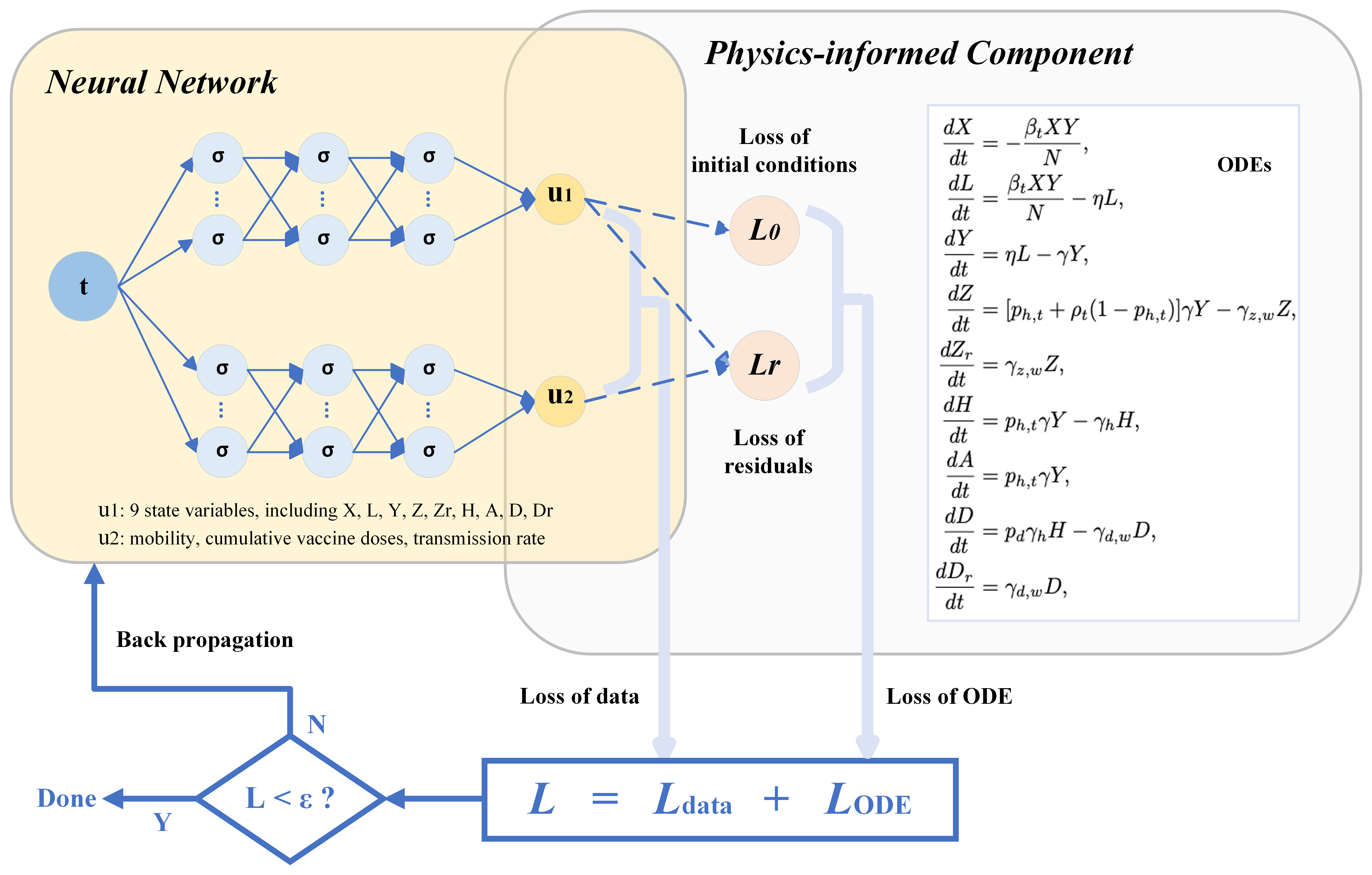
Figure 1: Structure of the proposed PINNs model for infectious disease forecasting. The PINNs model includes two sub-networks: one is designed for predicting the state variables in the compartmental model, while the other provides predictions for the time-dependent model parameters. The predictions of the two sub-networks u1 and u2 are directly used to compute the data loss, $L_{data}$, which is a weighted sum of contribution from different state variables. These predictions of neural networks are also plugged into the ODE model for computing the ODE loss $L_{r}$.

Here, we introduce a new disease forecasting model based on PINNs. The compartmental model we used contains nine state variables, as listed in Table 1. In addition to the FNN used in the traditional PINNs model, we employ an additional sub-network to account for mobility, vaccination, and other potential covariates that might affect the transmission rate, a key parameter in the compartment model. To demonstrate the capability of this approach, we evaluate the performance of the model by comparing 1-, 2-, 3- and 4-weeks-ahead forecasts of COVID-19 cases, hospital admissions, and deaths in the state of California using reports of COVID-19, Google’s mobility reports, and vaccination data available each week. We assessed model forecasts using weighted interval score [50], which is a known “proper” score for forecasting. We compared the score of our model with the original compartmental model, a naive baseline forecast, and FNNs trained with data only.

2 Data and Methods

2.1 Data

2.1.1 Input Data

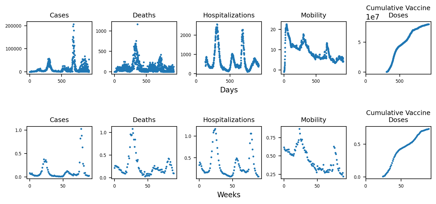
Figure 2: Original dataset (upper panel) and preprocessed (lower panel) dataset used for training and testing the proposed PINNs model.

To facilitate a comparison of our model’s forecasting performance with that of various other models, we used the forecasting targets defined by the COVID-19 Forecast Hub [51, 21], including COVID-19 case and death data sourced from the COVID-19 Data Repository available at https://github.com/CSSEGISandData/COVID-19, which is maintained by the Center for Systems Science and Engineering (CSSE) at Johns Hopkins University, Baltimore, MD, USA (JHU)[52]. Furthermore, we used information on hospital admissions from the COVID-19 Reported Patient Impact and Hospital Capacity by State Timeseries and COVID-19 Reported Patient Impact and Hospital Capacity by State datasets compiled by the US Department of Health & Human Services (HHS) available on healthdata.gov. Access to these datasets was facilitated through the Delphi Epidata API, as detailed by Reinhart et al. [53]. For our analysis, the time series of hospitalizations is the sum of the fields labeled previous_day_admission_adult_covid_confirmed and previous_day_admission_pediatric_covid_confirmed in the tables provided by HHS.

We used data on mobility and susceptibility as they relate to transmission rate, a significant time-dependent factor for epidemiology forecasting. In particular, mobility can be measured by the amount of time individuals spend in residential areas, as quantified in Google’s community mobility reports [54]. The details of the calculation of our mobility covariate are as follows. For a given forecast date, we obtained the latest snapshot of Google’s Global_Mobility_Report.csv file on http://web.archive.org that was made before the beginning forecast date in the UTC time zone.

Susceptibility is related to the number of vaccine doses administered in a state. The modeling assumption is that the average susceptibility of previously uninfected persons declines with the number of doses administered. We model an effect on average susceptibility rather than the number of susceptibles because a single dose of a COVID-19 vaccine generally does not fully immunize an individual. We sourced our time series of the number of doses administered from the Git repository at www.github.com/govex/COVID-19, which was created by Johns Hopkins University. These data came from either the states’ public dashboards or the Centers for Disease Control and Prevention Vaccine Tracker. Since the reported numbers are cumulative, the creators of this dataset used the larger values from those two data sources each day as the most up-to-date value. To obtain a covariate free of missing values, we assumed that all values before the first reported value were zero. Missing values within the time series were imputed with linear interpolation.

2.1.2 Data preprocessing

The time series of cases, deaths, hospitalizations, mobility, and cumulative vaccine doses were provided at a daily resolution, but our prediction targets are weekly totals for cases, deaths, and hospitalizations. To be consistent with the targets, we preprocessed these data, including cases, deaths, hospitalizations, mobility, and cumulative vaccine doses, by calculating a 7-day average and transforming the daily dataset to a weekly time series. This smoothing strategy also reduces fluctuations in the original dataset. The hospital admissions time series is different from other datasets as it is recorded later than the cases and deaths time series, and it did not become available until July 2020. At the beginning of the hospital admissions time series, a misleading trend also arose because the number of hospitals providing data was increasing. To align the targets, we discarded data from the first 20 weeks. Additionally, near the end of the time series, there is a small and incomplete peak after two major peaks. We choose to model only the two major peaks and discard the small incomplete peak after week 110. The two major peaks are driven by different virus variants (Beta and Delta) with changing transmission rates, which is sufficient to evaluate the performance of our model.

Fig. 2 shows the original (upper panel) and preprocessed (lower panel) data. In addition, since the time series differ greatly in scale, we perform linear scaling to transform them to a similar scale around 0 to 1, as shown in the lower panel of Fig. 2.

2.2 Physics-informed neural networks

Name	Definition
$X$	Uninfected and susceptible individuals
$L$	Individuals with latent infections who are not yet infectious
$Y$	Individuals who are infectious
$Z$	Individuals who have been diagnosed and will be reported as cases but have not yet been reported
$Z_{r}$	This compartment keeps track of the number of cases reported each day
$H$	Individuals who have been hospitalized
$A$	Individuals who are new hospital admissions
$D$	Individuals who have died from the infection but whose death has not yet been reported
$D_{r}$	The number of newly reported deaths each week

Table 1: State variables in the employed compartment model by O’Dea and Drake [21].

Physics-informed neural networks (PINNs), which integrate traditional compartment models and data using NNs, have emerged as one of the most influential models in scientific machine learning. We integrate the epidemiology model proposed in [21], which is a compartmental model for COVID-19 with time-dependent parameters, into the proposed PINNs model. The ODE system contains nine equations with nine state variables as well as 11 parameters. The definitions for each state variable are shown in Table 1. Three of the nine state variables ($Z_{r}$, $D_{r}$ and $A$) are observable and were used as targets for training and evaluation. The other six state variables are unobservable and implicit.

Name	Definition	Value
$\beta_{t}$	Transmission rate	estimated
$N$	Population size	39512223
$\eta$	Incubation rate	0.25
$\gamma$	Removal rate	0.25
$\gamma_{d,w}$	Rate of reporting deaths on day of week w	0.1
$\gamma_{z,w}$	Rate of reporting cases on day of week w	1
$\gamma_{h}$	Rate of exit from hospital	0.1
$p_{h,t}$	Probability of an infection leading to hospitalization	estimated
$p_{d}$	Probability of a hospitalization leading to death	estimated
$\rho_{t}$	Probability of a removal on day $t$ being reported as a case	0.5

Table 2: Model parameters used in the compartment model by O’Dea and Drake [21].

The ODEs are summarized in the physics-informed part in Fig. 1. The definitions and values for each parameter are shown in Table 2. For comparison, we generally adopt the model parameters following the work of [21]: 7 are considered to be known and constant, while three parameters were estimated. Transmission rate $\beta_{t}$ is considered a critical time-dependent parameter and was predicted by a sub-network as shown in Fig. 1. The parameters $p_{h}$ and $p_{d}$ are assumed to be constant and were estimated during model training.

As depicted in Fig. 1, the NNs in PINNs consist of two sub-networks. Both of the sub-networks take time as inputs. Each sub-network consists of three hidden layers with 50 neurons in each layer. One sub-network outputs nine state variables corresponding to the nine variables in the ODE system. This sub-network aims to fit three targets, namely cases, deaths, and hospitalizations, and all nine outputs were used to calculate the loss on the ODEs. The second sub-network outputs three variables, namely mobility, cumulative vaccine doses, and transmission rate. This sub-network aims to fit the mobility data and cumulative vaccine doses time series and outputs transmission rate, which was also used to calculate the loss on the ODEs.

The constraint of the compartmental theory was incorporated into the PINNs training process by adding the loss on the ODEs to the loss on the data, i.e. the total loss was given by the weighted sum of data loss and ODE loss:

$$\mathcal{L}(\theta)=w_{data}\mathcal{L}_{data}(\theta)+w_{ODE}\mathcal{L}_{ODE}(\theta)$$ (1)

where $\theta$ denotes the PINNs parameters, $\mathcal{L}_{data}$ denotes data loss, $\mathcal{L}_{ODE}$ denotes ODE loss, $w_{data}$ denotes the weight for data loss, and $w_{ODE}$ denotes the weight for ODE loss.

We denote the PINNs as $\bm{y}_{\theta}(\bm{t})$ where $\bm{t}$ denotes input time and $\bm{y}=[y_{1},y_{2},y_{3},y_{4},y_{5}]^{T}$ denotes output with $y_{1}$ to $y_{5}$ representing cases, deaths, hospitalizations, mobility and cumulative vaccine doses respectively. We used the mean squared error (MSE) as the metric for training with the following loss function for data:

$$\mathcal{L}_{data}(\theta)=\frac{1}{N_{data}}\sum_{i=1}^{N_{data}}|\bm{y}_{\theta}(\bm{t}_{i})-\bm{y}_{i}|^{2},$$ (2)

where $N_{data}$ is the number of training data and $\{\bm{t}_{i},\bm{y}_{i}\}$ represents the $i$th data point. Then, we trained the PINNs $\bm{y}_{\theta}$ by minimizing the loss function $\mathcal{L}(\theta)$. The Adam optimizer [55] was used with $1\times 10^{-3}$ learning rate for $100,000$ epochs. The hyperparameters, including the learning rate and the weight coefficients, are manually tuned to optimize the prediction accuracy. We trained and tested on a GPU named NVIDIA GeForce RTX 3090.

ODE loss was defined as the sum of the loss on the initial conditions and the loss on residuals.

$$\mathcal{L}_{ODE}(\theta)=w_{0}\mathcal{L}_{0}(\theta)+w_{r}\mathcal{L}_{r}(\theta)$$ (3)

where $\mathcal{L}_{0}$ denotes initial condition loss, $\mathcal{L}_{r}$ denotes residual loss, $w_{0}$ denotes the weight for initial condition loss, and $w_{r}$ denotes the weight for residual loss.

Initial condition loss $\mathcal{L}_{0}(\theta)$ and residual loss $\mathcal{L}_{r}(\theta)$ were measured by MSE:

$$\mathcal{L}_{0}(\theta)=\frac{1}{N_{0}}\sum_{i=1}^{N_{0}}{|\bm{y}_{\theta}(\bm{t}_{0})-\bm{y_{i}}|^{2}}$$ (4)

$$\mathcal{L}_{r}(\theta)=\frac{1}{N_{ODE}}\sum_{i=1}^{N_{ODE}}{|w_{i}f(t_{i})|^{2}}$$ (5)

where $N_{0}$ denotes the number of initial data, $N_{ODE}$ denotes the number of ODEs, $w_{i}$ denotes the weight for each ODE, and $f(t)$ is defined to be given by the difference between left-hand-side and right-hand-side of ODE; i.e., for the first equation $\frac{dX}{dt}=(-\frac{\beta_{t}XY}{N})$ in the ODE system,

$$f:=\frac{dX}{dt}-(-\frac{\beta_{t}XY}{N})$$ (6)

We trained PINNs using historical data from July 2020 to April 2022. The model was developed with a rolling window approach, allowing continuous predictions for the following 1 to 4 weeks. Initially, we trained PINNs on preprocessed data spanning 1 to 17 weeks and made predictions for weeks 18 to 21. We then shifted the training window by one week, training new PINNs with data from weeks 1 to 18 and predicting for weeks 19 to 22. This process was repeated until we trained PINNs using data from weeks 1 to 89 and predicted for weeks 90 to 93. Consequently, each week from 21 to 90 had been treated as the subsequent 1, 2, 3, and 4 weeks during the rolling window approach.

2.3 Evaluation metrics

We used two metrics to assess predictive performance: mean absolute scaled error (MASE) [56] and weighted interval score (WIS). MASE was calculated by dividing the mean absolute error (MAE) of the model prediction by the MAE of a naive model.

$$MASE=\frac{{MAE_{PINNs}}}{MAE_{naive}}$$ (7)

MAE was calculated as the mean absolute difference between model predictions $\hat{y_{i}}$ and empirical observations $y_{i}$:

$$MAE=\frac{1}{N}{\sum_{i=1}^{N}|\hat{y_{i}}-y_{i}|}$$ (8)

where $N$ is the number of data.

The naive model uses the data from the past weeks as predictions for the following weeks. Specially speaking, when the forecast horizon is 1 week, the naive model uses the data of the past 1 week as the predictions for the following 1 week. When the forecast horizon is 2 weeks, the naive model uses the data of the past 2 weeks as the forecasting of the following 2 weeks. MASE smaller than 1.0 means that our PINNs model predicts more accurately than the naive model. And the lower the MASE, the more accurate the predictions.

The typical use case for infectious disease forecasting requires probabilistic predictions. For error propagation, we assume that the prediction distribution is Gaussian with mean $\mu_{t}$ equal to the point forecast for time $t$ and standard deviation $\sigma$ equal to the standard deviation of all prediction errors, constant across time yielding $\mu_{t}+\sigma\sqrt{2}{erf}^{-1}(2p-1)$ for prediction quantiles at $t$.

To evaluate probabilistic predictions with WIS, we used the ‘interval-scoring’ Python package (https://github.com/adrian-lison/interval-scoring), based on  [50], to calculate WIS, with quantile bins as required by the COVID-19 Forecast Hub, i.e., $\alpha 1=0.02$, $\alpha 2=0.05$, $\alpha 3=0.1$,…,$\alpha 11=0.9$ and quantiles including 0.010, 0.025, 0.050, 0.100, 0.150, 0.200, 0.250, 0.300, 0.350, 0.400, 0.450, 0.500, 0.550, 0.600, 0.650, 0.700, 0.750, 0.800, 0.850, 0.900, 0.950, 0.975, 0.990.

2.4 Ablation study

Compared with traditional neural networks, we employed epidemiology information in the networks by adding a loss of ODE into the overall loss function. To investigate the impact of embedding the epidemiological domain knowledge into the neural network, we also trained a traditional feed-forward neural network (FNN) and compared its performance with our PINNs model. Both PINNs and FNNs were fitted five times with different initial configurations. Predictions were obtained as the mean of the five results.

Compared with traditional mathematical methods, we used an FNN and embedded the compartment model into the FNN. To examine the advantage of PINNs over the compartment model, we compared GISST’s performance with our PINN model. GISST[22] solves the same compartmental model by semi-parametric mathematical methods.

It is noted that early history data may not reflect the dynamics of the current type of virus due to the mutation and even negatively affect future predictions. Thus, we also examined the impact of the size of the training data set on the prediction accuracy. We first trained PINNs with all historical data. We trained PINNs with data from the past few weeks instead of all the historical data and compared their predicted performances. The results are reported in Appendix 5.1.

Finally, we also investigated applying L2 regularization to our model to avoid overfitting. L2 Regularization was achieved by adding a new term, which consists of the sum of the squared values of the network’s hyperparameters, to the original loss function of PINNs during training. The regularization term penalizes certain model parameters and adjusts them to minimize the total loss of the PINNs. We examined the impact of L2 regularization to investigate how this feature impacts the performance of the model. The results are reported in Appendix 5.2.

3 Results

3.1 Point forecasts on the number of cases, deaths, and hospitalizations for the following 1 - 4 weeks

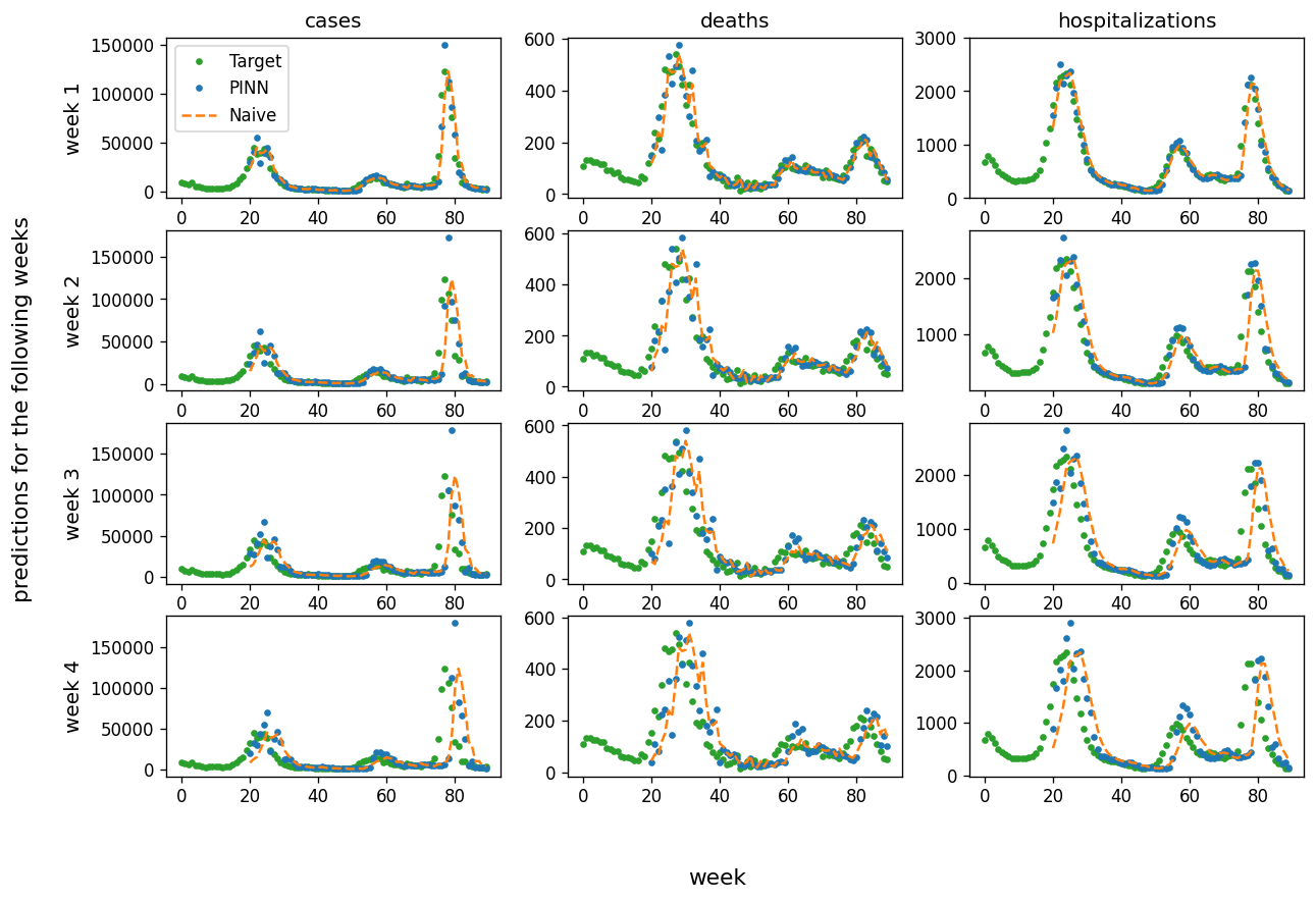
Figure 3: PINNs’ point predictions on the number of cases, deaths, and hospitalizations for the following 1 - 4 weeks.

At each time point $t$, we trained PINNs with historical data from July 2020 to $t$ and made predictions for the following 1-4 weeks. We plotted the predictions in Fig. 3, which demonstrates that PINNs predictions are consistent with the target and more accurate than the naive model for all forecasting horizons from 1 week to 4 weeks. It also shows that one-week-ahead predictions are more accurate than predictions with 2, 3, and 4-week time horizons. As the time horizon for forecasting becomes greater, the predicted values deviate more from the true values, and there are more fluctuations in the curves as well.

Evaluation metrics are reported in Table 3. In the column labeled ’Method’, the name before the dash denotes the approach, while the number is the number denotes the length of forecast horizon. Scores in red denote the model with the lowest score for a given forecast horizon in that column, e.g., PINNs - 1 week denotes PINNs predictions for the following 1 week. We find that PINNs’ MASE scores are all less than 1.0, meaning that PINNs outperform the naive model for all the forecast horizons. Among the three state variables, MASE scores of deaths are higher than the scores of cases and hospitalizations because deaths are associated with larger fluctuations in the original dataset.

Method	MASE			WIS			scaled WIS
	Cases	Deaths	Hosp	Cases	Deaths	Hosp	Cases	Deaths	Hosp
PINN - 1 week	0.75	1.00	0.58	16247	103	250	0.70	1.04	0.57
PINN - 2 week	0.77	0.92	0.62	29570	140	562	0.71	0.96	0.66
PINN - 3 week	0.81	0.86	0.68	43331	174	951	0.76	0.90	0.78
PINN - 4 week	0.85	0.89	0.74	57471	230	1416	0.85	0.94	0.91
NN - 1 week	0.91	1.32	0.65	25152	158	298	1.09	1.60	0.68
NN - 2 week	1.27	1.76	0.79	52761	298	729	1.27	2.04	0.86
NN - 3 week	1.56	1.86	0.89	88920	442	1281	1.57	2.29	1.05
NN - 4 week	1.65	1.84	0.97	118515	558	1885	1.76	2.28	1.22
GISST - 1 week	0.85	0.88	0.91	15346	163	401	0.66	1.65	0.92
GISST - 2 week	0.75	0.64	0.78	26233	185	798	0.63	1.27	0.94
GISST - 3 week	0.71	0.45	0.77	37041	187	1300	0.65	0.97	1.06
GISST - 4 week	0.76	0.34	0.89	58148	181	2159	0.86	0.74	1.39

Table 3: MASE and WIS comparison of different methods for point forecasting and quantile forecasting, respectively. Column Hosp denotes hospitalizations. Scaled WIS is computed by dividing the WIS by the WIS of naive models of the same forecast horizon. Scores in red denote the lowest score of the same forecast horizon in that column.

3.2 Quantile forecasts on the number of cases, deaths, and hospitalizations for the following 1 - 4 weeks

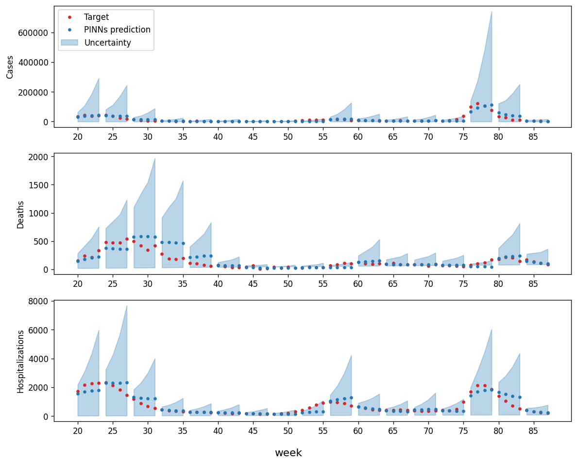
Figure 4: PINNs’ quantile predictions on the number of cases, deaths, and hospitalizations for the following 1 - 4 weeks. The red dots represent the ground truth; the blue points denote the PINNs predictions; the blue region represents the uncertainty. Different polygons cover a four-week prediction interval with 1-, 2-, 3- and 4-week predictions from a time one week prior to the polygon.

Similarly, at each time point $t$, we trained PINNs with historical data from July 2020 to $t$ and made predictions for the following 1-4 weeks. In this case, we plotted the continuous predictions for the following 1-4 weeks as well as the corresponding uncertainty in Fig. 4. For each group of predictions for the following 1-4 weeks, the points (denoting predictions at quantile = 0.5) gradually deviate from the target, and the light blue area (denotes uncertainty) grows larger. The longer the forecast horizons, the lower the accuracy and the larger the uncertainty.

WIS scores are reported in Table 3. Scaled WIS was computed by dividing the WIS by the WIS of naive models of the same forecast horizon. We find that PINNs WIS scores are mostly less than 1.0, which means that PINNs outperform the naive model for all the forecast horizons. The only exception is the quantile predictions by PINNs for the following 1 week.

3.3 Comparison with traditional neural network and traditional mathematical method

We compared our PINNs predictions with results obtained from the traditional neural network model (FNN) without incorporating the compartment model as well as with the results of a mathematical model, named Gaussian infection state space with time dependence (GISST) [21]. As shown in Table 3, both MASE and WIS scores for PINNs are lower than the corresponding FNN scores for each forecast horizon, which demonstrates the absolute advantage of PINNs over traditional neural networks for both point forecasting and quantile forecasting. This is likely due to the regularizing effect of the compartment model. Additionally, PINNs typically outperformed GISST when forecasting hospitalizations, GISST outperformed PINNs for cases, and forecasting performance for deaths depended on whether the evaluation was for point forecasts (GISST superior) or quantile forecasts (PINNs superior). These results demonstrate the important role of epidemiological domain knowledge as a constraint to avoid unreasonable predictions that may arise in purely data-driven modeling.

4 Discussion and Summary

Epidemic forecasting can be generally considered an inverse-forward problem, meaning that we need to first infer the parameters of the model before making a forecast. In many cases, we partially know the mechanisms underlying disease transmission, which is represented by the compartment models in the form of ODEs, but some of the model parameters need to be identified by fitting them to observation data. Once the parameters are estimated, compartment models can be used to predict future disease trends and assess potential shifts induced by changes in public health policies or emerging variants. The main shortcomings of the traditional mathematical models are the limitations due to model misspecification, such as assuming transition rates are fixed, making it difficult to adapt to variants with different transmission rates. On the other hand, data-driven neural network models have emerged as a new tool for tackling complex social problems over the last several years. However, conventional neural network models require a large amount of training and labeled data to ensure good performance, and they also fail to account for domain knowledge. Furthermore, ML models may provide unrealistic predictions in cases of extrapolation as they do not take into account the mechanisms underlying relevant physical processes.

In this work, we employed PINNs to leverage the epidemiological knowledge contained in compartment models together with observed data to improve the accuracy of infectious disease forecasts. Our results have demonstrated that the proposed model possesses several features that may contribute to its superior performance. First, the PINN model utilizes NNs to capture complex and non-linear relationships within infectious disease data because neural networks can represent complex non-linear dynamics. Second, PINN models integrate domain-specific knowledge by incorporating the compartment models into the loss function of the NNs to ensure that the learned model adheres to the fundamental principles and constraints of disease dynamics. In addition, incorporating compartment models could prevent the model from overfitting, which often occurs when training machine learning models with only data.

Additionally, PINNs can be used to estimate key epidemiological parameters, such as transmission rates or recovery rates, directly from the data, thereby enhancing the model’s ability to adapt to changes in the disease dynamics over time. Particularly, PINNs treat these parameters as the output of the neural network such that these parameters can be time-dependent, representing the change of the dynamics of the transmission induced by, i.e., the mutation of the virus. We also show that PINNs can continuously adapt to newly acquired data, allowing the model to continuously improve its forecasting capabilities as more information becomes available during an ongoing outbreak. PINNs can integrate data from various sources, including social, environmental, and demographic factors, providing a holistic approach to infectious disease forecasting.

Recently, several Physics-Informed Neural Network (PINNs) models have been developed for infectious disease forecasting such as COVID-19 [57, 58, 59] and measles [60]. Compared with these models, our proposed model incorporates a more complex compartmental framework with nine state variables into the neural network, presenting a greater challenge for the model to align with the physics described by the ODE system. In particular, our model achieves better metrics, namely Normalized Root Mean Squared Error (NR1 and NR2) and Normal Deviation (ND) as defined in [58], than the Epidemiologically-Informed Neural Networks (EINNs) [58] on predicting the death in COVID-19, the only predicted state variables of EINNs. Additionally, while previous models primarily provide point forecasts, our approach facilitates quantile forecasts, which convey uncertainty and enhance the reliability of predictions.

Notwithstanding its capabilities of dealing with noisy data, the vanilla PINN model is not equipped with built-in mechanisms to assess the uncertainty of model predictions in response to noisy input data. One popular approach for solving regression problems with uncertainty is Gaussian processes regression (GPR). Built upon the Bayesian framework, GPR can quantify uncertainty in the solution of PDEs, but the applications of GPR have been limited to linear problems with small datasets as its computational cost increases substantially with the growing size of the dataset. One possible approach to resolve this challenge is to employ Bayesian PINNs as has been proposed by [37]. These models take advantage of the function of PINNs in solving ill-posed problems, i.e., with under-defined boundary conditions, and the capability of the Bayesian framework to quantify the uncertainty for the solution. Thus, the performance of Bayesian PINNs on infectious disease forecasting needs to be explored in a future study.

In summary, the application of PINNs in infectious disease forecasting offers a synergistic approach that combines the power of data-driven deep learning with the interpretability and constraints provided by underlying epidemiological principles, leading to more accurate, interpretable, and adaptable models for predicting the spread of infectious diseases.

Data Availability

All relevant code and data are available from https://github.com/dpdclub/PINNs-for-Epidemiology-.

Funding

This work was supported by National Institute of Health grants R21HL168507 and NSF SCH Award Number:2406212. High-performance computing resources were provided by the Center for Computation and Visualization at Brown University and The Georgia Advanced Computing Resource Center (GACRC) at the University of Georgia.

5 Appendices

5.1 Impact of training data length

Figure 5: MASE for the predictions of PINNs models on cases, deaths, and hospitalizations when trained with varied lengths of historical data ranging from 4 weeks to 24 weeks.

We trained PINNs using data from the most recent 4, 8, 12, 16, 20, and 24 weeks and evaluated their predicting performances on weeks 48 to 110. The result is shown in Fig. 5. Each subplot shows the MASE scores of predictions on cases, deaths, and hospitalizations for the following 1, 2, 3, and 4 weeks by using different lengths of training data ranging from 4 to 24 weeks. For all the three targets, the overall trend of MASE values is that as the training data length becomes longer, MASE gradually falls and then becomes stable. When we only use recent data from 4 or 8 weeks, it seems the data is not enough to capture the disease dynamics. When we use data from the past 12 or 16 weeks, it could present a comparable accuracy compared with PINNs using all the historical data. We also note that when the training data keeps increasing to the recent 20 or 24 weeks’ data, the accuracy of the performance doesn’t make significant further improvement, which is likely that these training data span nearly half a year, and thus they are not closely related to current epidemiology trends and don’t have a significant contribution to predictions.

5.2 Impact of L2 regularization

We further show that without L2 regularization, the model accuracy drops significantly. Removing the L2 regularization results in average decreases of 22.48% in cases, 9.16% in deaths, and 42.54% in hospitalizations for the following 1-4 weeks. This result suggests that L2 regularization can still be beneficial to model predictions in the PINNs model.

References

- [1] Farida B Ahmad, Jodi A Cisewski, and Robert N Anderson. Provisional mortality data—united states, 2021. Morbidity and Mortality Weekly Report, 71(17):597, 2022.
- [2] David M Morens, Gregory K Folkers, and Anthony S Fauci. The challenge of emerging and re-emerging infectious diseases. Nature, 430(6996):242–249, 2004.
- [3] Colin J Carlson, Gregory F Albery, Cory Merow, Christopher H Trisos, Casey M Zipfel, Evan A Eskew, Kevin J Olival, Noam Ross, and Shweta Bansal. Climate change increases cross-species viral transmission risk. Nature, 607(7919):555–562, 2022.
- [4] Matthew Biggerstaff, Rachel B Slayton, Michael A Johansson, and Jay C Butler. Improving pandemic response: employing mathematical modeling to confront coronavirus disease 2019. Clinical Infectious Diseases, 74(5):913–917, 2022.
- [5] Chelsea S Lutz, Mimi P Huynh, Monica Schroeder, Sophia Anyatonwu, F Scott Dahlgren, Gregory Danyluk, Danielle Fernandez, Sharon K Greene, Nodar Kipshidze, Leann Liu, et al. Applying infectious disease forecasting to public health: a path forward using influenza forecasting examples. BMC Public Health, 19(1):1–12, 2019.
- [6] R M Anderson and R M May. Infectious Diseases of Humans. Oxford University Press. Oxford University Press, 1991.
- [7] M J Keeling and P Rohani. Modelling Infectious Diseases: In Humans and Animals. Princeton University Press. Princeton University Press, 2008.
- [8] Fred Brauer. Compartmental models in epidemiology. Mathematical epidemiology, pages 19–79, 2008.
- [9] Fred Brauer, Carlos Castillo-Chavez, Zhilan Feng, et al. Mathematical models in epidemiology, volume 32. Springer, 2019.
- [10] Maia Martcheva. An introduction to mathematical epidemiology, volume 61. Springer, 2015.
- [11] Amit Huppert and Guy Katriel. Mathematical modelling and prediction in infectious disease epidemiology. Clinical microbiology and infection, 19(11):999–1005, 2013.
- [12] Helen J Wearing, Pejman Rohani, and Matt J Keeling. Appropriate Models for the Management of Infectious Diseases. PLoS Medicine, 2(7):e174, 2005.
- [13] Gemma Massonis, Julio R Banga, and Alejandro F Villaverde. Structural identifiability and observability of compartmental models of the covid-19 pandemic. Annual reviews in control, 51:441–459, 2021.
- [14] Toheeb A Biala and AQM Khaliq. A fractional-order compartmental model for the spread of the covid-19 pandemic. Communications in Nonlinear Science and Numerical Simulation, 98:105764, 2021.
- [15] Faïçal Ndaïrou, Iván Area, Juan J Nieto, and Delfim FM Torres. Mathematical modeling of covid-19 transmission dynamics with a case study of wuhan. Chaos, Solitons & Fractals, 135:109846, 2020.
- [16] Anas Abou-Ismail. Compartmental models of the covid-19 pandemic for physicians and physician-scientists. SN comprehensive clinical medicine, 2(7):852–858, 2020.
- [17] Cristiane M Batistela, Diego PF Correa, Átila M Bueno, and José Roberto C Piqueira. Sirsi compartmental model for covid-19 pandemic with immunity loss. Chaos, Solitons & Fractals, 142:110388, 2021.
- [18] Takashi Odagaki. New compartment model for covid-19. Scientific Reports, 13(1):5409, 2023.
- [19] Matthieu Domenech de Cellès, Felicia M. G. Magpantay, Aaron A. King, and Pejman Rohani. The impact of past vaccination coverage and immunity on pertussis resurgence. Science Translational Medicine, 10(434):eaaj1748, 03 2018.
- [20] Adam J Kucharski, Anton Camacho, Stefan Flasche, Rebecca E Glover, W John Edmunds, and Sebastian Funk. Measuring the impact of Ebola control measures in Sierra Leone. Proceedings of the National Academy of Sciences of the United States of America, 112(46):14366 – 14371, 11 2015.
- [21] Eamon B O’Dea and John M Drake. A semi-parametric, state-space compartmental model with time-dependent parameters for forecasting covid-19 cases, hospitalizations and deaths. Journal of the Royal Society Interface, 19(187):20210702, 2022.
- [22] John M Drake, Andreas Handel, Éric Marty, Eamon B O’Dea, Tierney O’Sullivan, Giovanni Righi, and Andrew T Tredennick. A data-driven semi-parametric model of sars-cov-2 transmission in the united states. PLOS Computational Biology, 19(11):e1011610, 2023.
- [23] Graham C Gibson, Nicholas G Reich, and Daniel Sheldon. Real-time mechanistic bayesian forecasts of covid-19 mortality. medRxiv, 2020.
- [24] Yuexin Wu, Yiming Yang, Hiroshi Nishiura, and Masaya Saitoh. Deep learning for epidemiological predictions. In The 41st International ACM SIGIR Conference on Research & Development in Information Retrieval, pages 1085–1088, 2018.
- [25] Yixiang Deng and He Li. Deep learning for few-shot white blood cell image classification and feature learning. Computer Methods in Biomechanics and Biomedical Engineering: Imaging & Visualization, 11(6):2081–2091, 2023.
- [26] Lu Lu, Ying Qian, Yihang Dong, Han Su, Yunxin Deng, Qiang Zeng, and He Li. A systematic study of the performance of machine learning models on analyzing the association between semen quality and environmental pollutants. Frontiers in Physics, 11:1259273, 2023.
- [27] Qi Gao, Hongtao Lin, Jianghong Qian, Xingli Liu, Shengze Cai, He Li, Hongguang Fan, and Zhe Zheng. A deep learning model for efficient end-to-end stratification of thrombotic risk in left atrial appendage. Engineering Applications of Artificial Intelligence, 126:107187, 2023.
- [28] Vishnu Vytla, Sravanth Kumar Ramakuri, Anudeep Peddi, K Kalyan Srinivas, and N Nithish Ragav. Mathematical models for predicting covid-19 pandemic: a review. In Journal of Physics: Conference Series, volume 1797, page 012009. IOP Publishing, 2021.
- [29] George Em Karniadakis, Ioannis G. Kevrekidis, Lu Lu, Paris Perdikaris, Sifan Wang, and Liu Yang. Physics-informed machine learning. Nature Reviews Physics, 3(6):422–440, 2021.
- [30] Maziar Raissi, Alireza Yazdani, and George Em Karniadakis. Hidden fluid mechanics: Learning velocity and pressure fields from flow visualizations. Science, 367(6481):1026–1030, 2020.
- [31] Lu Lu, Ming Dao, Punit Kumar, Upadrasta Ramamurty, George Em Karniadakis, and Subra Suresh. Extraction of mechanical properties of materials through deep learning from instrumented indentation. Proceedings of the National Academy of Sciences, 117(13):7052–7062, 2020.
- [32] Zongren Zou and George Em Karniadakis. L-hydra: Multi-head physics-informed neural networks. arXiv preprint arXiv:2301.02152, 2023.
- [33] Zongren Zou, Xuhui Meng, and George Em Karniadakis. Correcting model misspecification in physics-informed neural networks (pinns). arXiv preprint arXiv:2310.10776, 2023.
- [34] Zhen Zhang, Zongren Zou, Ellen Kuhl, and George Em Karniadakis. Discovering a reaction-diffusion model for alzheimer’s disease by combining pinns with symbolic regression. arXiv preprint arXiv:2307.08107, 2023.
- [35] Zongren Zou, Xuhui Meng, and George Em Karniadakis. Uncertainty quantification for noisy inputs-outputs in physics-informed neural networks and neural operators. arXiv preprint arXiv:2311.11262, 2023.
- [36] Zongren Zou, Xuhui Meng, Apostolos F Psaros, and George Em Karniadakis. Neuraluq: A comprehensive library for uncertainty quantification in neural differential equations and operators. arXiv preprint arXiv:2208.11866, 2022.
- [37] Liu Yang, Xuhui Meng, and George Em Karniadakis. B-pinns: Bayesian physics-informed neural networks for forward and inverse PDE problems with noisy data. Journal of Computational Physics, 425:109913, 2021.
- [38] Xuhui Meng, Zhen Li, Dongkun Zhang, and George Em Karniadakis. Ppinn: Parareal physics-informed neural network for time-dependent pdes. Computer Methods in Applied Mechanics and Engineering, 370:113250, 2020.
- [39] Jeremy Yu, Lu Lu, Xuhui Meng, and George Em Karniadakis. Gradient-enhanced physics-informed neural networks for forward and inverse pde problems. Computer Methods in Applied Mechanics and Engineering, 393:114823, 2022.
- [40] Qin Lou, Xuhui Meng, and George Em Karniadakis. Physics-informed neural networks for solving forward and inverse flow problems via the boltzmann-bgk formulation. Journal of Computational Physics, 447:110676, 2021.
- [41] Lu Lu, Xuhui Meng, Zhiping Mao, and George Em Karniadakis. Deepxde: A deep learning library for solving differential equations. SIAM review, 63(1):208–228, 2021.
- [42] Maziar Raissi, Paris Perdikaris, and George E Karniadakis. Physics-informed neural networks: A deep learning framework for solving forward and inverse problems involving nonlinear partial differential equations. Journal of Computational Physics, 378:686–707, 2019.
- [43] Qian Zhang, Konstantina Sampani, Mengjia Xu, Shengze Cai, Yixiang Deng, He Li, Jennifer K Sun, and George Em Karniadakis. Aoslo-net: a deep learning-based method for automatic segmentation of retinal microaneurysms from adaptive optics scanning laser ophthalmoscopy images. Translational Vision Science & Technology, 11(8):7–7, 2022.
- [44] Qijing Chen, Qi Ye, Weiqi Zhang, He Li, and Xiaoning Zheng. Tgm-nets: A deep learning framework for enhanced forecasting of tumor growth by integrating imaging and modeling. Engineering Applications of Artificial Intelligence, 126:106867, 2023.
- [45] Mitchell Daneker, Shengze Cai, Ying Qian, Eric Myzelev, Arsh Kumbhat, He Li, and Lu Lu. Transfer learning on physics-informed neural networks for tracking the hemodynamics in the evolving false lumen of dissected aorta. Nexus, 1(2), 2024.
- [46] Qijing Chen, He Li, and Xiaoning Zheng. A deep neural network for operator learning enhanced by attention and gating mechanisms for long-time forecasting of tumor growth. Engineering with Computers, pages 1–111, 2024.
- [47] Ying Qian, Ge Zhu, Zhen Zhang, Susree Modepalli, Yihao Zheng, Xiaoning Zheng, Galit Frydman, and He Li. Coagulo-net: Enhancing the mathematical modeling of blood coagulation using physics-informed neural networks. Neural Networks, page 106732, 2024.
- [48] Shengze Cai, He Li, Fuyin Zheng, Fang Kong, Ming Dao, George Em Karniadakis, and Subra Suresh. Artificial intelligence velocimetry and microaneurysm-on-a-chip for three-dimensional analysis of blood flow in physiology and disease. Proceedings of the National Academy of Sciences, 118(13):e2100697118, 2021.
- [49] Kevin Linka, Amelie Schäfer, Xuhui Meng, Zongren Zou, George Em Karniadakis, and Ellen Kuhl. Bayesian physics informed neural networks for real-world nonlinear dynamical systems. Computer Methods in Applied Mechanics and Engineering, 402:115346, 2022.
- [50] Johannes Bracher, Evan L Ray, Tilmann Gneiting, and Nicholas G Reich. Evaluating epidemic forecasts in an interval format. PLoS computational biology, 17(2):e1008618, 2021.
- [51] Evan L Ray, Nutcha Wattanachit, Jarad Niemi, Abdul Hannan Kanji, Katie House, Estee Y Cramer, Johannes Bracher, Andrew Zheng, Teresa K Yamana, Xinyue Xiong, et al. Ensemble forecasts of coronavirus disease 2019 (covid-19) in the us. MedRXiv, pages 2020–08, 2020.
- [52] Ensheng Dong, Hongru Du, and Lauren Gardner. An interactive web-based dashboard to track covid-19 in real time. The Lancet infectious diseases, 20(5):533–534, 2020.
- [53] Alex Reinhart, Logan Brooks, Maria Jahja, Aaron Rumack, Jingjing Tang, Sumit Agrawal, Wael Al Saeed, Taylor Arnold, Amartya Basu, Jacob Bien, et al. An open repository of real-time covid-19 indicators. Proceedings of the National Academy of Sciences, 118(51):e2111452118, 2021.
- [54] Google LLC. Google covid-19 community mobility reports. See https://www.google.com/ covid19/mobility/, 2020.
- [55] Diederik P Kingma and Jimmy Ba. Adam: A method for stochastic optimization. arXiv preprint arXiv:1412.6980, 2014.
- [56] Rob J Hyndman and Anne B Koehler. Another look at measures of forecast accuracy. International journal of forecasting, 22(4):679–688, 2006.
- [57] Sarah Berkhahn and Matthias Ehrhardt. A physics-informed neural network to model covid-19 infection and hospitalization scenarios. Advances in continuous and discrete models, 2022(1):61, 2022.
- [58] Alexander Rodríguez, Jiaming Cui, Naren Ramakrishnan, Bijaya Adhikari, and B Aditya Prakash. Einns: epidemiologically-informed neural networks. In Proceedings of the AAAI conference on artificial intelligence, volume 37, pages 14453–14460, 2023.
- [59] Georgios D Barmparis and Giorgos P Tsironis. Physics-informed machine learning for the covid-19 pandemic: Adherence to social distancing and short-term predictions for eight countries. Quantitative Biology, 10(2):139–149, 2022.
- [60] Wyatt Madden, Wei Jin, Ben Lopman, Andreas Zufle, Benjamin D Dalziel, Jessica Metcalf, Bryan D Grenfell, and Max SY Lau. Neural networks for endemic measles dynamics: comparative analysis and integration with mechanistic models. medRxiv, pages 2024–05, 2024.