Cosmology from UNIONS weak lensing profiles of galaxy clusters

Abstract

Cosmological information is encoded in the structure of galaxy clusters. In Universes with less matter and larger initial density perturbations, clusters form earlier and have more time to accrete material, leading to a more extended infall region. Thus, measuring the mean mass distribution in the infall region provides a novel cosmological test. The infall region is largely insensitive to baryonic physics, and provides a cleaner structural test than other measures of cluster assembly time such as concentration. We consider cluster samples from three publicly available galaxy cluster catalogues: the Spectroscopic Identification of eROSITA Sources (SPIDERS) catalogue, the X-ray and Sunyaev-Zeldovich effect selected clusters in the meta-catalogue M2C, and clusters identified in the Dark Energy Spectroscopic Instrument (DESI) Legacy Imaging Survey. Using a preliminary shape catalogue from the Ultraviolet Near Infrared Optical Northern Survey (UNIONS), we derive excess surface mass density profiles for each sample. We then compare the mean profile for the DESI Legacy sample, which is the most complete, to predictions from a suite of simulations covering a range of $\Omega_{\rm m}$ and $\sigma_{8}$, obtaining constraints of $\Omega_{\rm m}=0.29\pm 0.05$ and $\sigma_{8}=0.80\pm 0.04$. We also measure mean (comoving) splashback radii for SPIDERS, M2C and DESI Legacy Imaging Survey clusters of $1.59^{+0.16}_{-0.13}\,$cMpc$/h$, $1.30^{+0.25}_{-0.13}\,$cMpc$/h$ and $1.45\pm 0.11\,$cMpc$/h$ respectively. Performing this analysis with the final UNIONS shape catalogue and the full sample of spectroscopically observed clusters in DESI, we can expect to improve on the best current constraints from cluster abundance studies by a factor of $2$ or more.

1 Introduction

Galaxy clusters, the most massive gravitationally bound structures in the Universe, are a versatile probe of fundamental physics. Their inner mass profile has been extensively studied as a test of cosmology (e.g. Dolag et al., 2004; Balmès et al., 2014), but uncertain modelling of baryonic physics is a major limitation. This is particularly significant in the centre of a cluster where powerful but poorly understood AGN feedback mechanisms have a strong impact on the matter distribution (e.g. van Daalen et al., 2011). This motivates exploring similar structural tests using the outer regions of clusters. Matter in and around a dark matter halo can be separated into two broad categories: orbiting or infalling (Fukushige & Makino, 2001). Orbiting material is gravitationally bound to the halo, and largely lies inside the virial radius. The infall region is the zone where the orbiting component is subdominant—most of the material is either falling in for the first time, or is backsplashed (Gill et al., 2005), that is approaching or passing through the first apocentre of its orbit after infall. While they currently reside beyond the cluster radius, backsplashed galaxies have previously passed through the cluster centre, and thus have experienced strong environmental effects such as ram-pressure stripping and tidal heating. The infall region is typically 1–5 Mpc from the cluster centre and its upper bound is the turnaround radius, where the expansion of the Universe overcomes the gravitational attraction of the halo. This region is outside the influence of significant baryonic feedback effects (Haggar et al., 2021; O’Neil et al., 2021; Towler et al., 2024; Haggar et al., 2024), so the matter distribution should reflect the assembly history of the cluster. Furthermore, while the difficulty of locating the true cluster centre in observations hampers efforts to use the inner profile, mis-centering has been found to produce differences below the level of the measurement uncertainty in the infall region (More et al., 2016; Baxter et al., 2017; Zürcher & More, 2019). Thus, the infall region provides an interesting environment in which to test for cosmological effects.

There has also been recent theoretical interest in the infall region, as its features may provide a more physical definition of the halo boundary. Classical modelling of the matter distribution around clusters separates halos (the ‘1-halo’ component of the galaxy clustering signal) from their environment (the ‘2-halo’ component) around the virial radius, usually defined by a mean density contrast relative to the background or critical density. Galaxy clusters accrete continuously from their environment, however, and some material beyond the virial radius can have been accreted previously; a more informative halo boundary would extend into the infall region, reflecting this ongoing accretion. Several definitions for this extended halo boundary have been proposed (Diemer & Kravtsov, 2014; Tomooka et al., 2020; García et al., 2021; Fong & Han, 2021), the most notable being the splashback radius $r_{\rm sp}$. This is the radius where infalling material accumulates after it has reached the apocenter of its first orbit, and is sensitive to the net accretion rate over one previous dynamical time (Shin & Diemer, 2023).

Haggar et al. (2024) investigated the cosmological dependence of $r_{\rm sp}$, and found its variation with $\Omega_{\rm m}$ and $\sigma_{8}$, the matter density fraction and initial amplitude of density perturbations, is nearly orthogonal to $S_{8}=\sigma_{8}\sqrt{\Omega_{\rm m}/0.3}$, the parameter best constrained by low-redshift tests of the matter distribution such as cosmic shear or cluster abundance. This cosmological dependence of $r_{\rm sp}$ comes from its relation to cluster assembly times. In cosmologies with low $\Omega_{\rm m}$ and high $\sigma_{8}$, clusters form earlier (Amoura et al., 2021) and have more time to become dynamically relaxed. They provide a deeper potential well for material accreted over the last dynamical time, and thus produce a larger splashback radius and a more extended infall region by late times. The converse is true in cosmologies with high $\Omega_{\rm m}$ and low $\sigma_{8}$. Given the parameter dependence of cluster formation time is almost orthogonal to that of abundance (Amoura et al., 2021), observing the infall region could be a highly complementary probe of cosmology to existing low-redshift tests. Mpetha et al. (2024) investigated the prospects for using weak lensing profiles of galaxy clusters to constrain $\Omega_{\rm m}$ and $\sigma_{8}$ for two weak lensing surveys, Euclid Wide (Euclid Collaboration et al., 2022) and the Ultraviolet Near Infrared Optical Northern Survey (UNIONS) (Gwyn et al. 2025, in preparation). In particular, they developed a new test based on the amplitude of the shear in the infall region, showing that for the full UNIONS lensing survey, it should produce constraints competitive with those from cluster abundance.

In this work we will conduct the first attempt at such an analysis, comparing the weak lensing profiles of galaxy clusters to a suite of dark matter simulations using different combinations of $\Omega_{\rm m}$ and $\sigma_{8}$. We make several improvements to the method presented in Mpetha et al. (2024): including mis-centering in the fitting of weak lensing profiles, performing a Monte Carlo sampling over the fit parameter space, and adding realistic scatter to the masses of simulated halos to reproduce observational selection effects. We explore the challenges of this method, and forecast its potential for present and forthcoming surveys, such as UNIONS combined with a spectroscopic galaxy cluster catalogue of the Dark Energy Spectroscopic Instrument (DESI) survey.

The outline of the paper is as follows. In Section 2, we describe the data products used in this work, including three publicly available cluster catalogues and a weak lensing shape catalogue, that will be combined to construct cluster lensing profiles. Section 3 describes the dark-matter-only cosmological simulation suite we use to generate simulated cluster lensing profiles that will be compared to the observations. Section 4 outlines the main steps in the method, including how excess surface mass density profiles, $\Delta\Sigma(R)$, are determined from the cluster and shape catalogues, how these profiles are compared to the simulation profiles, and finally how profiles are fitted to extract specific features of the infall region, such as the splashback radius $r_{\rm sp}$. Section 5.1 presents cosmological constraints derived from the amplitude of the observed $\Delta\Sigma(R)$ in the most complete cluster sample used in this work. In Section 5.2 we then fit the observed $\Delta\Sigma(R)$ profiles of each sample using a theoretical model of the infall region, determining mean splashback radii for each cluster sample. In Section 5.3 we discuss how these fits provide an additional route to constraining cosmological parameters. We discuss our results in Section 6, and conclude in Section 7.

Throughout this work quantities are scaled by $h^{-1}$, where $h$ is the dimensionless Hubble parameter and its value is fixed at $h=0.7$. The Hubble constant at present is $H_{0}=100\,h\,$km s${}^{-1}\,$Mpc^-1. We use various values of $\Omega_{\rm m}$ (as indicated) when computing profiles, such that we can accurately compare observed profiles to profiles in simulations with a chosen $\Omega_{\rm m}$. A prefix of c, for example in cMpc$/h$ denotes a comoving unit, and log is log₁₀, while ln indicates log_e.

2 Data

For the galaxy cluster lensing profiles, we use the weak lensing shape catalogue from the UNIONS survey Guinot et al. (2022); Li et al. (2024); Guerrini et al. (2024), and publicly available lens catalogues from the DESI Legacy Imaging Survey (DLIS) (Wen & Han, 2024), the Spectroscopic Identification of eROSITA Sources (SPIDERS) (Kirkpatrick et al., 2021), and the M2C cluster catalogue. These are described in the following sections. The final cluster samples adopted, and the matched samples selected from the simulations, are summarised in Table 1. Normalised mass and redshift distributions, and a mass-redshift scatter plot, are shown in Fig. 1.

Catalogue	$N$	$\langle z\rangle$	log($\langle M_{200{\rm c}}\rangle)$	$\langle r_{200{\rm c}}\rangle$	log($\langle M_{200{\rm m}}\rangle)$	$\langle r_{200{\rm m}}\rangle$	$\nu_{200{\rm m}}$
			$M_{\odot}/h$	cMpc$/h$	$M_{\odot}/h$	cMpc$/h$
M2C	$392$	$0.234$	$14.52$	$1.28$	$14.63$	$1.83$	$2.93$
DLIS	$16,\!162$	$0.348$	$14.21$	$1.06$	$14.31$	$1.43$	$2.60$
DLIS high	$7,\!343$	$0.346$	$14.33$	$1.16$	$14.42$	$1.56$	$2.76$
SPIDERS	$1,\!241$	$0.274$	$14.48$	$1.27$	$14.59$	$1.78$	$2.92$
Sim	$3,\!888-71,\!613$	$0.204$	$14.20-14.33$	$0.99-1.10$	$14.32-14.45$	$1.45-1.60$	$2.43-2.61$

Table 1: For the observed samples, $N$ is number in the UNIONS footprint. $\Omega_{\rm m}=0.3$, $\sigma_{8}=0.8$ is assumed to convert to $M_{200{\rm m}}$ and the peak height $\nu_{200{\rm m}}$. Radii are given in comoving units. The DLIS high sample uses a larger mass limit. For the simulation halo samples, we give the minimum and maximum value from the full suite.

Figure 1: Left: Mass distributions of the three cluster catalogues used in this work. M2C and SPIDERS clusters have masses calibrated from an X-ray luminosity – mass relationship, and in DLIS a total stellar mass-cluster mass relationship is used. For plotting purposes only, $M_{500{\rm c}}$ values in DLIS have been converted to $M_{200{\rm c}}$ using a fiducial cosmology ($\Omega_{\rm m}=0.3$, $\sigma_{8}=0.8$). Also shown are all the mass distributions of dark matter halos with $0.1<z<0.3$ in $19$ cosmological simulations with different values of $\Omega_{\rm m}$ and $\sigma_{8}$, where darker line colours are simulations with larger values of $S_{8}$. Middle: Redshift distributions of clusters. The redshift of halos in the simulations are taken from 17 snapshots between $z=0.1$ and $z=0.3$, indicated by the grey band. The difference in the redshift distribution explains the large discrepancy in the HMF in the left panel. Right: The mass-redshift distribution, which illustrates the selection biases in the SPIDERS and M2C catalogues.

2.1 UNIONS shape catalogue

The Ultraviolet Near Infrared Optical Northern Survey (UNIONS; Gwyn et al. 2025, in preparation) is a collaboration of wide field imaging surveys of the northern hemisphere. UNIONS consists of the Canada-France Imaging Survey (CFIS), conducted at the 3.6-meter CFHT on Maunakea, members of the Pan-STARRS team, and the Wide Imaging with Subaru HyperSuprime-Cam of the Euclid Sky (WISHES) team. CFHT/CFIS is obtaining deep u and r bands; Pan-STARRS is obtaining deep i and moderate-deep z band imaging, and Subaru is obtaining deep z-band imaging through WISHES and g-band imaging through the Waterloo-Hawaii IfA g-band Survey (WHIGS). These independent efforts are directed, in part, to securing optical imaging to complement the Euclid space mission Euclid Collaboration et al. (2024), although UNIONS is a separate collaboration aimed at maximizing the science return of these large and deep surveys of the northern skies.

The shape catalogue used in this work was created using the ShapePipe software (Farrens et al., 2022). An earlier version of the UNIONS ShapePipe catalogue is described in Guinot et al. (2022), and the first use of the version adopted in this work, ShapePipe v1.3, is in Li et al. (2024). There are several improvements in ShapePipe v1.3, including replacing PSFEx (Bertin, 2011) with the Multi-CCD PSF model (Liaudat et al., 2020) and reducing contamination by artefacts. ShapePipe v1.3 contains nearly $98\,$million sources over $\sim\!3,\!200\,$deg², giving a number density of $8.5\,$arcmin^-2. The shapes of source galaxies are measured with the ShapePipe package on $r$-band images taken by MegaCam on CFHT.

Guerrini et al. (2024) show first systematics diagnostics for ShapePipe v1.3 and introduce methodologies that will be used in future works to validate the galaxy catalogues used for cosmic shear analysis. In ShapePipe v1.3, there is no estimate for the multiplicative shear measurement bias, however this will be subdominant to other sources of uncertainty and can be safely neglected for our analysis. The sources do not have photometric redshifts currently, but an effective redshift distribution $n(z)$ has been constructed using Self Organising Maps (SOMs) (Wright et al., 2020). UNIONS galaxies in the CFHTLenS (Heymans et al., 2012) field W3 are chosen as a representative subset in order to utilise the colour information of the ugriz photometry from CFHTLenS (Hildebrandt et al., 2012). The SOM $n(z)$ for these galaxies is calibrated with the colours of  66,000 galaxies from the deep spectroscopic surveys DEEP2 (Newman et al., 2013), VVDS (Le Fèvre et al., 2005), and VIPERS (Scodeggio et al., 2018) as reference samples. This $n(z)$ is assumed to trace the true distribution of the full sample. More detail can be found in Appendix A of Li et al. (2024).

2.2 DESI Legacy Imaging Survey cluster catalogue

Wen & Han (2024) present a catalogue of $1.58\,$million galaxy clusters from the DESI Legacy Imaging Survey (DLIS). Of these, $187,\!098$ lie in the UNIONS footprint. To identify clusters, the authors first find a BCG candidate catalogue from the initial DESI Legacy galaxy catalogue based on stellar mass and colour. Some BCGs have a spectroscopic redshift, in which case the cluster redshift is well measured. In some cases, one or more identified cluster members within $\Delta z<0.025(1+z)$ and $\Delta v<2500\,$km s^-1 of a BCG have spectroscopic redshifts, and these are used to estimate the redshift of the cluster. In many cases, only photometric redshifts are available. We only use systems with a spectroscopically estimated redshift of either the BCG or a possible cluster member, which reduces the number to $93,\!449$ clusters. This sample is still likely to have interloper clusters caused by projection effects. The cluster mass is determined from a total stellar mass-cluster mass relationship. We further limit the sample to clusters with $M_{500{\rm c}}>10^{13.85}M_{\odot}/h$ (corresponding closely to $M_{200{\rm c}}>10^{14}M_{\odot}/h$) and $z\leq 0.5$. We also define a sample with a larger mass limit of $M_{500{\rm c}}>10^{14}M_{\odot}/h$ (DLIS high); this higher mass limit removes many spurious systems. The redshift limit ensures all of the cluster BCGs have a $z-$band magnitude $m_{z}<21$, which from Fig. 1 of Wen & Han (2024) significantly reduces the bias and scatter of photometric redshift estimates. Also, given the $n(z)$ of the UNIONS shape catalogue peaks at $z\!\sim\!0.6$, the inclusion of higher-redshift clusters will mostly contribute noise. The final number after imposing these constraints is $16,\!162$. The quoted mass uncertainty of these clusters is $0.2\,$dex.

The authors state their halo sample demonstrates good completeness. We do not expect their halo mass function to be similar to those in the simulations, however, due to the different redshift ranges covered (see Fig. 1).

2.3 SPIDERS cluster catalogue

SPIDERS (Kirkpatrick et al., 2021) is the Sloan Digital Sky Survey IV (SDSS-IV, Blanton et al., 2017) spectroscopic follow up of a subset of CODEX galaxy clusters (Finoguenov et al., 2020), originally identified in the ROSAT All-Sky X-ray Survey. RedMaPPer (Rykoff et al., 2014) is used to identify potential cluster members for spectroscopic follow-up in SDSS imaging data. Follow-up is performed with the Baryon Oscillation Spectroscopic Survey spectrograph (Smee et al., 2013), producing spectroscopic membership, accurate cluster redshifts, and cluster velocity dispersions. The cluster mass is calibrated from an X-ray luminosity – mass relationship (Finoguenov et al., 2020); the mean mass uncertainty of SPIDERS clusters is $0.2\,$dex.

In total there are $2,\!740$ clusters. Of these, $1,\!616$ lie in the UNIONS footprint. We then restrict the sample to clusters with $M>10^{14}\,M_{\odot}/h$, and $z\leq 0.5$. We also impose NCOMPONENT$\,=1$ to remove merging systems from our analysis. The final number is $1,\!241$. Since the cluster sample is cross-matched between both an X-ray survey and a spectroscopic galaxy catalogue, systems are much less likely to be caused by projection effects than in the DLIS catalogue.

The SPIDERS catalogue includes centroids determined from the ROSAT X-ray image, as well as centroids determined by redMaPPer. Given the large centering uncertainties in low signal-to-noise ratio (SNR) X-ray data, we adopt the more reliable optical centroids. Comparing the mean lensing profiles derived for either choice of centroid, we find the signal is stronger towards the centre when the optical centroids are used, confirming that these are more accurate.

There are significant possible selection biases associated with using this catalogue for cosmology. First, the sample is not complete, with the mass distribution deviating considerably from the halo mass function. This means we must be careful in how we compare the sample to simulations. Second, X-ray detected clusters are more likely to be dynamically relaxed, as this will produce a more concentrated core and a higher peak of X-ray emission (Eckert et al., 2011). Dynamically relaxed clusters will have a more extended infall region, biasing cosmological inferences. Diemer et al. (2017) use simulations to demonstrate that dynamically active halos with larger accretion rates contain up to $\sim\!50\%$ smaller splashback radii (see their Fig. 6). Given the smaller sample size in SPIDERS and these selection effects, we do not attempt to derive cosmological constraints with this sample.

2.4 M2C cluster catalogue

The M2C galaxy cluster database is a combination of three catalogues: MCXC, a meta catalogue of X-ray detected clusters in Einstein and ROSAT surveys (Piffaretti et al., 2011; Sadibekova et al., 2024); MCSZ, a meta catalogue of Sunyaev–Zeldovich (SZ) effect detected clusters in Planck (Planck Collaboration et al., 2011, 2015, 2016), SPT (Bleem et al., 2015, 2020) and ACT (Menanteau et al., 2010; Hasselfield et al., 2013); and ComPRASS, joint X-ray/SZ detected clusters in RASS and Planck surveys (Tarrío et al., 2019). Masses are determined using X-ray luminosity – mass, or (X-ray calibrated) SZ signal – mass relationships. The catalogue contains $5,\!452$ unique entries in total, including new objects in MCXC-II. Of these, $594$ have an associated mass and lie in the UNIONS footprint. Imposing mass and redshift cuts of $M>10^{14}\,M_{\odot}/h$, and $z\leq 0.5$, reduces the final number to $392$.

The updated MCXC-II catalogue (Sadibekova et al., 2024) has an average fractional uncertainty of $\langle\Delta M_{500{\rm c}}/M_{500{\rm c}}\rangle=0.12$. In MCSZ, the mean fractional mass uncertainty is $\sim\!0.14\,$dex, while in ComPRASS it is $0.2\,$dex. We note that there is considerable overlap between the M2C and SPIDERS catalogues; using TopCat (Taylor, 2005) we identified $726$ likely matches, assuming a maximum redshift separation of $0.1$. Thus in what follows, we do not treat these as completely independent datasets. We expect the M2C catalogue to have selection biases similar to those in the SPIDERS sample, though even more pronounced, given the smaller number of sources.

3 Simulations

We compare the mean projected mass profiles of the observed clusters to those of dark matter halo samples drawn from a suite of dark-matter-only simulations with a grid of values of $\Omega_{\rm m}$ and $\sigma_{8}$, described in Amoura (2023). These cover the range $0.2\leq\Omega_{\rm m}\leq 0.4$ and $0.7\leq\sigma_{8}\leq 1$; the exact combinations are shown in Table 1 of Haggar et al. (2024). Other parameters in the simulations are fixed, including a Hubble parameter $H_{0}=100\,h=70\,$km s${}^{-1}\,$Mpc^-1, a baryon density $\Omega_{\rm b}=0.0482$, and a spectral tilt $n_{s}=0.965$. The simulations were created using Gadget 4 (Springel et al., 2021) and contain $1024^{3}$ particles in a $500\,$Mpc$/h$ box, giving a particle mass of $\Omega_{\rm m}\times(3.23\times 10^{10}\,M_{\odot}/h)$. The set of initial conditions of each simulation is the same, such that variations in the mean halo profiles reflect cosmology rather than cosmic variance. The suite will be described in more detail in a forthcoming work (Amoura et al. 2025, in preparation).

Given the fairly sparse sampling in $\Omega_{\rm m}$ and $\sigma_{8}$ space, we estimate that constraints on these parameters derived from our analysis will have a precision of $\pm 0.025$ at best. A natural extension to the work presented here would be to repeat our analysis using a finer grid of cosmologies, also exploring the effect of varying other cosmological parameters.

The Amiga Halo Finder (AHF) (Knollmann & Knebe, 2009) was used to identify halos in the 119 snapshots output from each simulation. AHF employs Adaptive Mesh Refinement (AMR) to split the simulation volume into progressively smaller grids in regions of high particle density, and then searches for halos, starting with the smallest grids. Subhalos within larger halos are identified using the AMR grid-tree structure (see Fig. 1 of Knollmann & Knebe (2009)); we remove these from the final halo sample. Halo centres and virial radii $r_{200{\rm c}}$, are found from (particle) iso-density contours.

We use a set of cluster-mass halos from the 17 snapshots between $z=0.1$ and $z=0.3$, providing a mean redshift similar to the observed samples from the M2C and SPIDERS catalogues. Even so, the redshift distribution of the simulated samples differs somewhat from the M2C and SPIDERS distributions, and differs significantly from that of DLIS. We justify the comparison between observed and simulated halos based on the weak variation of the infall region with redshift in comoving units (Mpetha et al., 2024). From the simulated samples, we determine the mean projected excess mass profile $\Delta\Sigma(R)$, as this corresponds most closely to the quantity that can be determined from observations (Diemer, 2024).

4 Methods

4.1 Lensing profiles from observations

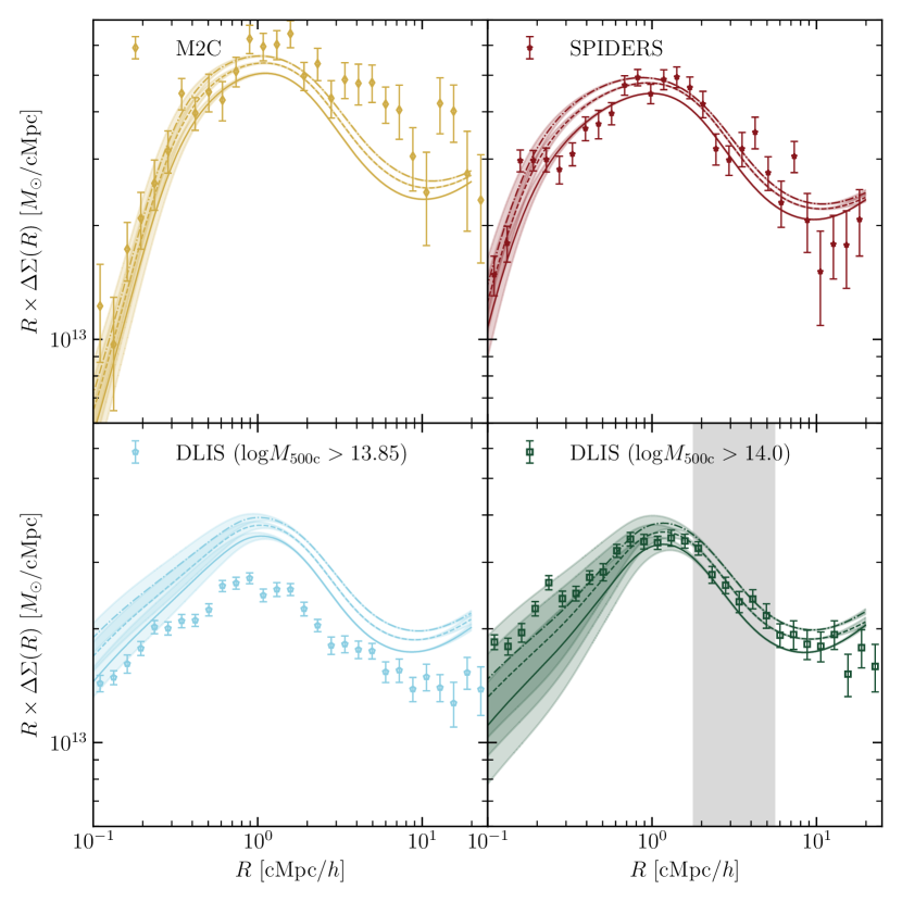
Figure 2: Data points with error bars show mean excess mass density profiles $\Delta\Sigma(R)$ (in comoving units) for three publicly available lens catalogues, calculated with the code dsigma from a UNIONS shape catalogue. The DESI Legacy Imaging Survey (DLIS) catalogue is used with two choices for the minimum mass in the subsample (bottom panels). The value $\Omega_{\rm m}=0.3$ is used to convert angles and redshifts to distances. Also overlaid are the corresponding mean profiles from simulations with $\Omega_{\rm m}=0.3$ and $\sigma_{8}=0.7,0.8,0.9$ (solid, dashed, dash-dot respectively). For DLIS, the match is performed using all simulated halos above the quoted mass limit. For M2C and SPIDERS, when taking the mean we weight the contribution of each simulated halo by the relative number of halos at that mass in the observed sample. We have corrected the simulated profiles for mis-centering, based on fits to the observed data. The grey band in the bottom right panel indicates the radial range used to compare the observed profile to the simulated profiles in our cosmological analysis.

The observable in cluster lensing is the excess surface mass density, $\Delta\Sigma$. It can be expressed as the difference between the average surface mass density within a projected radius $R$, and the mass density at that radius:

$$\Delta\Sigma(r)=\overline{\Sigma}(R)-\Sigma(R)\,,$$ (1)

where

$$\overline{\Sigma}(R)=\frac{2}{R^{2}}\int_{0}^{R}R^{\prime}\Sigma(R^{\prime})\,dR^{\prime}\,,$$ (2)

and the surface mass density is a 2D projection of the 3D density profile $\rho(r)$:

$$\Sigma(R)=2\int_{R}^{\infty}\frac{\rho(r)r}{\sqrt{r^{2}-R^{2}}}\,dr\,.$$ (3)

The $\Delta\Sigma$ profile of a foreground lens is simply related to the tangential shear $\gamma_{\rm t}$ of background sources through

$$\Delta\Sigma(R)=\gamma_{\rm t}(R)\Sigma_{\rm crit}\,,$$ (4)

where $\Sigma_{\rm crit}$ is the critical density defined below, that depends on the source and lens redshifts. In practice we measure the tangential shape, $e_{\rm t}$, of many background sources around a large number of lenses, and stack the measurements, with appropriate weights, into a composite $\Delta\Sigma$ profile. The composite profile is calculated by summing over lens-source pairs (l–s) in radial bins,

$$\Delta\Sigma(R)={\rm boost}(R)\times\frac{\sum_{\rm l-s}w_{\rm sys,l}w_{\rm s}e_{\rm t}\langle\Sigma_{\rm crit,l}^{-1}\rangle}{\sum_{\rm l-s}w_{\rm sys,l}w_{\rm s}\langle\Sigma_{\rm crit,l}^{-1}\rangle^{2}}\,,$$ (5)

where $w_{\rm s}$ is the source weighting related to the shape noise, $w_{\rm sys,l}$ is a lens weighting chosen to reduce the impact of lens selection biases, and

$$\Sigma_{\rm crit,l-s} =\frac{c^{2}}{4\pi G}\frac{\chi_{\rm s}}{\chi_{\rm l}(\chi_{\rm s}-\chi_{\rm l})(1+z_{\rm l})}\,,$$ (6)

$$\langle\Sigma_{\rm crit,l}^{-1}\rangle =\int\Sigma_{\rm crit,l-s}^{-1}n(z_{\rm s})\,dz_{\rm s}\,.$$ (7)

The $\chi$ indicate comoving distances. For the public lens catalogues adopted, we set $w_{\rm sys,l}=1$ for all sources. Instead of using the inverse $\Sigma_{\rm crit}$ value for each lens-source pair, we calculate the average defined above, as the version of the ShapePipe catalogue used in this work does not have photo-zs associated with individual sources. The mean inverse $\Sigma_{\rm crit}$ in Eq. (7) is calculated using the distribution of galaxies in a matched redshift distribution $n(z)$, detailed in Section 2.1.

The boost term comes from contamination of the source galaxy sample by cluster members that do not contribute to the lensing signal. This reduces the mean value of the shear, and needs to be corrected for when estimating $\Delta\Sigma$. The boost factor in a radial bin can be estimated by comparing lens-source pairs to random-source pairs,

$${\rm boost}(R)=\frac{\sum_{\rm l-s}w_{\rm sys,l}w_{\rm l-s}}{\sum_{\rm r-s}w_{\rm sys,l}w_{\rm l-s}}\,.$$ (8)

We compute mean $\Delta\Sigma$ profiles for the three public galaxy cluster catalogues; M2C, SPIDERS and DLIS, using UNIONS galaxy shapes and the dsigma package (Lange & Huang, 2022). In Appendix A we show the size of the boost factor correction for each cluster sample used in this work.

It is important to note that we are assuming $\langle e_{\rm t}\rangle=\gamma_{t}$, i.e. that the average ellipticity of a large number of galaxies is equal to the tangential shear. The true observable is in fact the reduced shear,

$$g_{\rm t}=\frac{\gamma_{\rm t}}{1-\kappa}\,.$$ (9)

The convergence $\kappa$, proportional to the surface mass density, is small at large projected radii, but increases towards the centre of a cluster. The error incurred in assuming $g_{\rm t}=\gamma_{\rm t}$ (i.e. $\kappa\ll 1$) will be less than $1\%$ in the infall region, and thus will not impact our cosmological constraints. But assuming $g_{\rm t}=\gamma_{\rm t}$ leads to an overestimate of $\Delta\Sigma$ in the inner region, which will affect fits to the inner profile. In Appendix B we show that $\kappa$ falls below $20\%$ in the radial range adopted for our fits, justifying the reduced shear approximation.

In addition to the boost correction based on random-source pairs, Singh et al. (2017) have shown that subtracting a $\Delta\Sigma$ profile calculated from random-source pairs (without any boost correction) leads to a cleaner profile and smaller uncertainties. To apply this correction, we generate a set of random locations $20\times$ larger than the lens sample size, drawn uniformly from the UNIONS footprint, and assign random redshifts picked from the same redshift distribution as the lenses. We calculate the resulting $\Delta\Sigma$ profile from Eq. (5), and subtract it from our observed profile. To calculate the uncertainty, a jackknife resampling method is used. The region is split into $N_{\rm jk}=100$ sub-regions of roughly equal size, then the covariance between radial bins $i$ and $j$ is given by

$${\rm Cov}_{ij}=\frac{N_{\rm jk}-1}{N_{\rm jk}}\sum_{k=1}^{N_{\rm jk}}\left(\Delta\Sigma_{k}(R_{i})-\Delta\Sigma(R)\right)\left(\Delta\Sigma_{k}(R_{j})-\Delta\Sigma(R)\right)\,.$$ (10)

We also tested the impact of a lens magnification bias, when lenses are themselves magnified by foreground structure which can contribute to the shear signal. This is more impactful for galaxy-galaxy lensing. Even when assuming extreme responses of lenses to magnification, values, up to $\alpha_{\rm lens}=10$ (Unruh et al., 2020), the impact on the recovered $\Delta\Sigma$ is $\lesssim 1\%$, such that we can safely neglect this effect.

We calculate $\Delta\Sigma(R)$ using $30$ logarithmically spaced radial bins from $0.1-25\,$cMpc$/h$. Fig. 2 shows the resulting profiles for each of the cluster samples. We note that the conversion from angles and redshifts to distances is affected by the choice of $\Omega_{\rm m}$. In Fig. 2 we have set $\Omega_{\rm m}=0.3$. We investigate how this choice of fiducial value impacts the recovered $r_{\rm sp}$ in Appendix C. We test the correlation between radial bins by calculating the mean off-diagonal correlation in the correlation matrix (removing the on-diagonal unity terms, and finding the average). This gives $\sim\!0.1$ for all cluster samples, indicating little correlation between bins.

4.2 Comparison to simulations

The mean density profile from simulated halos, and a corresponding $\Delta\Sigma$ profile is calculated. First the 2D surface mass density as a function of projected cluster-centric distance $\Sigma(R)$, shown in Eq. (3), is found from the density extracted from particle data. Then a corresponding $\Delta\Sigma$ profile is found using Eq. (1). When computing a final $\Delta\Sigma$ profile from observations, values for $H_{0}$ and $\Omega_{\rm m}$ are needed to convert angles and redshifts into radii and distances. The value of $H_{0}=70\,$km s${}^{-1}\,$Mpc^-1 used in the simulations is kept fixed throughout. As we are comparing to simulations with five different possible values for $\Omega_{\rm m}$, five $\Delta\Sigma$ profiles are calculated for each cluster sample. Then when comparing observations to simulations, profiles with $\Omega_{\rm m}=0.3$, for example, will be compared to the simulations with $\Omega_{\rm m}=0.3$ and $\sigma_{8}=0.7,0.75,0.8,0.85,0.9$ to find the best fit.

To obtain accurate cosmological constraints, we need to consider carefully the sample selection for both the observed clusters and the simulated halos. Ideally, the observed cluster samples would be pure (containing only systems over some mass) and complete (containing all systems over that mass); then we would compare these to a mass-limited sample of simulated halos. Uncertainties in cluster masses complicate the situation, however, scattering clusters above the mass cut out of the sample and clusters under the mass cut into the sample — an Eddington bias. Given the steep slope of the mass function, the dominant effect of errors in mass is to add low-mass systems to the sample.

Another complicating effect is that of mis-centering. Although mis-centering causes a shift smaller than our measurement uncertainties in the infall region, we still include the effect for visual comparison between simulated and observed halos in the inner region, and for accurate profile fitting. There may also be systematic offsets in the masses recovered from the lensing profiles and the catalogue masses determined from observational proxies such as X-ray luminosity. We will consider these effects in future work.

For each of the cluster samples, we generate a matched profile from the simulations, also including the effects of mass scatter and mis-centering. To make the corresponding simulation profile for the DLIS sample, we use the concentration values for each simulated halo identified by AHF to convert their masses from $M_{200{\rm c}}$ to $M_{500{\rm c}}$, in line with the mass definition used in the DLIS catalogue. When iterating over each halo in the simulation, first an individual mass-scatter is added by drawing from a Gaussian distribution with a width equal to the quoted mass uncertainty in the corresponding observed catalogue. A density profile is found by taking the mean profile of the mass-scattered halos. Then, drawing random values for the fraction of sources with an offset and the amplitude of the offset distribution based on their mean and uncertainty from the corresponding best-fits (see Section 4.3), we create a mis-centered $\Delta\Sigma$ profile. This is repeated $100$ times, and the average of this profile and the $1\sigma$ spread of all the profiles is used as the corresponding simulated profile and its uncertainty. The resulting uncertainties are larger than those coming from a bootstrap process when creating the density profile from the collection of halos, and so we use these uncertainties when comparing between simulated and observed profiles.

To compare observed and simulated samples, we need to account for completeness in the former. Considering Fig. 1, only the DLIS catalogue is reasonably complete. To create matched simulation profiles for SPIDERS and M2C shown in Fig. 2, we weight the contribution of each simulated halo by the ratio of the observed and simulated mass functions. The incompleteness of these catalogues nonetheless suggests they may be prone to selection biases related to dynamical state, so we do not use these samples to derive cosmological constraints.

The lines in Fig. 2 show the $\Delta\Sigma$ profiles of the matched halo samples in the suite of simulations, corresponding to the observed cluster samples used in this work and outlined in Table 1. Each line is from a simulation with $\Omega_{\rm m}=0.3$, and $\sigma_{8}=0.7,0.8,0.9$ given by the solid, dashed, and dashed dot lines. M2C exhibits excess signal in the infall region, at distances of $2-3\,$cMpc/$h$ (top left panel). This may indicate the catalogue is biased towards dynamically relaxed systems with a larger peak of X-ray emission, which have more extended infall regions (Haggar et al., 2020). For the DLIS sample with log$M_{500{\rm c}}<13.85$ (bottom left panel), the signal is considerably weaker than predicted in the simulations. This is likely due to the inclusion of spurious systems caused by projection effects and large redshift uncertainties of photometrically identified cluster members. We also show a DLIS profile with a higher mass threshold, ‘DLIS high’, along with predictions for simulated samples with the same mass range (bottom right panel). This leads to a much better agreement between the observed and simulated profiles.

4.3 Fitting procedure

Parameter	Fiducial value	Prior	Description
log$\,\rho_{s}\,/\,[h^{2}M_{\odot}/{\rm cMpc}^{3}]$	log$(10^{3}\,\rho_{\rm m})$	log$([10^{1},10^{7}]\,\rho_{\rm m})$	Density at scale radius	}3*[Einasto]
log$\,r_{s}\,/\,[$cMpc$/h]$	log$(0.07\,r_{200{\rm m}})$	log$([0.01,0.45]\,r_{200{\rm m}})$	Scale radius
log$\,\alpha$	-1	log$([0.03,0.4])$	Slope of inner Einasto profile
log$\,r_{t}\,/\,[$cMpc$/h]$	log$(r_{200{\rm m}})$	log$([0.455,3]\,r_{200{\rm m}})$	Truncation radius for inner Einasto profile	}2*[Truncation]
log$\,\beta$	0	$[-1,1.3]$	Sharpness of truncation
log$\,\delta_{1}$	1	$[0,2]$	Overdensity at the pivot radius	}3*[Infalling]
log$\,\delta_{\rm max}$	2	$[0,3+{\rm log}(2)]$	Overdensity in the halo centre
log$\,s$	-1	$[-2,2{\rm log}(2)]$	Slope of the infalling term
log$\,\sigma_{\rm off}\,/\,[$cMpc$/h]$	-0.5	$[-2,0]$	Amplitude of offset distribution	}2*[Mis-centering]
$f_{\rm off}$	0.3	$[0,1]$	Fraction of lenses with offset

Table 2: Parameters used to fit a $\Delta\Sigma$ profile. The reference value of $\rho_{\rm m}$ and $r_{200{\rm m}}$ are calculated at $z=0$ as we adopt comoving units, and using the same $\Omega_{\rm m}$ value as used when calculating the $\Delta\Sigma$ profile from the observed shear profile.

We fit the mean observed excess mass profiles using the 3D density profile model of Diemer (2022), as this includes an infalling term not present in the Navarro-Frenk-White (NFW) (Navarro et al., 1996) or Einasto profiles (Einasto, 1965). This model is designed to be a good fit, with $\lesssim 5\%$ accuracy, to mean dark matter density profiles over a wide range of mass, redshift and cosmology. The model represents an improvement over an earlier version (Diemer & Kravtsov, 2014), which has been used in the literature to estimate the splashback radius of stacked clusters. The new model has been shown to outperform the earlier model and be more physically motivated (Diemer, 2022). It is given by

$$\rho(r) =\rho_{\rm orbit}(r)+\rho_{\rm infall}(r)\,,$$ (11)

$$\rho_{\rm orbit}(r) =\rho_{s}\,\exp{\left(-\frac{2}{\alpha}\left[\left(\frac{r}{r_{s}}\right)^{\alpha}-1\right]-\frac{1}{\beta}\left[\left(\frac{r}{r_{t}}\right)^{\beta}-\left(\frac{r_{s}}{r_{t}}\right)^{\beta}\right]\right)}\,,$$

$$\rho_{\rm infall}(r) =\rho_{\rm m}\,\left(1+\delta_{1}/\sqrt{\left(\delta_{1}/\delta_{\rm max}\right)^{2}+\left(r/r_{\rm pivot}\right)^{2s}}\right)\,,$$ (12)

where

$$r_{\rm pivot}(z)=\left(\frac{3M_{200{\rm m}}}{4\pi\times 200\,\rho_{\rm m}(z)}\right)^{1/3}\,.$$ (13)

When fitting simulated density profiles, the parameter $\rho_{\rm m}$ is left free to minimize the residuals. When fitting observed $\Delta\Sigma$ profiles, $\rho_{\rm m}$ is fixed to the matter density using the same assumed value of $\Omega_{\rm m}$ which converts angles and redshifts to distances. The values for $M_{200{\rm m}}$ listed in Table 1 are used to calculate the pivot radius, but the fits are fairly insensitive to this choice.

The procedure outlined in Diemer (2022) Appendix A is used to fit both the observed $\Delta\Sigma$ profiles, and the simulated density profiles. When fitting $\Delta\Sigma$, we start by generating a density profile using the model of Eq. (12) and a set of model parameters, and then calculate the associated $\Delta\Sigma$ profile. As pointed out in Diemer (2024), values for $\alpha$ and $\delta_{\rm max}$ can be fixed when fitting mean density profiles over the whole radial range, leading to narrower and unbiased posteriors for the remaining parameters. We first perform the full least-squares regression procedure, varying all parameters. We then use the Preconditioned Monte Carlo (PMC) algorithm, pocoMC (Karamanis et al., 2022b, a), to sample from the correlated, non-Gaussian parameter space and obtain uncertainties on the fitting parameters. The initial state of the PMC is the best-fit model from the least-squares regression, and the prior comes from combining the Gaussian uncertainty from the least-squares fit with the uniform prior in Table 2. Finally we repeat this procedure, fixing log$\alpha$ and log$\delta_{\rm max}$ to their median values from the initial MC chain. We include a mis-centering term into the fitting procedure following e.g. Johnston et al. (2007). It modifies the profile by constructing it as the sum of a term with no offset, and a term where the centre is mis-identified:

$$\Sigma(R)=(1-f_{\rm off})\Sigma_{0}(R)+f_{\rm off}\Sigma_{\rm off}(R)\,.$$ (14)

where $f_{\rm off}$ is the unknown fraction of sources with an offset. $\Sigma_{0}$ is the term in Eq. (3). The offset surface density is given by

$$\Sigma_{\rm off}(R|R_{\rm off}) =\frac{1}{2\pi}\int_{0}^{2\pi}\Sigma_{0}\left(\sqrt{R^{2}+R_{\rm off}^{2}+2RR_{\rm off}\cos(\theta)}\right)\,d\theta\,,$$ (15)

$$\Sigma_{\rm off}(R) =\int_{0}^{\infty}p(R_{\rm off})\Sigma_{\rm off}(R|R_{\rm off})\,dR_{\rm off}\,.$$ (16)

The offset probability follows a Rayleigh distribution,

$$p(R_{\rm off})=\frac{R_{\rm off}}{\sigma_{\rm off}^{2}}\exp\left(-\frac{R_{\rm off}^{2}}{2\sigma_{\rm off}^{2}}\right)\,.$$ (17)

The amplitude of the offset distribution, $\sigma_{\rm off}$, has units of cMpc$/h$. Then there are two more free parameters in the fitting, $f_{\rm off}$ and $\sigma_{\rm off}$. Table 2 summarizes the fit parameters and their priors, and gives a brief description of each.

We calculate the average, upper and lower bounds for $r_{\rm sp}$ and $\Delta\Sigma$ by recomputing their values for each parameter set in the final MC chain, and finding the median and $68\%$ confidence interval.

5 Results

Our analysis proceeds through three main steps:

1. In Section 5.1 we compare the amplitude of the $\Delta\Sigma$ profile found from the DLIS high cluster sample to the expected sample in a suite of cosmological simulations. This constrains $\Omega_{\rm m}$ and $\sigma_{8}$.

2. In Section 5.2 we then fit a 3D density profile model to the observed $\Delta\Sigma$ profile for each cluster sample, deriving estimates of the splashback radii.

3. In Section 5.3 we explore how two features of the infall region, the splashback radius and the truncation radius in Eq. (12), could be used to constrain cosmology.

5.1 Cosmological constraints from profile comparisons

Of our four cluster samples, DLIS high is the closest to being complete, as argued by Wen & Han (2024). Thus, we will compare the mean projected mass profile for this sample to the simulated profiles in order to constrain cosmological parameters. We use the DLIS high sample with $M_{500{\rm c}}>10^{14}M_{\odot}/h$ as this produces a signal comparable to that expected in simulations, as seen in Fig. 2, whereas at lower masses the DLIS sample may be contaminated by projected systems with overestimated masses. Of course we can not be sure we have removed all interlopers from the sample, and there may still be a bias in the observed $\Delta\Sigma$ profile. In creating the matched simulation profiles, we convert the simulated halo masses from $M_{200{\rm c}}$ to $M_{500{\rm c}}$ by adopting the cosmological parameters of the particular simulation, and using the NFW concentration parameter determined by AHF. The converted masses have been mass-scattered, such that we are including the effect of low-mass systems entering the sample, and high mass systems leaving the sample. We then take the mean profile of all simulated halos with $M_{500{\rm c}}>10^{14}M_{\odot}/h$. Though the redshift distribution differs between the simulated and observed clusters, the infall region does not vary significantly with redshift when using comoving units of distance as explored in Mpetha et al. (2024).

We use the results in Eq. (14) of Mpetha et al. (2024) to define the radial range of the infall region over which to compare the simulated and observed profiles. Adopting the constants associated with UNIONS gives an angular radius at which we expect the signal in the infall region to peak of $\theta_{\rm peak}=0.254\,$deg. Considering Fig. 4 of Mpetha et al. (2024), we use an angular range of log$(\theta_{\rm peak})\pm 0.25\,$dex. To convert the angular range to a radial range, we use the mean redshift of the DLIS high sample and adopt a fiducial value of $\Omega_{\rm m}=0.3$. This translates into a radial range of $1.77-5.61\,$cMpc$/h$. This range is shown as the grey band in Fig. 2.

In each cosmological simulation with a given value of $\Omega_{\rm m}$ and $\sigma_{8}$, the amplitude of the simulated profile in the defined radial range is compared to the amplitude of the observed profile in the same range. We always compare observed and simulated profiles generated with the same value of $\Omega_{\rm m}$. Each simulation in Fig. 3, represented by a black dot, has an associated $\chi^{2}$ of the difference between the simulated and observed profiles in the infall region. The best fitting simulation is $\Omega_{\rm m}=0.3$, $\sigma_{8}=0.8$. We fit a 3D paraboloid to the $\chi^{2}$ values, and plot the minimum of the paraboloid with a green cross; this point has a reduced $\chi^{2}$ of $\chi_{r}^{2}=0.98$. Finding the contour with $\Delta\chi^{2}=1$ above the minimum gives marginalised $68.3\%$ constraints of $\Omega_{\rm m}=0.29\pm 0.05$ and $\sigma_{8}=0.80\pm 0.04$. To draw the 2D $68.3\%$ and $95.5\%$ confidence regions we plot contours of $\Delta\chi^{2}=2.3$ and $\Delta\chi^{2}=6.81$ from the minimum. Also plotted are GetDist (Lewis, 2019) chains from Planck (Planck Collaboration et al., 2020) and eROSITA (Ghirardini et al., 2024). It should be noted that paraboloid fit to the $\chi^{2}$ surface is itself uncertain. Drawing from the correlated best-fit parameters for the 3D paraboloid produces a set of possible paraboloids, leading to a variation in the reported constraints of $\pm 0.01$.

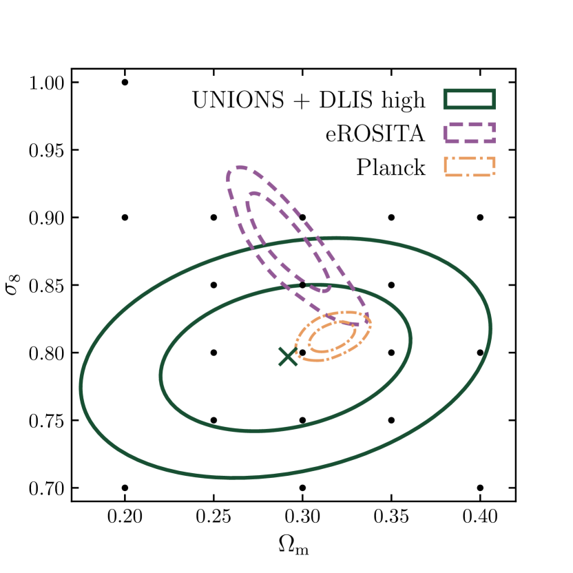
Figure 3: Cosmological constraints from comparing simulated dark matter halos, with UNIONS weak lensing profiles of DESI Legacy Imaging Survey (DLIS) galaxy clusters with $M_{500{\rm c}}>10^{14}M_{\odot}/h$. The observed profile in the infall region is compared to the profile in each of a suite of $19$ cosmological simulations varying $\Omega$ and $\sigma_{8}$ (black points) and a goodness-of-fit $\chi^{2}$ value is calculated for each. A 3D paraboloid is fit to these $\chi^{2}$ values. The best fit cosmology is indicated with a green cross, $68.3\%$ and $95.5\%$ confidence regions at $\Delta\chi^{2}=2.3,6.81$ from the minimum are overlaid.

5.2 Fits to observed weak lensing profiles

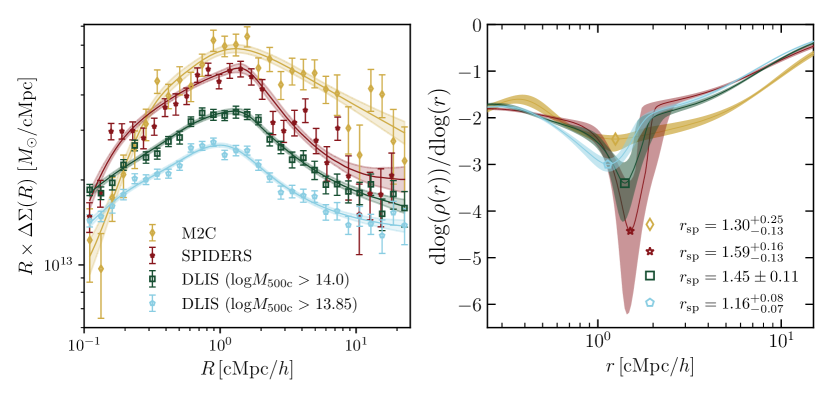
Figure 4: Left: Observed excess surface mass densities for each of the cluster samples. For DLIS, we show the result from two different choices for the lower mass limit. These profiles are fitted with a 3D density profile model (Diemer, 2022). Right: The gradient of the 3D density profile fit is used to identify the splashback radius of each cluster sample.

The left panel of Fig. 4 shows fits to mean mass profiles determined from weak lensing (in comoving units) in the four cluster samples. The fits differ from the simulation profiles shown in Fig. 2 at large $R$ due to projection effects—the simulation profiles are found using the 3D density profile in spherical shells. The fits all have a reduced $\chi^{2}$ of 1.03. The M2C sample has the largest amplitude, as it has the largest mean mass. It also has a slightly lower mean redshift than the SPIDERS sample. The DLIS sample has both the lowest mean mass and the highest mean redshift. Selection effects in the M2C meta-catalogue, leading to a larger fraction of dynamically relaxed clusters, may explain the excess signal at large radii. Resulting fit parameters are shown in Table 3, and the $68.3\%$ and $95.5\%$ error contours derived from the corresponding PMC chain are shown in Fig 5. The right panel of Fig. 4 shows the logarithmic density profile from the fitting procedure with the splashback radius indicated. We make the simplifying assumption that the splashback radius is the point where the gradient of the density profile is steepest, though it has been shown these two features are not always equivalent (Diemer, 2020).

From the best-fit density profile, we can derive $r_{200{\rm c}}$ and $M_{200{\rm c}}$ by locating the radius at which the average density within the halo,

$$\langle\rho(<r^{\prime})\rangle=\frac{3\int_{0}^{r^{\prime}}r^{2}\rho(r)dr}{r^{\prime 3}}\,,$$ (18)

reaches $200\rho_{\rm c}$. Because our cluster samples are mass-limited and each cluster mass is uncertain to $\sim\!0.2\,$dex, lower-mass systems are scattered into the sample, and clusters with masses in the mass-cut will be scattered out of the sample. This causes a biased sample, with a true mean mass smaller than observed. We include this effect in the simulation profiles in Fig. 2, finding it leads to an observed mean mass $\sim\!25\%$ larger than the true mean mass of the sample. When comparing our lensing-based masses in Table 3 to the reported masses in Table 1, we find the reported masses are $28\%$, $41\%$ and $39\%$ larger than the lensing masses for M2C, DLIS high and SPIDERS respectively. Therefore, the mass-scattering effect is a large cause for our discrepant masses, but not the only cause. Other selection effects could be biasing the reported masses in Table 1.

There are other reasons to be cautious about the masses reported from our fitting procedure in Table 3. There is a large degeneracy between parameters of the inner profile and mis-centering parameters. When $\alpha$ is fixed, although this does not significantly affect our inference of properties of the infall region, it may have a strong impact on the best-fit $f_{\rm off}$ and $\sigma_{\rm off}$, which in turn affects the amplitude of the 3D density profile in the inner region, and the resulting mass estimates. Another reason for the discrepancy in mass estimates could be the effect of baryonic processes on the density profile. In Fig. 1 of Castro et al. (2021), for example, the authors find a $\sim\!10\%$ difference in $M_{200{\rm c}}$ when comparing hydrodynamical and dark-matter only simulations. For these reasons, we will derive cosmological constraints assuming the masses reported in Table 1 are correct, correcting only for Eddington bias (which is included in the simulations when creating matched simulation profiles and performing the profile comparison in Section 5.1). We could instead create matched simulation profiles assuming our slightly lower lensing-derived masses are correct. Doing this shifts the contour in Fig. 3 towards the upper-left corner, and leads to constraints of $\Omega_{\rm m}=0.19\pm 0.07$, $\sigma_{8}=0.86\pm 0.04$. These results are consistent within $1\sigma$, but suggest uncertainties in cluster masses could increase our systematic errors by $\sim\!~50\%$, if not addressed in future follow-up.

Fig. 5 shows how well parameters of the infall region, notably the truncation radius $r_{t}$, can be determined. The observed M2C $\Delta\Sigma$ profile has the largest uncertainties due to the smallest number of clusters, and thus the fit parameters have the largest uncertainties in this case. Parameters of the infall region in particular are not well-constrained, and the splashback radius is smaller than expected. This could be related to the significant mis-centering in these clusters.

By comparison, the DLIS high sample has the smallest fraction of sources with a centering offset, $22\%$, with a small mis-centering amplitude, $54\,$kpc$/h$. The small fraction, with a relatively small offset indicates the BCG centroids in the DLIS catalogue are performing well. M2C and SPIDERS both have a large fraction of mis-centered sources, with $f_{\rm off}=85\%$ and $79\%$ respectively, where M2C has a larger offset amplitude offset ($120\,$kpc$/h$ compared to $54\,$kpc$/h$). As M2C is constructed from purely X-ray and SZ selected clusters, which contain larger centering uncertainties, it is no surprise it has the largest fraction of mis-centered clusters.

A comparison between the case where log$\,\alpha$ and log$\,\delta_{\rm max}$ are fixed and left free in the fitting procedure is shown in Appendix D.

	M2C	DLIS high	SPIDERS
${\rm log}\,\rho_{s}$	$15.51^{+0.43}_{-0.44}$	$14.49^{+0.19}_{-0.2}$	$14.05\pm 0.16$
${\rm log}\,r_{s}$	$-1.15^{+0.2}_{-0.19}$	$-0.78\pm 0.1$	$-0.46\pm 0.08$
${\rm log}\,\alpha$ (fixed)	$-0.88$	$-1.00$	$-1.04$
${\rm log}\,r_{t}$	$0.21^{+0.22}_{-0.29}$	$0.03\pm 0.03$	$0.05\pm 0.03$
${\rm log}\,\beta$	$0.47^{+0.55}_{-0.58}$	$0.78^{+0.22}_{-0.23}$	$0.79^{+0.23}_{-0.24}$
${\rm log}\,\delta_{1}$	$1.64\pm 0.03$	$1.39\pm 0.03$	$1.96\pm 0.03$
${\rm log}\,\delta_{\rm max}$ (fixed)	$2.94$	$2.69$	$2.44$
${\rm log}\,s$	$0.35\pm 0.02$	$0.31\pm 0.01$	$0.26\pm 0.02$
$f_{\rm off}$	$0.85\pm 0.05$	$0.22\pm 0.11$	$0.79\pm 0.16$
${\rm log}\,\sigma_{\rm off}$	$-0.92\pm 0.06$	$-1.24^{+0.24}_{-0.22}$	$-1.27\pm 0.06$
$r_{\rm sp}\,/\,[$cMpc$/h]$	$1.30^{+0.25}_{-0.13}$	$1.45\pm 0.11$	$1.59^{+0.16}_{-0.13}$
$r_{200{\rm c}}\,/\,[$cMpc$/h]$	$1.01\pm 0.04$	$0.82^{+0.03}_{-0.05}$	$0.93^{+0.04}_{-0.05}$
$M_{200{\rm c}}\,/\,[M_{\odot}/h]$	$14.37\pm 0.05$	$14.10^{+0.05}_{-0.08}$	$14.27^{+0.05}_{-0.07}$

Table 3: Parameter values from the profile fits for each of the three cluster samples. Profiles, in comoving units, were created using $\Omega_{\rm m}=0.3$ to convert angles and redshifts to distances. DLIS high uses a mass limit of $M_{500{\rm c}}>10^{14}M_{\odot}/h$. We also include derived results for the splashback radius $r_{\rm sp}$ found as the radius of the steepest slope of the logarithmic density profile. In all cases the $68.3\%$ credible region is quoted.

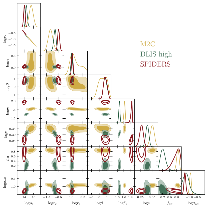
Figure 5: $68.3\%$ and $95.5\%$ credible regions for parameters of the 3D density profile model of Diemer (2022), fitted to the observed $\Delta\Sigma$ profile of three publicly available cluster catalogues. Chains are created using a Preconditioned Monte Carlo algorithm (Karamanis et al., 2022a, b)

5.3 Cosmological constraints using characteristic radii

In Section 5.1, we derived for the first time cosmological constraints based on the amplitude of the shear signal in the infall region. As explored in (Haggar et al., 2024; Mpetha et al., 2024), specific features of the infall region provide another possible test of cosmology. Extracting specific features, as opposed to comparing the profile over the entire infall region, may introduce model dependence and reduce the constraining power, but should produce results less dependent on vertical shifts of the shear profile. Here we explore two features, the splashback radius, and a specific feature of the density profile model in Eq. (12), the truncation radius $r_{t}$. In both cases we find that the number of clusters in our three samples are not sufficient to obtain useful cosmological constraints.

5.3.1 Splashback radius

Fig. 6 shows previously-measured splashback radii from the literature, as a function of the mean mass $M_{200{\rm c}}$ of the cluster sample. We also include our own values from DLIS, SPIDERS, and M2C, measured from the UNIONS weak lensing profiles. The grey lines are the simulation results, with darker colours indicating higher values of $S_{8}$. The uncertainty in the simulation results, indicated by a shaded band, is generally small except at large masses where sample variance is significant. It can be seen that several literature values, including our own, are low compared to expectations from simulations. However this is an unfair comparison, due to the mass-scatter effect described in Section 4.2. We expect there to be more low-mass systems in the observed catalogue, meaning we expect $r_{\rm sp}$ to be smaller. The arrows on values from this work show the mean mass when a $25\%$ Eddington bias, found in our simulation profiles, is removed. When comparing the inferred values to the splashback radii in the matched simulation profile in Fig. 2 for the best fit cosmology of our analysis in Section 5.1, $\Omega_{\rm m}=0.3$ and $\sigma_{8}=0.8$, the reported splashback is smaller than the expected value in each case, by $0.71\sigma$, $0.36\sigma$ and $1.8\sigma$ for DLIS high, SPIDERS and M2C respectively. It can be seen that the observed M2C profile differs significantly from expectations in Fig. 2, likely due to selection effects in the catalogue, so it is no surprise the recovered $r_{\rm sp}$ is discrepant.

The splashback radii in Fig. 6 have been calculated assuming different values of $\Omega_{\rm m}$, and the underlying cluster catalogues may also be subject to selection effects. Given these uncertainties, we do not attempt joint cosmological constraints on $\Omega_{\rm m}$ and $\sigma_{8}$ using the splashback radius, but note that this will be possible with future data (Mpetha et al., 2024).

In Eq. (4) of Haggar et al. (2024), the authors present a relationship between the splashback radius, $\Omega_{\rm m}$ and $\sigma_{8}$,

$$r_{\rm sp}=a^{\prime}+b^{\prime}\left(\frac{\sigma_{8}}{\Omega_{\rm m}^{0.3}}\right)\,,$$ (19)

calibrated using the same cosmological simulation suite as used in this work, but considering halos at $z=0$ only. We repeat their method using the matched simulation profiles in Fig. 2, leading to values of $a^{\prime}=0.82\pm 0.09$, $b^{\prime}=0.57\pm 0.08$ for DLIS high; $a^{\prime}=0.95\pm 0.12$, $b^{\prime}=0.64\pm 0.10$ for SPIDERS; and $a^{\prime}=0.92\pm 0.09$, $b^{\prime}=0.75\pm 0.08$ for M2C. Using the value $\Omega_{\rm m}=0.3$ assumed in computing splashback radii, the associated $\sigma_{8}$ can be predicted. This gives $\sigma_{8}=0.76\pm 0.20$, $\sigma_{8}=0.70^{+0.25}_{-0.22}$, and $\sigma_{8}=0.36^{+0.25}_{-0.15}$ for DLIS high, SPIDERS and M2C respectively. While not yet competitive with other tests in the literature, DLIS high and SPIDERS are consistent with the results of Section 5.1. Considering the difference between the observed and simulated profiles for the M2C catalogue in Fig. 2, it is not surprising the constraint on $\sigma_{8}$ is also discrepant.

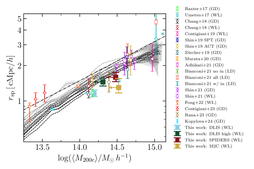
Figure 6: Dashed lines show the splashback radius $r_{\rm sp}$ as a function of mass in the $19$ cosmological simulations used in this work. Darker line colour corresponds to higher $S_{8}$ for that simulation, ranging from $0.57$ when $(\Omega_{\rm m},\sigma_{8})=(0.2,0.7)$, to $1.04$ with $(0.4,0.9)$. Uncertainties are given by shaded bands. The black dash-dot line is $2r_{200{\rm c}}$. Also overlaid are splashback radii from the literature, where mean masses of the cluster samples have been converted into $M_{200{\rm c}}$, and splashback radii into comoving units. These splashback radii have been measured from cluster profiles created using different methods: galaxy number density profiles (GD), weak lensing profiles (WL), and luminosity density profiles (LD). The four $r_{\rm sp}$ values from this work are included. In Bianconi et al. (2021), the authors use three versions of their catalogue to derive a splashback radius: including all clusters (‘all’), only including clusters which contain infalling groups (‘w/ in’), and only including clusters without any infalling groups (‘no in’). The arrows on the values from this work give an approximate indication of the true masses of our cluster samples, with the Eddington bias removed.

5.3.2 Truncation radius

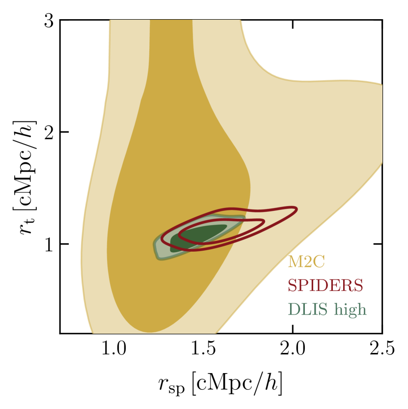
Figure 7: The best-fit splashback radius and truncation radius found from fits to UNIONS weak lensing profiles of three galaxy cluster catalogues.

As pointed out in Diemer (2024), the truncation parameter $r_{\rm t}$ of the density profile model in Eq. (12) could provide a more robust tracer of the accretion history of clusters than the steepest slope of the density profile. The relationship between the point of steepest slope, $r_{\rm steep}$, and the splashback radius is not straightforward. Furthermore, the inferred value of $r_{\rm steep}$ is very sensitive to the fitting function/algorithm used (Diemer, 2020), whereas $r_{t}$ is shown to be a more stable indicator of accretion rate (Diemer, 2024). Fig. 7 shows the relationship between the inferred splashback radius and the truncation radius. For SPIDERS, uncertainty in the truncation radius is smaller than uncertainty in the splashback radius by a factor of two, and for DLIS high it is smaller by $\sim\!0.2\,$cMpc$/h$.

The value of $r_{\rm t}$ in Table 3 can be compared to the values from the matched simulation profiles in Fig. 2, over the whole grid of $\Omega_{\rm m}$ and $\sigma_{8}$. Doing so provides cosmological constraints consistent with those in Section 5.1, but with larger errors and greater dependence on systematics, particularly in the profile fitting, so we do not report these results.

6 Discussion

The mean formation time of dark matter halos depends on the values of cosmological parameters. Measuring the mass distribution in the infall region of galaxy clusters provides a novel method to estimate their average formation time. In cosmologies with low values of $\Omega_{\rm m}$ and high values of $\sigma_{8}$, clusters form earlier. This means they have more time to accrete material and become dynamically relaxed, leading to a more extended profile, and more mass in the infall region. In this work, we have used weak lensing profiles of cluster samples drawn from three publicly available catalogues to measure the mass distribution in the infall region, thereby constraining the background cosmology in which these clusters formed. The dependence of cluster formation time on cosmology is nearly orthogonal to the dependence of the halo mass function on cosmology. Thus, combining these two observables in a galaxy cluster catalogue can break the degeneracy in $\Omega_{\rm m}$ and $\sigma_{8}$ without requiring external data sets.

We also measured the mean splashback radius for the same samples. In principle, the splashback radius can be a test of cosmology. The test is more complicated, however, since the value of $\Omega_{\rm m}$ used to convert angles and redshifts to distances when creating the $\Delta\Sigma(R)$ profile should match the value assumed in the simulation. Furthermore, Diemer (2024) has shown that the relationship between the 3D splashback radius $r_{\rm sp}$ and the steepest slope of the projected density profile, normally used to identify the splashback radius in observations, is in fact complex and model-dependent.

The infall region has the unique advantage that it is not sensitive to poorly modelled baryonic physics, meaning dark-matter-only simulations are sufficient to develop this novel cosmological probe. There are several major challenges when using the infall region to constrain cosmology (though these challenges are largely the same as those faced in cluster abundance studies). Incompleteness and selection effects in the cluster samples may bias the mean profiles, while projection effects may dilute the cluster sample with lower-mass systems. Despite the challenges, measuring the mass distribution of the infall region seems a promising approach. Given a reliable fitting function that maps from features of the infall region to cosmology, measurements of galaxy cluster profiles can be highly complementary to cluster abundance measurements. A reliable mapping from cosmology to features of the infall region will be the subject of a follow-up work.

7 Conclusions

The publicly available cluster catalogues used in this work have some disadvantages for our method. For the SPIDERS and M2C catalogues, the small numbers and possible selection biases produce significant uncertainties in the mean profiles. For the DLIS catalogue, cluster redshifts and membership are estimated from photometric redshifts, and so projection effects may add many false detections, strongly diluting the signal. Applying a higher mass cut reduces the impact of spurious systems, but also reduces the number of clusters considerably, and with it the constraining power of the sample. Though the higher mass cut produces a mean projected mass profile more consistent with the simulations, it is possible false detections remain in the sample. The redshift distribution in the DLIS sample also differs from that of the simulations. While it was found in Mpetha et al. (2024) that the infall region varies weakly with redshift in comoving units, a more rigorous analysis would match the redshift distributions of simulated and observed clusters. Despite these shortcomings, our method produces constraints of $\Omega_{\rm m}=0.29\pm 0.05$ and $\sigma_{8}=0.80\pm 0.04$. Allowing for unresolved systematic errors in cluster mass estimates increases these uncertainties slightly, by $\sim\!50\%$, so this remains an area for further work. The final UNIONS shape catalogue will cover a significantly larger area, and will also include photometric redshifts for each source, producing a more accurate boost correction. Thus, we expect our results to improve in the near future.

We also investigated using characteristic radii of the infall region as a cosmological test, finding that current measurements are not precise or accurate enough for meaningful constraints. We measured splashback radii of $1.59^{+0.16}_{-0.13}\,$cMpc$/h$, $1.30^{+0.25}_{-0.13}\,$cMpc$/h$ and $1.45\pm 0.11\,$cMpc$/h$ for SPIDERS, M2C and DLIS high respectively, noting that while these values are low compared to predictions from simulations, the difference only exceeds $1\sigma$ for M2C.

There is good potential for the infall region using forthcoming data. For it to reach its potential, the response of the infall region to cosmological parameters needs to be investigated in a grid of cosmologies that is both more finely resolved, and spans a greater number of parameters. Such a suite of simulations already exists—AbacusSummit (Maksimova et al., 2021). Its box size and resolution will provide two orders of magnitude more dark matter halos than used in this work, giving excellent prospects for a detailed theoretical investigation of the infall region, which we will perform in a follow-up work.

To forecast future potential for this test, we can assume all of the DLIS sources in the current UNIONS footprint with $M_{200{\rm c}}>10^{14}M_{\odot}/h$ will have reliable mass and redshift measurements. This produces a sample of $\sim\!60,\!000$ clusters, a factor $\sim\!8$ increase in the number used in Fig. 3. Assuming the same UNIONS shape catalogue, the possible improvement is $\sqrt{8}$, leading to a $68.3\%$ contour area equal to that of eROSITA cluster abundances (Ghirardini et al., 2024). The orthogonal degeneracy direction in the $\Omega_{\rm m}-\sigma_{8}$ plane means combining these results leads to a factor two reduction in constraints from cluster abundances alone.

Data Availability

The simulations used in this article will be shared on reasonable request to the corresponding author.

As for UNIONS, a subset of the raw data are publicly available via the Canadian Astronomical Data Center at http://www.cadc-ccda.hia-iha.nrc-cnrc.gc.ca/en/megapipe/. The remaining raw data and all processed data are available to members of the Canadian and French communities via reasonable requests to the principal investigators of the Canada-France Imaging Survey, Alan McConnachie and Jean-Charles Cuillandre. All data will be publicly available to the international community at the end of the proprietary period.

Appendix A Boost factor correction

The size of the boost factor correction in Eq. (8) is shown for each cluster sample used in this work. It varies with radius, and impacts the amplitude of the profile in the infall region, demonstrating the importance of its inclusion.

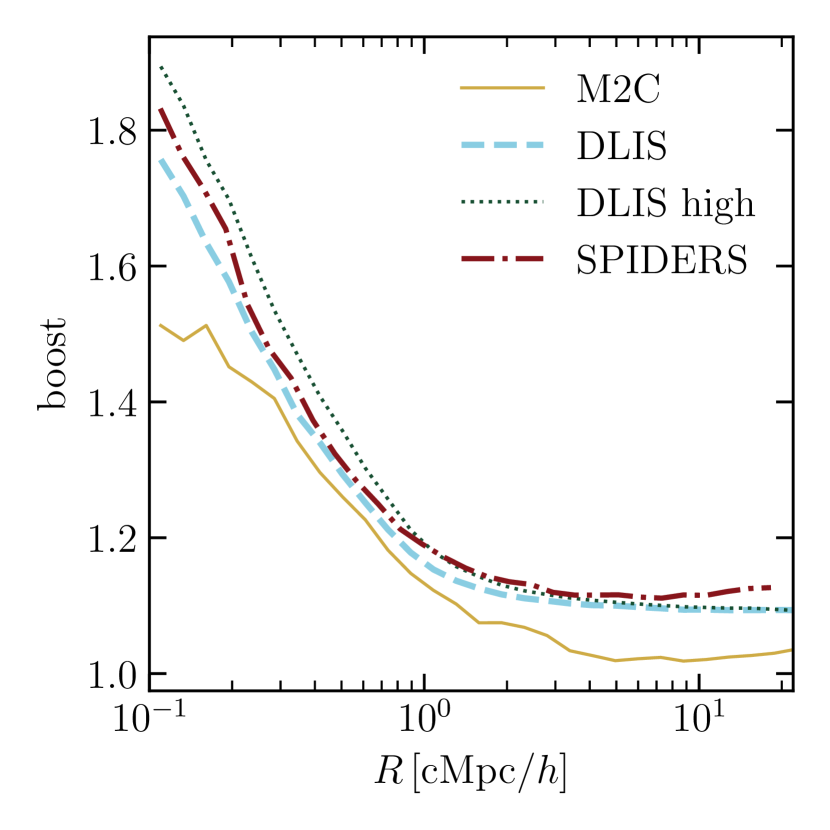
Figure 8: Boost factor calculated in dsigma for the observed $\Delta\Sigma$ profile (with $\Omega_{\rm m}=0.3$) of each publicly available cluster catalogue used in this work.

Appendix B Reduced shear approximation

In this work we assume the reduced shear is equal to the shear, ignoring a $1-\kappa$ correction. Here we justify that choice by estimating the size of $\kappa$ as a function of radius for the three cluster samples M2C, SPIDERS and DLIS high. The quantity to estimate is

$$\kappa=\frac{\Sigma(R)}{\Sigma_{\rm crit}}\,.$$ (20)

We can take $\Sigma_{\rm crit}$ from the lensing calculation, using the average value over all lenses in the sample. The $\Sigma(R)$ profile found when creating the matched simulation profiles in Fig. 2 is used. The result is seen in Fig. 9. We subtract the value at large $R$, which can not be known accurately due to the mass-sheet degeneracy, to find the contribution of the cluster over the background. The convergence correction drops below $20\%$ at $R=0.1\,$Mpc$/h$, where our fits to the profile begin, and is negligible in the infall region. We conclude that the reduced shear approximation is sufficient in our analysis.

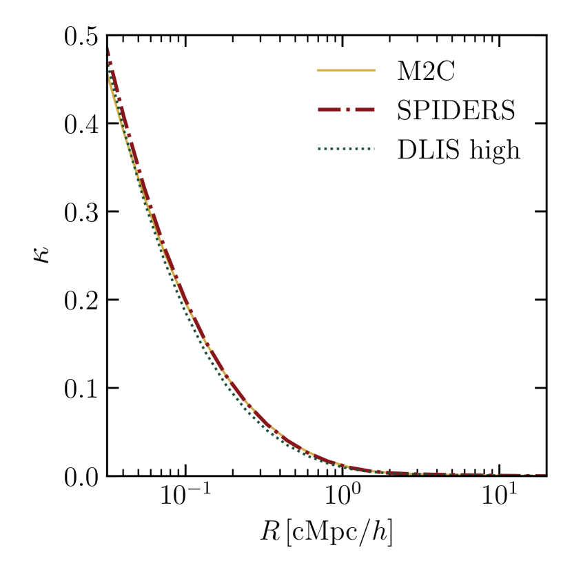
Figure 9: Convergence profiles for the three cluster catalogues used in this work. The constant value at large $R$ has been subtracted.

Appendix C Variation of splashback radius with assumed $\Omega_{\rm m}$

The assumed value of $\Omega_{\rm m}$ affects the resulting $\Delta\Sigma$ profile, as a cosmology must be assumed to convert from angles and redshifts into projected and line-of-sight distances. Here we test how this assumption impacts the location of $r_{\rm sp}$, as determined by the steepest slope of the density profile. For each choice of $\Omega_{\rm m}$, we rerun the full analysis pipeline. We find that the variation is within the uncertainty in all cases. However, for a robust analysis, both cosmology and the splashback radius should be jointly constrained from the data.

	$r_{\rm sp}\,$cMpc$\,h^{-1}$
Fiducial $\Omega_{\rm m}$	M2C	SPIDERS	DLIS high
$0.2$	$r_{\rm sp}=1.40^{+0.24}_{-0.16}$	$r_{\rm sp}=1.73^{+0.17}_{-0.15}$	$r_{\rm sp}=1.42^{+0.07}_{-0.06}$
$0.25$	$r_{\rm sp}=1.36^{+0.35}_{-0.19}$	$r_{\rm sp}=1.71^{+0.17}_{-0.14}$	$r_{\rm sp}=1.36^{+0.10}_{-0.09}$
$0.3$	$r_{\rm sp}=1.30^{+0.25}_{-0.13}$	$r_{\rm sp}=1.59^{+0.16}_{-0.13}$	$r_{\rm sp}=1.45^{+0.11}_{-0.11}$
$0.35$	$r_{\rm sp}=1.15^{+0.17}_{-0.11}$	$r_{\rm sp}=1.61^{+0.23}_{-0.15}$	$r_{\rm sp}=1.43^{+0.09}_{-0.09}$
$0.4$	$r_{\rm sp}=1.18^{+0.26}_{-0.17}$	$r_{\rm sp}=1.54^{+0.12}_{-0.10}$	$r_{\rm sp}=1.36^{+0.25}_{-0.31}$

Table 4: When finding $\Delta\Sigma$ profiles from a combined galaxy cluster and weak lensing shape catalogue, a value for $\Omega_{\rm m}$ is needed to convert angles and redshifts to distances. Here we demonstrate the impact on the recovered splashback radius from this choice.

Appendix D Fixing density profile model parameters

Fig. 10 demonstrates that the fit results for the density profile are largely the same when the parameters $\log\alpha$ and $\log\delta_{\rm max}$ are fixed or left free, but posteriors from infall region parameters are reduced.

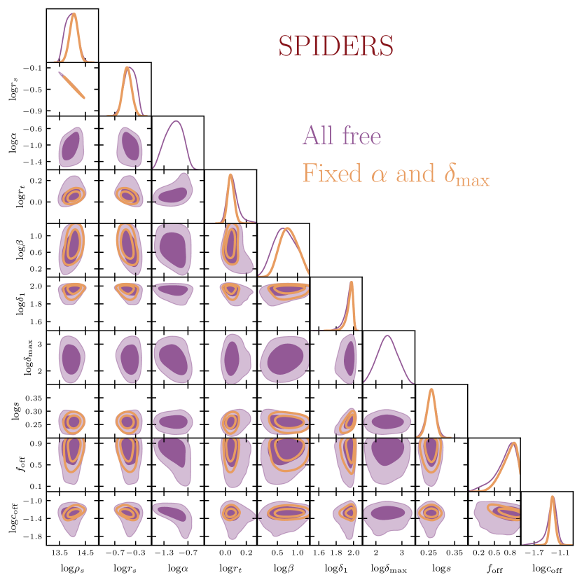
Figure 10: Comparison between best-fit parameters for the DLIS high profile (only using clusters with $M_{500{\rm c}}>10^{14}M_{\odot}/h$), when all parameters are left free, or $\alpha$ and $\delta_{\rm max}$ are kept fixed to their best fit values from the all free case.

References

- Amoura (2023) Amoura Y., 2023, PhD thesis, University of Waterloo
- Amoura et al. (2021) Amoura Y., Drakos N. E., Berrouet A., Taylor J. E., 2021, MNRAS, 508, 100
- Balmès et al. (2014) Balmès I., Rasera Y., Corasaniti P. S., Alimi J. M., 2014, MNRAS, 437, 2328
- Baxter et al. (2017) Baxter E., et al., 2017, Astrophys. J, 841, 18
- Bertin (2011) Bertin E., 2011, in Evans I. N., Accomazzi A., Mink D. J., Rots A. H., eds, Astronomical Society of the Pacific Conference Series Vol. 442, Astronomical Data Analysis Software and Systems XX. p. 435
- Bianconi et al. (2021) Bianconi M., Buscicchio R., Smith G. P., McGee S. L., Haines C. P., Finoguenov A., Babul A., 2021, Astrophys. J, 911, 136
- Blanton et al. (2017) Blanton M. R., et al., 2017, AJ, 154, 28
- Bleem et al. (2015) Bleem L. E., et al., 2015, ApJS, 216, 27
- Bleem et al. (2020) Bleem L. E., et al., 2020, ApJS, 247, 25
- Castro et al. (2021) Castro T., Borgani S., Dolag K., Marra V., Quartin M., Saro A., Sefusatti E., 2021, MNRAS, 500, 2316
- Diemer (2020) Diemer B., 2020, Astrophys. J. Suppl. Ser., 251, 17
- Diemer (2022) Diemer B., 2022, MNRAS, 519, 3292–3311
- Diemer (2024) Diemer B., 2024, A dynamics-based density profile for dark haloes – III. Parameter space (arXiv:2410.17324), https://arxiv.org/abs/2410.17324
- Diemer & Kravtsov (2014) Diemer B., Kravtsov A. V., 2014, Astrophys. J, 789, 1
- Diemer et al. (2017) Diemer B., Mansfield P., Kravtsov A. V., More S., 2017, Astrophys. J., 843, 140
- Dolag et al. (2004) Dolag K., Bartelmann M., Perrotta F., Baccigalupi C., Moscardini L., Meneghetti M., Tormen G., 2004, Astron. Astrophys., 416, 853
- Eckert et al. (2011) Eckert D., Molendi S., Paltani S., 2011, A&A, 526, A79
- Einasto (1965) Einasto J., 1965, Trudy Astrofizicheskogo Instituta Alma-Ata, 5, 87
- Euclid Collaboration et al. (2022) Euclid Collaboration et al., 2022, A&A, 662, A112
- Euclid Collaboration et al. (2024) Euclid Collaboration et al., 2024, arXiv e-prints, p. arXiv:2405.13491
- Farrens et al. (2022) Farrens S., et al., 2022, A&A, 664, A141
- Finoguenov et al. (2020) Finoguenov A., et al., 2020, A&A, 638, A114
- Fong & Han (2021) Fong M., Han J., 2021, MNRAS, 503, 4250
- Fukushige & Makino (2001) Fukushige T., Makino J., 2001, ApJ, 557, 533
- García et al. (2021) García R., Rozo E., Becker M. R., More S., 2021, MNRAS, 505, 1195
- Ghirardini et al. (2024) Ghirardini V., et al., 2024, A&A, 689, A298
- Gill et al. (2005) Gill S. P. D., Knebe A., Gibson B. K., 2005, MNRAS, 356, 1327
- Guerrini et al. (2024) Guerrini S., et al., 2024, arXiv e-prints, p. arXiv:2412.14666
- Guinot et al. (2022) Guinot A., et al., 2022, Astron. Astrophys., 666, A162
- Haggar et al. (2020) Haggar R., Gray M. E., Pearce F. R., Knebe A., Cui W., Mostoghiu R., Yepes G., 2020, MNRAS, 492, 6074
- Haggar et al. (2021) Haggar R., Pearce F. R., Gray M. E., Knebe A., Yepes G., 2021, MNRAS, 502, 1191–1204
- Haggar et al. (2024) Haggar R., Amoura Y., Mpetha C. T., Taylor J. E., Walker K., Power C., 2024, ApJ, 972, 28
- Hasselfield et al. (2013) Hasselfield M., et al., 2013, J. Cosmology Astropart. Phys., 2013, 008
- Heymans et al. (2012) Heymans C., et al., 2012, MNRAS, 427, 146
- Hildebrandt et al. (2012) Hildebrandt H., et al., 2012, MNRAS, 421, 2355
- Johnston et al. (2007) Johnston D. E., et al., 2007, arXiv e-prints, p. arXiv:0709.1159
- Karamanis et al. (2022a) Karamanis M., Nabergoj D., Beutler F., Peacock J. A., Seljak U., 2022a, arXiv preprint arXiv:2207.05660
- Karamanis et al. (2022b) Karamanis M., Beutler F., Peacock J. A., Nabergoj D., Seljak U., 2022b, Monthly Notices of the Royal Astronomical Society, 516, 1644
- Kirkpatrick et al. (2021) Kirkpatrick C. C., et al., 2021, MNRAS, 503, 5763
- Knollmann & Knebe (2009) Knollmann S. R., Knebe A., 2009, Astrophys. J. Suppl. Ser., 182, 608
- Lange & Huang (2022) Lange J., Huang S., 2022, dsigma: Galaxy-galaxy lensing Python package, Astrophysics Source Code Library, record ascl:2204.006
- Le Fèvre et al. (2005) Le Fèvre O., et al., 2005, A&A, 439, 845
- Lewis (2019) Lewis A., 2019, arXiv e-prints, p. arXiv:1910.13970
- Li et al. (2024) Li Q., et al., 2024, ApJ, 969, L25
- Liaudat et al. (2020) Liaudat T., Bonnin J., Starck J. L., Schmitz M. A., Guinot A., Kilbinger M., Gwyn S. D. J., 2020, arXiv e-prints, p. arXiv:2011.09835
- Maksimova et al. (2021) Maksimova N. A., Garrison L. H., Eisenstein D. J., Hadzhiyska B., Bose S., Satterthwaite T. P., 2021, MNRAS, 508, 4017
- Menanteau et al. (2010) Menanteau F., et al., 2010, ApJ, 723, 1523
- More et al. (2016) More S., et al., 2016, Astrophys. J, 825, 39
- Mpetha et al. (2024) Mpetha C. T., Taylor J. E., Amoura Y., Haggar R., 2024, MNRAS
- Navarro et al. (1996) Navarro J. F., Frenk C. S., White S. D. M., 1996, Astrophys. J, 462, 563
- Newman et al. (2013) Newman J. A., et al., 2013, ApJS, 208, 5
- O’Neil et al. (2021) O’Neil S., Barnes D. J., Vogelsberger M., Diemer B., 2021, MNRAS, 504, 4649
- Piffaretti et al. (2011) Piffaretti R., Arnaud M., Pratt G. W., Pointecouteau E., Melin J. B., 2011, A&A, 534, A109
- Planck Collaboration et al. (2011) Planck Collaboration et al., 2011, A&A, 536, A8
- Planck Collaboration et al. (2015) Planck Collaboration et al., 2015, A&A, 581, A14
- Planck Collaboration et al. (2016) Planck Collaboration et al., 2016, A&A, 594, A27
- Planck Collaboration et al. (2020) Planck Collaboration et al., 2020, Astron. Astrophys., 641, A6
- Rykoff et al. (2014) Rykoff E. S., et al., 2014, ApJ, 785, 104
- Sadibekova et al. (2024) Sadibekova T., Arnaud M., Pratt G. W., Tarrío P., Melin J. B., 2024, arXiv e-prints, p. arXiv:2402.01538
- Scodeggio et al. (2018) Scodeggio M., et al., 2018, A&A, 609, A84
- Shin & Diemer (2023) Shin T.-h., Diemer B., 2023, MNRAS, 521, 5570
- Singh et al. (2017) Singh S., Mandelbaum R., Seljak U., Slosar A., Vazquez Gonzalez J., 2017, MNRAS, 471, 3827–3844
- Smee et al. (2013) Smee S. A., et al., 2013, AJ, 146, 32
- Springel et al. (2021) Springel V., Pakmor R., Zier O., Reinecke M., 2021, MNRAS, 506, 2871
- Tarrío et al. (2019) Tarrío P., Melin J. B., Arnaud M., 2019, A&A, 626, A7
- Taylor (2005) Taylor M. B., 2005, in Shopbell P., Britton M., Ebert R., eds, Astronomical Society of the Pacific Conference Series Vol. 347, Astronomical Data Analysis Software and Systems XIV. p. 29
- Tomooka et al. (2020) Tomooka P., Rozo E., Wagoner E. L., Aung H., Nagai D., Safonova S., 2020, MNRAS, 499, 1291
- Towler et al. (2024) Towler I., et al., 2024, MNRAS, 529, 2017
- Unruh et al. (2020) Unruh S., Schneider P., Hilbert S., Simon P., Martin S., Puertas J. C., 2020, A&A, 638, A96
- Wen & Han (2024) Wen Z. L., Han J. L., 2024, ApJS, 272, 39
- Wright et al. (2020) Wright A. H., Hildebrandt H., van den Busch J. L., Heymans C., 2020, A&A, 637, A100
- Zürcher & More (2019) Zürcher D., More S., 2019, Astrophys. J, 874, 184
- van Daalen et al. (2011) van Daalen M. P., Schaye J., Booth C. M., Dalla Vecchia C., 2011, MNRAS, 415, 3649