Reducing real-time complexity via sub-control Lyapunov functions: from theory to experiments

Abstract

The techniques to design control Lyapunov functions (CLF), along with a proper stabilizing feedback, possibly in the presence of constraints, often provide control laws that are too complex for proper implementation online, especially when an optimization problem is involved. In this work, we show how to acquire an alternative, computationally attractive feedback. Given a nominal CLF and a nominal state feedback, we say that a different positive definite function is a Sub-control Lyapunov function (SCLF) if its Lyapunov derivative is negative-definite and bounded above by the Lyapunov derivative of the nominal function with the nominal control. It turns out that if we consider a family of basis functions, then a SCLF can be computed by linear programming, with an infinite number of constraints. The idea is that although the offline computational burden to achieve the new controller and solve the linear program is considerable, the online computational burden is drastically reduced. Comprehensive simulations and experiments on drone control are conducted to demonstrate the effectiveness of the study.

, , , ,

1 Introduction

The availability of powerful software packages for optimization [3, 38, 20], allows designing controllers with high performance. The clearest example is the ever-growing popularity of Model Predictive Control (MPC), where the stabilizing feedback policy is computed implicitly via an optimization problem, handling directly operating constraints and balancing between performance and actuator exploitation [8, 10]. Additional features, such as safety or robustness, can also be added by properly modifying the cost and constraints of the program [41, 43]. However, these sophisticated controllers often necessitate a large amount of processing power real-time, limiting their application to systems with ample computational capacity or slow dynamics.

To face this problem, in [6], an explicit expression of the optimal control is adopted as a look-up table, to be used online. However, its implementation becomes increasingly intractable with respect to the system’s dimensions and the length of the prediction horizon [27]. An alternative direction to attain online operability for these policies is to learn the implicit control law with machine learning using neural networks as a function approximator, such as in [11, 14, 31] or [26], to name a few. This synthesis can be viewed as a supervised learning problem where the feedback variables are the features labeled with the input decisions made by such an “expert” control. Although the strategy significantly reduces the computational footprint, there is still room for improvement in terms of fitting performance, theoretical guarantee, and training data characterization, especially when large-scale systems come into play [12, 15].

From a control theoretic viewpoint, stability can be ensured if there exists a control Lyapunov function (CLF) for the closed-loop dynamics. If successfully synthesized, the function provides a stability certificate, which can be exploited to derive efficient control laws, for instance adopting Sontag’s formula [36, 42] or a min-norm control [17].

A considerable effort has been devoted to synthesizing CLF. For instance, generally without any pre-constructed controller, piecewise continuous CLF can be numerically generated via solving a semi-definite program (SDP) [28] or a linear program (LP) [37, 25, 16, 34, 29]. For a complete survey on numerical methods for CLF synthesis, we refer to [18].

In this work, we assume that a CLF, $\Psi(x)$, and a feedback control $\omega(x)$, are available (possibly from optimal design) but that these functions are unsuitable for real-time implementation. The idea we pursue is that of replacing $\Psi(x)$ and $\omega(x)$ by a simpler $V(x)$, we call Sub-control Lyapunov function, along with a feedback $\bar{u}(x)$ amenable for real-time implementation.

Our solution is based on the parameterization of the CLF with a set of basis functions (see [19, 34, 13] and others). The non-positivity constraints of the function’s time derivative become linear with respect to the variable parameters. Since these conditions are imposed continuously over the state space, we need to cope with infinitely many constraints [24]. This approach was validated in our previous work [13], although the optimization problem was relaxed by randomly sampling the state space.

In this context of CLF computation, our goal is to provide a theoretical framework taking into account the performance of the deduced control. Specifically, we:

• formalize the concept of Sub-Control Lyapunov Functions (SCLF), which retains the optimal controller as possible feedback, but it also admits alternative low-cost feedback laws amenable for implementation;

• introduce a performance-based formulation to generate such an SCLF, describing a Semi-Infinite Linear Program (SILP) and propose an algorithm to solve the problem based on cutting-plane method;

• validate the proposed framework with illustrative examples and experimental tests.

In Section 3 we describe a computational approach to search for an SCLF via an SILP. Section 4 shows that the framework can be applied for nonlinear systems of non-trivial size with simulation studies. The method is also experimentally validated via a quadcopter control application. Section 5 concludes and discusses future work.

Notation: For $x,y\in\mathbb{R}^{n}$, $x_{i}$ is its $i$th entry, $|x|\leq|y|$ implies $|x_{i}|\leq|y_{i}|\ \forall i$ and $\|x\|$ denotes the Euclidean norm. With $x^{*}\in\mathbb{R}^{n}$, $\epsilon>0$, $\mathcal{B}_{\epsilon}(x^{*})\triangleq\{x\in\mathbb{R}^{n}:\|x-x^{*}\|\leq\epsilon\}$. The function $\underset{|u|\leq u_{max}}{\text{sat}(w)}$ returns the standard vector saturation with its $i$th component computed as $\max(\min(u_{i,max},w_{i}),-u_{i,max})$. For an integer $\ell$, $\mathcal{N}(\ell,a,b)$ denotes the set of $\ell$ real numbers evenly sampled in the interval $[a,b]$. $\mathrm{co}(\cdot)$ is the convex hull operator. diag$(\cdot)$ returns a block matrix with its entries diagonally arranged. All-ones vector is denoted as $\mathbf{1}$.

2 Sub-Control Lyapunov Functions

2.1 Definition and basic properties

Consider the system

$$\dot{x}=A(x)+B(x)u,\,\,u\in\mathcal{U},$$ (1)

with $x\in\mathbb{R}^{n},u\in\mathbb{R}^{m}$ denoting the state and input vector, respectively. $\mathcal{U}$ is the input constraint set. We consider the control problem of stabilizing the system at the equilibrium point $x=0,u=0$.

We call a control Lyapunov function (CLF), associated with the control $\omega(x):\mathbb{R}^{n}\rightarrow\mathcal{U}$, a locally Lipschitz positive definite function $\Psi(x):\mathbb{R}^{n}\rightarrow\mathbb{R}$ with the property:

$$D^{+}\Psi(x,\omega(x))+g(x,\omega(x))=0$$ (2)

where $g(x,u)$ is locally Lipschitz and positive for non-zero $(x,u)$, and where we have denoted by

$$D^{+}\Psi(x,\omega(x))$$ (3)

$$=\limsup_{h\rightarrow 0^{+}}\frac{\Psi(x+h(A(x)+B(x)\omega(x)))-\Psi(x)}{h},$$

the generalized directional derivative. In the smooth case of $\Psi(x)$, one clearly has:

$$D^{+}\Psi(x,\omega(x)) =\nabla\Psi(x)\left(A(x)+B(x)\omega(x)\right).$$ (4)

We consider the generalized derivative, since $\Psi(x)$ could be non-differentiable.

Note that function $g(x,u)$ having the property (2) can be associated with the performance index:

$$J(x(0),u(\cdot))=\int_{0}^{\infty}g(x(t),u(t))\mathrm{d}t$$ (5)

while $\Psi(x)$ is the cost–to–go function, solution of the Hamilton-Jacobi-Bellman equation:

$$\min_{u\in\mathcal{U}}\left[D^{+}\Psi(x,u)+g(x,u)\right]$$ (6)

$$=D^{+}\Psi(x,\omega(x))+g(x,\omega(x))=0$$

where we have denoted by $\omega(x)$ the minimizer control.

Finding $\Psi(x)$ and a an optimal control law $\omega(x)$, often requires brute force computation via numerical approaches, moreover they are often unsuitable for online implementation. To arrive at an approximation scheme, we introduce the following definition.

Definition 1.

Given a polynomially bounded nominal control Lyapunov function (CLF) $\Psi(x)$ equipped with the control $\omega(x)$ we say that the polynomially bounded positive definite function $V(x)$ is a global sub-control Lyapunov function (SCLF) of $\Psi(x)$, if

$$D^{+}V(x,\omega(x))\leq D^{+}\Psi(x,\omega(x))=-g(x,\omega(x)),~\forall x.$$ (7)

It is a local SCLF if the inequality holds for $V(x)\leq\kappa$, for some $\kappa>0$.

There is an important relation between $V(x)$ and $\Psi(x)$.

Proposition 1.

If $~V(x)$ is a SCLF of $~\Psi(x)$, then $V(x)\geq\Psi(x)$.

Let $x_{0}$ be an initial condition and consider the converging trajectory $\chi(t)$, such that $\chi(0)=x_{0}$, associated with the control $\omega(x)$. By integrating, we get

$$\begin{cases}V(x_{0})-V(\chi(\infty))=-\int_{0}^{\infty}~~D^{+}V(\chi(t),\omega(\chi(t)))\mathrm{d}t&\\ \Psi(x_{0})-\Psi(\chi(\infty))=-\int_{0}^{\infty}~~D^{+}\Psi(\chi(t),\omega(\chi(t)))\mathrm{d}t.&\end{cases}$$

As the control is stabilizing, $\chi(\infty)=0$. Hence, $V(x_{0})\geq\Psi(x_{0})$. Since $x_{0}$ is arbitrary, the claim follows. $\square$

In the sequel, for practical implementation, we consider smooth candidate SCLF.

2.2 Suboptimal control laws from SCLFs

Now we show how low-cost controllers can be associated with a smooth SCLF (with a performance loss). As can be seen from (2), by integrating with $x(0)=x_{0}$, one can write the optimal performance as:

$$J(x_{0},\omega(x))=-\int_{0}^{\infty}D^{+}\Psi(x,\omega(x))\mathrm{d}t=\Psi(x_{0}),$$ (8)

If the control $u=\omega(x)$ is unsuitable for real time implementation, we could replace $\Psi(x)$ by a smooth SCLF $V(x)$ defined as in (7), and adopt the following control:

$$\bar{u}(x)=\arg\min_{u\in\mathcal{U}}\nabla V(x)[A(x)+B(x)u]+g(x,u).$$ (9)

It is fundamental to note that problem (9) is feasible because $u=\omega(x)$, the optimal, is a feasible solution. The next theorem explains how this control performs.

Theorem 2.

Assume that the nominal $\Psi(x)$ satisfies (2). Consider a SCLF $V(x)$. Then control $\bar{u}(x)$ as in (9) is stabilizing. Moreover, given the cost function $g(x,u)$ and the initial condition $x(0)=x_{0}$, the performance is upper bounded by $V(x_{0})$.

We have that

$$\dot{V}(x,\bar{u}(x))+g(x,\bar{u}(x))=\nabla V(x)[A(x)+B(x)\bar{u}(x)]$$

$$+g(x,\bar{u}(x))\leq\underbrace{\nabla V(x)[A(x)+B(x)\omega(x)]}_{D^{+}V(x,\omega(x))}+g(x,\omega(x))$$

$$\leq D^{+}\Psi(x,\omega(x))+g(x,\omega(x))=0.$$

The first inequality is due to the fact that $\bar{u}(x)$ is the minimizer of the optimization problem (9), the second equality follows from the definition of a SCLF (7). Adopting the control $\bar{u}(x)$, the time derivative of $V(x)$ is

$$\dot{V}(x,\bar{u}(x))=\nabla V(x)[A(x)+B(x)\bar{u}(x)]\leq-g(x,\bar{u}(x)),$$ (10)

which implies asymptotic stability because $g(x,u)$ is positive definite, hence $V(\infty)=\underset{t\rightarrow\infty}{\lim}V(x(t))=0$. Then, integrating (10) leads to:

$$\int_{0}^{\infty}~~g(x,\bar{u}(x))\mathrm{d}t\leq V(x_{0})-V(\infty)=V(x_{0}).$$ (11)

$\square$

The computational complexity of the optimization problem (9) (to be solved in real-time), is very low and we can even provide a simple explicit solution in the case of a quadratic cost $g(x,u)$ and a box-type set $\mathcal{U}$ in (1).

Proposition 3.

Consider a quadratic cost:

$$g(x,u)=x^{\top}Qx+u^{\top}Ru,$$ (12)

with a positive definite diagonal weighting matrix $R=\text{diag}(r_{1},r_{2},...,r_{m})$ and a constraint set:

$$\mathcal{U}=\left\{u\in\mathbb{R}^{m}:|u|\leq u_{max}\right\}.$$ (13)

Then, the minimizer of (9) can be explicitly computed as:

$$\bar{u}(x)=\underset{|u|\leq u_{max}}{\text{sat}}\left(-\textstyle{\frac{1}{2}}R^{-1}B(x)^{\top}\nabla V(x)^{\top}\right)$$ (14)

Let $z=(\textstyle{\frac{1}{2}}\nabla V(x)B(x))^{\top}$ and $y=R^{-1}z$, then the problem (9) can be rewritten as:

$$\bar{u}(x)=\arg\min_{u\in\mathcal{U}}~2z^{\top}u+u^{\top}Ru,$$ (15)

$$=\arg\min_{u\in\mathcal{U}}~(u+y)^{\top}R(u+y)-y^{\top}Ry.$$

With the set $\mathcal{U}$ in (13), (15) is decoupled

$$\bar{u}(x)=\underset{|u|\leq u_{max}}{\arg\min}~\sum_{i=1}^{m}r_{i}(u_{i}+y_{i})^{2}.$$ (16)

For each component $\bar{u}_{i}(x)$ of $\bar{u}(x)$, the minimizer of (16) is: $\bar{u}_{i}(x)=\underset{|u_{i}|\leq u_{i,max}}{\text{sat}}(-y_{i}),$ or equivalently, (14). $\square$ For non-diagonal positive definite $R$, Proposition 3 does not hold. Still, one obtains a solution for the optimization problem as follows.

Proposition 4.

Let $u\in\mathcal{U}$ a polytope. Then problem (9) with cost (12), reduces to a minimum distance problem.

Denoting by $z=\frac{1}{2}\left(\nabla V(x)B(x)\right)^{\top}$, $\bar{u}(x)$ is the minimizer of

$$\bar{u}(x)=\mbox{arg}\min_{u\in\mathcal{U}}2z^{\top}u+u^{\top}Ru$$

Let $v=R^{\frac{1}{2}}u$ with $v\in\mathcal{V}\triangleq R^{\frac{1}{2}}\mathcal{U}$, the problem is equivalent, after completing the squares, to:

$$\begin{array}[]{l}\underset{v\in\mathcal{V}}{\min}\left\{-z^{\top}R^{-1}z+z^{\top}R^{-1}z+2z^{\top}R^{-\frac{1}{2}}v+v^{\top}v\right\}\\ =\underset{v\in\mathcal{V}}{\min}\left\{-z^{\top}R^{-1}z+\left(R^{-\frac{1}{2}}z+v\right)^{\top}\left(R^{-\frac{1}{2}}z+v)^{\top}\right)\right\}\\ =\min_{v\in\mathcal{V}}\left\{-z^{\top}R^{-1}z+\|R^{-\frac{1}{2}}z+v\|^{2}\right\}.\end{array}$$

So $v=R^{\frac{1}{2}}u$ is the point in $\mathcal{V}$ closest to $-R^{-\frac{1}{2}}z$. $\square$

Remark 5.

Solving the minimum distance problem is straightforward. Moreover, if $z(x)=\frac{1}{2}\left(\nabla V(x)B(x)\right)^{\top}$ is continuous, then the minimizer function $\bar{u}(x)$ is continuous as well being the so called minimal selection [4].

An essential property of a SCLF is that it admits, among other controllers the true optimal $\omega(x)$ beside the simpler $\bar{u}(x)$ discussed above. We expect that $\bar{u}(x)$ is close to $\omega(x)$. We argue that we can achieve optimality close to the origin. Indeed, assume a cost of the form (12) and the set of all control actions that ensure (10), or:

$$\nabla V(x)[A(x)+B(x)u]\leq-x^{\top}Qx-u^{\top}Ru,u\in\mathcal{U}.$$ (17)

Assume that, by means of linearization, we have determined an optimal desired gain $u=Kx$, the unconstrained local optimum, so that $\omega(x)\approx Kx$ close to $0$.

Parameterize the control as $u=Kx+v\in\mathcal{U}$. Complete the square and rewrite (17) as

$$Kx+v\in\mathcal{U}:\left\|R^{\frac{1}{2}}\left[v+Kx+\frac{1}{2}R^{-1}B(x)^{\top}\nabla V(x)^{\top}\right]\right\|^{2}$$

$$\leq-x^{\top}Qx-\nabla V(x)A(x)+\left\|\frac{1}{2}R^{-\frac{1}{2}}B(x)^{\top}\nabla V(x)^{\top}\right\|^{2}.$$ (18)

By construction, (17) and (18) are always feasible. Hence, we can compute the control as

$$\min\|v\|~\text{s.t.}~~~Kx+v\in\mathcal{U},\text{ and }\eqref{ineqquad}$$ (19)

which is, again, a straightforward minimum norm problem with quadratic and linear constraints. Since we assume that $\omega(x)\approx Kx$, and that $\omega(x)$ is a feasible control, in a neighborhood of $0$ we have the minimizer $v=0$ so that this new control will be virtually identical to $\omega(x)$.

2.3 Performance loss evaluation

Replacing $\Psi(x)$ by a SCLF $V(x)\geq\Psi(x)$ (by Proposition 1) entails a performance loss which can be quantified by the index:

$$\mbox{loss}=\frac{V(x_{0})}{\Psi(x_{0})}\geq 1.$$ (20)

Computing this index requires determining $\Psi(x)$ and $\omega(x)$, to impose the condition $D^{+}V(x,\omega(x))\leq D^{+}\Psi(x,\omega(x))=-g(x,\omega(x))$ to find $V(x)$ as we will see later. In practice, computing $\Psi(x)$, $D^{+}\Psi(x,\omega(x))$ explicitly and solving the $HJB$ optimality equation are affected by numerical and even non–differentiability issues [5]. Instead of solving the HJB equations, we can evaluate $\Psi(x)$ and $\omega(x)$ in (2) implicitly, by considering the problem:

$$\Psi(x_{0}) =\Psi_{\infty}(x_{0})= \inf_{u(\cdot)\in\mathcal{U}}\int_{0}^{\infty}g(x(\tau),u(\tau))\mathtt{d}\tau$$ (21a)

$$\dot{x}=A(x)+B(x)u,\quad$$ (21b)

$$x(0)=x_{0}.\quad\quad\quad\quad\;\;\,$$ (21c)

The control $\omega(x_{0})$ is the initial control value of the open-loop problem (21a)–(21c). Solving the infinite horizon problem (21a)–(21c) exactly may be difficult and, in practice, one has to approximate it by a finite (large) horizon problem [1]:

$$\Psi_{T}(x_{0})=\min_{u(\cdot)}{\int_{0}^{T}}g(x(\tau),u(\tau))\mathtt{d}\tau+\Phi(x(T)),$$ (22a)

$$\quad\quad\quad\dot{x}=A(x)+B(x)u,$$ (22b)

$$\quad\quad\quad u(\tau)\in\mathcal{U},\tau\in[0,T],$$ (22c)

$$\quad\quad\quad x(0)=x_{0},$$ (22d)

$$\quad\quad\quad x(T)\in\mathcal{P},$$ (22e)

where $T$ is the prediction horizon. $\mathcal{P}$ and $\Phi(\cdot)$ denote the controlled invariant terminal region and terminal cost function, respectively.

We now borrow ideas from Chen and Allgower [10], to evaluate the infinite-time performance. Let us consider the following assumption.

Assumption 1.

The terminal cost $\Phi(x)$ is smooth, positive definite and satisfies the HJB-like inequality

$$\min_{u\in\mathcal{U}}\{\dot{\Phi}(x,u)+g(x,u)\}$$

$$=\min_{u\in\mathcal{U}}\left\{\nabla\Phi(x)[A(x)+B(x)u]+g(x,u)\right\}\leq 0$$ (23)

in the terminal set $\mathcal{P}=\{x:\Phi(x)\leq\kappa$ }.

Remark 6.

For locally linearizable systems with the quadratic cost (12), we can take $\Phi(x)=x^{\top}Sx$. Then $\Phi(x)$ is a solution to (23) if $S$ satisfies the Riccati inequality

$$\bar{A}^{\top}S+S\bar{A}-S\bar{B}R^{-1}\bar{B}^{\top}S+Q\leq 0$$

where $\bar{A},\bar{B}$ are from the Jacobian linearization of (1) at $x=0,u=0$. The value $\kappa>0$ should be small enough so that (23) remains valid in $\mathcal{P}=\{x:x^{\top}Sx\leq\kappa\}$ [10].

Then we have the following result.

Theorem 7.

Under Assumption 1 consider the finite horizon model predictive scheme (22). This problem is recursively feasible. Assume that the optimal control $\omega(x)$ is continuous and denote by $\Psi_{T}(x)$ its value function. We have

$$D^{+}\Psi_{T}(x,\omega(x))\leq-g(x,\omega(x)),$$ (24)

hence $\Psi_{T}(x_{0})$ is a bound for the infinite time performance with $x(0)=x_{0}$, i.e.,

$$\int_{0}^{\infty}~g(x,\omega(x))\mathrm{d}t\leq\Psi_{T}(x_{0}).$$ (25)

We have that the region $\mathcal{P}$ is controlled invariant and that if we consider the minimizing control $u^{*}$ in (23), for $x_{0}\in\mathcal{P}$, by integrating, we get:

$$\int_{0}^{\infty}~g(x,u^{*})\mathrm{d}t\leq\Phi(x_{0}).$$

This means that the infinite-horizon open loop optimal cost with initial condition $x_{0}\in\mathcal{P}$ is upper bounded by $\Phi(x_{0})$. Recursive feasibility then follows from [10].

Take any initial $x(t)=x_{t}$ and denote by $\bar{u}_{t}$ and $\bar{x}_{t}$ the optimal solution on interval $[t,t+T]$. Consider a shifted interval $[\tau,\tau+T]$, with $t<\tau$ and take the difference

$$\Delta=\Psi_{T}(x(\tau))-\Psi_{T}(x(t))$$

$$=\min_{u}\left\{\int_{\tau}^{\tau+T}\hskip-11.38109ptg(x(\sigma),u(\sigma))\mathrm{d}\sigma+\Phi(x(\tau+T))\right\}$$

$$~~~-\min_{u}\left\{\int_{t}^{t+T}\hskip-11.38109ptg(x(\sigma),u(\sigma))\mathrm{d}\sigma+\Phi(x(t+T))\right\}$$

$$=\min_{u}\left\{\int_{\tau}^{\tau+T}\hskip-11.38109ptg(x(\sigma),u(\sigma))\mathrm{d}\sigma+\Phi(x(\tau+T))\right\}$$

$$~~~-\left\{\int_{t}^{t+T}\hskip-11.38109ptg(\bar{x}_{t}(\sigma),\bar{u}_{t}(\sigma))\mathrm{d}\sigma+\Phi(\bar{x}_{t}(t+T))\right\}.$$ (26)

Now we consider the solution $\bar{u}_{t}$ and $\bar{x}_{t}$ in the intersection interval $[\tau,t+T]$ in the first term, so achieving an inequality, and eliminate the common term $\int_{\tau}^{t+T}\hskip-8.53581ptg(\bar{x},\bar{u})\mathrm{d}\sigma$

$$\Delta\leq\min_{u}\left\{\int_{\tau}^{t+T}\hskip-11.38109ptg(x(\sigma),u(\sigma))\mathrm{d}\sigma\right.$$

$$~~~+\left.\int_{t+T}^{\tau+T}\hskip-11.38109ptg(x(\sigma),u(\sigma))\mathrm{d}\sigma+\Phi(x(\tau+T))\right\}$$

$$~~~-\left\{\int_{t}^{t+T}\hskip-11.38109ptg(\bar{x}_{t}(\sigma),\bar{u}_{t}(\sigma))\mathrm{d}\sigma+\Phi(\bar{x}_{t}(t+T))\right\}$$

$$=\min_{u}\left\{\int_{t+T}^{\tau+T}\hskip-11.38109ptg(x(\sigma),u(\sigma))\mathrm{d}\sigma+\Phi(x(\tau+T))\right\}$$ (27)

$$-\int_{t}^{\tau}g(\bar{x}_{t}(\sigma),\bar{u}_{t}(\sigma))\mathrm{d}\sigma-\Phi(\bar{x}_{t}(t+T))$$

$$=\underbrace{\min_{u}\int_{t+T}^{\tau+T}\hskip-14.22636ptg(x(\sigma),u(\sigma))\mathrm{d}\sigma+\Phi(x(\tau+T))-\Phi(\bar{x}_{t}(t+T))}_{\leq 0}$$

$$-\int_{t}^{\tau}g(\bar{x}_{t}(\sigma),\bar{u}_{t}(\sigma))\mathrm{d}\sigma\leq-\int_{t}^{\tau}g(\bar{x}_{t}(\sigma),\bar{u}_{t}(\sigma))\mathrm{d}\sigma.$$

The non–positivity of the term, follows by considering the initial state $\bar{x}_{t}(t+T)\in\mathcal{P}$ and integrating (23) in Assumption 1, bearing in mind that $x(\sigma)\in\mathcal{P}$ if $\sigma\in[t+T,\tau+T]$.

Now we need only to reconsider $\Delta$ divide by $\tau-t$ and take the limit $\tau-t\rightarrow 0$

$$D^{+}\Psi_{T}(x(t),\omega(x(t)))=\limsup_{\tau-t\rightarrow 0}\frac{\Psi_{T}(x(\tau))-\Psi_{T}(x(t))}{\tau-t}$$

$$=\limsup_{\tau-t\rightarrow 0}\frac{-1}{\tau-t}\int_{t}^{\tau}\hskip-2.84526ptg(\bar{x}_{t}(\sigma),\bar{u}_{t}(\sigma))\mathrm{d}\sigma$$

$$\leq-g(x(t),\omega(x(t))).$$ (28)

$\square$

Remark 8.

We have that (25) is not an equality as (6). However, for $T$ large enough and $\mathcal{P}$ small, there is no essential difference between the infinite and finite horizon performance, namely $\Psi(x)\approx\Psi_{T}(x)$, and (25) becomes close to an equality and roughly, $D^{+}\Psi(x,\omega(x))\approx-g(x,\omega(x))$. Hence, to search for an SCLF in practice, we will impose the condition $D^{+}V(x,\omega(x))\leq-g(x,\omega(x))$ rather than $D^{+}V(x,\omega(x))\leq D^{+}\Psi(x,\omega(x))$ to avoid computing $D^{+}\Psi(x,\omega(x))$.

3 Computation of a Sub-Control Lyapunov
Function

In this section, given a suitable setup, the computation of a SCLF will be cast into semi-infinite linear programming (SILP), i.e., a linear program with infinitely many constraints [37, 25, 19, 34]. Two procedures to solve such a problem will be discussed with different levels of complexity and efficiency.

One key point of the procedure is that we do not need to have the function $\Psi(x)$ to derive a sub-control Lyapunov function. We need just an algorithm to evaluate the optimal control $\omega(x)$ function and the given performance function $g(x,\omega(x))$ for off–line synthesis.

3.1 Finding an SCLF with SILP

Herein, under the standing assumption that the baseline control $\omega(x)$ is off-line computable, the construction of the SCLF can be carried out as follows. First, consider an SCLF candidate of the form:

$$V(x)=\sum_{k=1}^{N}\alpha_{k}V_{k}(x),$$ (29)

where $V_{k}(x),\alpha_{k}\geq 0$ are smooth positive definite functions and the corresponding coefficients. Then, consider the following program:

$${\alpha}^{*}= \arg\min_{\alpha\geq 0}\,\mathbf{1}^{\top}\alpha,$$ (30a)

$$\Omega({\alpha},x)\leq 0,$$ (30b)

$$x\in\mathcal{X}\subset\mathbb{R}^{n}.$$ (30c)

where ${\alpha}=[\alpha_{1},...,\alpha_{N}]^{\top}$ collects the coefficients $\alpha_{k}$ in (29), $\mathcal{X}$ is a compact region of interest containing the origin in its interior. $\Omega(\alpha,x):\mathbb{R}^{N}\times\mathbb{R}^{n}\rightarrow\mathbb{R}$ denotes the condition function:

$$\Omega({\alpha},x)\triangleq\dot{V}(x,\omega(x))+g(x,\omega(x))$$ (31)

$$=\nabla V(x)(A(x)+B(x)\omega(x))+g(x,\omega(x))$$

$$=\sum_{k=1}^{N}\alpha_{k}\nabla V_{k}(x)(A(x)+B(x)\omega(x))+g(x,\omega(x)).$$

The program (30) is a linear program with $N$ variables $\alpha_{k}$ and infinitely many linear constraints of the form (30b) with $x$ taken from $\mathcal{X}$. This leads to a so-called SILP which is a convex optimization problem and has been deeply investigated in the literature [2, 39, 22, 32]. By solving (30), one can obtain the following result.

Proposition 9.

If the semi-infinite linear program (30) has a feasible solution $\bar{\alpha}=[\bar{\alpha}_{1},...,\bar{\alpha}_{N}]^{\top}$, then $V(x)=\sum_{k=1}^{N}\bar{\alpha}_{k}V_{k}(x)$ is an SCLF.

The proof follows immediately by the satisfaction of (30b)–(30c) and Definition 1.

Remark 10.

The choice of $\textbf{1}^{\top}\alpha=\sum_{i}\alpha_{i}$ as cost in the linear program aims at finding the smallest value of $V(x)$ which is a CLF, to ensure the best performance (Theorem 2). Assume that $x_{0}$ is a nominal initial condition, representing a nominal perturbation. Then, as an alternative possibility, one can replace the cost function by $\sum_{i}\alpha_{i}V_{i}(x_{0})$, to specifically improve the performance from this state.

3.2 Discretization-based solution

To compute a feasible solution for (30), one direct approach is to sample or discretize the set $\mathcal{X}$ into a sufficiently dense grid of points $\mathcal{X}_{g}\subset\mathcal{X}$. Then, a candidate coefficient $\alpha$ can be found by solving (30a)–(30b) for $x\in\mathcal{X}_{g}$, making the optimization a standard Linear Program (LP):

$$\alpha^{*}=\underset{\alpha\geq 0}{\arg\min\,}\mathbf{1}^{\top}\alpha\text{ s.t. }\alpha\in\underset{x\in\mathcal{X}_{g}}{\bigcap}\{\alpha:\Omega(\alpha,x)\leq 0\}.$$ (32)

An immediate follow-up question would be how dense the grid $\mathcal{X}_{g}$ should be to obtain an acceptable solution within a certain range of tolerance for the constraints in (30). To address this concern, let us proceed with the following setup. Given a finite set $\mathcal{X}_{g}\subset\mathcal{X}$, define a granularity function:

$$\rho(x)=\underset{x_{g}\in\mathcal{X}_{g}}{\inf}\|x-x_{g}\|.$$ (33)

It is further assumed that the time derivative of $V(x)$ driven by the control $\omega(x)$ and the corresponding penalty $g(x,\omega(x))$ is Lipschitz continuous. Namely,

$$|\Gamma(x_{a})-\Gamma(x_{b})|\leq\nu\|x_{a}-x_{b}\|$$ (34)

$$|g(x_{a},\omega(x_{a}))-g(x_{b},\omega(x_{b}))|\leq\eta\|x_{a}-x_{b}\|,$$

with $x_{a},x_{b}\in\mathcal{X}$ and for brevity, we use the notation $\Gamma(x)\triangleq\dot{V}(x,\omega(x))=\nabla V(x)(A(x)+B(x)\omega(x))$.

Then we have the following proposition.

Proposition 11.

Suppose that we have a candidate $V(x)$ defined as in (29) by solving (32) for a finite set $\mathcal{X}_{g}\subset\mathcal{X}$. Namely, $\Omega(\alpha,x_{g})\leq 0~\forall x_{g}\in\mathcal{X}_{g}$, or,

$$\Gamma(x_{g})\leq-g(x_{g},\omega(x_{g}))~\forall x_{g}\in\mathcal{X}_{g}.$$ (35)

Then, given $0<\varphi<1,\exists\zeta(\varphi)>0$:

$$\Gamma(x)\leq-\varphi g(x,\omega(x)),$$ (36)

$\forall x\in\mathcal{X}\cap\{x:g(x,\omega(x))\geq\zeta(\varphi)\},$ and $\zeta(\varphi)\triangleq(\eta+\nu)\bar{\rho}/(1-\varphi)$, $\bar{\rho}=\sup_{x\in\mathcal{X}}\rho(x)$.

Consider $x\in\mathcal{X}$, $x_{g}\in\mathcal{X}_{g}\cap\mathcal{B}_{\bar{\rho}}(x)$, we have:

$$\Gamma(x)=\Gamma(x_{g})+\Gamma(x)-\Gamma(x_{g})$$ (37)

$$\leq-g(x_{g},\omega(x_{g}))+\nu\|x-x_{g}\|$$

$$=-g(x,\omega(x))+g(x,\omega(x))-g(x_{g},\omega(x_{g}))$$

$$\;\;\;\;\;\;\;\;\;\;\;\;\;\;\;\;\;\;\;\;\;\;\;\;\;\;\;\;\;\;\;\;\;\;\;\;\;\;\;\;\;\;\;\;\;\;\;\;\;\;\;\;\;+\nu\|x-x_{g}\|$$

$$\leq-g(x,\omega(x))+\eta\|x-x_{g}\|+\nu\|x-x_{g}\|$$

$$\leq-g(x,\omega(x))+(\eta+\nu)\bar{\rho}$$

$$\leq-\varphi g(x,\omega(x)),$$

where the last inequality follows from (36). $\square$ This is to say, if an accuracy $0<\varphi<1$ is selected (possibly close to $1$), the inequality (36) is guaranteed continuously outside the set $\{x:g(x,\omega(x))\leq\zeta(\varphi)\}$. The volume of this level set can be shrunken by squeezing $\bar{\rho}$, or increasing the density of the grid $\mathcal{X}_{g}$. Proposition 11 hence provides a theoretical analysis on the relation between the discretization of the continuous set $\mathcal{X}$ and the the characteristic parameters. However, although programmatically simple for low-dimensional systems, for high-dimensional systems, uniformly gridding the set $\mathcal{X}$ and solving (32) are not practical since the required number of points in $\mathcal{X}_{g}$ may grow aggressively with respect to the state dimension $n$. For this reason, in the following, as opposed to a fixed grid as in [24, 13], we establish an iterative procedure for suitably refining the set $\mathcal{X}_{g}$ based on the cutting-plane technique.

3.3 Cutting-plane-based solution

In this part, the cutting-plane (CP) method is employed to provide an iterative procedure for grid adaptation. The intuition is that of iteratively enforcing the constraint (30b) at the state where it is most violated [34]. Namely, in the variable space of $\alpha$, linear constraints (a.k.a., cuts) are added correspondingly. In this work, the CP technique is chosen, since in the optimization problem (30), there is only one continuous constraint described by (30b)–(30c). Hence, the violation can be evaluated by checking the non-positivity of the scalar function $\Omega(\alpha,x)$ in (31) over the domain $\mathcal{X}$ for a given candidate $\alpha$ resulted from (32), i.e., verifying:

$$\Omega^{*}=\Omega(\alpha,x^{*})\leq 0,$$ (38a)

with $$x^{*}=\arg\max_{x\in\mathcal{X}}\Omega(\alpha,x).$$ (38b)

Input: A compact set $\mathcal{X}$, a set of basis functions $V_{k}(x)$, and the control law $\omega(x)$.

Output: the SCLF $V(x)$.

1: Select an initial finite grid $\mathcal{X}_{g}\subset\mathcal{X}$;

2: Solve the LP (32) with $\mathcal{X}_{g}$ to get $\alpha$;

3: Define the function $V(x)$ as in (29);

4: Define $\Omega(\alpha,x)$ as in (31);

5: Compute $x^{*}$ and $\Omega^{*}$ as in (38);

6: if $\Omega^{*}>0$

7:    Append $\{x^{*}\}$ to the the grid points $\mathcal{X}_{g}$;

8:    go to step 2;

9: else

10:   return $V(x)$;

Algorithm 1 SCLF construction with CP method

If the certificate (38a) does not hold, $x^{*}$ in found (38b) is the point where the constraint $\Omega(\alpha,x)\leq 0$ (30b) is violated the most. This point will then be appended to the current grid $\mathcal{X}_{g}$ and the procedure will be reinitialized with such an updated grid. Concisely, Algorithm 1 summarizes the main steps of the SCLF construction based on CP technique, an illustrative flow chart is also provided in Fig. 1.

Remark 12.

Solving (38b) is not straightforward because the optimization problem is almost never convex. However, note that one has the non-convexity only in the state space $x$ when solving (38b). Therefore, even though non-trivial, with proper solvers, the algorithm can be applied for practical scenarios (see later in Section 4). Meanwhile, in the coefficient space $\alpha$ of high dimension, the problem is a standard LP in (32).

In the following part, to proceed with the construction of the SCLF for the numerical examples, we particularize the choice of the $\omega(x)$ and the basis functions $V_{k}(x)$.

3.4 Discussion

Figure 1: Procedure for the SCLF construction based on cutting-plane technique.

i) The ideal control $\omega(x)$:

To obtain a control law of optimal performance, among practical control strategies, quasi-infinite-horizon MPC [10] will be chosen as the software for generating stable closed-loop trajectories due to its standardized synthesis procedure.

For numerical implementation of the software, the constraint (22b) is approximated via the Euler discretization [8] with a sampling parameter $\tau_{s}>0$.

The next fundamental component will be the set of basis functions parameterizing the SCLF. In order to provide a rationale for our selection of such a set for the numerical examples, a brief review will be presented subsequently.

ii) The basis functions $V_{k}(x)$ choice

In the literature, the parameterization of the form (29) to find a CLF has been intensively studied. Hence, there are several options for the choice of the basis functions $V_{k}(x)$. Generally, this is often a trade-off between their flexibility and computational complexity in both offline synthesis and online deployment stages. For example, in the context of artificially generated CLF, one customary choice is a set of piecewise-affine (PWA) functions, making the synthesis abridge to an LP, accompanied by generalized analytical and practical guarantees [35, 19, 37]. Yet, if the processing power is limited, one encounters the problem of dimensionality again while dividing the state space into partitions (e.g., triangulations) during the offline phase. Meanwhile, the online phase faces the so-called point location problem when PWA functions are employed in the form of look-up tables. In the context of stability analysis for autonomous systems, a more complete set was used in [24] in the form of a Gaussian basis. This can be thought of as an interpolation of smooth quadratic functions, with the weight matrices being the decision variables, resulting in, again, an SILP. In this manner, the problem of imposing continuity on the function was also sidestepped. However, with this interpolation, the basis is again defined over a set of discrete knots, complicating the online applications with respect to the system’s size. Hence, depending on the computational power at hand, different choices of basis can be combined to acquire a satisfactory characterization. With these analyses, in view of maintaining smoothness, avoiding discretization-based interpolation, and taking advantage of the results for linear systems in [7, 13], we examine the set of basis functions composed as follows.

Let us first include in the basis a quadratic function:

$$V_{1}(x)=x^{\top}Px,$$ (39)

with the weight $P\succ 0$ computed from the algebraic Riccati equation for the linearly approximated dynamics of (1) around the origin. In this manner, we ensure that, around a neighborhood of the origin, we obtain some local optimality with the resulting function.

Next, the set of basis functions will be populated with $2p$-norm-like polynomial [7]:

$$V_{k}(x)=(a_{k}^{\top}x)^{2p},$$ (40)

where the function is characterized by the choice of the vector $a_{k}\in\mathbb{R}^{n}$. With this setting, by simply collecting $a_{k}$ with different directions and lengths, we can effectively expand the set of basis functions to achieve more representational capacity. An illustration in $\mathbb{R}^{2}$ is given in Fig. 2.

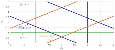
Figure 2: Unit level set of some basis functions of the form (40) and a linear combination of them (red), with $x\in\mathbb{R}^{2},p=2$.

With the characterization of $V_{k}(x)$ in (39)–(40), the idea is to increase the completeness of the basis with a possibly large number of basis (i.e., $N$ in (29)). This is the expense of fixing a priori the structure (shape and value) of the basis, as in (40). Yet, it will be shown later in the examples that, eventually, after the generation of the SCLF, there exist many basis functions associated with insignificantly small coefficients. Hence, in practice, those components of the parameterization can be discarded. In the numerical examples, a threshold $\varepsilon_{N}\ll 1$ will be defined so that only the coefficients $\alpha_{k}\geq\varepsilon_{N}$ are kept. The number of those remaining functions with will be denoted as $\underline{N}$. These functions will then be retained for the online control via (9).

So far, all the ingredients for the control synthesis with an SCLF are ready. Next, numerical examples will be provided with both simulation and experimental results, showing that the approach can be applied to non-trivial cases.

4 Numerical examples and experimental
validation

Herein, three systems will be examined to illustrate and showcase the effectiveness of the proposed machinery. First, the dynamics investigated will be recapitulated, and then the numerical results will be reported. Note that in the next part, without further explanation, the notation $x,u$ will be abused to denote the state and input vector of the system under discussion.

4.1 System description

Let us proceed by briefly summarizing the three control problems employed, as follows.

i) Bioreactor process (Bioreactor)

For the sake of illustration, we first examine a two-dimensional system of a bioreactor process governed by the following nonlinear dynamics [9, 33]:

$$\dot{x}_{1}=-(C_{1S}+x_{1})(1+u)+$$ (41)

$$~~~~D_{aS}(1-x_{2}-C_{2S})e^{(C_{2S}+x_{2})/\gamma}(C_{1S}+x_{1})$$

$$\dot{x}_{2}=-(C_{2S}+x_{2})(1+u)+$$

$$D_{aS}(1-x_{2}-C_{2S})e^{(C_{2S}+x_{2})/\gamma}\frac{(1+\beta)(C_{1S}+x_{1})}{1+\beta-x_{2}-C_{2S}}.$$

with the parameters $\gamma=0.4,\beta=0.02,D_{aS}=1.2$, $C_{1S}=0.0938,C_{2S}=0.9155.$ $x_{1}$ and $x_{2}$ denote the deviation from the equilibrium dedimensionalized states, while the dimensionless flow rate $u$ is the system’s input and its amplitude is constrained as:

$$|u|\leq u_{max}=1.$$ (42)

The control objective for system (41) is to stabilize $x_{1},x_{2}$ towards the origin. The domain of interest is set as $\mathcal{X}=\{x:|x|\leq 0.1\}$. With this model, it is important to note that the state, the input and even the time clock have been normalized. However, for consistency, the same notations for the variables and their derivatives will be used. For the technical analysis of the model construction, we would like to send the readers to [9, 33] and the references therein.

ii) Planar vertical take-off and landing aircraft (VTOL)

Next, to showcase the effectiveness of the technique over a non-trivial size system, we examine the normalized model of a vertical take-off and landing (VTOL) aircraft driven by the following dynamics [21, 30]:

$$\ddot{\xi}_{1} =-f_{1}\sin\xi_{3}+f_{2}\varepsilon\cos\xi_{3},$$ (43)

$$\ddot{\xi}_{2} =f_{1}\cos\xi_{3}+f_{2}\varepsilon\sin\xi_{3}-1,$$

$$\ddot{\xi}_{3} =f_{2},$$

where in (43), $\xi_{1},\xi_{2}$ and $\xi_{3}$ denote the 2-D positions of the aircraft’s center of mass and its roll angle, respectively. $\varepsilon=0.2$ is the system’s parameter, and “$-1$” represents the normalized gravitational acceleration. Finally, $f=[f_{1},\;f_{2}]^{\top}$ collects the thrust and rolling moment (see Fig. 3). The control objective here is to stabilize the system at the equilibrium point where:

$$\xi_{i}=0,\dot{\xi}_{i}=0,i\in\{1,2,3\},\text{ and }f=f_{e}=[1,\;0]^{\top}.$$ (44)

Figure 3: The planar VTOL model

To verify the SCLF found with the explicit control (14), the constraint on the input $f$ is intentionally chosen as:

$$[-2,\;-2]^{\top}\leq f\leq[4,\;2]^{\top}.$$ (45)

In this way, the error dynamics can be rewritten in the control affine form as:

$$\dot{x}_{1}=x_{2},\dot{x}_{2}=-(u_{1}+1)\sin x_{3}+u_{2}\varepsilon\cos x_{3},$$ (46)

$$\dot{x}_{3}=x_{4},\dot{x}_{4}=(u_{1}+1)\cos x_{3}+u_{2}\varepsilon\sin x_{3}-1,$$

$$\dot{x}_{5}=x_{6},\dot{x}_{6}=u_{2}.$$

with $x_{2i-1}=\xi_{i},i\in\{1,2,3\}$, while the input $u=f-f_{e}$ is restricted in the form of (13):

$$|u|\leq u_{max}=[3,\;2]^{\top}.$$ (47)

The investigated state space for this system is set as:

$$\mathcal{X}=\Big{\{}x:|x_{1}|,|x_{3}|\leq 1,|x_{2}|,|x_{4}|\leq 0.5,$$ (48)

$$\quad\quad\quad|x_{5}|\leq\pi/3,x_{6}\leq\pi/6\Big{\}}.$$

Table 1: Numerical parameters used in the SCLF synthesis and online control

	System & constraint	$Q$	$R$	$\tau_{s}$ (s)	$n_{g}$	$T^{\text{off}}$ (s)	$T^{\text{on}}$ (s)
Bioreactor	(41) and (42)	diag$(5,5)$	1	0.05	20	17.5	0.5
VTOL	(46) and (47)	diag$([5,1,5,1,10,1])$	diag$(4,4)$	0.05	1500	15	3.25
Drone	(53) and (54)	diag$([50,50,50,5,5,5])$	diag$(10,10)$	0.1	1500	12	3.5

iii) Quadcopter position control (Drone)

The final example will be the experimental validation for the position control (a.k.a., outer-loop control) of a nano-drone [13]. The dynamics can be given as follows:

$$\ddot{x}_{1}=F(\cos\phi\sin\theta\cos\psi+\sin\phi\sin\psi),$$ (49)

$$\ddot{x}_{2}=F(\cos\phi\sin\theta\sin\psi-\sin\phi\cos\psi),$$

$$\ddot{x}_{3}=-\underline{\mathsf{g}}+F\cos\phi\cos\theta,$$

where $x_{i},i={1,2,3}$ are the drone’s 3-D positions, $\underline{\mathsf{g}}$ is the gravitational acceleration. $(\phi,\theta,\psi)$ denote the roll, pitch, and yaw angles, respectively. $F\geq 0$ is the normalized thrust provided by the propellers. In this setting, $\psi$ is assumed to be known by measurement, while $F,\phi,\theta$ are the manipulated variables and constrained as:

$$0\leq F\leq\bar{F},|\phi|\leq\bar{\epsilon},|\theta|\leq\bar{\epsilon},$$ (50)

with $\bar{F}=1.45\underline{\mathsf{g}}$ and $\bar{\epsilon}=0.1745$ (rad) being the bounds of the thrust and the angles. These signals are then provided to the built-in inner-loop which controls the propellers with a proper conversion. Details for this hierarchical setting can be found in [23]. Then, the objective is to stabilize the drone at the equilibrium point, where:

$$x_{i}=0,\dot{x}_{i}=0,F=\underline{\mathsf{g}},\phi=\theta=0.$$ (51)

For that purpose, it was known that (49) can be exactly linearized via the input transformation:

$$F =\sqrt{u_{1}^{2}+u_{2}^{2}+(u_{3}+\underline{\mathsf{g}})^{2}},$$ (52a)

$$\phi =\arcsin{\left({(u_{1}\sin{\psi}-u_{2}\cos{\psi})}/{F}\right)},$$ (52b)

$$\theta =\arctan{\left({(u_{1}\cos{\psi}+u_{2}\sin{\psi})}/{(u_{3}+\underline{\mathsf{g}})}\right)}.$$ (52c)

Figure 4: Hierarchical control scheme of the experiments.

Indeed, replacing (52) in (49) yields:

$$\dot{x}_{i}=x_{i+3},\dot{x}_{i+3}=u_{i},i\in\{1,2,3\},$$ (53)

and the constraint (50) propagated through the mapping (52) can be under-approximated by the polytope [13]:

$$\mathcal{U}=\mathrm{co}\left\{\begin{aligned} [0,0,-\underline{\mathsf{g}}]^{\top},[r^{\star}\cos\mu,r^{\star}\sin\mu,u_{3}^{\star}]^{\top}&\\ [r\cos\mu,r\sin\mu,\sqrt{\bar{F}^{2}-r^{2}}-\underline{\mathsf{g}}]^{\top}&\end{aligned}\right\},$$ (54)

with $r^{\star}=\bar{F}\sin\bar{\epsilon}$, $u_{3}^{\star}=\bar{F}\cos\bar{\epsilon}-\underline{\mathsf{g}}$ and for some integers $S_{1},S_{2}>2$, $\mu\in\mathcal{N}(S_{1},0,2\pi),r\in\mathcal{N}(S_{2},0,r^{\star})$. For this work, we chose $S_{1}=8,S_{2}=2.$

In brief, the control problem now involves the stabilization of system (53) subject to $u=[u_{1},u_{2},u_{3}]^{\top}\in\mathcal{U}$ as in (54). The studied domain is chosen as:

$$\mathcal{X}=\{x:|x|\leq 1.5\}.$$ (55)

The complete scheme for this application is depicted in Fig. 4. Later, for this system, the experiments will be carried out on the Crazyflie 2.1 nano-drone in an indoor environment. Feedback signals will be estimated with the Qualisys motion capture system. For brevity, we would like to send the readers to our previous experiments in [13] for further details on the experimental platform. In short, the three systems and their constraints are summarized in the first two columns of Table 1.

4.2 Numerical results and discussion

In this part, the numerical results for the offline synthesis of the SCLF will be reported first. Subsequently, the applicability of the constructed SCLF will be demonstrated via simulations and experiments in comparison with the quasi-infinite-horizon MPC.

i) Offline synthesis for SCLFs

The offline construction will be carried out with the control software $\omega(x)$ calculated with the routine (22). For this setup, the cost function $g(x,u)$ will be chosen in the quadratic form as in (12). The corresponding terminal cost and constraints ($\Phi(x)$ and $\mathcal{P}$) therein will be uniquely determined as the quadratic function from the linear quadratic regulator and its ellipsoidal level set computed for the approximated dynamics at the origin [10]. Furthermore, as this is an offline effort, the prediction horizon in (22) is preferably chosen to be relatively large and denoted as $T=T^{\text{off}}$. Note that the superscript “off” is to distinguish the value from the prediction horizon used later for online comparison. To start Algorithm 1, the initial grid was chosen as a set of $n_{g}$ random points in $\mathcal{X}$. All the aforementioned values are reported in Table 1. All the receding horizon routines and quadratic programs will be solved with IPOPT software [40] via CasADi interface [3]. To evaluate the certificate (38), fmincon solver of MATLAB 2021b will be used with the sequential quadratic programming (SQP) approach.

Table 2: Specifications and total build time (BT) for the three systems

Model	$n$	$m$	$\;\;\;N$ in (29)	$\varepsilon_{N}$	$\underline{N}$	Total BT (h)
Bioreactor	2	1	1303	$5\mathrm{e}{-7}$	6	3.144
VTOL	6	2	1627	$1\mathrm{e}{-5}$	29	22.59
Drone	6	3	2561	$6\mathrm{e}{-6}$	38	80.93

Regarding the results in Table 2, we recall that $N$ denotes the number of basis functions employed in the optimization (30). $\varepsilon_{N}$ is the chosen threshold below which all the coefficients $\alpha_{k}$ found will be discarded, leaving $\underline{N}$ functions parameterizing $V(x)$ as in (29). The total build time (BT) used for running Algorithm 1 is also reported therein. Fig. 5 the values of $\Omega^{*}$ in (38a) found (blue) and the corresponding build time (orange) to find them along the iteration steps of the algorithm.

Figure 5: Largest violation found and build time (BT) for Bioreactor, VTOL and Drone model (top to bottom, respectively).

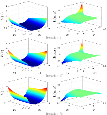
Figure 6: Snapshots of the SCLF candidates (left) and the verifier $\Omega(\alpha,{x})$ as in (31) (right) during the execution of Algorithm 1 for the bioreactor model (41).

Expectedly, the offline construction time grows with respect to the number of states and inputs. This can be explained by the search for $x^{*}$ in (38b) which requires a continuous evaluation of $\omega(x)$ within the SQP solver employed. It is also noticeable in Table 2 that, although using a large number of basis functions to find $V(x)$, the number of meaningful coefficients remaining is relatively small. This is, indeed, a positive sign, since later on, during the online implementation of (9), the calculation of $\nabla V(x)$ will require less computational power. Regarding the effectiveness of Algorithm 1, it can be seen from Fig. 5 and Table 1 that the total number of points in state space used to enforce the constraint (30b) is relatively small, in comparison with, for instance, a loose grid of 5 samples ($5^{n}$ points) in each axis.

Particularly for the Bioreactor model (41), the numerical result from Algorithm 1 is:

$$V(x)=1.957x^{\top}\begin{bmatrix}16.973&-0.147\\ -0.147&1.747\end{bmatrix}x+19.003([5,\,0]x)^{4}$$ (56)

$$+0.229([-2.823,\,4.127]x)^{4}+1.074([-3.141,\,3.890]x)^{4}$$

$$+0.833([-3.687,\,3.377]x)^{4}+9.003([-4.950,\,0.706]x)^{4}.$$

With this function, Fig. 5 and 6 also illustrate that the non-positivity of the surface $\Omega(\alpha,x)$ (i.e., the satisfaction of (30b)) is gradually enforced as Algorithm 1 goes through its steps, especially after the 17th iteration.

ii) Online control with the generated SCLFs

After achieving the function $V(x)$ from the offline stage, let us proceed by verifying the proposed control via simulations and experiments. The first performance indicator we would like to use is Theorem 2, or particularly the property in (10). With this inequality, we can show that the closed-loop system is asymptotically stable and verify the performance analysis in the theorem. For this reason, let us denote:

$$\Theta(x)\triangleq\dot{V}(x,\bar{u}(x))+g(x,\bar{u}(x))$$ (57)

$$=\nabla V(x)(A(x)+B(x)\bar{u}(x))+g(x,\bar{u}(x)),$$

the sum of the time derivative of $V(x)$ along the closed-loop trajectory driven by $u=\bar{u}(x)$ as in (9) and the corresponding cost function $g(x,u)$. Then, the system’s convergence can be shown via the non-positivity of $\Theta(x)$.

Figure 7: Closed-loop trajectories (blue) and the level set of the SCLF (dotted black) of the bioreactor model.

For the digital implementation, taking advantage of the input constraint’s shape, we employed the explicit control law in Proposition 3 for the Bioreactor and VTOL models. With a non-standard input constraint as in (54) for the Drone, during the experiments, the QP (9) was solved directly via IPOPT solver.

Figure 8: Planar VTOL stabilization with input constraints.

To highlight the computational advantage of the proposed control, for the same initial states, the routine (22) is considered for online control with the same choice of cost and constraints as in the offline synthesis part. The difference is only the horizon size, which is chosen as the minimum value of $T$ offering a feasible solution for the tested initial states. This value is denoted as $T^{\text{on}}$ and given in Table 1. Then, the root-mean-square error (RMSE) will be computed as in (58) to evaluate how the controls perform:

$$\text{RMSE}=\sqrt{\dfrac{1}{N_{s}}\sum_{k=1}^{N_{s}}\left\|x(kt_{s})\right\|^{2}}.$$ (58)

Fig. 7, 8 and 9 present the closed-loop trajectories with the stability indicator $\Theta(x)$ as in (57). Therein, it can be seen that with the SCLFs artificially generated before, the constrained systems are successfully stabilized, and the guarantee of $\Theta(x)\leq 0$ is also confirmed.

Table 3: Comparison between SCLF-induced controller and MPC

Model	SCLF		MPC
	CT (ms)	Avg. RMSE	CT (ms)	Avg. RMSE
Bioreactor	0.031	0.106	4.662	0.088
VTOL	0.207	0.706	22.174	0.6303
Drone	6.51	0.393	32.66	0.396

Figure 9: Experiments for the quadcopter position tracking with the generated SCLF.

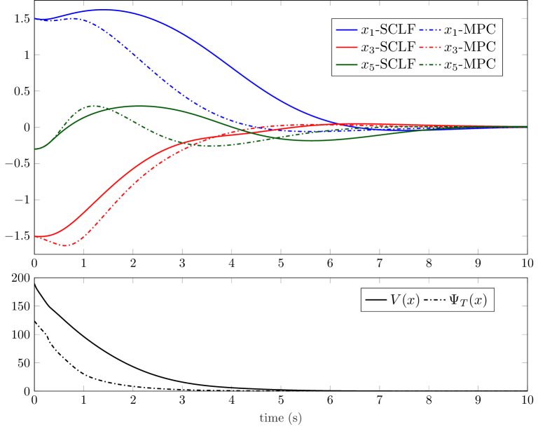
Figure 10: Suboptimal performance of the SCLF controller w.r.t. MPC in (22) for the VTOL model.

Regarding the performance, the trajectory of the VTOL from $x_{0}=[1.50,-0.19,-1.50,-0.17,-0.30,-0.02]^{\top}$ is reported in Fig. 10 for both the SCLF control (9) and MPC (22). The suboptimal transient behavior of the SCLF controller is evident through a larger rise time for the states. Additionally, interpreting the cost-to-go function’s upper bound, the SCLF $V(x)$ consistently exhibits a larger value compared to $\Psi_{T}(x)$ (22). To quantify the performance loss, we approximate the achievable cost of the infinite horizon formula (21) with Euler discretization of 1ms and 50s prediction horizon, yielding $\Psi_{\infty}(x_{0})\approx 62.96.$ Meanwhile, its upper bounds are given by the finite-horizon cost and the SCLF with $\Psi_{T}(x_{0})=123.55$ and $V(x_{0})=189.62$, gauging the trade-off to reduce implementation complexity. Indeed, although the proposed control deduced from the SCLFs showed slightly larger tracking error compared to the MPC law (22), its computational simplicity is a significant advantage. This simplicity is not only apparent with the explicit solution for the Bioreactor and VTOL, but also with the implicit law (9) for the Drone system, which requires significantly less computation time (CT) (See Table 3).

Finally, with the experiments on the Drone model, although satisfactory tracking is shown, one practical shortcoming of the proposed control (9) is revealed with the steady state error observed in Fig. 9. More specifically, there has not been any robustification measure taken into account in both offline and online phases. One possible direction is to incorporate the SCLF with an observer, compensating for the disturbance and uncertainty online.

5 Conclusion and outlook

This paper addresses a control problem for which there exists a controller of high performance but, at the same time, requiring excessive computational overhead. Our alternative solution centers around exploiting such an ideal control law to generate a stability certificate with suboptimal performance, called the Sub-Control Lyapunov Function (SCLF). With the SCLF, a more computationally low-cost control is derived, accompanied by an ancillary analysis of stability and suboptimality. Finally, a computational method is also provided to virtually generate the function based on the cutting-plane technique. The results are then successfully validated via both simulations and experiments on systems of non-trivial size and non-linearity. The future direction will focus on the robustification of the scheme, in not only the offline synthesis but also the online implementation, in conjunction with disturbance countermeasures.

This work is funded

References

- [1] M. Alamir. Stabilization of Nonlinear Systems Using Receding Horizon Technique. Lecture Notes in Control and Information Sciences, 339. Springer, Berlin, 2006.
- [2] Edward J Anderson and Peter Nash. Linear Programming in Infinite-dimensional Spaces: Theory and Applications. A Wiley-Interscience publication. Wiley, 1987.
- [3] Joel AE Andersson, Joris Gillis, Greg Horn, James B Rawlings, and Moritz Diehl. Casadi: a software framework for nonlinear optimization and optimal control. Mathematical Programming Computation, 11:1–36, 2019.
- [4] J. P. Aubin and A. Cellina. Differential inclusions, volume 264 of Grundlehren der Mathematischen Wissenschaften. Springer-Verlag, Berlin, 1984.
- [5] M. Bardi and I. Capuzzo Dolcetta. Optimal Control and Viscosity Solutions of Hamilton-Jacobi-Bellman Equations. Birkhäuser, Boston, 1997.
- [6] Alberto Bemporad, Manfred Morari, Vivek Dua, and Efstratios N Pistikopoulos. The explicit linear quadratic regulator for constrained systems. Automatica, 38(1), 2002.
- [7] Franco Blanchini and Stefano Miani. A new class of universal Lyapunov functions for the control of uncertain linear systems. IEEE Transactions on Automatic Control, 44(3):641–647, 1999.
- [8] Franco Blanchini, Stefano Miani, and Felice Andrea Pellegrino. Suboptimal receding horizon control for continuous-time systems. IEEE transactions on automatic control, 48(6):1081–1086, 2003.
- [9] David D Brengel and Warren D Seider. Multistep nonlinear predictive controller. Industrial & engineering chemistry research, 28(12):1812–1822, 1989.
- [10] Hong Chen and Frank Allgöwer. A quasi-infinite horizon nonlinear model predictive control scheme with guaranteed stability. Automatica, 34(10):1205–1217, 1998.
- [11] Steven Chen, Kelsey Saulnier, Nikolay Atanasov, Daniel D Lee, Vijay Kumar, George J Pappas, and Manfred Morari. Approximating explicit model predictive control using constrained neural networks. In 2018 Annual American control conference (ACC), pages 1520–1527. IEEE, 2018.
- [12] Steven W Chen, Tianyu Wang, Nikolay Atanasov, Vijay Kumar, and Manfred Morari. Large scale model predictive control with neural networks and primal active sets. Automatica, 135:109947, 2022.
- [13] Huu-Thinh Do, Franco Blanchini, Stefano Miani, and Ionela Prodan. LP-generated control Lyapunov functions with application to multicopter control. IEEE Transactions on Control Systems Technology, 32(6):2090–2101, 2024.
- [14] Ján Drgoňa, Karol Kiš, Aaron Tuor, Draguna Vrabie, and Martin Klaučo. Differentiable predictive control: Deep learning alternative to explicit model predictive control for unknown nonlinear systems. Journal of Process Control, 116:80–92, 2022.
- [15] Ján Drgoňa, Damien Picard, Michal Kvasnica, and Lieve Helsen. Approximate model predictive building control via machine learning. Applied energy, 218:199–216, 2018.
- [16] Mirko Fiacchini, Christophe Prieur, and Sophie Tarbouriech. On the computation of set-induced control Lyapunov functions for continuous-time systems. SIAM Journal on Control and Optimization, 53(3):1305–1327, 2015.
- [17] Randy A Freeman and Petar V Kokotovic. Inverse optimality in robust stabilization. SIAM journal on control and optimization, 34(4):1365–1391, 1996.
- [18] Peter Giesl and Sigurdur Hafstein. Review on computational methods for Lyapunov functions. Discrete and Continuous Dynamical Systems-B, 20(8):2291–2331, 2015.
- [19] Peter A Giesl and Sigurdur F Hafstein. Revised CPA method to compute Lyapunov functions for nonlinear systems. Journal of Mathematical Analysis and Applications, 410(1):292–306, 2014.
- [20] Michael Grant and Stephen Boyd. CVX: Matlab software for disciplined convex programming, version 2.1. https://cvxr.com/cvx, March 2014.
- [21] John Hauser, Shankar Sastry, and George Meyer. Nonlinear control design for slightly non-minimum phase systems: Application to V/STOL aircraft. Automatica, 28(4), 1992.
- [22] Rainer Hettich and Kenneth O Kortanek. Semi-infinite programming: theory, methods, and applications. SIAM review, 35(3):380–429, 1993.
- [23] Zipeng Huang, Robert Bauer, and Ya-Jun Pan. Closed-loop identification and real-time control of a micro quadcopter. IEEE Transactions on Industrial Electronics, 69(3):2855–2863, 2021.
- [24] Tor A Johansen. Computation of Lyapunov functions for smooth nonlinear systems using convex optimization. Automatica, 36(11):1617–1626, 2000.
- [25] Pedro Julian, Jose Guivant, and Alfredo Desages. A parametrization of piecewise linear Lyapunov functions via linear programming. International Journal of Control, 72(7-8):702–715, 1999.
- [26] Benjamin Karg and Sergio Lucia. Efficient representation and approximation of model predictive control laws via deep learning. IEEE Transactions on Cybernetics, 50(9), 2020.
- [27] Michal Kvasnica, Juraj Hledík, Ivana Rauová, and Miroslav Fikar. Complexity reduction of explicit model predictive control via separation. Automatica, 49(6):1776–1781, 2013.
- [28] Reza Lavaei and Leila J Bridgeman. Systematic, Lyapunov-based, safe and stabilizing controller synthesis for constrained nonlinear systems. IEEE Transactions on Automatic Control, 2023.
- [29] Mircea Lazar and Andrej Jokic. Synthesis of trajectory-dependent control Lyapunov functions by a single linear program. In International Workshop on Hybrid Systems: Computation and Control, pages 237–251. Springer, 2009.
- [30] Philippe Martin, Santosh Devasia, and Brad Paden. A different look at output tracking: Control of a vtol aircraft. Automatica, 32(1):101–107, 1996.
- [31] Sayak Mukherjee, Ján Drgoňa, Aaron Tuor, Mahantesh Halappanavar, and Draguna Vrabie. Neural Lyapunov differentiable predictive control. In 2022 IEEE 61st Conference on Decision and Control. IEEE, 2022.
- [32] Elijah Polak. Optimization: algorithms and consistent approximations, volume 124. Springer Science & Business Media, 2012.
- [33] S Ramaswamy, TJ Cutright, and HK Qammar. Control of a continuous bioreactor using model predictive control. Process Biochemistry, 40(8):2763–2770, 2005.
- [34] Hadi Ravanbakhsh and Sriram Sankaranarayanan. Learning control Lyapunov functions from counterexamples and demonstrations. Autonomous Robots, 43:275–307, 201.
- [35] Matteo Rubagotti, Luca Zaccarian, and Alberto Bemporad. A Lyapunov method for stability analysis of piecewise-affine systems over non-invariant domains. International Journal of Control, 89(5):950–959, 2016.
- [36] Eduardo D Sontag. A ‘universal’ construction of Artstein’s theorem on nonlinear stabilization. Systems & control letters, 13(2):117–123, 1989.
- [37] Tom Robert Vince Steentjes, Mircea Lazar, and Alina Ionela Doban. Construction of continuous and piecewise affine feedback stabilizers for nonlinear systems. IEEE Transactions on Automatic Control, 66(9):4059–4068, 2020.
- [38] Linas Stripinis and Remigijus Paulavičius. Directgo: A new direct-type matlab toolbox for derivative-free global optimization. ACM Transactions on Mathematical Software, 48(4):1–46, 2022.
- [39] Yoshihiro Tanaka, Masao Fukushima, and Toshihide Ibaraki. A comparative study of several semi-infinite nonlinear programming algorithms. European Journal of Operational Research, 36(1):92–100, 1988.
- [40] Andreas Wächter and Lorenz T Biegler. On the implementation of an interior-point filter line-search algorithm for large-scale nonlinear programming. Mathematical programming, 106:25–57, 2006.
- [41] Zhe Wu, Fahad Albalawi, Zhihao Zhang, Junfeng Zhang, Helen Durand, and Panagiotis D Christofides. Control Lyapunov-barrier function-based model predictive control of nonlinear systems. Automatica, 109:108508, 2019.
- [42] Yuh Yamashita, Ryosuke Matsukizono, and Koichi Kobayashi. Asymptotic stabilization of nonlinear systems with convex-polytope input constraints by continuous input. Automatica, 138:110032, 2022.
- [43] Jun Zeng, Bike Zhang, and Koushil Sreenath. Safety-critical model predictive control with discrete-time control barrier function. In 2021 American Control Conference (ACC), pages 3882–3889. IEEE, 2021.