Gradient Descent Converges Linearly to Flatter Minima
than Gradient Flow in Shallow Linear Networks

Abstract

We study the gradient descent (GD) dynamics of a depth-2 linear neural network with a single input and output. We show that GD converges at an explicit linear rate to a global minimum of the training loss, even with a large stepsize–about $2/\textrm{sharpness}$. It still converges for even larger stepsizes, but may do so very slowly. We also characterize the solution to which GD converges, which has lower norm and sharpness than the gradient flow solution. Our analysis reveals a trade off between the speed of convergence and the magnitude of implicit regularization. This sheds light on the benefits of training at the “Edge of Stability”, which induces additional regularization by delaying convergence and may have implications for training more complex models.

1 Introduction

Training modern machine learning (ML) models like deep neural networks via empirical risk minimization (ERM) requires solving difficult high-dimensional, non-convex, under-determined optimization problems. Although they are usually intractable to solve in theory, we train models effectively in practice using algorithms like stochastic gradient descent (SGD). This highlights a disconnect between the worst-case convergence rate of SGD and its convergence on specific ERM problems that arise from training, e.g., neural networks. Even if we can solve the ERM problem, typical minimizers of the under-determined objective will overfit and generalize poorly. That said, the specific solutions found by SGD and its variants usually do successfully generalize. Understanding how and why we are able to successfully optimize and generalize with these models is of great interest to the ML community and could help fuel continued progress in applied ML.

A key feature of popular ML models, including neural networks, is that the model output is related to the product of model parameters in successive layers. For instance, the output of a 2 layer feed-forward network with ReLU activations has output $\mathbf{W}_{2}\operatorname{\mathrm{ReLU}}(\mathbf{W}_{1}x+\mathbf{b}_{1})$, which is closely related to the product of the weight matrices $\mathbf{W}_{2}\mathbf{W}_{1}$. Ultimately, this “self-multiplication” of different model parameters gives rise to the non-convex and under-determined ERM problems that cause such (theoretical) difficulties.

In this work, we distill this parameter self-multiplication property down to its simplest form and comprehensively explain how it affects the training optimization dynamics, the “implicit regularization” of the model parameters, and the “edge-of-stability” dynamics that arise in certain regimes. In particular, we consider the extremely simple problem of learning a univariate linear model $\hat{y}=mx$ to minimize the squared error, except we parameterize the slope as $m=m(\mathbf{a},\mathbf{b})=\mathbf{a}^{\top}\mathbf{b}$ in terms of self-multiplying parameters $\mathbf{a},\mathbf{b}\in{\mathbb{R}}^{d}$. This can also be thought of as a depth-2 linear neural network with $d$ hidden units. For training data $\{(x_{i},y_{i})\in{\mathbb{R}}\times{\mathbb{R}}\}_{i=1}^{n}$, this results in the loss

$$\min_{\mathbf{a},\mathbf{b}\in{\mathbb{R}}^{d}}\bar{L}(\mathbf{a},\mathbf{b})\quad:=\quad\frac{1}{2n}\sum_{i=1}^{n}\left(\mathbf{a}^{\top}\mathbf{b}x_{i}-y_{i}\right)^{2}.$$ (1)

This objective is equivalent—by rescaling and subtracting a constant—to the even simpler loss

$$\min_{\mathbf{a},\mathbf{b}\in{\mathbb{R}}^{d}}L(\mathbf{a},\mathbf{b})\quad:=\quad\frac{1}{2}\left(\mathbf{a}^{\top}\mathbf{b}-\Phi\right)^{2}.$$ (2)

In what follows, we focus on this formulation and assume $\Phi\geq 0$ w.l.o.g. for simplicity and clarity.

Despite its simplicity, the objective (2), which has also been studied by prior work (Lewkowycz et al., 2020; Wang et al., 2022; Chen & Bruna, 2023; Ahn et al., 2024; Xu & Ziyin, 2024), is a useful object of study because it has a number of qualitative similarities to more complex and realistic problems like deep learning training objectives. First, it has similar high-level properties—the problem (2) is non-convex and highly under-determined because the set of minimizers constitutes the ($2d-1$)-dimensional hyperboloid in ${\mathbb{R}}^{2d}$ that solves $\mathbf{a}^{\top}\mathbf{b}=\Phi$. It also exhibits some of the same symmetries as realistic neural networks; for example, $\mathbf{a}^{\top}\mathbf{b}$ is invariant to swapping “neurons” $(\mathbf{a}_{i},\mathbf{b}_{i})\leftrightarrow(\mathbf{a}_{j},\mathbf{b}_{j})$ or to rescaling $(\mathbf{a}_{i},\mathbf{b}_{i})\to(c\mathbf{a}_{i},c^{-1}\mathbf{b}_{i})$. More importantly, the dynamics when optimizing (2) with gradient descent are qualitatively similar to the dynamics of training more complex models (see, e.g., Xu & Ziyin, 2024). Simultaneously, the problem (2) is simple enough that we can provide a detailed and nearly comprehensive characterization of several different aspects of training.

Main Contributions

We analyze the discrete (finite-step) gradient descent (GD) trajectories for the above objective and provide the following results:

1. Convergence of Gradient Descent.

Prior work (Wang et al., 2022) shows that GD converges to a global minimum from almost every initialization, despite the non-convexity of (2). We strengthen this claim by proving linear convergence despite no PL-condition: GD converges at a linear rate, with explicit dependence on the stepsize $\eta$, the initial parameters $(\mathbf{a}(0),\mathbf{b}(0))$, and the target value $\Phi$. Additionally, we identify several distinct phases in the training dynamics, determined by the relationships among the stepsize $\eta$, the parameter scale $\boldsymbol{\lambda}:=\|\mathbf{a}\|^{2}+\|\mathbf{b}\|^{2}$, and the residual $\boldsymbol{\varepsilon}:=\mathbf{a}^{\top}\mathbf{b}-\Phi$. Some of these phases align with the so-called Edge of Stability (EoS) phenomenon (Cohen et al., 2021), where GD continues to reduce the loss even when the Hessian’s largest eigenvalue exceeds $2/\eta$.

2. Location of Convergence.

Beyond convergence speed, we also describe which global minimizers GD selects out of the many solutions satisfying $\mathbf{a}^{\top}\mathbf{b}=\Phi$. We show that GD implicitly regularizes the imbalance

$$Q\;=\;\sum_{i=1}^{d}\bigl{|}\mathbf{a}_{i}^{2}-\mathbf{b}_{i}^{2}\bigr{|},$$

consistently decreasing $Q$ whenever $\eta$ is not too large, whereas gradient flow (GF) conserves $Q$. This discrepancy implies that discretizing the training steps (i.e., using GD) can produce strictly flatter solutions compared to GF—since the solution’s “sharpness,” or top Hessian eigenvalue, is tied to $\|\mathbf{a}\|^{2}+\|\mathbf{b}\|^{2}$. In particular, larger stepsizes promote stronger regularization and lower sharpness. While this sharper–flatter distinction has no effect on this model’s prediction (the function is the same at all global minima), it can be relevant for generalization in more complex settings (Hochreiter & Schmidhuber, 1997; Keskar et al., 2016; Smith & Le, 2018; Park et al., 2019). There is a large body of work, indeed, in other contexts showing that flatter minima of the loss tend to generalize better (Hochreiter & Schmidhuber, 1997; Keskar et al., 2016; Smith & Le, 2018; Park et al., 2019), and our analysis shows how the self-multiplying structure of (2) tends to regularize the sharpness.

Key Implications.

Overall, these findings yield a near-complete picture of how the “product-parameterized” objective $\tfrac{1}{2}\bigl{(}\mathbf{a}^{\top}\mathbf{b}-\Phi\bigr{)}^{2}$ behaves under GD. Beyond their intrinsic interest, we believe these results yield useful intuition for large-step training and implicit regularization for general neural networks. In particular,

1. GD Regularizes More Than GF.  On this model, discretized GD strictly reduces the parameter imbalance $Q$ (and thus the norm) beyond what continuous gradient flow achieves, with bigger step sizes regularizing more. However, $Q$ does not necessarily vanish to zero, so solutions are typically not maximally regularized.

2. GF Is Not Always a Good Proxy.  Since gradient flow preserves $Q$, while GD decreases it, using GF to approximate GD can be misleading—particularly at moderate or large $\eta$. Our results quantify such discrepancies.

3. Convergence Speed vs. Regularization Trade-off.  Surprisingly, stronger implicit regularization of $Q$ generally slows the overall convergence rate, and vice versa. This trade-off is closely linked to the EoS regime, where a large $\eta$ can flatten the final solution but may cause non-monotonic or slower convergence.

Technical Overview.

The key to our analysis is the following pair of observations. On the one hand, gradient descent iterations change the imbalance like $Q(t+1)=|1-\eta^{2}\boldsymbol{\varepsilon}(t)^{2}|Q(t)$, so the imbalance decreases throughout optimization for $0<\eta<\nicefrac{{\sqrt{2}}}{{\lvert\boldsymbol{\varepsilon}(t)\rvert}}$. At the same time, the objective $L$ does not globally satisfy the Polyak-Łojasiewicz (PL) condition (Polyak, 1963) because the origin is a saddle point, but it does satisfy a version of the PL condition along the GD trajectory, which is sufficient to prove linear convergence of GD to a global minimizer. Interestingly, the PL constant along the GD trajectory, which controls the speed of convergence, is equal to the smallest value of $\boldsymbol{\lambda}(t)$ encountered along the way, which is itself approximately equal to the value of $Q(t)$ at the first time that $\mathbf{a}(t)^{\top}\mathbf{b}(t)>0$. Thus, the stronger the implicit regularization of $Q$, the slower the convergence of GD, and vice versa, which puts these goals directly at odds.

2 Related Work

A large body of research has shown empirically that training neural networks with larger learning rates tends to lead to better generalization (LeCun et al., 2002; Bjorck et al., 2018; Li et al., 2019; Jastrzebski et al., 2020). However, in classical settings, convergence can only be guaranteed when the stepsize is small enough that $\boldsymbol{\lambda}_{\max}(\nabla^{2}L)<\nicefrac{{2}}{{\eta}}$ throughout optimization (Bottou et al., 2018). Nevertheless, a recent line of work starting with Cohen et al. (2021) observed that when training neural networks, the maximum eigenvalue of the Hessian, or “sharpness”, tends to grow throughout training until it reaches, or even surpasses the critical $\nicefrac{{2}}{{\eta}}$ threshold. But rather that diverging, the loss continues to decrease (non-monotonically) while the sharpness continues to hover around $\nicefrac{{2}}{{\eta}}$, which is referred to as the Edge of Stability (EoS) phenomenon. Understanding more deeply the training of neural networks with large stepsizes is of great interest.

Problems closely resembling (2) have been studied previously. Ahn et al. (2024) study losses of the form $\ell(ab)$ with $a,b\in{\mathbb{R}}$ and $\ell$ any convex, Lipschitz, and even function. The assumption that $\ell$ is even means it is minimized at zero (this is analogous to $\Phi=0$ in our case), and they prove convergence to zero from any initialization with any stepsize, but without a rate. However, this result relies crucially on both the loss being Lipschitz and minimized at zero. This is not surprising—we know that GD diverges on realistic objectives when the stepsize is too large. They also show that the limit point of gradient descent satisfies $\lvert a_{\infty}^{2}-b_{\infty}^{2}\rvert\approx\min\{\nicefrac{{2}}{{\eta}},\lvert a_{0}^{2}-b_{0}^{2}\rvert\}$, i.e. the imbalance between the weights is implicitly regularized down to the level of $\nicefrac{{2}}{{\eta}}$. Chen & Bruna (2023) study (2) with scalar $a,b\in{\mathbb{R}}$ and prove that the limit point of GD satisfies $a-b\to 0$ when the stepsize is chosen slightly too large for convergence to any minimizer $ab=\Phi$ to be possible. This is qualitatively similar to our work, but they intentionally choose a too-large stepsize in order to highlight the implicit regularization of the imbalance, while we provide conditions on $\eta$ under which convergence to a minimizer and some amount of regularization happen simultaneously.

In a related study, Xu & Ziyin (2024) explore the continuous dynamics of gradient flow using the exact same model discussed here. They demonstrate that the dynamics unfold along a one-dimensional curve, with the location of convergence distinctly defined by conserved quantities. Contrary to their findings, our research reveals this is not the case for gradient descent, highlighting the danger of relying excessively on continuous models to understand discrete non-convex optimization dynamics.

In the most closely related work, Wang et al. (2022) study the exact objective (2) and show that gradient descent using any stepsize up to $\eta\lesssim\nicefrac{{4}}{{\textrm{sharpness}}}$—approximately twice as large as the classical threshold of $\nicefrac{{2}}{{\textrm{sharpness}}}$—eventually converges to a minimizer, but without a rate. They also show some level of implicit regularization of $\boldsymbol{\lambda}$, e.g. at convergence $\boldsymbol{\lambda}\leq\frac{2}{\eta}$. In comparison, we provide an explicit convergence rate for GD and give a more detailed connection between this rate and the implicit regularization.

Finally, many papers have studied other models such as matrix factorization or linear neural networks (Saxe et al., 2014; Arora et al., 2019; Gidel et al., 2019; Tarmoun et al., 2021; Xu et al., 2023; Nguegnang et al., 2024), which are more faithful representations of realistic neural networks, but they are also much more difficult to analyze. Due to this difficulty, these results often only apply to gradient flow, or to GD with a very small learning rate, or to GD under additional, hard to interpret assumptions. In this work, we focus on the problem (2) in order to obtain a simpler, easier to interpret set of results.

3 Preliminaries

We study gradient descent (GD) on the quadratic loss

$$L(\mathbf{a},\mathbf{b})\;=\;\tfrac{1}{2}\,\bigl{(}\mathbf{a}^{\top}\mathbf{b}\;-\;\Phi\bigr{)}^{2},\quad\mathbf{a},\mathbf{b}\,\in\mathbb{R}^{d},$$ (3)

where $\Phi\geq 0$. The discrete updates take the form

$$\!\!\begin{bmatrix}\mathbf{a}(t+1)\\[2.0pt] \mathbf{b}(t+1)\end{bmatrix} =\,\begin{bmatrix}\mathbf{a}(t)\\[2.0pt] \mathbf{b}(t)\end{bmatrix}\,-\,\eta\nabla L\bigl{(}\mathbf{a}(t),\mathbf{b}(t)\bigr{)}$$

$$=\,\begin{bmatrix}\mathbf{a}(t)\\[2.0pt] \mathbf{b}(t)\end{bmatrix}\,-\,\eta\bigl{(}\mathbf{a}(t)^{\top}\mathbf{b}(t)-\Phi\bigr{)}\!\begin{bmatrix}\mathbf{b}(t)\\[2.0pt] \mathbf{a}(t)\end{bmatrix}\!,$$ (4)

but tracking the evolution of $\mathbf{a},\mathbf{b}$ directly can be unwieldy. Instead, we reparametrize via three auxiliary quantities that more cleanly describe the training dynamics.

Residuals.

Define the residual

$$\boldsymbol{\varepsilon}\;:=\;\mathbf{a}^{\top}\mathbf{b}\;-\;\Phi.$$

This scalar measures the distance to the manifold of global minima $\{\mathbf{a}^{\top}\mathbf{b}=\Phi\}$. Its sign and magnitude will be key to understanding convergence.

Norm of the parameters.

Let

$$\boldsymbol{\lambda}\;:=\;\|\mathbf{a}\|^{2}\;+\;\|\mathbf{b}\|^{2}.$$

Crucially, the Hessian of (3) at a point $(\mathbf{a},\mathbf{b})$ satisfying $\mathbf{a}^{\top}\mathbf{b}=\Phi$ is

$$\nabla^{2}L(\mathbf{a},\mathbf{b})\;=\;\begin{bmatrix}\mathbf{b}\\[2.0pt] \mathbf{a}\end{bmatrix}\!\begin{bmatrix}\mathbf{b}\\[2.0pt] \mathbf{a}\end{bmatrix}^{\top},$$ (5)

whose top eigenvalue (sharpness) is exactly $\boldsymbol{\lambda}$. In particular, the flattest possible minimizer has $\boldsymbol{\lambda}=2\Phi$, achieved when $\mathbf{a}$ and $\mathbf{b}$ coincide up to a sign (due to Cauchy-Schwarz inequality). Moreover, $\boldsymbol{\lambda}$ governs how the residuals evolve under (4). Indeed, we have that

$$\boldsymbol{\varepsilon}(t+1)\;=\;\boldsymbol{\varepsilon}(t)\,\Bigl{[}\,1\;-\;\eta\,\boldsymbol{\lambda}(t)\;+\;\eta^{2}\,\boldsymbol{\varepsilon}(t)\!\bigl{(}\boldsymbol{\varepsilon}(t)+\Phi\bigr{)}\Bigr{]}.$$ (6)

Hence, the term $-\,\eta\,\boldsymbol{\lambda}(t)$ is the principal driver for reducing $\boldsymbol{\varepsilon}(t)$. In turn, $\boldsymbol{\lambda}(t)$ evolution is governed by $\boldsymbol{\varepsilon}(t)$

$$\boldsymbol{\lambda}(t+1)\;=\;\bigl{[}\,1+\eta^{2}\,\boldsymbol{\varepsilon}(t)^{2}\bigr{]}\;\boldsymbol{\lambda}(t)\,-\,4\eta\boldsymbol{\varepsilon}(t)\bigl{(}\boldsymbol{\varepsilon}(t)+\Phi\bigr{)}.$$ (7)

The imbalance.

Finally, define $Q_{i}:=\mathbf{a}_{i}^{2}-\mathbf{b}_{i}^{2}$ for $i=1,\ldots,d$ and let

$$Q\;:=\;\sum_{i=1}^{d}\bigl{|}\,Q_{i}\,\bigr{|}.$$

This quantifies how “imbalanced” the individual components of $\mathbf{a}$ and $\mathbf{b}$ are. Under gradient flow, each $Q_{i}$ is conserved, but under discrete GD we have

$$Q_{i}(t+1) =\;\bigl{[}\,1\;-\;\eta^{2}\,\boldsymbol{\varepsilon}(t)^{2}\,\bigr{]}\;Q_{i}(t),$$ (8)

Whenever $\eta<\sqrt{2}\bigl{/}\!\bigl{|}\boldsymbol{\varepsilon}(t)\bigr{|}$, the term $\bigl{|}\,1-\eta^{2}\,\boldsymbol{\varepsilon}(t)^{2}\bigr{|}$ is in $(0,1)$, so $Q$ strictly decreases as $Q_{i}$, for all $i$, decreases in absolute value. This decline in $Q$ represents a core implicit regularization effect unique to discrete steps. Our analysis leverages $Q$ in two main ways: (i) lower-bounding $\boldsymbol{\lambda}$ by $Q$ to control convergence speed, and (ii) characterizing which minimizer (among the infinitely many) the algorithm ultimately selects.

Together, $\boldsymbol{\varepsilon}(t),\boldsymbol{\lambda}(t)$, and $Q(t)$ offer a more tractable viewpoint than tracking $\mathbf{a}(t)$ and $\mathbf{b}(t)$ directly. In subsequent sections, we use these reparametrized updates (6)–(8) to analyze both the speed of convergence and the location (norm/sharpness) of the solution.

4 Location of Convergence

We first address the question of which minimizers (among the infinitely many satisfying $\mathbf{a}^{\top}\mathbf{b}=\Phi$) is selected by GD. Our main theorem shows that GD reduces the imbalance $Q_{i}:=\mathbf{a}_{i}^{2}-\mathbf{b}_{i}^{2}$, whereas GF keeps it constant.

Theorem 1.

Let $0<\eta<\min\Bigl{\{}\tfrac{1}{2|\boldsymbol{\varepsilon}(0)|},\tfrac{2}{\sqrt{\boldsymbol{\lambda}(0)^{2}+4\,\Phi^{2}}}\Bigr{\}}.$ Then, at the limit point of gradient descent we have

$$\begin{split}&0\;<\;|Q_{i}(0)|\,\exp\Bigl{(}-\tfrac{\sqrt{\eta}\,\boldsymbol{\varepsilon}(0)^{2}}{\Phi}\Bigr{)}\;<\;|Q_{i}(\infty)|\quad\text{and}\\ &|Q_{i}(\infty)|\;<\;|Q_{i}(0)|\,\exp\Bigl{(}-\eta^{2}\!\sum_{t=0}^{\infty}\boldsymbol{\varepsilon}(t)^{2}\Bigr{)}\;<\;|Q_{i}(0)|,\end{split}$$

for all $i\in\{1,2,\ldots,d\}$.

The proof follows directly from iterating the update in Equation (8), which governs the evolution of each $Q_{i}$ under GD. The first bound on the step size is needed to prove the lower bound on $|Q_{i}(\infty)|$, and the second to show rapid convergence (cf. Theorem 2). A full proof is located in Appendix H.

Figure 1: Case for $\mathbf{a}=a,\mathbf{b}=b\in{\mathbb{R}}$. Under gradient flow, the trajectory curves away from the origin, conserving $Q_{i}$. GD’s discrete step moves along the affine tangent space, shrinking $Q_{i}$.

Figure 1 offers a geometric intuition: GF conserves the quantities $Q_{i}$ by curving away from the origin:

$$\dot{Q_{i}}=2(\mathbf{a}_{i}\,\dot{\mathbf{a}}_{i}-\mathbf{b}_{i}\,\dot{\mathbf{b}}_{i})=2\bigl{(}\mathbf{a}_{i}(-\,\boldsymbol{\varepsilon}\,\mathbf{b}_{i})-\mathbf{b}_{i}(-\,\boldsymbol{\varepsilon}\,\mathbf{a}_{i})\bigr{)}=0.$$

By contrast, the discretization error, introduced by the fact that gradient descent moves along the parallel vector to the curve, results in GD moving “inward” towards the line $\mathbf{a}=\mathbf{b}$, as illustrated by Figure 1. This results in smaller imbalances $Q_{i}$, although it never reduces them to exactly $0$ (unless there is a step where $\eta=1/\boldsymbol{\varepsilon}$ exactly).

Takeaway 1: GD converges to a solution with strictly lower imbalance than GF, though the imbalance never vanishes entirely.

Theorem 1 describes an implicit regularization effect which is only due to the action of discretizing the dynamics. Given that GF is frequently used as a simpler analytical stand-in for gradient descent in the literature, Takeaway 1 underscores the risks associated with over-relying on this approximation, potentially leading to inaccurate predictions about real-world behaviors.

Quantifying the Implicit Regularization.

From Equation (8) and Theorem 1, we can approximate $Q_{i}(\infty)$ when $\eta\,|\boldsymbol{\varepsilon}(t)|$ stays sufficiently small:

$$\begin{split}|Q_{i}(\infty)|&\;=\;|Q_{i}(0)|\cdot\prod_{t=0}^{\infty}\bigl{|}\,1-\eta^{2}\,\boldsymbol{\varepsilon}(t)^{2}\bigr{|}\\ &\;\approx\;|Q_{i}(0)|\cdot\exp\Bigl{(}-\,\eta^{2}\!\sum_{t=0}^{\infty}\boldsymbol{\varepsilon}(t)^{2}\Bigr{)}.\end{split}$$ (9)

Hence, $Q_{i}(\infty)$ depends directly on how quickly $\boldsymbol{\varepsilon}(t)$ (and thus the loss) decreases. In Section 5, we show that under certain step-size conditions, $\boldsymbol{\varepsilon}(t)$ converges linearly, implying $\sum_{t=0}^{\infty}\boldsymbol{\varepsilon}(t)^{2}\,\approx\,\frac{\boldsymbol{\varepsilon}(0)^{2}}{\eta\,\mu},$ so the final imbalance $Q(\infty)$ experiences only a modest reduction. Conversely, in slower convergence regimes, $\sum_{t=0}^{\infty}\boldsymbol{\varepsilon}(t)^{2}$ can be very large, making $Q(\infty)$ significantly smaller than $Q(0)$. Thus, slower optimization can result in stronger regularization.

5 Speed of Convergence

While Wang et al. (2022) already showed that gradient descent (GD) converges for this model initialized almost everywhere, we now establish an explicit rate of convergence to a global minimizer. We also establish in Proposition 1 the exponential convergence of GF for every initialization.

Theorem 2.

Let

$$0<\eta<\min\!\Bigl{\{}\tfrac{1}{2\,|\boldsymbol{\varepsilon}(0)|},\;\tfrac{2}{\sqrt{\boldsymbol{\lambda}(0)^{2}+4\,\Phi^{2}}}\Bigr{\}},$$

and define

$$\bar{\eta}\;:=\;\min\Bigl{\{}\,\eta,\;\tfrac{2}{\sqrt{\boldsymbol{\lambda}(0)^{2}+4\,\Phi^{2}}}-\eta\Bigr{\}}.$$

Assume $Q(0)\neq 0.$ Then for any $\delta>0$, there exists an iteration $T$ such that $L\bigl{(}\mathbf{a}(T),\mathbf{b}(T)\bigr{)}\leq\delta$, and

$$T \;\leq\;\mathcal{O}\bigg{(}\frac{\log(\mathbf{a}(0)^{\top}\mathbf{b}(0))}{\eta\Phi}+\frac{|\mathbf{a}(0)^{\top}\mathbf{b}(0)|}{\eta\Phi}$$ (10)

$$\quad+\;\frac{\log\!\bigl{(}\tfrac{1}{\delta}\bigr{)}}{\bar{\eta}\,Q(0)\,\exp\bigl{(}\min\{-\,\mathbf{a}(0)^{\top}\mathbf{b}(0),\,0\}\bigr{)}+\bar{\eta}\,\Phi}\biggr{)}.$$ (11)

If instead

$$\min\Bigl{\{}\tfrac{\sqrt{2}}{|\boldsymbol{\varepsilon}|},\;\tfrac{2}{\sqrt{\boldsymbol{\lambda}(0)^{2}+4\,\Phi^{2}}}\Bigr{\}}\;<\;\eta\;<\;\min\Bigl{\{}\tfrac{2}{|\boldsymbol{\varepsilon}|},\;\tfrac{2}{\boldsymbol{\lambda}}+\tfrac{2\,\boldsymbol{\varepsilon}\,(\boldsymbol{\varepsilon}+\Phi)}{\boldsymbol{\lambda}^{3}}\Bigr{\}},$$

then GD converges but may do so at a logarithmically slow rate.

A detailed proof appears in Appendix E-F, while Section 6 sketches the main ideas. The theorem shows that even when $\eta$ is relatively large (but below certain thresholds), GD converges linearly, up to a constant additive term reflecting how long it takes to escape the region around its initialization. Concretely, the convergence can be split into two phases:

• Equation (10): A phase where $|\boldsymbol{\varepsilon}|>|\Phi|$, during which convergence may slow and the trajectory risks nearing the saddle at the origin, although with probability 1 it avoids it, generally very quickly. We show that the speed of escaping of this phase is exponential up to log factors.

• Equation (11): A phase where the iterates are sufficiently close to the manifold of minima ($\mathbf{a}^{\top}\mathbf{b}\approx\Phi$), yielding exponential convergence once the dynamics remains in regions A and B (see below). This is the setting in which theorems of convergence of linear networks as the one in (Arora et al., 2019) apply.

Hence, the overall convergence speed is exponential. It is important to note that the rate of convergence in both phases depends on the unbalance $Q$ at the iteration in which we switch phase. This implies that if $Q$ is smaller, convergence happens slower. At the same time, in the previous section we established that if convergence is slower then the implicit regularization on $Q$ is stronger. This unveils an important trade off in the dynamics:

Takeaway 2: Stronger implicit regularization in the first phase of the training slows convergence. Generally, faster speed of training slows implicit regularization and slower speed of convergence imply stronger implicit regularization.

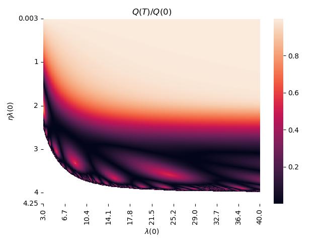
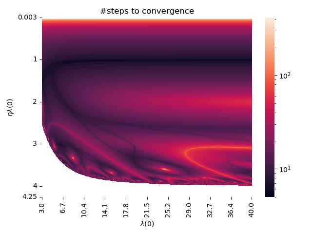
Figure 3: Gradient descent on (2) with $\Phi=1$ and various step sizes and initial scales. Left: Ratio $Q(T)/Q(0)$ showing how little $Q$ changes when $\eta\,\boldsymbol{\lambda}(0)$ is small and how strongly it is reduced for large $\eta\,\boldsymbol{\lambda}(0)$. Right: The time to converge to a small residual, illustrating slower convergence in cases with stronger $Q$-regularization. The chaotic behavior appears when $\eta\geq 1/\boldsymbol{\varepsilon}$.

This speed–regularization trade-off is illustrated in Figure 3. Even then, we observe an inverse relationship between speed and the strength of $Q$-regularization.

Edge-of-Stability Case

Recent work (Cohen et al., 2021) on training neural networks with MSE shows that for full-batch gradient descent, the Hessian’s largest eigenvalue generally hovers just above $2/\eta$ without causing divergence. For linear gradients, $\eta>\tfrac{2}{\boldsymbol{\lambda}}$ ordinarily implies divergence (e.g., the 1D parabola case), yet real neural networks manage to converge. The model we analyze offers a possible explanation: the product structure, combined with discrete updates, still allows convergence for $\eta>\tfrac{2}{\boldsymbol{\lambda}}$, but more slowly.

Moreover, our work hint to a possible important and surprising benefit of training at the Edge of Stability: we prove that the slower the convergence and the larger $\eta$, the smaller the inbalance $Q$. Hence, training at the edge of stability albeit at the cost of longer or more oscillatory paths, may enhance implicit regularization,.

6 Proof Sketch

In what follows we present informally the proof of Theorem 2. Note that Equation (6) implies approximately that

$$\boldsymbol{\varepsilon}(t+1)\approx(1-\eta\boldsymbol{\lambda}(t))\boldsymbol{\varepsilon}(t).$$ (12)

We show in Appendix C that if at initialization $\eta<\tfrac{2}{\sqrt{\boldsymbol{\lambda}(0)^{2}+4\,\Phi^{2}}}$ this will be the case throughout the trajectory. This implies that $\eta\boldsymbol{\lambda}(t)$ is upper bounded by a quantity strictly smaller than 2 and decreases. Precisely,

Lemma 1.

Let $\eta\leq 1/\boldsymbol{\varepsilon}(0)$ and assume that $|\boldsymbol{\varepsilon}(t)|$ is monotonically decreasing along the trajectory of GD. Then $\boldsymbol{\lambda}(t)$ is bounded for all steps $t$ by

$$\boldsymbol{\lambda}\quad\leq\quad\sqrt{\boldsymbol{\lambda}(0)^{2}+4\Phi^{2}}.$$

Analogously, along the trajectory of GF, $\boldsymbol{\lambda}(t)$ is bounded for all steps $t$ by the same quantity.

Instrumental to prove this theorem is the observation that:

Lemma 2.

The quantity $\alpha:=\boldsymbol{\lambda}^{2}-8\boldsymbol{\varepsilon}(\boldsymbol{\varepsilon}+\Phi)+4\boldsymbol{\varepsilon}^{2}$ is conserved by the gradient flow on $L$, and it is reduced by gradient descent as long as $\eta\leq\min\{1/\boldsymbol{\varepsilon}(0),2/\boldsymbol{\lambda}\}$, at every step $t$ by the quantity

$$\alpha(t+1)\ =\ \alpha(t)\ -\ \underbrace{2\eta^{2}\boldsymbol{\varepsilon}(t)^{2}Q(t)^{2}\big{|}1-\eta^{2}\boldsymbol{\varepsilon}(t)^{2}\big{|}}_{\text{positive when }\eta\leq 1/\boldsymbol{\varepsilon}(t)}.$$

This already roughly establishes convergence somewhere for big learning rates, but not its speed or location.

Figure 2: Schematic of GD behaviors in three different regions: (A) $\boldsymbol{\varepsilon}>0$, (B) $\boldsymbol{\varepsilon}<0<\mathbf{a}^{\top}\mathbf{b}$, (C) $\mathbf{a}^{\top}\mathbf{b}<0$. See text for details.

To establish the rate of convergence for small and moderate step sizes we now must ensure $\boldsymbol{\lambda}(t)$ never becomes too small, i.e., the dynamics stays away from the origin. The key idea here is to notice that $\boldsymbol{\lambda}\geq Q$ and studying the evolution of its size partitioning the parameter space into the three “regions” depicted in Figure 2. Precisely, we show that along the trajectory $\boldsymbol{\lambda},Q$ decreases but slowly enough to imply linear convergence both when your step stays within the region:

1. Region A: $\boldsymbol{\varepsilon}>0$. By Cauchy–Schwarz

   $$2\Phi\ \leq\ 2\mathbf{a}^{\top}\mathbf{b}\ \leq\ \|\mathbf{a}\|^{2}+\|\mathbf{b}\|^{2}\ =\ \boldsymbol{\lambda},$$

   thus $\boldsymbol{\varepsilon}$ shrinks at a linear rate $(1-2\eta\Phi)$.

2. Region B: $\boldsymbol{\varepsilon}<0$ but $\mathbf{a}^{\top}\mathbf{b}>0$. Here, $\boldsymbol{\lambda}$ is small but each update increases $\boldsymbol{\lambda}$, preventing it from collapsing to $0$. We prove $\boldsymbol{\lambda}(t)\geq\boldsymbol{\lambda}(\tau)$ for $\tau$ the time of entry into Region B. This implies that $\boldsymbol{\varepsilon}$ shrinks at a linear rate of at least $(1-2\eta\boldsymbol{\lambda}(\tau))$ and $\boldsymbol{\lambda}(\tau)\geq Q(\tau)$.

3. Region C: $\mathbf{a}^{\top}\mathbf{b}<0$. Equation (8) implies that the imbalance $Q$ evolves via $Q(t+1)=|1-\eta^{2}\,\boldsymbol{\varepsilon}(t)^{2}|\,Q(t)$. Equation (6) implies that $\boldsymbol{\varepsilon}$ evolves roughly as $\boldsymbol{\varepsilon}(t+1)\approx(1-\eta\,Q(t))\,\boldsymbol{\varepsilon}(t)$. Exiting Region C requires $\boldsymbol{\varepsilon}$ crossing $-\,\Phi$. Since $Q$ shrinks slower than $\boldsymbol{\varepsilon}$ we establish in Appendix D.3 that roughly in $\mathcal{O}(\eta^{-1})$ steps $Q$ only decreases of size $(1-\eta)$ ensuring the dynamics is distant from the origin and thus $\boldsymbol{\varepsilon}$ change of $O(1)$ exiting Region C towards Region B.

Putting all this together, we see that defining $\tau$ is the step in which $\mathbf{a},\mathbf{b}$ are the closest to the origin, $\tau=\operatorname*{arg\,min}_{t}\boldsymbol{\lambda}(t)$, we established that while $Q(t)$ decreases in $t$, $Q(\tau)$ never becomes vanishingly small, ensuring a positive lower bound to $\boldsymbol{\lambda}(t)$ and the speed of convergence. This yields linear convergence with rate $(1-\eta Q(\tau))$.

7 Conclusion

In this paper, we analyzed the gradient descent dynamics of a depth-2 linear neural network, offering a simplified model to explore training behaviors observed in more complex neural networks. Our key technical contributions are:

1. Linear convergence with large step sizes: We demonstrated that gradient descent converges at a linear rate to a global minimum, even with larger-than-expected step sizes—up to approximately $2/\textrm{sharpness}$. For even larger step sizes, convergence can still occur, but much more slowly. See Section 5.

2. Location of convergence: We characterized the solution reached by gradient descent, showing that it implicitly regularizes the parameter imbalance and sharpness, leading to a lower norm solution compared to gradient flow. Notably, as the step size increases, the implicit regularization effect strengthens, flattening the solution. See Section 4.

The key implications of our results are that

1. GD always regularizes more than GF: Gradient descent converges to a solution with lower imbalance than gradient flow, but the imbalance always remains non-zero. The solution is still suboptimal from this perspective. See Section 4.

2. GF is not always a good approximation of GD: We prove that even in a very simple model, gradient flow dynamics are inherently different from gradient descent. In particular, our results can be used as a proof that the common use of GF as a theoretical tool for understanding GD is not always well founded. See Section 4.

3. Trade-off Between Speed and Regularization: Our analysis uncovered a trade-off between the convergence rate and the degree of implicit regularization. See Section 5. Training at the edge of stability, while slower, induces additional regularization, which may be beneficial for generalization. See Section 5.

Our findings thus provide insight into different step sizes affect neural network training dynamics and its potential benefits for regularization in more complex models.

Future work:

In this work, we studied the model (2) because its simplicity allows for a detailed analysis that leads to the useful conclusions detailed above. However, there are several possible extensions of these results that could lend additional insights. For example, it would be interesting to study the case of vector-valued inputs, deeper models, and non-linear models that use ReLU or other activation functions. In addition, we are interested to know how our results would be impacted by using stochastic gradient descent in rather than exact gradient descent.

Appendix A On the Objective

Lemma 3.

For any $\mathbf{a},\mathbf{b},\{(x_{i},y_{i})\}_{i=1}^{n}$,

$$\bar{L}(\mathbf{a},\mathbf{b})\ =\ \frac{\sum_{i=1}^{n}x_{i}^{2}}{2n}(\mathbf{a}^{\top}\mathbf{b}-c)^{2}+\textrm{Const}\ =\ \left[\frac{1}{n}\sum_{i}x_{i}^{2}\right]L(\mathbf{a},\mathbf{b})+\textrm{Const}.$$

where $c=\frac{\sum_{i=1}^{n}x_{i}y_{i}}{\sum_{i=1}^{n}x_{i}^{2}}$ and $\textrm{Const}=\frac{1}{2n}\left(\sum_{i=1}^{n}y_{i}^{2}-\frac{\left(\sum_{i=1}^{n}x_{i}y_{i}\right)^{2}}{\sum_{i=1}^{n}x_{i}^{2}}\right)$ does not depend on $\mathbf{a},\mathbf{b}$.

Proof.

Let $\mathbf{x}$ denote the vector whose $i$th entry is $x_{i}$, and let $\mathbf{y}$ denote the vector whose $i$th entry is $y_{i}$. Then we can write

$$\bar{L}(\mathbf{a},\mathbf{b})=\frac{1}{2n}\left\|\mathbf{a}^{\top}\mathbf{b}\mathbf{x}-\mathbf{y}\right\|^{2}=\frac{1}{2n}\left((\mathbf{a}^{\top}\mathbf{b})^{2}\|\mathbf{x}\|^{2}-2\mathbf{a}^{\top}\mathbf{b}\left\langle\mathbf{x},\,\mathbf{y}\right\rangle+\|\mathbf{y}\|^{2}\right)\\ =\frac{\|\mathbf{x}\|^{2}}{2n}\left((\mathbf{a}^{\top}\mathbf{b})^{2}-2\mathbf{a}^{\top}\mathbf{b}\frac{\left\langle\mathbf{x},\,\mathbf{y}\right\rangle}{\|\mathbf{x}\|^{2}}+\frac{\|\mathbf{y}\|^{2}}{\|\mathbf{x}\|^{2}}\right)\\ =\frac{\|\mathbf{x}\|^{2}}{2n}\left(\left(\mathbf{a}^{\top}\mathbf{b}-\frac{\left\langle\mathbf{x},\,\mathbf{y}\right\rangle}{\|\mathbf{x}\|^{2}}\right)^{2}+\frac{\|\mathbf{y}\|^{2}}{\|\mathbf{x}\|^{2}}-\frac{\left\langle\mathbf{x},\,\mathbf{y}\right\rangle^{2}}{\|\mathbf{x}\|^{4}}\right)$$ (13)

Rewriting this in terms of the $x_{i}$’s and $y_{i}$’s completes the proof. ∎

Note, thus, that all our proofs work on $\bar{L}$, we thus have to rescale $\boldsymbol{\varepsilon},\boldsymbol{\lambda},Q,\eta$ accordingly. Precisely,

$$\begin{split}\boldsymbol{\lambda}&\curvearrowleft\left[\frac{1}{n}\sum_{i}x_{i}^{2}\right]\boldsymbol{\lambda},\quad Q\curvearrowleft\left[\frac{1}{n}\sum_{i}x_{i}^{2}\right]Q,\quad\boldsymbol{\varepsilon}\curvearrowleft\left[\frac{1}{n}\sum_{i}x_{i}^{2}\right]\boldsymbol{\varepsilon},\quad\text{and}\quad\eta\curvearrowleft\left[\frac{1}{n}\sum_{i}x_{i}^{2}\right]\eta.\end{split}$$ (14)

Analogously, note that if $\Phi<0$ nothing changes in the analysis of the dynamics. When $\mathbf{a}\neq-\mathbf{b}$ just change $\mathbf{a}$ to $-\mathbf{a}$ and apply the same analysis as before.

Appendix B From the Residuals to the Loss

First note that if $\boldsymbol{\varepsilon}$ converges exponentially to zero, then loss $L$ converges exponentially to its minimum.

Lemma 4.

Assume $|\boldsymbol{\varepsilon}(k)|$ converges linearly fast with rate $(1-\eta\mu)<1$. Then $L$ converges linearly fast with rate $(1-\eta\mu)^{2}$. In particular, let $\delta>0$, the loss $L$ is smaller than $\delta$ in a number of steps $t$ that satisfies

$$t\quad\leq\quad\frac{\log L_{0}-\log(\delta)}{\eta\mu}.$$

Indeed note that for how we defined $\boldsymbol{\varepsilon}$ we have that $L=\boldsymbol{\varepsilon}^{2}$, thus $L(k+1)=|\boldsymbol{\varepsilon}(k+1)|\leq(1-\eta\mu)|\boldsymbol{\varepsilon}(k)|^{2}$. Note that this lemma allows us to deal with the convergence of $\boldsymbol{\varepsilon}$ instead of the convergence of $L$ and infer the convergence of $L$. Indeed, if the residuals $\boldsymbol{\varepsilon}$ converge linearly with rate $(1-\eta\mu)<1$, then the time it takes to converge is such that $\sqrt{\delta}\geq(1-\eta\mu)^{t}\sqrt{L_{0}}$ which is

$$t\ \leq\ \frac{\log L_{0}-\log(\delta)}{-\log(1-\eta\mu)}\ \leq\ \frac{\log L_{0}-\log(\delta)}{\eta\mu}.$$ (15)

From now on we will deal with convergence of residuals only.

Appendix C Bounding the final sharpness

C.1 Size of $\boldsymbol{\lambda}$ for Gradient Flow

Note that we can characterize the norm $\boldsymbol{\lambda}_{\infty}$ found by gradient flow by noticing that

Lemma 5.

Along the gradient flow trajectory, the following quantity is conserved

$$\boldsymbol{\lambda}^{2}-8\boldsymbol{\varepsilon}(\boldsymbol{\varepsilon}+\Phi)+4\boldsymbol{\varepsilon}^{2}.$$

This lemma proves the first part of Lemma 2.

Proof.

The gradient flow dynamics are described by

$$\begin{bmatrix}\dot{\mathbf{a}}\\ \dot{\mathbf{b}}\end{bmatrix}=-\nabla L(\mathbf{a},\mathbf{b})=-\boldsymbol{\varepsilon}\begin{bmatrix}\mathbf{b}\\ \mathbf{a}\end{bmatrix}$$ (16)

First, we compute

$$\dot{\boldsymbol{\lambda}} =\frac{d}{dt}\left[\|\mathbf{a}\|^{2}+\|\mathbf{b}\|^{2}\right]$$ (17)

$$=2\left\langle\mathbf{a},\,\dot{\mathbf{a}}\right\rangle+2\left\langle\mathbf{b},\,\dot{\mathbf{b}}\right\rangle$$ (18)

$$=-2\boldsymbol{\varepsilon}\left\langle\mathbf{a},\,\mathbf{b}\right\rangle-2\boldsymbol{\varepsilon}\left\langle\mathbf{b},\,\mathbf{a}\right\rangle$$ (19)

$$=-4\boldsymbol{\varepsilon}(\boldsymbol{\varepsilon}+\Phi)$$ (20)

and

$$\dot{\boldsymbol{\varepsilon}} =\frac{d}{dt}\left[\left\langle\mathbf{a},\,\mathbf{b}\right\rangle-\Phi\right]$$ (21)

$$=\left\langle\mathbf{a},\,\dot{\mathbf{b}}\right\rangle+\left\langle\dot{\mathbf{a}},\,\mathbf{b}\right\rangle$$ (22)

$$=-\boldsymbol{\varepsilon}\|\mathbf{a}\|^{2}-\boldsymbol{\varepsilon}\|\mathbf{b}\|^{2}$$ (23)

$$=-\boldsymbol{\lambda}\boldsymbol{\varepsilon}$$ (24)

Finally, straightforward calculation confirms:

$$\frac{d}{dt}\left[\boldsymbol{\lambda}^{2}-8\boldsymbol{\varepsilon}(\boldsymbol{\varepsilon}+\Phi)+4\boldsymbol{\varepsilon}^{2}\right] =2\boldsymbol{\lambda}\dot{\boldsymbol{\lambda}}-8\boldsymbol{\varepsilon}\dot{\boldsymbol{\varepsilon}}-8\dot{\boldsymbol{\varepsilon}}(\boldsymbol{\varepsilon}+\Phi)+8\boldsymbol{\varepsilon}\dot{\boldsymbol{\varepsilon}}$$ (25)

$$=2\boldsymbol{\lambda}\dot{\boldsymbol{\lambda}}-8\dot{\boldsymbol{\varepsilon}}(\boldsymbol{\varepsilon}+\Phi)$$ (26)

$$=2\boldsymbol{\lambda}\left(-4\boldsymbol{\varepsilon}(\boldsymbol{\varepsilon}+\Phi)\right)-8\left(-\boldsymbol{\lambda}\boldsymbol{\varepsilon}\right)(\boldsymbol{\varepsilon}+\Phi)$$ (27)

$$=0$$ (28)

which completes the proof. ∎

Lemma 6.

$\boldsymbol{\lambda}(t)$ along the whole GF trajectory satisfies

$$\boldsymbol{\lambda}(\infty)\quad\leq\quad\sqrt{\boldsymbol{\lambda}(0)^{2}+4\Phi^{2}}.$$

Proof.

Note that

$$\boldsymbol{\lambda}(\infty)=\boldsymbol{\lambda}(0)^{2}-8\boldsymbol{\varepsilon}(0)(\boldsymbol{\varepsilon}(0)+\Phi)+4\boldsymbol{\varepsilon}(0)^{2}.$$

Note that the maximum over $\boldsymbol{\lambda}=\boldsymbol{\lambda}(0)$ of $-8\boldsymbol{\varepsilon}(0)(\boldsymbol{\varepsilon}(0)+\Phi)+4\boldsymbol{\varepsilon}(0)^{2}$ is

$$4\max_{\boldsymbol{\lambda}=\boldsymbol{\lambda}(0)}-\boldsymbol{\varepsilon}(\boldsymbol{\varepsilon}+2\Phi)$$ (29)

Is at $\boldsymbol{\varepsilon}=-\Phi$. This implies that for all the points with fixed $\boldsymbol{\lambda}$ the one with highest $\boldsymbol{\lambda}^{2}-8\boldsymbol{\varepsilon}(\boldsymbol{\varepsilon}+\Phi)+4\boldsymbol{\varepsilon}^{2}$ is the one with $\boldsymbol{\varepsilon}=-\Phi$. Whatever was the initialization with a certain fixed scale, the solution found will have lambda smaller than $\boldsymbol{\lambda}^{2}-8\boldsymbol{\varepsilon}(\boldsymbol{\varepsilon}+\Phi)+4\boldsymbol{\varepsilon}^{2}$, thus of $\sqrt{\boldsymbol{\lambda}(0)^{2}+4\Phi^{2}}$. Next note that $\boldsymbol{\lambda}$ has positive derivative only when $\boldsymbol{\varepsilon}\in[-\Phi,0)$. This implies that the sup for $\boldsymbol{\lambda}$ along the trajectory is either initialization or the solution. ∎

C.2 Size of $\boldsymbol{\lambda}$ for Gradient Descent

Surprisingly, we show here that if switch to gradient descent the quantity $\boldsymbol{\lambda}^{2}-8\boldsymbol{\varepsilon}(\boldsymbol{\varepsilon}+\Phi)+4\boldsymbol{\varepsilon}^{2}$ actually decreases to the second order in $\eta$.

Lemma 7.

One step of gradient descent trajectory with step size $\eta>0$, induces the following change in the quantity $\boldsymbol{\lambda}^{2}-8\boldsymbol{\varepsilon}(\boldsymbol{\varepsilon}+\Phi)+4\boldsymbol{\varepsilon}^{2}$:

$$\boldsymbol{\lambda}_{1}^{2}-8\boldsymbol{\varepsilon}_{1}(\boldsymbol{\varepsilon}_{1}+\Phi)+4\boldsymbol{\varepsilon}_{1}^{2}\quad\curvearrowleft\quad\boldsymbol{\lambda}^{2}-8\boldsymbol{\varepsilon}(\boldsymbol{\varepsilon}+\Phi)+4\boldsymbol{\varepsilon}^{2}\ -\ 2\eta^{2}\boldsymbol{\varepsilon}^{2}Q^{2}(1-\eta^{2}\boldsymbol{\varepsilon}^{2}).$$

This lemma proves the second part of Lemma 2.

Proof.

Note that

$$\begin{split}\boldsymbol{\lambda}_{1}^{2}\ &=\big{(}(\mathbf{a}-\eta\boldsymbol{\varepsilon}\mathbf{b})^{2}+(\mathbf{b}-\eta\boldsymbol{\varepsilon}\mathbf{a})^{2}\big{)}^{2}\\ &=\ \big{(}\boldsymbol{\lambda}(1+\eta^{2}\boldsymbol{\varepsilon}^{2})-4\eta\boldsymbol{\varepsilon}(\boldsymbol{\varepsilon}+\Phi)\big{)}^{2}\\ &=\ \boldsymbol{\lambda}^{2}-8\eta\boldsymbol{\varepsilon}\boldsymbol{\lambda}(\boldsymbol{\varepsilon}+\Phi)+2\eta^{2}\boldsymbol{\varepsilon}^{2}\boldsymbol{\lambda}^{2}+\eta^{4}\boldsymbol{\varepsilon}^{4}\boldsymbol{\lambda}^{2}+16\eta^{2}\boldsymbol{\varepsilon}^{2}(\boldsymbol{\varepsilon}+\Phi)^{2}-8\eta^{3}\boldsymbol{\varepsilon}^{3}\boldsymbol{\lambda}(\boldsymbol{\varepsilon}+\Phi).\end{split}$$ (30)

Analogously

$$\begin{split}4\boldsymbol{\varepsilon}_{1}^{2}\ &=4\big{(}\boldsymbol{\varepsilon}(1-\eta\boldsymbol{\lambda})+\eta^{2}\boldsymbol{\varepsilon}^{2}(\boldsymbol{\varepsilon}+\Phi)\big{)}^{2}\\ &=\ 4\boldsymbol{\varepsilon}^{2}-8\eta\boldsymbol{\varepsilon}^{2}\boldsymbol{\lambda}+4\eta^{2}\boldsymbol{\varepsilon}^{2}\boldsymbol{\lambda}^{2}+8\eta^{2}\boldsymbol{\varepsilon}^{3}(\boldsymbol{\varepsilon}+\Phi)-8\eta^{3}\boldsymbol{\varepsilon}^{3}\boldsymbol{\lambda}(\boldsymbol{\varepsilon}+\Phi)+4\eta^{4}\boldsymbol{\varepsilon}^{4}(\boldsymbol{\varepsilon}+\Phi)^{2},\end{split}$$ (31)

and

$$\begin{split}-8\boldsymbol{\varepsilon}_{1}(\boldsymbol{\varepsilon}_{1}+\Phi)\ &=-8\big{(}\boldsymbol{\varepsilon}(1-\eta\boldsymbol{\lambda})+\eta^{2}\boldsymbol{\varepsilon}^{2}(\boldsymbol{\varepsilon}+\Phi)\big{(}\Phi+\boldsymbol{\varepsilon}(1-\eta\boldsymbol{\lambda})+\eta^{2}\boldsymbol{\varepsilon}^{2}(\boldsymbol{\varepsilon}+\Phi)\big{)}\\ &=\ -8\boldsymbol{\varepsilon}(\boldsymbol{\varepsilon}+\Phi)+8\eta\boldsymbol{\varepsilon}\boldsymbol{\lambda}(2\boldsymbol{\varepsilon}+\Phi)-8\eta^{2}\boldsymbol{\varepsilon}^{2}\boldsymbol{\lambda}^{2}\\ &\quad-\ 8\eta^{2}\boldsymbol{\varepsilon}^{2}(\boldsymbol{\varepsilon}+\Phi)\big{(}(2\boldsymbol{\varepsilon}+\Phi)-2\eta\boldsymbol{\lambda}\boldsymbol{\varepsilon}+\eta^{2}\boldsymbol{\varepsilon}^{2}(\boldsymbol{\varepsilon}+\Phi)\big{)}.\end{split}$$ (32)

This (Lemma 5) implies that the monomials of degree 1 in $\eta$ zeroes out, the monomial of degree 3 zeroes out too:

$$\begin{split}\eta^{3}\boldsymbol{\varepsilon}^{3}\cdot\big{(}-8\boldsymbol{\lambda}(\boldsymbol{\varepsilon}+\Phi)-8\boldsymbol{\lambda}(\boldsymbol{\varepsilon}+\Phi)+16\boldsymbol{\lambda}(\boldsymbol{\varepsilon}+\Phi)\big{)}\quad=\quad 0.\end{split}$$ (33)

The monomials of degree 2 in $\eta$ are

$$\begin{split}\eta^{2}\boldsymbol{\varepsilon}^{2}\cdot\big{(}\boldsymbol{\lambda}^{2}(2+4-8)+(\boldsymbol{\varepsilon}+\Phi)^{2}(16-8)+\boldsymbol{\varepsilon}(\boldsymbol{\varepsilon}+\Phi)(8-8)\big{)}\ =\ -2\eta^{2}\boldsymbol{\varepsilon}^{2}(\boldsymbol{\lambda}^{2}-4(\boldsymbol{\varepsilon}+\Phi)^{2}).\end{split}$$ (34)

This is exactly equal to

$$-2\eta^{2}\boldsymbol{\varepsilon}^{2}Q^{2}.$$

Analogously the monomial of degree $4$ in $\eta$ is

$$2\eta^{4}\boldsymbol{\varepsilon}^{4}Q^{2}$$

which completes the proof. ∎

Lemma 8.

Let $\eta<1/|\boldsymbol{\varepsilon}(0)|$ and assume $|\boldsymbol{\varepsilon}(t)|$ is monotonically decreasing, along the GD trajectory

$$\boldsymbol{\lambda}(t)\quad\leq\quad\sqrt{\boldsymbol{\lambda}(0)^{2}+4\Phi^{2}}.$$

The proof follows as the one of Lemma 6 by exchanging the equalities given by Lemma 5 with the inequalities given by Lemma 7.

Definition 1 (Maximal Sharpness $\bar{\boldsymbol{\lambda}}$).

We denote by $\bar{\boldsymbol{\lambda}}$ and we call maximal sharpness the value

$$\bar{\boldsymbol{\lambda}}\quad:=\quad\sqrt{(\|\mathbf{a}(0)\|^{2}+\|\mathbf{b}(0)\|^{2})^{2}+4\Phi^{2}}.$$

Appendix D PL Condition Along the Trajectories

D.1 Continuous Dynamics

Proposition 1.

The loss $L(\mathbf{a},\mathbf{b})$ equipped with gradient flow converges exponentially fast no matter the initialization. If $\mathbf{a}=-\mathbf{b}$ it converges to the saddle $\mathbf{a}=\mathbf{b}=0$. Otherwise, it converges to a global minimum.

In the case of gradient flow the pairs $(\mathbf{a},\mathbf{b})$ along the trajectory satisfy a PL condition with $\mu(\mathbf{a},\mathbf{b})=\|\mathbf{a}\|^{2}+\|\mathbf{b}\|^{2}$, indeed note that $L(\mathbf{a},\mathbf{b})$ satisfies

$$\left(\mathbf{a}^{\top}\mathbf{b}-\Phi\right)^{2}(\|\mathbf{a}\|^{2}+\|\mathbf{b}\|^{2})\ =\ \|\nabla L(\mathbf{a},\mathbf{b})\|^{2}\ =\ \mu(t)\cdot L(\mathbf{a},\mathbf{b}).$$

Note that for all $i$ the quantity $Q_{i}=\mathbf{a}_{i}^{2}-\mathbf{b}_{i}^{2}$ is conserved along the trajectory, indeed

$$\frac{d}{dt}\left(\mathbf{a}_{i}(t)^{2}-\mathbf{b}_{i}(t)^{2}\right)\quad=\quad 2\boldsymbol{\varepsilon}(\mathbf{a}_{i}\mathbf{b}_{i}-\mathbf{a}_{i}\mathbf{b}_{i})\quad=\quad 0.$$

Thus we have that $Q(0)\neq 0$ is a lower bound to $\mu$ along the whole trajectory, we thus proved that

Lemma 9.

Let $\mathbf{a}(0),\mathbf{b}(0)$ such that $Q(0)\neq 0$. The gradient flow starting from $\mathbf{a},\mathbf{b}$ converges exponentially fast with rate at least $Q$ to the point $\mathbf{a}(\infty),\mathbf{b}(\infty)$ which satisfies that (i) $\mathbf{a}(\infty)^{\top}\mathbf{b}(\infty)=\Phi$ and (ii) for all $i$ that $Q_{i}(0)=Q_{i}(\infty)$ and $sign\big{(}\mathbf{a}_{i}(\infty)-\mathbf{b}_{i}(\infty)\big{)}=sign\big{(}\mathbf{a}_{i}(0)-\mathbf{b}_{i}(0)\big{)}$.

This lemma and the observation of what happens in the case of $Q=0$ in Section D.2, prove Proposition 1.

D.2 Initialization such that $Q(0)=0$

Note that for a fixed initialization where $Q\neq 0$, if $\eta$ is such that there exists a step $k$ along the trajectory where $\eta\cdot(\mathbf{a}^{\top}\mathbf{b}-\Phi)=1$ exactly, convergence happen to $\mathbf{a}=\mathbf{b}=0$ instead of the global minimum. Indeed, in this case, on the next step we have $\mathbf{a}(k+1)=-\mathbf{b}(k+1)=\mathbf{a}(k)-\mathbf{b}(k)$. This implies that when $Q\neq 0$, for almost every $\eta$ in the allowed range we have $Q\neq 0$ along the whole trajectory, and as we prove, linear convergence to a global minimum.

We characterize below what happens in the case in which $Q=0$ at some point along the trajectory.

For both GD and GF if at a certain point during the training (or at initialization) $\mathbf{a}$ and $\mathbf{b}$ are such that $Q(\mathbf{a},\mathbf{b})=0$, then we are on the one dimensional manifold in which for every neuron $i$ we have $\mathbf{a}_{i}=\pm\mathbf{b}_{i}$.

• If $\mathbf{a}=-\mathbf{b}$ then the problem becomes $L=(\|\mathbf{a}\|^{2}+\Phi)^{2}$ and it converges to the minimum $\mathbf{a}=\mathbf{b}=0$ of the modified loss $\tilde{L}=\|a\|^{2}$. The gradient is such that

  $$\|\nabla L(\mathbf{a},\mathbf{b})\|^{2}\ =\ \left(\|\mathbf{a}\|^{2}+\Phi\right)^{2}\cdot 2\|\mathbf{a}\|^{2}\ =\ \mu(t)\cdot\tilde{L}(\mathbf{a},\mathbf{b}).$$

  with $\mu(\mathbf{a},\mathbf{a})=2(\|\mathbf{a}\|^{2}+\Phi)^{2}\geq 2\Phi^{2}>0$. Thus restricted to the manifold where the trajectory lies, we have a function satisfying the PL condition with $\mu\geq 2\Phi^{2}>0$. In this case both GD and GF converge linearly fast to the minimum along this manifold, i.e., the saddle point at the origin.

• If $\mathbf{a}\neq-\mathbf{b}$ and there exists a component $i$ such that $\mathbf{a}_{i}=\mathbf{b}_{i}$ instead the components $n_{1}<n$ components satisfying $\mathbf{a}_{i}=-\mathbf{b}_{i}$ will converge to $\mathbf{a}_{i}=\mathbf{b}_{i}=0$, the the $n-n_{1}\geq 1$ other components will converge to the global minimum of $L$ with PL constant given by their norm at initialization $2\sum_{i\text{ s.t. }\mathbf{a}_{1}\neq-\mathbf{b}_{i}}\mathbf{a}_{1}^{2}$. This implies that in this case we have convergence to $0$ for the neurons in which $\mathbf{a}_{i}=\mathbf{b}_{i}$ and the dynamics is as described in the rest of the manuscript for the other neurons in which $\mathbf{a}_{i}=-\mathbf{b}_{i}$.

This implies that the manifold where the algorithms converge to the saddle is not just of measure zero, but it is precisely $\mathbf{a}=-\mathbf{b}$. Even in this case, we have linear convergence to the saddle, when the learning rate is smaller than $2/\boldsymbol{\lambda}$. In all the other cases, if $Q=0$, we have a sub network where $\mathbf{a}=\mathbf{b}\neq 0$, thus the loss satisfies

$$\|\nabla L(\mathbf{a},\mathbf{b})\|^{2}\ =\ \left(\|\mathbf{a}\|^{2}-\Phi\right)^{2}\cdot 2\|\mathbf{a}\|^{2}\ =\ \mu(t)\cdot\tilde{L}(\mathbf{a},\mathbf{b}).$$

with PL-condition $2\|\mathbf{a}\|_{2}^{2}$, which is positive and bounded below by $2\|\mathbf{a}(0)\|_{2}^{2}$ if initialized in Region B, and by $2\Phi^{2}>0$ if we initialized in Region A.

We thus have linear convergence either to the saddle at the origin or to a global minimum for $Q=0$. In the rest we abnalyze the case $Q\neq 0$.

D.3 Lower bound to $\mu(t)$ in the discrete case.

Note that the derivative in time of $\mu(\mathbf{a}(t),\mathbf{b}(t))$ is

$$\begin{split}\dot{\mu}\quad&=\quad-4\left[\frac{1}{n}\sum x_{i}^{2}\right]^{2}\left(\mathbf{a}^{\top}\mathbf{b}-\Phi\right)\ \mathbf{a}^{\top}\mathbf{b}.\end{split}$$ (35)

It thus decreases when $\mathbf{a}^{\top}\mathbf{b}>\Phi$ and when $\mathbf{a}^{\top}\mathbf{b}<0$ and $\mathbf{a}^{\top}\mathbf{b}<\Phi$, it grows when $\mathbf{a}^{\top}\mathbf{b}>0$ and $\mathbf{a}^{\top}\mathbf{b}<\Phi$. This means that

• Region A: When $\mathbf{a}(0)^{\top}\mathbf{b}(0)>\Phi$, in Region A of Figure 2, we can bound

  $$\mu(t)\geq\inf_{\mathbf{a}^{\top}\mathbf{b}>\Phi}\left[\frac{1}{n}\sum x_{i}^{2}\right](\|\mathbf{a}\|^{2}+\|\mathbf{b}\|^{2})=2\Phi.$$

  Thus in this area we have that $2\Phi\leq\boldsymbol{\lambda}\leq\bar{\boldsymbol{\lambda}}$.

• Region B: When $\mathbf{a}(0)^{\top}\mathbf{b}(0)>0$ and $\mathbf{a}(0)^{\top}\mathbf{b}(0)<\Phi$, in Region B of Figure 2, we can bound

  $$\mu(t)\geq\mu(0)=\left[\frac{1}{n}\sum x_{i}^{2}\right]\big{(}\|\mathbf{a}(0)\|^{2}+\|\mathbf{b}(0)\|^{2}\big{)}.$$

  Thus in this area we have that $\boldsymbol{\lambda}(0)\leq\boldsymbol{\lambda}\leq 2\Phi\leq\bar{\boldsymbol{\lambda}}$, where $\boldsymbol{\lambda}(0)\geq Q_{0}>0$ is the norm of the first step in this area, when $Q\neq 0$.

Note that this implies that our loss equipped with gradient descent is PLAT in Region A and Region B.

• Region C: When $\mathbf{a}(0)^{\top}\mathbf{b}(0)<0$, in Region C of Figure 2, the residuals decreases until $\mathbf{a}^{\top}\mathbf{b}=0$. Thus the lowest point for $Q$ will be at the step $\tau$ that is the first step in which $\mathbf{a}^{\top}\mathbf{b}\geq 0$. This implies that the quantity $\boldsymbol{\lambda}$ will be at its minimum either at time $\tau$ or $\tau-1$

  $$\mu(t)\geq\min\{\mu(\tau-1),\mu(\tau)\}\quad\text{where }\tau=\min_{t\in{\mathbb{N}}}\{\mathbf{a}(t)^{\top}\mathbf{b}(t)>0\}.$$

  In particular $\mu(t)\geq\min\{\mu(\tau-1),\mu(\tau)\}\geq Q(\tau_{1})$, we need to show that when $Q\neq 0$ then $Q(\tau_{1})\neq 0$. Thus in this area we will prove in the next section that we have that $Q(\tau_{1})\leq\boldsymbol{\lambda}\leq 2\Phi\leq\bar{\boldsymbol{\lambda}}$.

This concludes the argument for all the cases except for $\mathbf{a}(0)^{\top}\mathbf{b}(0)<0$,. We will now bound $\big{|}Q_{i}(\tau_{1})\big{|}$ in terms of $\big{|}Q_{i}(0)\big{|}$, the learning rate $\eta>0$, and $\mathbf{a}(0)^{\top}\mathbf{b}(0)$.

Appendix E Lower bound on $\mu$ in Region C

We prove in this section that

1. The loss equipped with gradient descent is PL along the trajectories also in Region C.

2. That GD escapes Region C very quickly, precisely see Proposition 2.

This strategy achieves the goal of proving that—even when the dynamics stay a long time in Region C—the reduction in $Q$ is controlled and thus the convergence rate is linear.

Precisely, we prove in this section the following result.

Proposition 2.

Let at initialization $\mathbf{a}(0)^{\top}\mathbf{b}(0)<0$ and $\Phi>0$. Let $\eta<\min\left\{\frac{1}{|\boldsymbol{\varepsilon}|},\frac{2}{\bar{\boldsymbol{\lambda}}}\right\}$. t There exists $\tau$ such that $a(\tau)^{\top}b(\tau)>0$,

$$2\sqrt{\eta}\Phi\quad<\quad Q(\tau)\quad=\quad O\left(\exp(-\eta)\right)\ \cdot\ Q(0),$$

and

$$\tau\quad=\quad O\left(\frac{\log(\mathbf{a}(0)^{\top}\mathbf{b}(0))}{\eta\Phi}+\frac{|\mathbf{a}(0)^{\top}\mathbf{b}(0)|}{\eta\Phi}\right).$$

We establish this this proposition in the next 3 subsections. Precisely, we establish some useful lemmas in the next subsection, then we show the statement for $1>\eta|\epsilon|\geq 1/2$ in Section E.2. Later in Section E.3 we show that we can consider WLOG to be in a specific setting after a small number of steps. We proceed to show the actual speed of convergence.

E.1 Preliminaries

Note that

Lemma 10 (Bound of $Q$ and $|\mathbf{a}^{\top}\mathbf{b}|$).

Let $\mathbf{a},\mathbf{b}\in{\mathbb{R}}^{n}$. If $n=1$ $\boldsymbol{\lambda}^{2}=Q^{2}+4\mathbf{a}^{2}\mathbf{b}^{2}$. If $n>1$ then

$$\boldsymbol{\lambda}^{2}\quad=\quad Q^{2}+4\|\mathbf{a}\|^{2}\|\mathbf{b}\|^{2}\quad\geq\quad Q^{2}+4|\mathbf{a}^{\top}\mathbf{b}|^{2}.$$

Proof of Lemma 10.

Assume wlog $\mathbf{a}_{i}>\mathbf{b}_{i}$ for all $i$. Note that

$$\begin{split}\boldsymbol{\lambda}^{2}\quad&=\quad\left(\sum_{i}\mathbf{a}_{i}^{2}+\sum_{i}\mathbf{b}_{i}^{2}\right)^{2}\quad=\quad\sum_{i}\mathbf{a}_{i}^{4}+\mathbf{b}_{i}^{4}\ +\ 2\sum_{i}\mathbf{a}_{i}^{2}\mathbf{b}_{i}^{2}\ +\ 2\sum_{i\neq j}\mathbf{a}_{i}^{2}\mathbf{b}_{j}^{2}\\ &=\quad\left(\sum_{i}Q_{i}\right)^{2}\ +\ 4\sum_{i}\sum_{j}\mathbf{a}_{i}^{2}\mathbf{b}_{j}^{2}\quad=\quad Q^{2}+4\|\mathbf{a}\mathbf{b}^{\top}\|_{Frobenius}^{2}\quad=\quad Q^{2}+4\|\mathbf{a}\|^{2}\|\mathbf{b}\|^{2}\\ &=\quad Q^{2}+4|\mathbf{a}^{\top}\mathbf{b}|^{2}+\ 4\sum_{i\neq j}\mathbf{a}_{i}^{2}\mathbf{b}_{j}^{2}.\end{split}$$ (36)

This establishes Lemma 10. ∎

Also note that

Lemma 11 (Bounding the update).

Let $\mathbf{a},\mathbf{b}\in$ Region C. Assume $\eta$ is such that one step of GD does not land in a different region. Then the quantity $C(k):=\frac{\boldsymbol{\lambda}}{|\mathbf{a}^{\top}\mathbf{b}|}\geq 2$ increases with one step of GD.

Proof of Lemma 11.

Remind from Equation (6) that

$$\mathbf{a}(t+1)^{\top}\mathbf{b}(t+1)\quad=\quad\mathbf{a}(t)^{\top}\mathbf{b}(t)(1+\eta^{2}\boldsymbol{\varepsilon}^{2})\underbrace{-\eta\boldsymbol{\varepsilon}\boldsymbol{\lambda}}_{positive}$$ (37)

and

$$\boldsymbol{\lambda}(t+1)\quad=\quad\big{(}1+\eta^{2}\boldsymbol{\varepsilon}(t)^{2}\big{)}\boldsymbol{\lambda}(t)\ \underbrace{-\ 4\eta\boldsymbol{\varepsilon}(t)}_{negative}.$$ (38)

The GD update on the quantity above is

$$\begin{split}&-\frac{\boldsymbol{\lambda}(1+\eta^{2}\boldsymbol{\varepsilon}^{2})-4\eta\boldsymbol{\varepsilon}\mathbf{a}^{\top}\mathbf{b}}{\mathbf{a}^{\top}\mathbf{b}(1+\eta^{2}\boldsymbol{\varepsilon}^{2})-\eta\boldsymbol{\varepsilon}\boldsymbol{\lambda}}\quad\geq\quad-\frac{\boldsymbol{\lambda}}{\mathbf{a}^{\top}\mathbf{b}}\end{split}$$ (39)

if and only if

$$\begin{split}&|\mathbf{a}^{\top}\mathbf{b}|\boldsymbol{\lambda}(1+\eta^{2}\boldsymbol{\varepsilon}^{2})-4\eta\boldsymbol{\varepsilon}|\mathbf{a}^{\top}\mathbf{b}|^{2}\quad\leq\quad\boldsymbol{\lambda}\big{(}|\mathbf{a}^{\top}\mathbf{b}|(1+\eta^{2}\boldsymbol{\varepsilon}^{2})-\eta\boldsymbol{\varepsilon}\boldsymbol{\lambda}\big{)}\end{split}$$ (40)

if and only if

$$\begin{split}&-4\eta\boldsymbol{\varepsilon}|\mathbf{a}^{\top}\mathbf{b}|^{2}\quad\leq\quad-\eta\boldsymbol{\varepsilon}\boldsymbol{\lambda}^{2}\end{split}$$ (41)

if and only if

$$\begin{split}&4|\mathbf{a}^{\top}\mathbf{b}|^{2}\quad\leq\quad\boldsymbol{\lambda}^{2}\end{split}$$ (42)

which holds by Cauchy-Schwartz.

∎

E.2 Bigger Step Size

Note that WLOG we consider small steps, because if the step is big we either fall in another area or in a place of region C where the step size is much smaller with respect to $\boldsymbol{\lambda}$ than at the step before. In particular, when

$$\eta\quad=\quad\frac{\alpha}{|\boldsymbol{\varepsilon}|}\quad\geq\quad\frac{C(k)\alpha}{|\boldsymbol{\varepsilon}|}\frac{|\mathbf{a}^{\top}\mathbf{b}|}{\|\mathbf{a}\|^{2}+\|\mathbf{b}\|^{2}}\quad\geq\quad\frac{2\alpha}{|\boldsymbol{\varepsilon}|}\frac{|\mathbf{a}^{\top}\mathbf{b}|}{\|\mathbf{a}\|^{2}+\|\mathbf{b}\|^{2}},$$

with $\alpha<1$. Then the update on $\mathbf{a}^{\top}\mathbf{b}$ (which is negative) is

$$\begin{split}\mathbf{a}(t+1)^{\top}\mathbf{b}(t+1)\quad&=\quad\mathbf{a}(t)^{\top}\mathbf{b}(t)\ -\ \eta\boldsymbol{\varepsilon}(t)\boldsymbol{\lambda}(t)\ +\ \eta^{2}\boldsymbol{\varepsilon}(t)^{2}\mathbf{a}(t)^{\top}\mathbf{b}(t)\\ &\geq\quad\left[\left(1-\eta\boldsymbol{\varepsilon}(t)\right)^{2}-(C(k)-2)\alpha\right]\cdot\mathbf{a}(t)^{\top}\mathbf{b}(t)\\ &\geq\quad\left[\left(1-\alpha\right)^{2}-(C(k)-2)\alpha\right]\cdot\mathbf{a}(t)^{\top}\mathbf{b}(t).\end{split}$$ (43)

Here, if algorithm jumped in Region A or B where $\mathbf{a}^{\top}\mathbf{b}>0$ after one step, when $\boldsymbol{\lambda}(t)$ is much bigger than $|\mathbf{a}^{\top}\mathbf{b}|$ we are done. Otherwise, when $\alpha>1/2$ or we jumped at least at one quarter of the distance between the initial $\mathbf{a}^{\top}\mathbf{b}$ and the positive target $\Phi$. This implies that $|\boldsymbol{\varepsilon}(t)|$ decreased to at most $\Phi+\frac{\mathbf{a}(t)^{\top}\mathbf{b}(t)}{\alpha^{2}}$ from $\Phi+\mathbf{a}(t)^{\top}\mathbf{b}(t)$. This means that we are still in the assumptions above. Within a $k$ steps we either jumped on the other side or we reached a place where $\mathbf{a}(k)^{\top}\mathbf{b}(k)<2^{-k}\mathbf{a}(0)^{\top}\mathbf{b}(0)$ and $Q(k)>(1-\alpha^{2})^{k}Q(0)$ which decays exponentially but slower. Since $\boldsymbol{\lambda}(k)^{2}>Q(k)^{2}+4(\mathbf{a}(k)^{\top}\mathbf{b}(k))^{2}$ there exists a moment where $\alpha\leq 1/2$ or we reach a place where $Q(k)>2\sqrt{3}|\mathbf{a}(k)^{\top}\mathbf{b}(k)|$ and thus $\boldsymbol{\lambda}(k)>4|\mathbf{a}(k)^{\top}\mathbf{b}(k)|$. This happens in constant time as $\alpha$ is bounded from above and below. In this regime,

$$\begin{split}\mathbf{a}(t+1)^{\top}\mathbf{b}(t+1)\quad&=\quad\mathbf{a}(t)^{\top}\mathbf{b}(t)\ -\ \eta\boldsymbol{\varepsilon}(t)\boldsymbol{\lambda}(t)\ +\ \eta^{2}\boldsymbol{\varepsilon}(t)^{2}\mathbf{a}(t)^{\top}\mathbf{b}(t)\\ &\geq\quad\mathbf{a}(t)^{\top}\mathbf{b}(t)\ -\ 4\eta\boldsymbol{\varepsilon}(t)\mathbf{a}(t)^{\top}\mathbf{b}(t)\ +\ \eta^{2}\boldsymbol{\varepsilon}(t)^{2}\mathbf{a}(t)^{\top}\mathbf{b}(t)\\ &\geq\quad\underbrace{\left[\left(1-\alpha\right)^{2}-2\alpha\right]}_{negative}\mathbf{a}(t)^{\top}\mathbf{b}(t).\end{split}$$ (44)

This implies that we are in Region A or B and $\min_{k}\boldsymbol{\lambda}(k)=Q(k_{1})>(1-\alpha^{2})^{k_{1}}Q(0)$ for some $k_{1}\leq k$.

E.3 Small Step Sizes

The difficult case to deal with analytically is the one where the dynamics stays in Region C for long.

We compute here a lower bound on $|Q_{i}(\tau)|$. The idea here is that the residuals $\mathbf{a}^{\top}\mathbf{b}-\Phi$ will converge as $\exp(-\eta t)$ and the quantity $Q_{i}(t)$ at most as $\exp(-\eta^{2}t)$, thus $\mathbf{a}(t)^{\top}\mathbf{b}(t)$ crosses $0$ before $|Q_{i}(t)|$ gets too small.

Note that enforcing Cauchy-Schwartz and the fact that $1\leq\frac{1}{2|\boldsymbol{\varepsilon}(t)|}$, we establish that at every step of gradient descent we have the following updates on the following quantities

$$\begin{split}\boldsymbol{\varepsilon}(t+1)\quad&=\quad\left(1-\eta\boldsymbol{\lambda}(t)\right)\boldsymbol{\varepsilon}(t)\ +\ \eta^{2}\boldsymbol{\varepsilon}(t)^{2}\mathbf{a}(t)^{\top}\mathbf{b}(t)\\ &\geq\quad\left(1-\eta\boldsymbol{\lambda}(t)+\eta^{2}\boldsymbol{\varepsilon}(t)\frac{\boldsymbol{\lambda}(t)}{2}\right)\boldsymbol{\varepsilon}(t)\\ &\geq\quad\left(1-\frac{3}{4}\eta\boldsymbol{\lambda}(t)\right)\boldsymbol{\varepsilon}(t),\end{split}$$ (45)

Note that the $\geq$ are there because we are working with negative quantities. Moreover, arguably the multiplying constant $C_{1}$ for which we have an equality in the Cauchy-Schwartz inequality: $\|\mathbf{a}(k)\|^{2}+\|\mathbf{b}(k)\|^{2}=C_{1}(k)|\mathbf{a}(k)^{\top}\mathbf{b}(k)|$ is increasing with $k$ until $\tau$. This implies that closer to the boundary with Region B, we can have a much better bound than this one. Analogously, remind from Equation (8) that

$$\begin{split}Q_{i}(t+1)\quad&=\quad\left(1-\eta^{2}\boldsymbol{\varepsilon}(t)^{2}\right)Q_{i}(t).\end{split}$$ (46)

Bounding Sequences.

We define here two coupled sequences which serve as bounds to the evolution of $\boldsymbol{\varepsilon}$ and $Q$ along then trajectory. We study their behavior and we infer bounds on the behavior of our system.

Definition 2.

Let $\mathbf{a}(0),\mathbf{b}(0)\in{\mathbb{R}}^{n}$. Let $\eta<\min\left\{\frac{1}{2|\boldsymbol{\varepsilon}|},\frac{2}{\bar{\boldsymbol{\lambda}}}\right\}$. Define the sequence $\{z_{k},w_{k}\}_{k=0}^{\infty}$ such that $z_{0}=\boldsymbol{\varepsilon}(0)<-\Phi$, $w_{0}=Q_{0}>0$, and for all $k\in{\mathbb{N}}$ we have

$$\begin{split}M_{k}\ &=\ \max\Big{\{}w_{k},-2z_{k}-2\Phi\Big{\}}\\[2.84544pt] z_{k+1}&=\ \left(1-\frac{3\eta}{4}M_{k}\right)z_{k}\\[2.84544pt] w_{k+1}&=\ \big{(}1-\eta^{2}z_{k}^{2}\big{)}w_{k}.\end{split}$$ (47)

Define $\tau_{1}:=\min_{k\in{\mathbb{N}}}\{z_{k}>-\Phi\}$.

Note that we have

Lemma 12 (Bounding with the sequences).

For all $1\leq k<\tau_{1}$ such that $z_{k}<0$ we have

$$z_{k}\leq\boldsymbol{\varepsilon}_{k}\quad\text{and}\quad w_{k}<Q_{k}.$$

Moreover, $w_{k},-z_{k}\geq 0$ are strongly monotone decreasing for $k<\tau_{1}$ and $\mathbf{a}(\tau_{1})^{\top}\mathbf{b}(\tau_{1})>0$, thus for all $k\leq\tau_{1}$ we have $\eta<2/\max\{-2z_{k},w_{k}\}$.

Proof.

Note that this is the case for $k=0$. As for the inductive step, Eq. (45), Cauchy-Schwartz inequality, and Eq. (47) establish the first point. Note that $z_{\tau_{1}-1}+\Phi<\mathbf{a}(\tau_{1}-1)\mathbf{b}(\tau_{1}-1)<0$, then the first point and the definition of $\tau$ imply that $0<z_{\tau_{1}}+\Phi<\mathbf{a}(\tau_{1})^{\top}\mathbf{b}(\tau_{1})$. Note that after the first step $w_{1}<w_{0}$ and $z_{1}>z_{0}$ since Cauchy-Schwartz implies that $\eta<2/\max\{-2z_{0},w_{0}\}$. Inductively, for all $i$ we have $\eta<2/\max\{-2z_{i},w_{i}\}$, thus fact that $z_{i}<0$ for all $k<\tau_{1}$ implies that $w_{i+1}<w_{i}$ is strongly monotonically decreasing, that $z_{i+1}>z_{i}$ is strongly monotonically increasing, and that $\eta<2/\max\{-2z_{i+1},w_{i+1}\}$. ∎

As explained before, for all $t$ we have $\mu(t)\geq\max\{\mu(\tau_{1}),\mu(\tau_{1}-1)\}$ and $\mu(t)\geq\sum_{i}|\mathbf{a}_{i}^{2}(t)-\mathbf{b}_{i}^{2}(t)|\geq w_{t}\geq w_{t+1}$. Thus for all $t$ we have $\mu(t)\geq w_{\tau_{1}}$. This and the lemma above show that

Lemma 13.

We have that $\mathbf{a}(\tau)^{\top}\mathbf{b}(\tau)>-\Phi$ and for all $t\in{\mathbb{N}}$ we have $\mu(t)\geq w_{\tau}$.

Behavior of the sequence: Case 1.

We assume in this paragraph that $w_{0}\geq-2z_{0}-2\Phi$. We characterize $\tau$ and $Q(\tau)$ in this case.

Note that we can assume that $w_{0}\geq-2z_{0}-2\Phi$, indeed note that

Lemma 14.

Assume we are in Region C and $-2\mathbf{a}^{\top}\mathbf{b}\geq Q$. Note that within a finite time we have $Q>-2\mathbf{a}^{\top}\mathbf{b}$. Precisely, the number of steps needed is $s_{1}+s_{2}$ where

$$\begin{split}s_{1}\ &=\ C\frac{\log\big{(}\max\{|\mathbf{a}(0)^{\top}\mathbf{b}(0)|,\sqrt{2}\Phi\}\big{)}-\log(\sqrt{2}\Phi)}{\eta\sqrt{2}\Phi}\\ s_{2}\ &=\ C\frac{\log\big{(}|\mathbf{a}(s_{1})^{\top}\mathbf{b}(s_{1})|\big{)}-\log(Q(s_{1}))}{\eta\Phi}.\end{split}$$ (48)

where $C$ is an absolute constant.

Proof of Lemma 14.

Let us define $\alpha(k)$ as above

$$\alpha(k)=\eta|\boldsymbol{\varepsilon}(k)|.$$

Note that for all $k<\tau_{1}$ we have $\alpha(k+1)<\alpha(k)$ as $|\boldsymbol{\varepsilon}(k)|$ is strictly decreasing. However, note that we have the following bounds $\alpha(\tau_{1}-1)\geq\eta\Phi\geq\alpha(\tau)$. This and Equation (43) implies that

$$\mathbf{a}(k)^{\top}\mathbf{b}(k)\quad=\quad(1-\eta\Phi)^{k}\mathbf{a}(0)^{\top}\mathbf{b}(0).$$ (49)

Note that for all $\Phi$ such that $\eta\leq 1/2\Phi$ there exists a constant $c\leq(\sqrt{2}-1)\Phi$ such that $\eta(\Phi+c)^{2}\leq\Phi$. Note that when $|\epsilon(k)|>\sqrt{2}\Phi$ then a number of steps that is big-O of $\log\big{(}\max\{|\mathbf{a}(0)^{\top}\mathbf{b}(0)|,\sqrt{2}\Phi\}\big{)}-\log(\sqrt{2}\Phi)$ divided by $\sqrt{2}\Phi\eta$ we have $\mathbf{a}(0)^{\top}\mathbf{b}(0)\geq(\sqrt{2}-1)\Phi$. From here on, $Q$ decreases slower than $|\mathbf{a}(0)^{\top}\mathbf{b}(0)|$ here again, after a number of steps which is big-O of $1/\eta$ multiplied by the log ratio of the two quantities steps, $|\mathbf{a}(k)^{\top}\mathbf{b}(k)|$ becomes $1/2$ of $Q$ in size. The ratio of their rates asymptotically goes as $\frac{1-\eta\Phi}{1-\eta^{2}\Phi^{2}}$. ∎

Lemma 15 (Rate of convergence 1 - Sequence.).

If $w_{0}\geq-2z_{0}-2\Phi$, define $c_{1}:=\frac{w_{0}}{2}-\frac{\sqrt{w_{0}(w_{0}-4\eta z_{0}^{2})}}{2}>0$, then

$$c_{1}\quad<\quad w_{\tau_{1}}\quad<\quad w_{0}-\eta^{2}\left(\Phi\right)^{2}\frac{\big{(}\mathbf{a}(0)^{\top}\mathbf{b}(0)\big{)}^{2}}{w_{0}}$$ (50)

and

$$\frac{1}{\eta(w_{0})^{3/2}}\quad<\quad\tau_{1}\quad<\quad\frac{\mathbf{a}(0)^{\top}\mathbf{b}(0)}{\eta c_{1}^{3/2}}\left(\Phi\right)^{-1}+1.$$ (51)

Proof.

Note that for all $k<\tau_{1}$ we have

$$\frac{(z_{k+1}-z_{k})^{2}}{w_{k+1}-w_{k}}\ =\ \frac{\eta^{2}w_{k}^{2}z_{k}^{2}}{-\eta^{2}z_{k}^{2}w_{k}}\ =\ -w_{k}.$$ (52)

Note that $z_{\tau_{1}-1}-z_{0}<|\mathbf{a}(0)^{\top}\mathbf{b}(0)|\leq z_{\tau_{1}}-z_{0}$. We thus obtain that

$$\begin{split}\mathbf{a}(0)^{\top}\mathbf{b}(0)\ &\sim\ z_{0}-z_{\tau_{1}}\ =\ \sum_{k=0}^{\tau_{1}-1}z_{k}-z_{k+1}\ =\ \sum_{k=0}^{\tau_{1}-1}\sqrt{w_{k}-w_{k+1}}\cdot w_{k}\ =\ \eta\sum_{k=0}^{\tau_{1}-1}z_{k}(w_{k})^{3/2}\end{split}$$ (53)

This implies that

$$\eta(\tau_{1}-1)\Phi(w_{\tau-2})^{3/2}\ <\ \mathbf{a}(0)^{\top}\mathbf{b}(0)\ \leq\ \eta\tau_{1}z_{0}(w_{0})^{3/2}.$$ (54)

Next we proceed bounding $w_{\tau_{1}}$ so that we can bound $\tau_{1}$. Note that the fact that $z_{k}<-\Phi<0$ for all $k<\tau_{1}$ and Sedrakyan’s lemma imply that

$$\begin{split}w_{0}-w_{\tau_{1}}&=\sum_{i=0}^{\tau_{1}-1}w_{k}-w_{k+1}=\sum_{k=0}^{\tau_{1}-1}\frac{(z_{k+1}-z_{k})^{2}}{w_{k}}>\frac{(z_{\tau_{1}}-z_{0})^{2}}{\sum_{i=0}^{\tau_{1}-1}w_{k}}\\ &>\frac{\big{(}\mathbf{a}(0)^{\top}\mathbf{b}(0)\big{)}^{2}}{\sum_{i=0}^{\tau_{1}-1}(1-\eta^{2}z_{\tau_{1}-1}^{2})w_{0}}=\eta^{2}z_{\tau_{1}}^{2}\frac{\big{(}\mathbf{a}(0)^{\top}\mathbf{b}(0)\big{)}^{2}}{w_{0}}\\ &>\frac{\mathbf{a}(0)^{\top}\mathbf{b}(0)}{\tau_{1}w_{0}}.\end{split}$$ (55)

And this implies that

$$w_{\tau_{1}}=w_{0}+(w_{\tau_{1}}-w_{0})<w_{0}-\eta^{2}\left(\Phi\right)^{2}\frac{\big{(}\mathbf{a}(0)^{\top}\mathbf{b}(0)\big{)}^{2}}{w_{0}}$$ (56)

Moreover, we have

$$\begin{split}w_{0}-w_{\tau_{1}}&=\sum_{k=0}^{\tau_{1}-1}w_{k}-w_{k+1}=\eta^{2}\sum_{i=0}^{\tau_{1}-1}z_{k}^{2}w_{k}<\eta^{2}\sum_{i=0}^{\tau_{1}-1}z_{k}^{2}(1-\eta^{2}z_{\tau_{1}}^{2})^{k}w_{0}\\ &<\eta^{2}z_{0}^{2}w_{0}\sum_{i=0}^{\tau_{1}-1}(1-\eta w_{\tau_{1}})^{k}(1-\eta^{2}z_{\tau_{1}}^{2})^{k}<\eta z_{0}^{2}w_{0}\frac{1}{w_{\tau_{1}}+\eta z_{\tau_{1}}^{2}-\eta^{2}w_{\tau_{1}}z_{\tau_{1}}^{2}}\\ &<\eta\frac{z_{0}^{2}w_{0}}{w_{\tau_{1}}}.\end{split}$$ (57)

This implies with $0<w_{\tau_{1}}<w_{0}$ that $w_{\tau_{1}}(w_{0}-w_{\tau_{1}})<\eta z_{0}^{2}w_{0}$, thus

$$w_{\tau_{1}}^{2}-w_{0}w_{\tau_{1}}+\eta z_{0}^{2}w_{0}>0.$$ (58)

Note that $w_{0}>-2z_{0}$ and $\eta<-2/z_{0}$ implies that $w_{0}\geq\eta z_{0}^{2}$ then, solving, we obtain

$$0<c_{1}:=\frac{w_{0}}{2}-\frac{\sqrt{w_{0}(w_{0}-4\eta z_{0}^{2})}}{2}<w_{\tau_{1}}<w_{0}-\eta^{2}\left(\Phi\right)^{2}\frac{\big{(}\mathbf{a}(0)^{\top}\mathbf{b}(0)\big{)}^{2}}{w_{0}}$$ (59)

$w_{\tau_{1}}>\frac{w_{0}}{2}-\frac{\sqrt{w_{0}(w_{0}-4\eta z_{0}^{2})}}{2}$ Thus, opportunely bounding $w_{\tau-2}$ we obtain

$$\eta(\tau_{1}-1)\Phi c_{1}^{3/2}\ <\ \mathbf{a}(0)^{\top}\mathbf{b}(0).$$ (60)

That we can reorganize as

$$\tau_{1}\ <\ \frac{\mathbf{a}(0)^{\top}\mathbf{b}(0)}{\eta c_{1}^{3/2}}\left(\Phi\right)^{-1}+1.$$ (61)

Thus

$$\frac{1}{\eta(w_{0})^{3/2}}\quad\leq\quad\tau_{1}\quad\leq\quad\frac{\mathbf{a}(0)^{\top}\mathbf{b}(0)}{\eta c_{1}^{3/2}}\left(\Phi\right)^{-1}+1.$$ (62)

∎

Lemma 16 (Rate of convergence 1.).

If $\sum_{i}|\mathbf{a}_{i}^{2}(0)-\mathbf{b}_{i}^{2}(0)|\geq-2\mathbf{a}(0)^{\top}\mathbf{b}(0)>0$, define $c_{1}:=\frac{w_{0}}{2}-\frac{\sqrt{w_{0}(w_{0}-4\eta z_{0}^{2})}}{2}>2\sqrt{\eta}\Phi$ as above, then

$$c_{1}\quad<\quad\sum_{i}|a_{i}^{2}(\tau_{1})-b_{i}^{2}(\tau_{1})|\quad<\quad\sum_{i}|\mathbf{a}_{i}^{2}(0)-\mathbf{b}_{i}^{2}(0)|-\eta^{2}\left(\Phi\right)^{2}\frac{\big{(}\mathbf{a}(0)^{\top}\mathbf{b}(0)\big{)}^{2}}{\sum_{i}|\mathbf{a}_{i}^{2}(0)-\mathbf{b}_{i}^{2}(0)|},$$ (63)

$$\mathbf{a}(0)^{\top}\mathbf{b}(0)\quad>\quad 0,$$ (64)

and

$$\frac{1}{\eta\left(\sum_{i}|\mathbf{a}_{i}^{2}(0)-\mathbf{b}_{i}^{2}(0)|\right)^{3/2}}\quad<\quad\tau_{1}\quad<\quad\frac{\mathbf{a}(0)^{\top}\mathbf{b}(0)}{\eta c_{1}^{3/2}}\left(\Phi\right)^{-1}+1.$$ (65)

Proof.

One bound comes from Lemma 15 and Lemma 12. The other one comes by just following the proof of Lemma 15. ∎

This concludes the proof of Proposition 2 and shows that the $Q_{i}$ are lower bounded for all $i$ when initialization is in Region C and $\eta<\min\left\{\frac{1}{|\boldsymbol{\varepsilon}|},\frac{2}{\bar{\boldsymbol{\lambda}}}\right\}$ .

Appendix F Convergence Speed Case by Case

This section serves as merger for all the theory made before. Precisely, here we use the analysis developed to prove Theorem 2.

We prove below and in Appendix E that in the three different regions of the landscape we have different PL constants $\mu$ for $\boldsymbol{\varepsilon}$-and then for $L$. Precisely, if $\boldsymbol{\varepsilon}\geq 0$ then $\mu>2\Phi$, if $\boldsymbol{\varepsilon}<-\Phi/2$ then $\mu=Q(\tau)$, and if $-\Phi/2\leq\boldsymbol{\varepsilon}<0$ then $\mu=\Phi$. This implies that we have convergence with the minimum of $Q(\tau)$ and $2\Phi$ as PL constant until $|\boldsymbol{\varepsilon}|>\Phi/2$, then we have convergence with $\Phi$ as PL constant from then on.

F.1 The Slow Case

We start by dealing with the case in which convergence is very slow. Imagine during the training $|\boldsymbol{\varepsilon}(k)|\ll 1$ and $\eta\geq 2/\boldsymbol{\lambda}(k)$. In this case, convergence, if it happens, happens only at most logarithmically fast at least for a first phase, precisely in the best case with $\eta=2/\boldsymbol{\lambda}$ we have

$$\begin{split}|\boldsymbol{\varepsilon}(k+1)|&=\left|(1-\eta\boldsymbol{\lambda})\boldsymbol{\varepsilon}(k)+\eta^{2}\boldsymbol{\varepsilon}^{2}(k)(\boldsymbol{\varepsilon}(k)+\Phi)\right|\\ &\leq\left|-\boldsymbol{\varepsilon}(k)+\frac{4}{\boldsymbol{\lambda}^{2}}\boldsymbol{\varepsilon}(k)^{2}(\boldsymbol{\varepsilon}(k)+\Phi)\right|\\ &\leq\left(1-\frac{4}{\boldsymbol{\lambda}^{2}}\Phi\boldsymbol{\varepsilon}(k)\right)\ |\boldsymbol{\varepsilon}(k)|.\end{split}$$ (66)

After two steps thus, we have approximately to the second order in $\boldsymbol{\varepsilon}$

$$\begin{split}|\boldsymbol{\varepsilon}(k+2)|&\sim\left(1-\frac{8}{\boldsymbol{\lambda}^{2}}\Phi\boldsymbol{\varepsilon}(k)\right)\ |\boldsymbol{\varepsilon}(k)|\ +\ O(\boldsymbol{\varepsilon}(k)^{3}).\end{split}$$ (67)

Analogously the norm changes to little

$$\begin{split}\boldsymbol{\lambda}(k+2)&=\boldsymbol{\lambda}(k)-8\boldsymbol{\varepsilon}(k)(\boldsymbol{\varepsilon}(k)+\Phi)+8\boldsymbol{\varepsilon}(k+2)(\boldsymbol{\varepsilon}(k+2)+\Phi)+4\boldsymbol{\varepsilon}(k)^{2}-4\boldsymbol{\varepsilon}(k+2)^{2}\\ &\quad-\ \eta^{2}(1-\eta^{2}\boldsymbol{\varepsilon}(k)^{2})Q(k)^{2}\big{(}\boldsymbol{\varepsilon}(k)^{2}+\boldsymbol{\varepsilon}(k+1)^{2}(1-\eta^{2}\boldsymbol{\varepsilon}(k+1)^{2})\big{)}\\ &=\boldsymbol{\lambda}(k)-O\big{(}\eta^{3}\boldsymbol{\varepsilon}(k)^{3}+\eta^{2}\boldsymbol{\varepsilon}(k)^{2}\big{)}.\end{split}$$ (68)

Thus the situation does not change for the next 2 steps and this establishes the last comment of Theorem 2.

F.2 Positive residuals

First note that $\eta\boldsymbol{\lambda}\boldsymbol{\varepsilon}>\eta^{2}\boldsymbol{\varepsilon}^{2}(\boldsymbol{\varepsilon}+\Phi)$, indeed $\boldsymbol{\lambda}>2(\boldsymbol{\varepsilon}+\Phi)$ by Cauchy Schwartz and $\eta\leq\frac{\sqrt{2}}{\boldsymbol{\varepsilon}}<\frac{2}{\boldsymbol{\varepsilon}}$. This implies that when $\eta$ is small or infinitesimal, the gain is at least

$$\begin{split}\boldsymbol{\varepsilon}(k+1)&=(1-\eta\boldsymbol{\lambda})\boldsymbol{\varepsilon}(k)+\eta^{2}\boldsymbol{\varepsilon}(\boldsymbol{\varepsilon}+\Phi)\\ &\leq\boldsymbol{\varepsilon}(k)-\eta\boldsymbol{\lambda}\boldsymbol{\varepsilon}(k)\left(1-\frac{\eta}{2}\boldsymbol{\varepsilon}(k)\right)\\ &\leq\left(1-\frac{2-\sqrt{2}}{2}\eta\boldsymbol{\lambda}\right)\boldsymbol{\varepsilon}(k).\end{split}$$ (69)

Next note that $\frac{x}{\sqrt{x^{2}+y^{2}}}=\sqrt{1-\frac{y^{2}}{x^{2}+y^{2}}}\leq 1-\frac{1}{2}\frac{y^{2}}{x^{2}+y^{2}}$. When the step size is big, instead, $\eta\sim\frac{2}{\bar{\boldsymbol{\lambda}}}(1-\delta)$, $\delta>0$ we have that

$$\begin{split}|\boldsymbol{\varepsilon}(k+1)|&=\left|(1-\eta\boldsymbol{\lambda})\boldsymbol{\varepsilon}(k)+\eta^{2}\boldsymbol{\varepsilon}^{2}(k)(\boldsymbol{\varepsilon}(k)+\Phi)\right|\\ &\leq\left|\boldsymbol{\varepsilon}(k)-\frac{2\boldsymbol{\lambda}(1-\delta)}{\sqrt{\boldsymbol{\lambda}^{2}+4\Phi^{2}}}\boldsymbol{\varepsilon}(k)+\frac{4(1-\delta)^{2}}{\boldsymbol{\lambda}^{2}+4\Phi^{2}}\boldsymbol{\varepsilon}(k)^{2}(\boldsymbol{\varepsilon}(k)+\Phi)\right|\\ &\leq\left|(-1+2\delta)\boldsymbol{\varepsilon}(k)+\frac{4\Phi^{2}(1-\delta)}{\boldsymbol{\lambda}^{2}+4\Phi^{2}}\boldsymbol{\varepsilon}(k)+\frac{4(1-\delta)}{\boldsymbol{\lambda}^{2}+4\Phi^{2}}\boldsymbol{\varepsilon}(k)^{2}(\boldsymbol{\varepsilon}(k)+\Phi)\right|\\ &\leq(1-2\delta)\boldsymbol{\varepsilon}(k).\end{split}$$ (70)

This implies that within our learning rate boundaries we have exponential convergence with rate either controlled by $\eta$ or $\delta$ at power 1.

In case $\frac{2}{\bar{\boldsymbol{\lambda}}}\leq\eta\leq\frac{2}{\boldsymbol{\lambda}(0)}(1-\delta)$ then convergence happens exponentially but in time $O\big{(}\eta^{-2}\big{)}$. For instance $\eta\sim\frac{2}{\bar{\boldsymbol{\lambda}}}$ we have that

$$\begin{split}|\boldsymbol{\varepsilon}(k+1)|&=\left|(1-\eta\boldsymbol{\lambda})\boldsymbol{\varepsilon}(k)+\eta^{2}\boldsymbol{\varepsilon}^{2}(k)(\boldsymbol{\varepsilon}(k)+\Phi)\right|\\ &\leq\left|\boldsymbol{\varepsilon}(k)-\frac{2\boldsymbol{\lambda}}{\sqrt{\boldsymbol{\lambda}^{2}+4\Phi^{2}}}\boldsymbol{\varepsilon}(k)+\frac{4}{\boldsymbol{\lambda}^{2}+4\Phi^{2}}\boldsymbol{\varepsilon}(k)^{2}(\boldsymbol{\varepsilon}(k)+\Phi)\right|\\ &\leq\left|-\boldsymbol{\varepsilon}(k)+\frac{4\Phi^{2}}{\boldsymbol{\lambda}^{2}+4\Phi^{2}}\boldsymbol{\varepsilon}(k)+\frac{4}{\boldsymbol{\lambda}^{2}+4\Phi^{2}}\boldsymbol{\varepsilon}(k)^{2}(\boldsymbol{\varepsilon}(k)+\Phi)\right|\\ &\leq(1-\eta^{2}\Phi^{2})\boldsymbol{\varepsilon}(k).\end{split}$$ (71)

F.3 Negative residuals $-\Phi/2<\boldsymbol{\varepsilon}<0$

When the residuals are small negative we have exponential convergence, precisely, for very small $\eta\ll 1$ we have rate at least $(1-\eta\Phi)$:

$$\begin{split}|\boldsymbol{\varepsilon}(k+1)|&=\left|(1-\eta\boldsymbol{\lambda})\boldsymbol{\varepsilon}(k)+\eta^{2}\boldsymbol{\varepsilon}^{2}(k)(\boldsymbol{\varepsilon}(k)+\Phi)\right|\\ &\leq\left|(1-\eta\boldsymbol{\lambda})+\frac{\eta^{2}}{4}\Phi^{2}\right||\boldsymbol{\varepsilon}(k)|\\ &\leq\left(1-\eta\Phi\right)\ |\boldsymbol{\varepsilon}(k)|.\end{split}$$ (72)

For bigger $\eta=\frac{2}{\bar{\boldsymbol{\lambda}}}$, we have convergence with rate about $\sim 2$. The maximum over $\boldsymbol{\lambda}(0),\boldsymbol{\varepsilon}(k)$ in the region in which $\boldsymbol{\varepsilon}(k)=-c\frac{\Phi}{2}$ with $c\in(0,1]$

$$\begin{split}\max|\boldsymbol{\varepsilon}(k+1)|&=\max|(1-\eta\boldsymbol{\lambda})\boldsymbol{\varepsilon}(k)+\eta^{2}\boldsymbol{\varepsilon}^{2}(k)(\boldsymbol{\varepsilon}(k)+\Phi)|\\ &\leq\max\left|\boldsymbol{\varepsilon}(k)-\frac{2\boldsymbol{\lambda}}{\sqrt{\boldsymbol{\lambda}(0)^{2}+4\Phi^{2}}}\boldsymbol{\varepsilon}(k)+\frac{4}{\boldsymbol{\lambda}(0)^{2}+4\Phi^{2}}\boldsymbol{\varepsilon}(k)^{2}(\boldsymbol{\varepsilon}(k)+\Phi)\right|.\end{split}$$ (73)

Note that the minimum in $\boldsymbol{\lambda}(0)$ of this last equation is for $\sqrt{\boldsymbol{\lambda}(0)+4\Phi^{2}}=\delta+2\Phi$ for some $\delta>0$ which satisfies $\delta\ll 1$. This is independent of the size of $\boldsymbol{\varepsilon}$. Along this trajectory, $\mathbf{a}^{\top}\mathbf{b}=(1-c/2)\Phi$ and $\boldsymbol{\lambda}\leq(2-c)\Phi+\delta$ This implies

$$\begin{split}\max_{\boldsymbol{\lambda}(0),\boldsymbol{\varepsilon}(k)}|\boldsymbol{\varepsilon}(k+1)|\ &\leq\max_{\boldsymbol{\varepsilon}(k)}\left|\boldsymbol{\varepsilon}(k)-\frac{2(2-c)\Phi}{\delta+2\Phi}\boldsymbol{\varepsilon}(k)+\frac{4}{(\delta+2\Phi)^{2}}\boldsymbol{\varepsilon}(k)^{2}(\boldsymbol{\varepsilon}(k)+\Phi)\right|\\ &\leq\max_{\boldsymbol{\varepsilon}(k)}\left|-\frac{(2-2c)\Phi+\delta}{\delta+2\Phi}+\frac{c(2-c)}{(\delta+2\Phi)^{2}}\Phi^{2}\right||\boldsymbol{\varepsilon}(k)|\\ &\leq\left|-1+c\frac{2\Phi}{\delta+2\Phi}+c(2-c)\frac{\Phi^{2}}{(\delta+2\Phi)^{2}}\right||\boldsymbol{\varepsilon}(k)|\ \leq\ \left|c-1-\frac{c^{2}}{4}+\frac{c}{2}\right||\boldsymbol{\varepsilon}(k)|\\ &\underset{c=1}{\leq}\frac{1}{4}|\boldsymbol{\varepsilon}(k)|\ =\ \frac{1}{8}\Phi.\end{split}$$ (74)

The maximum of $|c^{2}/4-3c/2+1|$ over $c\in(0,1]$ is $c=1$.

In the case of $c=1$, on the next step, in this case, we are in the positive residuals setting with $\boldsymbol{\lambda}$ as follows $2\cdot\mathbf{a}^{\top}\mathbf{b}=\frac{9}{4}\Phi+\delta$. Here, then

$$\begin{split}|\boldsymbol{\varepsilon}(k+2)|\ &\leq\ \left|-\frac{5}{4}+\frac{1}{4\Phi^{2}}\boldsymbol{\varepsilon}(k+1)(\boldsymbol{\varepsilon}(k+1)+\Phi)\right|\boldsymbol{\varepsilon}(k+1)\\ &\leq\ \frac{1}{16}\left(5-\frac{1}{16}\right)|\boldsymbol{\varepsilon}(k)|.\end{split}$$ (75)

So after 2 steps, we had a linear shrink of $5/16$ and the linear convergence with constant $\mu=\Phi$ restarts, this is the plus 2 of the theorem.

F.4 Negative residuals $\boldsymbol{\varepsilon}\leq\Phi/2$

This case is taken care of in Appendix E until $\boldsymbol{\varepsilon}=0$. With the same $\mu>0$ we have exponential convergence until $\Phi/2$. As we said in Appendix E as $\boldsymbol{\varepsilon}$ crosses $\Phi$, the norm $\boldsymbol{\lambda}$ restarts increasing. This implies that a good lower bound remains $Q$ of the time of crossing. The evolution of $\boldsymbol{\varepsilon}$

$$\boldsymbol{\varepsilon}(k+1)\ =\ (1-\eta\boldsymbol{\lambda})\boldsymbol{\varepsilon}(k)+\eta^{2}\boldsymbol{\varepsilon}(k)^{2}(\boldsymbol{\varepsilon}(k)+\Phi)\ \geq\ (1-\eta Q)\boldsymbol{\varepsilon}(k).$$ (76)

The time $t$ taken to $\boldsymbol{\varepsilon}$ to go from $\Phi$ to $\Phi/2$ is thus

$$\Phi/2\ \geq\ (1-\eta Q)^{t}\Phi$$ (77)

so we have

$$t\leq\frac{\log(\Phi)-\log(\Phi/2)}{-\log(1-\eta Q)}\leq\frac{\log(\Phi)-\log(\Phi/2)}{\eta Q_{\tau}}.$$ (78)

F.5 Closing up: Tight rate

The previous sections and Lemma 4 allow us to conclude that we have loss convergence, i.e., $L\leq\delta$, in a number of steps which is

$$t\ \ \leq\ \ \tau\ +\ \frac{\log(\Phi)-\log(\Phi/2)}{\eta\min\{Q_{\tau},2\Phi\}}\ +\ 2\ +\ \frac{\log(\Phi/2)-\log(\delta)}{\eta\min\{Q_{\tau},\Phi\}},$$ (79)

where $\tau$ is the $\tau_{1}$ defined in Definition 2 and evaluated in Proposition 2. This establishes Theorem 2.

Appendix G Curiosity: Jumps between regions

Note that if the dynamics does not jump from one side to the other of the landscape, then we have a clean exponential convergence and we can control the implicit regularization. We will see under which hypothesis on the learning rate this happens.

Note that Equation 6 tells us that after one step $\boldsymbol{\varepsilon}$ does not change sign (thus you remain in the same region in which you started) if and only if we have the following bound on the learning rate.

Definition 3.

For all $\mathbf{a},\mathbf{b}\in{\mathbb{R}}^{n}$, let $\alpha=\frac{\boldsymbol{\varepsilon}(\boldsymbol{\varepsilon}+\Phi)}{\boldsymbol{\lambda}^{2}}$, define

$$\eta_{1}\quad:=\quad\frac{1}{\boldsymbol{\lambda}}\left(1+\alpha+2\alpha^{2}+5\alpha^{3}+14\alpha^{8}+\ldots\right),$$ (80)

$$\eta_{2}\quad:=\quad\frac{2}{\boldsymbol{\lambda}}\left(1+2\alpha+8\alpha^{2}+40\alpha^{3}+224\alpha^{4}+\ldots\right).$$ (81)

The way we obtain $\eta_{1}$ is by seeing for what $\eta$ we have that $\boldsymbol{\varepsilon}(t+1)=0$. Precisely,

Lemma 17.

If $\eta=\eta_{1}$, we have that the residuals at the next steps are 0. If $\eta=\eta_{2}$, then the residuals at the next steps are the same but changed of sign. Moreover,

• If $\eta\in(0,\eta_{1})$ then $sign(\boldsymbol{\varepsilon}(1))=sign(\boldsymbol{\varepsilon})$ and $|\boldsymbol{\varepsilon}(1)|<|\boldsymbol{\varepsilon}|$.

• If $\eta\in(\eta_{1},\eta_{2})$ then $sign(\boldsymbol{\varepsilon}(1))\neq sign(\boldsymbol{\varepsilon})$ and $|\boldsymbol{\varepsilon}(1)|<|\boldsymbol{\varepsilon}|$.

Proof of Lemma 17..

Note that the residuals after one step are the same sign as the previous residuals if and only if

$$1-\eta\boldsymbol{\lambda}+\eta^{2}\boldsymbol{\varepsilon}(\boldsymbol{\varepsilon}+\Phi)\quad\geq\quad 0.$$ (82)

Solving this one as a second degree equation gives

$$\eta\quad\leq\quad\frac{\boldsymbol{\lambda}-\sqrt{\boldsymbol{\lambda}^{2}-4\boldsymbol{\varepsilon}(\boldsymbol{\varepsilon}+\Phi)}}{2\boldsymbol{\varepsilon}(\boldsymbol{\varepsilon}+\Phi)}\quad\text{or}\quad\eta\quad\geq\quad\frac{\boldsymbol{\lambda}+\sqrt{\boldsymbol{\lambda}^{2}-4\boldsymbol{\varepsilon}(\boldsymbol{\varepsilon}+\Phi)}}{2\boldsymbol{\varepsilon}(\boldsymbol{\varepsilon}+\Phi)}$$ (83)

Now expanding in Taylor the square root, we obtain that

$$\eta_{1}\quad\leq\quad\frac{1}{2\boldsymbol{\varepsilon}(\boldsymbol{\varepsilon}+\Phi)}\left(\frac{4\boldsymbol{\varepsilon}(\boldsymbol{\varepsilon}+\Phi)}{2\boldsymbol{\lambda}}+\frac{16\boldsymbol{\varepsilon}^{2}(\boldsymbol{\varepsilon}+\Phi)^{2}}{8\boldsymbol{\lambda}^{3}}+\ldots\right)\quad=\quad\frac{1}{\boldsymbol{\lambda}}+\frac{\boldsymbol{\varepsilon}(\boldsymbol{\varepsilon}+\Phi)}{\boldsymbol{\lambda}^{3}}+\ldots$$ (84)

This implies that the residuals are the same sign as the starting ones if

$$\eta\quad\leq\quad\eta_{1}\quad\text{or}\quad\eta\quad\geq\quad\frac{\boldsymbol{\lambda}}{\boldsymbol{\varepsilon}(\boldsymbol{\varepsilon}+\Phi)}-\eta_{1}.$$ (85)

Analogously, for $\eta_{2}$ we have that the absolute value of the residuals is smaller than the absolute value of the residuals one step before, if and only if

$$2-\eta\boldsymbol{\lambda}+\eta^{2}\boldsymbol{\varepsilon}(\boldsymbol{\varepsilon}+\Phi)\quad\geq\quad 0.$$ (86)

This implies that

$$\eta\quad\leq\quad\frac{\boldsymbol{\lambda}-\sqrt{\boldsymbol{\lambda}^{2}-8\boldsymbol{\varepsilon}(\boldsymbol{\varepsilon}+\Phi)}}{2\boldsymbol{\varepsilon}(\boldsymbol{\varepsilon}+\Phi)}\quad\text{or}\quad\eta\quad\geq\quad\frac{\boldsymbol{\lambda}+\sqrt{\boldsymbol{\lambda}^{2}-8\boldsymbol{\varepsilon}(\boldsymbol{\varepsilon}+\Phi)}}{2\boldsymbol{\varepsilon}(\boldsymbol{\varepsilon}+\Phi)}$$ (87)

and analogously to before

$$\eta\quad\leq\quad\eta_{2}\quad\text{or}\quad\eta\quad\geq\quad\frac{\boldsymbol{\lambda}}{\boldsymbol{\varepsilon}(\boldsymbol{\varepsilon}+\Phi)}-\eta_{2}.$$ (88)

Also note that for $\boldsymbol{\varepsilon}>0$ we have that $\boldsymbol{\varepsilon}(1)<\boldsymbol{\varepsilon}$ or for $\boldsymbol{\varepsilon}<0$ we have that $\boldsymbol{\varepsilon}(1)>\boldsymbol{\varepsilon}$ if and only if

$$1-\eta\boldsymbol{\lambda}+\eta^{2}\boldsymbol{\varepsilon}(\boldsymbol{\varepsilon}+\Phi)\quad\leq\quad 1.$$ (89)

This solves when

$$\eta\quad\leq\quad\frac{\boldsymbol{\lambda}}{\boldsymbol{\varepsilon}(\boldsymbol{\varepsilon}+\Phi)}$$ (90)

∎

Note that what we did here implies that if $\eta\leq\eta_{2}$ and $\eta\leq\frac{\sqrt{2}}{\boldsymbol{\varepsilon}}$ for all the $\boldsymbol{\lambda}$s along the trajectory we thus always have exponential convergence if such PL condition holds. We know from the previous section that in this setting $\boldsymbol{\lambda}$ is always smaller than $\bar{\boldsymbol{\lambda}}$. So if such a $\mu$ exists and $\eta\leq\eta_{2}$ with $\bar{\boldsymbol{\lambda}}$ and we converge and we can properly bound the implicit regularization.

Appendix H Location of Convergence - Proof of Theorem 1

We will bound here the final $Q$ for two reasons:

• Understanding the location of convergence.

• Picking the right learning rate.

Note that assuming $\eta\leq\frac{\sqrt{2}}{\boldsymbol{\varepsilon}}$ along the whole trajectory we have that $Q$ strictly monotonically shrinks along the trajectory. This means that the dynamics may seem to oscillate around in an uncontrollable way, but every time it oscillates is landing on a trajectory that takes to a global minimum with lower $Q$.

Note that this is true almost everywhere, indeed if the trajectory is such that at a certain point in time $t$ satisfies $\eta=\boldsymbol{\varepsilon}(t)^{-1}$ exactly, then the trajectory would land on the trajectory taking to the saddle, indeed

$$\mathbf{a}(t+1)=-\mathbf{b}(t+1)=\mathbf{a}(t)-\mathbf{b}(t).$$ (91)

Luckily, fixing a learning rate size, the set of starting points for which this is the case has measure zero. Observe also that $\eta=-\boldsymbol{\varepsilon}^{-1}$ is instead optimal and results in $\mathbf{a}(t+1)=\mathbf{b}(t+1)$, implying convergence to a balanced solution. This means that assuming $\eta\leq\frac{\sqrt{2}}{\boldsymbol{\varepsilon}}$ implies that the dynamics may diverge or converge, but for sure at every step is getting closer and closer to the subspace in which $\mathbf{a}=\mathbf{b}$. Moreover, note that all the $Q_{i}$ change sign if and only if $\eta|\boldsymbol{\varepsilon}|>1$.

Regarding the proof of the upperbound of Theorem 1 note that for all $t$

$$\begin{split}Q_{i}(t)\quad&=\quad Q_{i}(0)\cdot\prod_{k=0}^{t-1}(1-\eta^{2}\boldsymbol{\varepsilon}_{k}^{2})\quad=\quad Q_{i}(0)\cdot\exp\left(\sum_{k=0}^{t-1}\log(1-\eta^{2}\boldsymbol{\varepsilon}_{k}^{2})\right).\end{split}$$ (92)

In absolute value, we can thus upperbound the RHS as follows, by applying the Taylor expansion whenever $\eta|\boldsymbol{\varepsilon}|<1$

Lemma 18 (Upperbound to the inbalance, 1).

Let $\eta|\boldsymbol{\varepsilon}(t)|<1$ for all $t\in{\mathbb{N}}$, then for all $t\in{\mathbb{N}}$ we have

$$|Q_{i}(t)|\ <\ |Q_{i}(0)|\cdot\exp\left(-\eta^{2}\sum_{k=0}^{t-1}\boldsymbol{\varepsilon}_{k}^{2}\right).$$

By combining this lemma and Lemma 2 we obtain

Lemma 19 (Upperbound to the inbalance, 2).

Let $\eta|\boldsymbol{\varepsilon}(0)|<1$ and $\eta\leq\tilde{\eta}$, then for all $t\in{\mathbb{N}}$

$$|Q_{i}(t|\ <\ |Q_{i}(0)|\cdot\exp\left(-\eta^{2}\sum_{k=0}^{t-1}\boldsymbol{\varepsilon}_{k}^{2}\right).$$

This establishes the upper bound of Theorem 1. Regarding the proof of the lower bound, notice that we have from Appendix D.3 that the rate of convergence of $\boldsymbol{\varepsilon}$ is at least $Q(\tau_{1})$ in Region B and at least $2\Phi$ in Region A, once adding the right assumption on the learning rate. This implies that if the initialization is in Region B or C, then

Lemma 20 (Lower bound to the imbalance).

Assume there exists $\tilde{t}$ such that for all $t\geq\tilde{t}$ we have $\eta|\boldsymbol{\varepsilon}(0)|<1/2$ then

$$Q_{i}(t)$$

Proof.

Note that the fact that $\eta|\boldsymbol{\varepsilon}(k)|<1/2$ for all $k$ makes sure that

$$\begin{split}Q_{i}(t)\ &=\ Q_{i}(0)\cdot\prod_{k=0}^{t-1}(1-\eta^{2}\boldsymbol{\varepsilon}_{k}^{2})\ \geq\ Q_{i}(0)\cdot\exp\left(-\sum_{k=0}^{t-1}\eta^{2}\boldsymbol{\varepsilon}_{k}^{2}-\eta^{4}\boldsymbol{\varepsilon}_{k}^{4}\right)\end{split}$$ (93)

since for $x\in[0,1/2]$ we have $1-x>e^{-x-x^{2}}$. Next note that in these hypothesis, by Theorem 2, we ahve exponential convergence, thus

$$\begin{split}Q_{i}(t)\ &\geq\ Q(0)\cdot\exp\left(-\eta^{2}\boldsymbol{\varepsilon}(0)^{2}\sum_{k=1}^{\infty}(1-\eta Q(\tau))^{2k}-\eta^{4}\boldsymbol{\varepsilon}_{0}^{4}\sum_{1}^{\infty}(1-\eta Q(\tau))^{4k}\right)\\ &\geq\ Q(0)\cdot\exp\left(-\frac{\eta\boldsymbol{\varepsilon}(0)^{2}}{Q(\tau)(2-\eta Q(\tau))}-\frac{\eta^{3}\boldsymbol{\varepsilon}(0)^{4}}{Q(\tau)(8-\eta Q(\tau))}\right)\\ &\geq\ Q(0)\cdot\exp\left(-\frac{\sqrt{\eta}\boldsymbol{\varepsilon}(0)^{2}}{2\Phi}\left(1+\frac{\eta^{2}\boldsymbol{\varepsilon}(0)^{2}}{8}\right)\right)\\ &\geq\ Q(0)\cdot\exp\left(-\frac{\sqrt{\eta}\boldsymbol{\varepsilon}(0)^{2}}{\Phi}\right).\end{split}$$ (94)

By plugging in the lower bound in Lemma 16. This concludes the proof of the lemma. ∎

This concludes the proof of Theorem 1.

References

- Ahn et al. (2024) Ahn, K., Bubeck, S., Chewi, S., Lee, Y. T., Suarez, F., and Zhang, Y. Learning threshold neurons via edge of stability. In Advances in Neural Information Processing Systems, volume 36, 2024.
- Arora et al. (2019) Arora, S., Cohen, N., Golowich, N., and Hu, W. A Convergence Analysis of Gradient Descent for Deep Linear Neural Networks, October 2019. URL http://arxiv.org/abs/1810.02281. arXiv:1810.02281 [cs, stat].
- Bjorck et al. (2018) Bjorck, N., Gomes, C. P., Selman, B., and Weinberger, K. Q. Understanding batch normalization. In Advances in neural information processing systems, volume 31, 2018.
- Bottou et al. (2018) Bottou, L., Curtis, F. E., and Nocedal, J. Optimization Methods for Large-Scale Machine Learning, February 2018. URL http://arxiv.org/abs/1606.04838. arXiv: 1606.04838.
- Chen & Bruna (2023) Chen, L. and Bruna, J. Beyond the edge of stability via two-step gradient updates. In International Conference on Machine Learning, pp. 4330–4391. PMLR, 2023.
- Cohen et al. (2021) Cohen, J., Kaur, S., Li, Y., Kolter, J. Z., and Talwalkar, A. Gradient descent on neural networks typically occurs at the edge of stability. In International Conference on Learning Representations, 2021.
- Gidel et al. (2019) Gidel, G., Bach, F., and Lacoste-Julien, S. Implicit Regularization of Discrete Gradient Dynamics in Linear Neural Networks. In Advances in Neural Information Processing Systems, volume 32. Curran Associates, Inc., 2019. URL https://proceedings.neurips.cc/paper_files/paper/2019/hash/f39ae9ff3a81f499230c4126e01f421b-Abstract.html.
- Hochreiter & Schmidhuber (1997) Hochreiter, S. and Schmidhuber, J. Flat minima. Neural Computation, 9(1):1–42, 1997. Publisher: MIT Press.
- Jastrzebski et al. (2020) Jastrzebski, S., Szymczak, M., Fort, S., Arpit, D., Tabor, J., Cho, K., and Geras, K. The Break-Even Point on Optimization Trajectories of Deep Neural Networks, February 2020. URL http://arxiv.org/abs/2002.09572. arXiv: 2002.09572.
- Keskar et al. (2016) Keskar, N. S., Mudigere, D., Nocedal, J., Smelyanskiy, M., and Tang, P. T. P. On large-batch training for deep learning: Generalization gap and sharp minima, 2016.
- LeCun et al. (2002) LeCun, Y., Bottou, L., Orr, G. B., and Müller, K.-R. Efficient backprop. In Neural networks: Tricks of the trade, pp. 9–50. Springer, 2002.
- Lewkowycz et al. (2020) Lewkowycz, A., Bahri, Y., Dyer, E., Sohl-Dickstein, J., and Gur-Ari, G. The large learning rate phase of deep learning: the catapult mechanism, March 2020. URL http://arxiv.org/abs/2003.02218. arXiv:2003.02218 [cs, stat].
- Li et al. (2019) Li, Y., Wei, C., and Ma, T. Towards explaining the regularization effect of initial large learning rate in training neural networks. In Advances in neural information processing systems, volume 32, 2019.
- Nguegnang et al. (2024) Nguegnang, G. M., Rauhut, H., and Terstiege, U. Convergence of gradient descent for learning linear neural networks. Advances in Continuous and Discrete Models, 2024(1):1–28, 2024. Publisher: Springer.
- Park et al. (2019) Park, D., Sohl-Dickstein, J., Le, Q., and Smith, S. The Effect of Network Width on Stochastic Gradient Descent and Generalization: an Empirical Study. In Proceedings of the 36th International Conference on Machine Learning, pp. 5042–5051. PMLR, May 2019. URL https://proceedings.mlr.press/v97/park19b.html. ISSN: 2640-3498.
- Polyak (1963) Polyak, B. T. Gradient methods for the minimisation of functionals. USSR Computational Mathematics and Mathematical Physics, 3(4):864–878, 1963. Publisher: Elsevier.
- Saxe et al. (2014) Saxe, A. M., McClelland, J. L., and Ganguli, S. Exact solutions to the nonlinear dynamics of learning in deep linear neural networks, February 2014. URL http://arxiv.org/abs/1312.6120. arXiv:1312.6120 [cond-mat, q-bio, stat].
- Smith & Le (2018) Smith, S. L. and Le, Q. V. A Bayesian Perspective on Generalization and Stochastic Gradient Descent, February 2018. URL http://arxiv.org/abs/1710.06451. arXiv: 1710.06451.
- Tarmoun et al. (2021) Tarmoun, S., Franca, G., Haeffele, B. D., and Vidal, R. Understanding the dynamics of gradient flow in overparameterized linear models. In International Conference on Machine Learning, pp. 10153–10161. PMLR, 2021.
- Wang et al. (2022) Wang, Y., Chen, M., Zhao, T., and Tao, M. Large Learning Rate Tames Homogeneity: Convergence and Balancing Effect. In International Conference on Learning Representations, 2022. URL https://openreview.net/forum?id=3tbDrs77LJ5.
- Xu & Ziyin (2024) Xu, Y. and Ziyin, L. Three Mechanisms of Feature Learning in the Exact Solution of a Latent Variable Model, May 2024. URL http://arxiv.org/abs/2401.07085. arXiv:2401.07085.
- Xu et al. (2023) Xu, Z., Min, H., Tarmoun, S., Mallada, E., and Vidal, R. Linear convergence of gradient descent for finite width over-parametrized linear networks with general initialization. In International Conference on Artificial Intelligence and Statistics, pp. 2262–2284. PMLR, 2023.