Spectral properties from an efficient analytical representation of the $GW$ self-energy within a multipole approximation

Abstract

We propose an efficient analytical representation of the frequency-dependent $GW$ self-energy $\Sigma$ via a multipole approximation (MPA-$\Sigma$). The multipole-Padé model for the self-energy is interpolated from a small set of numerical evaluations of $\Sigma$ in the complex frequency plane, similarly to the previously multipole representation developed for the screened Coulomb interaction (MPA-$W$) [Phys. Rev. B 104, 115157 (2021)]. We show that, likewise MPA-$W$, an appropriate choice of frequency sampling in MPA-$\Sigma$ is critical to guarantee computational efficiency and high accuracy. The combined MPA-$W$ and MPA-$\Sigma$ scheme considerably reduces the cost of full-frequency self-energy calculations, especially for spectral band structures over a wide energy range. Crucially, MPA-$\Sigma$ enables a multipole representation for the interacting Green’s function $G$ (MPA-$G$), providing a straightforward evaluation of all the spectral properties, and a more general way to define the renormalization factor $Z$. We validate the MPA-$\Sigma$ and MPA-$G$ approaches for diverse systems: bulk Si, Na and Cu, monolayer MoS₂, the NaCl ion-pair and the F₂ molecule. Moreover, we introduce toy MPA-$\Sigma$/$G$ models to examine the quasiparticle picture in different regimens of weak and strong correlation. With these models, we expose limitations in defining $Z$ from the local derivative of $\Sigma$.

I Introduction

Within the framework of first-principle methods in condensed matter physics, mean field approaches such as density functional theory (DFT) in the Kohn-Sham (KS) approximation give accurate ground state properties and have been immensely useful for understanding the electronic structure of materials. However, it fails to reliably provide accurate band structures, as this requires including many-body effects beyond the DFT level. The description of electron addition or removal energies and related excited state properties is usually treated with methods such as the $GW$ approximation, based on the Green’s function formalism [1, 2, 3, 4, 5, 6].

In common $GW$ implementations, the Green’s function $G$ and the screened Coulomb potential $W$ are constructed perturbatively. Starting from DFT, the KS quasiparticle (QP) energies are corrected by an exchange-correlation self-energy $\Sigma$ computed at the $GW$ level. This correction can be iterated within a self-consistent $GW$ approach, or done in a computationally cheaper one-shot $G_{0}W_{0}$ procedure. Since the imaginary part of $G$ is closely related to the spectral function obtained from photoemission experiments [7, 8], a dynamical self-energy $\Sigma(\omega)$ can account for many-body features, such as finite QP lifetimes and satellite structures [2, 9, 10, 11, 12, 13, 5, 14].

$G_{0}W_{0}$ is the state-of-the-art ab initio method for the description of angle-resolved photoemission and inverse photoemission spectroscopy measurements, giving generally a very accurate agreement with experiment (see e.g. Refs. [15, 16, 17, 18]). More accurate spectral functions can be obtained with self-consistent approaches, including cumulant expansions of $\Sigma$ and vertex corrections (see e.g. Refs. [11, 4, 19, 20, 21, 5, 14]).

The $GW$ self-energy $\Sigma(\omega)$ is given by a frequency convolution of $G(\omega)$ and $W(\omega)$. This convolution can be evaluated with different full-frequency (FF) methods, based on numerical integrations along the frequency real axis [22, 23, 17, 24], or through an integration in the complex frequency plane using contour deformation and analytic continuation techniques [25, 26, 27, 28, 29, 30]. Such numerical FF evaluations tend to be computationally expensive. A less costly alternative is to integrate $\Sigma$ analytically after approximating the frequency dependence of $W$ (or the dielectric function) with simple models, such as the plasmon pole approximation (PPA) [31, 32, 33, 34, 35], which in many cases has limited accuracy. A higher accuracy can be obtained with multipole models and Padé approximants [36, 29, 37, 38], including the recently developed MPA-$W$ method [39, 40, 41].

Analytical models of the dielectric response are also widely used in the study of optical and electronic properties of materials [42, 43, 44]. They have been used in the study of, e.g., optical excitations [45, 46], electron energy loss [47, 48], and X-ray absorption spectra [49, 50]. Simple models have also been used to account for dynamical effects arising from electron-hole interactions in doped systems [51, 52], or in the ab initio description of the plasmon-phonon hybridization in doped semiconductors [53]. Less common is the use of models for $\Sigma$ [54, 55, 56, 57], the interacting $G$ [57, 58, 59], or for total energy calculations [60, 57, 58, 59, 61], which usually aims mainly at improving the computational efficiency of such calculations.

In this work, we present an efficient multipole approximation for the self-energy (MPA-$\Sigma$). This method yields simple analytical representations of all the $GW$ operators, including a multipole-Padé representation of the Green’s function (MPA-$G$). Moreover, the combination of MPA-$\Sigma$ with the previous MPA-$W$ method considerably reduces the cost of evaluating $\Sigma$ and $G$ in its full-frequency domain. Although we limited the study to the $G_{0}W_{0}$ approximation, its extension to higher levels of theory, e.g. self-consistent $GW$, and the inclusion of vertex corrections or cumulant expansions, is straightforward. Within the same framework, we present MPA toy models that provide new insight into the QP picture and the renormalization factor $Z$.

The paper is organized as follows: in the methods section (Sec. II) we summarize the general $GW$ equations (Sec. II.1), MPA-$W$ (Sec. II.2), the new MPA-$\Sigma$ (Sec. II.3) and MPA-$G$ (Sec. II.4) approaches, and provide computational details (Sec. II.5). In the results section (Sec. III) we benchmark MPA-$\Sigma$ and MPA-$G$ on different prototypical materials (Sec. III.1), build spectral band structures (Sec. III.2), and finally analyze the QP picture using toy MPA models (Sec. III.3). Sec. IV holds our conclusions.

II Methods

II.1 Quasiparticle $GW$ equations

In terms of KS states, the non-interacting time-ordered Green’s function can be written in the Lehmann representation [62, 4], analytically continued to the complex frequency plane, as

$$G_{0}(z)=\sum_{m}P_{m}^{\text{KS}}\left[\frac{f_{m}^{\text{KS}}}{z^{*}-\epsilon_{m}^{\text{KS}}}+\frac{(1-f_{m}^{\text{KS}})}{z-\epsilon_{m}^{\text{KS}}}\right],$$ (1)

where the sum runs over the KS states, $m$, with the projectors $P_{m}^{\text{KS}}=|\psi_{m}^{\text{KS}}\rangle\langle\psi_{m}^{\text{KS}}|$, KS energies $\epsilon_{m}^{\text{KS}}$ and occupation numbers $f_{m}^{\text{KS}}\in[0,1]$. The complex frequency is given by $z\equiv\omega+i\varpi$ (see notation in Table 1), with $\varpi>0$ to ensure the time ordering.

The projection of $G_{0}$ onto the KS states ($n{\mathbf{k}}$) is given by

$$G_{0n{\mathbf{k}}}(z)\equiv \langle\psi_{n{\mathbf{k}}}^{\text{KS}}|G_{0}(z)|\psi_{n{\mathbf{k}}}^{\text{KS}}\rangle=$$ (2)

$$\frac{f_{m}^{\text{KS}}}{z^{*}-\epsilon^{\text{KS}}_{n{\mathbf{k}}}}+\frac{(1-f_{m}^{\text{KS}})}{z-\epsilon^{\text{KS}}_{n{\mathbf{k}}}},$$

where the spectral function $\mathrm{Im}~[G_{0n{\mathbf{k}}}]$ is a Dirac delta function centered on $\epsilon^{\text{KS}}_{n{\mathbf{k}}}$. The interacting Green’s function is given by the Dyson equation for this operator:

$$G_{n{\mathbf{k}}}^{-1}(z)=G_{0n{\mathbf{k}}}^{-1}(z)-\Sigma_{n{\mathbf{k}}}(z),$$ (3)

where, as commonly done, the off-diagonal elements ($n{\mathbf{k}}\neq n^{\prime}\mathbf{k^{\prime}}$) have been neglected. At the $G_{0}W_{0}$ level, $\Sigma$ is given by the convolution of $G_{0}$ and $W_{0}$:

$$\Sigma(z)=\frac{i}{2\pi}\int_{-\infty}^{+\infty}d\omega^{\prime}G_{0}(z-\omega^{\prime})W_{0}(\omega^{\prime}).$$ (4)

The QP energies correspond to the poles of $G$ in the $\varpi\to 0^{+}$ limit, which are determined by solving the QP equation:

$$\epsilon_{n{\mathbf{k}}}=\epsilon_{n{\mathbf{k}}}^{\text{KS}}+\langle\psi_{n{\mathbf{k}}}^{\text{KS}}|\Sigma(\epsilon_{n{\mathbf{k}}})-v_{xc}^{\text{KS}}|\psi_{n{\mathbf{k}}}^{\text{KS}}\rangle.$$ (5)

The frequency dependence of $G$ has a structure typically dominated by a well-defined main peak, the QP pole [8], and satellite structures at larger energies [63, 4, 5]. Like the QP pole, the satellites are also formal solutions of Eq. (5). They arise from the plasmonic structures of $\Sigma$ and give rise to replicas of the QP band structure [4, 5]. In the so-called QP picture, satellites are disregarded and only energies around the QP pole are considered. As such, the QP picture resembles the independent particle picture, but with the KS energies corrected by the real part of $\Sigma$, while the finite imaginary part accounts for the broadening of the QP pole, according to its lifetime.

Complex quantity	Energy/Poles	Residues
Energy/frequency	$z=\omega+i\varpi$	-
$G(z)$	$\epsilon_{p}=\varepsilon_{p}+i\eta_{p}$	$P_{p}$
$W(z)$	$\Omega_{p}=\omega_{p}+i\varpi_{p}$	$R_{p}$
$\Sigma(z)$	$\xi_{p}=\zeta_{p}+i\varsigma_{p}$	$S_{p}$

Table 1: List of complex quantities relevant for this work, and definition of the used notation.

Due to the non-linearity of Eq. (5), its numerical evaluation requires a recursive procedure, such as the secant method. Alternatively, it can be approximated by a linearized equation:

$$\epsilon_{n{\mathbf{k}}}\approx\epsilon^{\text{lin}}_{n{\mathbf{k}}}\equiv\epsilon_{n{\mathbf{k}}}^{\text{KS}}+Z_{n{\mathbf{k}}}\langle\psi_{n{\mathbf{k}}}^{\text{KS}}|\Sigma(\epsilon_{n{\mathbf{k}}}^{\text{KS}})-v_{xc}^{\text{KS}}|\psi_{n{\mathbf{k}}}^{\text{KS}}\rangle,$$ (6)

with the corresponding renormalization factor, $Z_{n{\mathbf{k}}}$, given by

$$Z_{n{\mathbf{k}}}=\left[1-\langle\psi_{n{\mathbf{k}}}^{\text{KS}}|\frac{\partial\Sigma(\omega)}{\partial\omega}\bigg{|}_{\omega=\epsilon_{n{\mathbf{k}}}^{\text{KS}}}|\psi_{n{\mathbf{k}}}^{\text{KS}}\rangle\right]^{-1},$$ (7)

which approximates the spectral weight of the QP pole in the limit of weak correlation. Since the satellite structures have a non-vanishing weight, $Z_{n{\mathbf{k}}}$ typically has a very small imaginary part and a real part ranging from 0.5 to 1. This interval gives the validity range of the QP picture [63, 5, 64]. When computed in a consistent way, the spectral weights of the QP pole and the satellites sum exactly to one, since they comply with the sum rule for the number of particles/holes [65]:

$$\int_{-\infty}^{\infty}\mathrm{Im}~G_{n{\mathbf{k}}}(\omega)d\omega=1.$$ (8)

II.2 MPA for the screening interaction

The screened Coulomb potential can be separated in a static bare Coulomb and a correlation term: $W(\omega)=v+W_{\text{c}}(\omega)$. As detailed in Ref. [39], the frequency dependence of each matrix element $W^{\text{c}}_{{\mathbf{q}}{\mathbf{G}}{\mathbf{G}}^{\prime}}$ can be described by a multipole model with a small number of complex poles for each transferred momentum, ${\mathbf{q}}\equiv{\mathbf{k}}^{\prime}-{\mathbf{k}}$, and reciprocal lattice vectors ${\mathbf{G}}{\mathbf{G}}^{\prime}$. $W$ is then given by (indexes ${\mathbf{q}}{\mathbf{G}}{\mathbf{G}}^{\prime}$ omitted)

$$W^{\text{MPA}}(z)=v+\sum_{p=1}^{n_{W}}R_{p}\left[\frac{1}{z-\Omega_{p}}-\frac{1}{z+\Omega_{p}}\right].$$ (9)

Here $\Omega_{p}$ are the MPA poles and $R_{p}$ their residues, and $n_{W}$ the number of poles. The time ordering of $W$ implies that $\mathrm{Re}~[\Omega_{p}]\times\mathrm{Im}~[\Omega_{p}]<0$. Such poles represent effective plasmon-like quasiparticles emerging from a large set of single-particle transitions from valence to conduction states [36, 40].

For each $W^{\text{c}}_{{\mathbf{q}}{\mathbf{G}}{\mathbf{G}}^{\prime}}$ matrix element, all poles and residues are obtained through a non-linear interpolation of values numerically evaluated in a conveniently selected set of complex frequencies $\{z_{j},j=1,\ldots,2n_{W}\}$. We use a frequency sampling along two lines parallel to the real axis (double parallel sampling), one closer (typically with an imaginary part of $0.1$ Ha) and one further away (at $1$ Ha), with an inhomogeneous distribution along the positive real axis (see Eq. (10) of Ref. [40]). The double parallel sampling, in particular the line of points with the largest imaginary part, reduces the noise resulting from the coarse Brillouin zone sampling of $W$. Moreover, the inhomogeneous distributions along the real axis are denser closer to the origin and limit the number of poles needed [39, 40].

The frequency integral in the $G_{0}W_{0}$ self-energy of Eq. (4) can then be integrated analytically, resulting in

$$\Sigma^{\text{MPA-}W}(z)=\Sigma_{\text{x}}+\\ \sum_{m}\sum_{p}^{n_{W}}P_{m}^{\text{KS}}R_{p}\left[\frac{f_{m}^{\text{KS}}}{z^{*}-\epsilon_{m}^{\text{KS}}+\Omega_{p}}+\frac{(1-f_{m}^{\text{KS}})}{z-\epsilon_{m}^{\text{KS}}-\Omega_{p}}\right].$$ (10)

Note that the time ordering of $W$ carries over to the time ordering of $\Sigma$. The renormalization factor can also be computed analytically as

$$(Z^{\text{MPA-}W})^{-1}=-\sum_{m}\sum_{p}^{n_{W}}P_{m}^{\text{KS}}R_{p}\times\\ \left[\frac{f_{m}^{\text{KS}}}{(\epsilon_{m}^{\text{KS}}-\Omega_{p})^{2}}+\frac{(1-f_{m}^{\text{KS}})}{(\epsilon_{m}^{\text{KS}}+\Omega_{p})^{2}}\right].$$ (11)

By increasing $n_{W}$ from $1$ to typically about $10$, the MPA-$W$ method goes from a standard single-pole PPA, to an effective full-frequency approach [39]. The MPA-$W$ method is currently implemented in yambo [66, 67] and gpaw [68].

II.3 MPA for the self-energy

The MPA-$W$ representation of Eq. (10) shows that $\Sigma_{\text{c}}$ can be written as a sum of poles. However, while $W_{\text{c}}^{\text{MPA}}$ is represented by a small number of poles ($n_{W}$), the evaluation of Eq. (10) for each frequency point still requires a large number of matrix multiplications due to the dependence of $P_{m}^{\text{KS}}$, $\Omega_{p}$ and $R_{p}$ on the ${\mathbf{q}}{\mathbf{G}}{\mathbf{G}}^{\prime}$ indexes. To solve the linearized QP equation in Eq. (6), $\Sigma$ only needs to be evaluated at two frequencies, or one if the analytic expression for the renormalization factor in Eq. (11) is used. However, to obtain spectral properties beyond the QP pole and the renormalization factor, it must be evaluated for a wide frequency range.

To avoid direct evaluation of the self-energy projection for each KS state on a dense frequency grid, $\Sigma_{n{\mathbf{k}}}$ can be modeled as a simple multipole-Padé approximant with a small number of $n_{\Sigma}$ poles that do not depend explicitly on ${\mathbf{q}}{\mathbf{G}}{\mathbf{G}}^{\prime}$, but are consistent with Eq. (10):

$$\Sigma^{\text{MPA-}\Sigma}_{n{\mathbf{k}}}(z)=\Sigma^{\text{x}}_{n{\mathbf{k}}}+\sum_{p=1}^{n_{\Sigma}}\frac{S_{n{\mathbf{k}}p}}{z-\xi_{n{\mathbf{k}}p}}.$$ (12)

The corresponding renormalization factor is given by:

$$(Z^{\text{MPA-}\Sigma}_{n{\mathbf{k}}})^{-1}=-\sum_{p=1}^{n_{\Sigma}}\frac{S_{n{\mathbf{k}}p}}{\xi_{n{\mathbf{k}}p}^{2}}.$$ (13)

Therefore, analogous to what is done in MPA-$W$, $\Sigma$ can be computed for a small number of frequency points, that are in turn interpolated to obtain the poles, $\xi_{p}$, and residues, $S_{p}$, of the $\Sigma^{\text{MPA-}\Sigma}$ model. The $\Sigma$ values can be computed, as done here, from Eq. (10).

Figure 1: Example of an MPA asymmetric sampling in the complex frequency plane with two branches close and far from the real axis, with imaginary part $\varpi=\pm 1$ eV (orange circles) and $\varpi=\pm 20$ eV (blue squares), each having 6 points in the positive side and 8 in the negative one distributed according to the linear semi-homogeneous partition of Refs. [39, 40].

As for MPA-$W$, an adequate frequency sampling of $\Sigma$ in the complex plane is essential for obtaining an effective MPA-$\Sigma$ representation. We adopted the same type of inhomogeneous samplings parallel to the real axis used for MPA-$W$. Unlike $W$ (Eq. (9)), $\Sigma$ is not symmetric in $\omega$ and therefore consists of single poles rather than Lorentzians, i.e., paired poles at $z=\pm\Omega_{p}$. For this reason, $\Sigma$ requires sampling along both the positive and negative axes, with a denser sampling in the region with the maximum variability. This corresponds to negative frequencies for the valence states, and positive for the conduction. The sampling is chosen so that it complies with time ordering, having a small positive (negative) imaginary part for energies larger (smaller) than the KS energies, typically of $0.1$ eV. $\Sigma$ has a smoother structure than $W$, it is therefore sufficient to sample it along a single line parallel to the real frequency axis.

The sampling is illustrated in Fig. 1. The parallel sampling is done along the orange line, while the double parallel would use both the orange and the blue points. Despite the need for sampling $\Sigma$ along the negative part of the real axis, sampling it along a single line allows us to use the same number of sampling points as in the double parallel sampling of $W$, typically about 20, for both MPA-$W$ and MPA-$\Sigma$. While the frequency sampling for MPA-$W$ must ensure that the main peaks of $W$ are well reproduced, such as the plasmon peak, setting the MPA-$\Sigma$ sampling can be more challenging as it requires a particularly accurate interpolation around $z=0$ for obtaining accurate QP energies.

II.4 MPA for the Green’s function

One could construct a multipole-Padé representation for the Green’s function, MPA-$G$, using the same type of interpolation used for MPA-$W$ and MPA-$\Sigma$, with the numerical data of $\{z_{j},G(z_{j})\}$. However, with MPA-$\Sigma$ in place, an MPA-$G$ representation can more conveniently be obtained from the Dyson equation in Eq. (3):

$$G^{\text{MPA-}\Sigma}_{n{\mathbf{k}}}(z)=\sum_{p=1}^{n_{\Sigma}+1}\frac{P_{n{\mathbf{k}}p}}{z-\epsilon_{n{\mathbf{k}}p}},$$ (14)

where the poles $\epsilon_{p}$ and the residues $P_{p}$ are computed as described in the Appendix B (see also Refs. [29, 69, 57, 58]). Notice that $G^{\text{MPA-}\Sigma}$ has one pole more than $\Sigma^{\text{MPA-}\Sigma}$, corresponding to the QP pole. As mentioned in Sec. II.1 and as will be illustrated in Sec. III.3, the remaining poles correspond to satellites that emerge from the poles of $\Sigma^{\text{MPA-}\Sigma}$.

Constructed in this fashion, the poles of $G^{\text{MPA-}\Sigma}$ are not automatically guaranteed to respect the time ordering, although this can be imposed in a second step.

From Eq. (31), it follows that the sum rule of Eq. (8) is obeyed and simplifies to

$$\sum_{p}P_{n{\mathbf{k}}p}=1.$$ (15)

The renormalization factor defined previously in Eq. (7), whose analytic expressions are given in Eqs. (11) and  (13), is determined from the local derivative of the self-energy. Using Eq. (15) we can now define a more general form, in which $Z$ is given by the residue of the pole with the largest spectral weight, i.e. the residue of the QP pole:

$$Z^{\text{MPA-}G}_{n{\mathbf{k}}}=P_{n{\mathbf{k}}q}:\forall p\neq q,|\mathrm{Re}~P_{n{\mathbf{k}}p}|<|\mathrm{Re}~P_{n{\mathbf{k}}q}|,$$ (16)

where $q$ is the index of the QP pole. Notice that even if the definition in Eq. (7) can be evaluated with any desired numerical precision, the expression is only an approximation of the spectral weight of the QP pole and it does not provide a way to compute the spectral weight of satellites. On the other hand, the MPA-$G$ representation naturally provides the spectral weight of all the poles in exact compliance with the sum rule for the number of particles/holes. Therefore, the numerical accuracy of the QP spectral weight of Eq. (16) depends only on the quality of the MPA-$\Sigma$ interpolation. In Sec. III.3 we discuss the adequacy of each of the two $Z$ definitions in the description of the spectral weight of the QP pole.

II.5 Computational details

DFT calculations were performed using the plane-wave Quantum Espresso package [70, 71] with the Perdew-Burke-Ernzerhof (PBE) variant of GGA [72]. We adopted the norm-conserving optimized Vanderbilt pseudopotentials of Ref. [73], with a kinetic energy cutoff for the wave-functions of $70$, $30$, $100$, and $60$ Ry respectively for Na, Si, Cu, and monolayer MoS₂, and $85$ Ry for both the NaCl ion-pair and the F₂ molecule. The Brillouin zone was sampled with a $16\times 16\times 16$ Monkhorst-Pack grid for Si, Na, and Cu, $18\times 18\times 1$ for the monolayer MoS₂ and $\Gamma$-only for NaCl and F₂.

The $G_{0}W_{0}$ calculations were performed with yambo [66, 67]. The screened Coulomb potential was computed from $W^{\text{MPA}}$ in Eq. (10), with $n_{W}=8$ for Si and Na, and $n_{W}=12$ for Cu, the same sampling as in Refs. [39] and [40]. Similarly, for MoS₂, NaCl and F₂ we used a sampling with 8 poles. Since we are considering a MoS₂ monolayer, we used the Monte-Carlo based averaging method ($W$-av) for 2D semiconductors, first developed in Ref. [74] and then merged with MPA-$W$ in Ref. [41]. For metals, we used the constant approximation (CA) method [40] to treat the long-wavelength limit of the intraband contributions. Both, $W$-av and CA are methods that can greatly accelerate the ${\mathbf{k}}$-point convergence of $GW$.

III Results

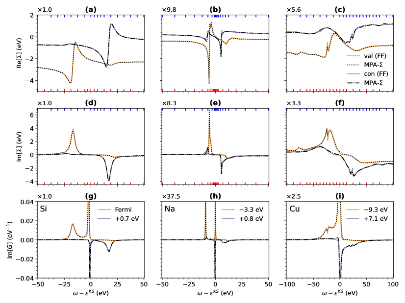
Figure 2: MPA-$\Sigma$ and MPA-$G$ results compared with the corresponding full-frequency (FF) $\Sigma$ and interacting $G$, for semiconducting and metallic materials. The plots show the spectra of a selected valence (yellow) and a conduction (purple) state of Si (left), Na (middle), and Cu (right), with KS energies specified in their respective panels. Panels (a-c) and (d-f) compares the real and imaginary parts of $\Sigma$, and (g-i) the imaginary part of $G$ (g-i), for the respective materials. The solid orange and purple curves indicate the FF results, while the corresponding MPA results are plotted as black dotted (valence) and dashed-dotted (conduction) lines. In the top and center panels, the red (blue) ticks along the horizontal panel borders indicate the distribution of sampling points along the real frequency axis used as input in the MPA-$\Sigma$ interpolation of the given valence (conduction) state.

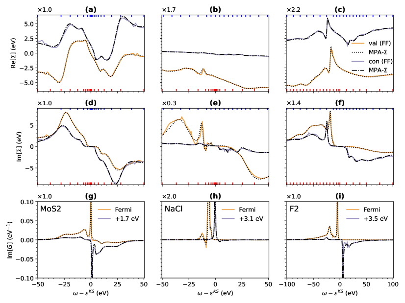
Figure 3: MPA-$\Sigma$ and MPA-$G$ results compared with the corresponding full-frequency (FF) $\Sigma$ and interacting $G$, for materials with reduced dimensionality. The plots show the spectra of a selected valence (yellow) and a conduction (purple) state of the monolayer MoS₂ (left), the NaCl ion-pair (middle) and the F₂ (right) molecule, with KS energies specified in their respective panels. As in Fig. 2, MPA results are plotted as black dotted (valence) and dashed-dotted (conduction) lines, while the red (blue) ticks along the horizontal panel borders indicate the distribution of sampling points along the real frequency axis used as input in the MPA-$\Sigma$ interpolation of the given valence (conduction) state.

III.1 Self-energy and Green’s function of prototypical materials

Fig. 2 shows the real and imaginary parts of the $G_{0}W_{0}$ self-energy, i.e. $\mathrm{Re}~\Sigma$ (a-c) and $\mathrm{Im}~\Sigma$ (d-f), and the imaginary part of the Green’s function, $\mathrm{Im}~G$ (g-i), for a selected valence and a conduction state of Si, Na, and Cu. The solid lines give the results computed with a full-frequency approach (FF), serving as a benchmark, and the (dash-) dotted lines, the MPA-$\Sigma$ approach. The FF approach is evaluated on a grid of 2000 frequency points. For MPA-$\Sigma$, 18 frequencies are used for Si and 22 for Na and Cu, corresponding to $n_{\Sigma}=9$ and $n_{\Sigma}=11$, respectively. The sampling frequencies used in the interpolation are indicated with red (valence) and blue (conduction) ticks along the horizontal panel edges.

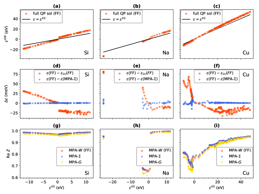
Figure 4: QP energies and renormalization factors of Si (left: a, d, g), Na (middle: b, e, h) and Cu (right: c, f, i) as a function of their DFT-KS energies. Panels (a-c) show the QP solution obtained from the numerical full-frequency (FF) self-energy using a recursive method. Panels (d-f) show the difference between the FF QP equation and the FF linearized results (red squares) and the analytical MPA-$\Sigma$ solution (blue circles). Panels (g-i) correspond to $\mathrm{Re}~Z$ obtained with the FF linearized equation evaluated with Eq. (11) (red squares), the solution of the linearized QP equation within MPA-$\Sigma$ evaluated with Eq. (13) (blue circles), and the spectral weight of the QP pole in the MPA-$G$ representation as defined in Eq. (16) (yellow triangles).

The self-energies of Si and Na have the typical two-pole structure characteristic of systems with a screening potential dominated by a single plasmon pole. As seen in the denominators of Eq. (10), the two $\Sigma$ poles are the result of the plasmon convoluted, respectively, with valence and conduction states. Cu presents a similar picture, but with several plasmon-like poles in $W_{0}$, as can be seen in Ref. [40], that couple with the single-particle poles of $G_{0}$, resulting in a richer structure of $\Sigma^{G_{0}W_{0}}$.

We also tested the MPA-$\Sigma$ description for the MoS₂ monolayer, the NaCl ion-pair, and the F₂ molecule, i.e., materials with lower dimensionality. The results are shown in Fig. 3. We used an MPA-$\Sigma$ representation with 10, 11 and up to 14 poles for MoS₂, NaCl and F₂, respectively. Both Figs. 2 and  3 demonstrate an excellent agreement of MPA-$\Sigma$ and MPA-$G$ with the FF results.

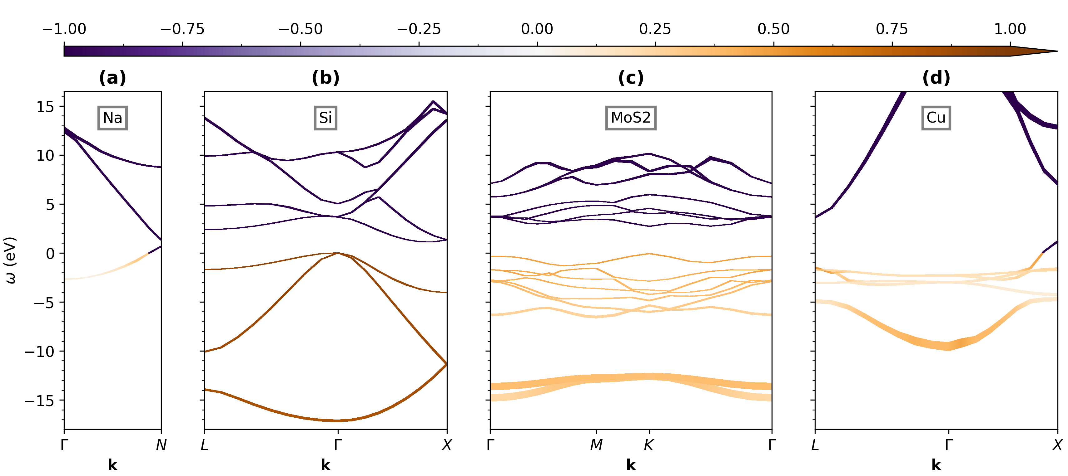
Figure 5: Band structure of Na, Si, monolayer MoS₂ and Cu, with a variable width representing the imaginary part of the quasiparticles $\mathrm{Im}~[\epsilon_{n{\mathbf{k}}}]$. The colormap is given by $-\text{sign}\left(\mathrm{Re}~[\epsilon_{n{\mathbf{k}}}]\right)\mathrm{Re}~[Z_{n{\mathbf{k}}}]$, representing the renormalization factor for valence (orange shades) and conduction (purple shades) states.

In the calculations described above, the $\Sigma$ samplings were adapted to each particular system and states. It is however convenient to apply the same general scheme for the MPA-$\Sigma$ sampling of all the states of each system. To this end, we chose the same type of frequency distribution and number of poles that converge MPA-$W$ for each system. In the case of $\Sigma$, the distribution is centered at each DFT-KS energy, with a small asymmetry on the frequency sampling, i.e., 1 or 2 frequency points more on the negative (positive) side for valence (conduction) states. The total number of frequency points is given by $2n_{\Sigma}$, with $n_{\Sigma}=9$ for Si and Na, and $n_{\Sigma}=11$ for Cu.

Fig. 4 shows the QP energies and $\mathrm{Re}~Z$ of a set of valence and conduction bands of Si, Na, and Cu, in a wide range of energies and momenta. Panels (a-c) show the $G_{0}W_{0}$ energies found by recursively solving the QP equation in Eq. (5) with the FF representation, used here as a reference. They show the expected $GW$ stretching of the KS bands and, for Si, band gap opening. Panels (d-f) compare the difference between the results of the non-linearized FF and the linearized FF QP equation, $\Delta\varepsilon^{\text{lin-FF}}=\varepsilon^{\text{FF}}-\varepsilon^{\text{lin-FF}}$, (red squares), and the difference between the non-linearized FF and the analytical MPA-$\Sigma$ results, $\Delta\varepsilon^{\text{MPA-}\Sigma}=\varepsilon^{\text{FF}}-\varepsilon^{\text{MPA-}\Sigma}$, (blue circles). For valence states $\Delta\varepsilon^{\text{lin-FF}}$ increases with the distance from the Fermi level, consistent with the general trends for materials (see e.g., Ref. [64]). In contrast, $\Delta\varepsilon^{\text{MPA-}\Sigma}$ is almost zero for most of the valence and conduction states, with the exception of a few quasiparticles with more structure in the self-energy around $\omega=0$. This good agreement between MPA-$\Sigma$ and FF demonstrates the accuracy of the MPA-$\Sigma$ method, even with a simple frequency sampling scheme.

As mentioned in Sec. II.3, solving the linearized QP equation requires $\Sigma$ to be computed for one or two frequency points, whereas MPA-$\Sigma$ requires about 20. While the additional sampling points do increase computational costs, this comes with a significant improvement in accuracy. Critically, MPA-$\Sigma$ also allows for a straightforward evaluation of $\Sigma$ in its full-frequency range and gives access to an analytical representation of $G$.

Panels (g-i) of Fig. 4 show the renormalization factor corresponding to the reference FF data evaluated with Eq. (11) (red squares) and the MPA-$\Sigma$ representation of Eq. (13) (blue circles). In both cases, $Z$ is calculated from the local derivative of $\Sigma$, according to Eq. (7). They differ by less than 0.003, 0.010 and 0.025 for all the quasiparticles of Si, Na, and Cu, respectively. The results labeled MPA-$G$ (yellow triangles) were obtained with the definition proposed in Eq. (16), in which $Z$ is given by the largest residue of $G$. For most of the quasiparticles, $Z^{\text{MPA-}\Sigma}$ is quite similar to $Z^{\text{MPA-}G}$; however, for the Na and Cu states with more intense satellites ($\mathrm{Re}~Z\lesssim 0.8$), the deviation can increase to 0.045 and 0.070 respectively, which states that these two $Z$ definitions differ on a fundamental level. A detailed analysis of their differences is presented in Sec. III.3.

Fig. 5 shows the QP band structure of Na (a), Si (b), monolayer MoS₂ (c), and Cu (d). The width of the lines gives the imaginary part of the QP poles $\mathrm{Im}~[\epsilon_{n{\mathbf{k}}}]$, while the color shade indicates the value of the renormalizaion factors $\mathrm{Re}~[Z_{n{\mathbf{k}}}]$ for valence (orange shades) and conduction (purple shades) bands. In general, we find that both $\mathrm{Im}~[\epsilon_{n{\mathbf{k}}}]$ and $\mathrm{Re}~[Z_{n{\mathbf{k}}}]$ increase further away from the Fermi level, as a result of the QP pole and the satellites broadening and merging in a single peak. However, in the energy range in which multiple bands of different character cross, the picture becomes more complex showing a non-monotonic behavior. The metallic band of Na is an exception, with $\mathrm{Im}~[\epsilon_{n{\mathbf{k}}}]$ and $\mathrm{Re}~[Z_{n{\mathbf{k}}}]$ decreasing without crossing any other band. This is in line with the increased weight of the satellites, as discussed in Sec. III.2.

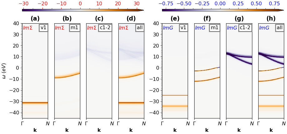
Figure 6: Spectral self-energy (panels (a-d)) and Green’s function (panels (e-h)) band structures of Na, for the first valence state (a, e), the metallic band (b, f), the first two valence bands (c, g) and their combinations (d, h).

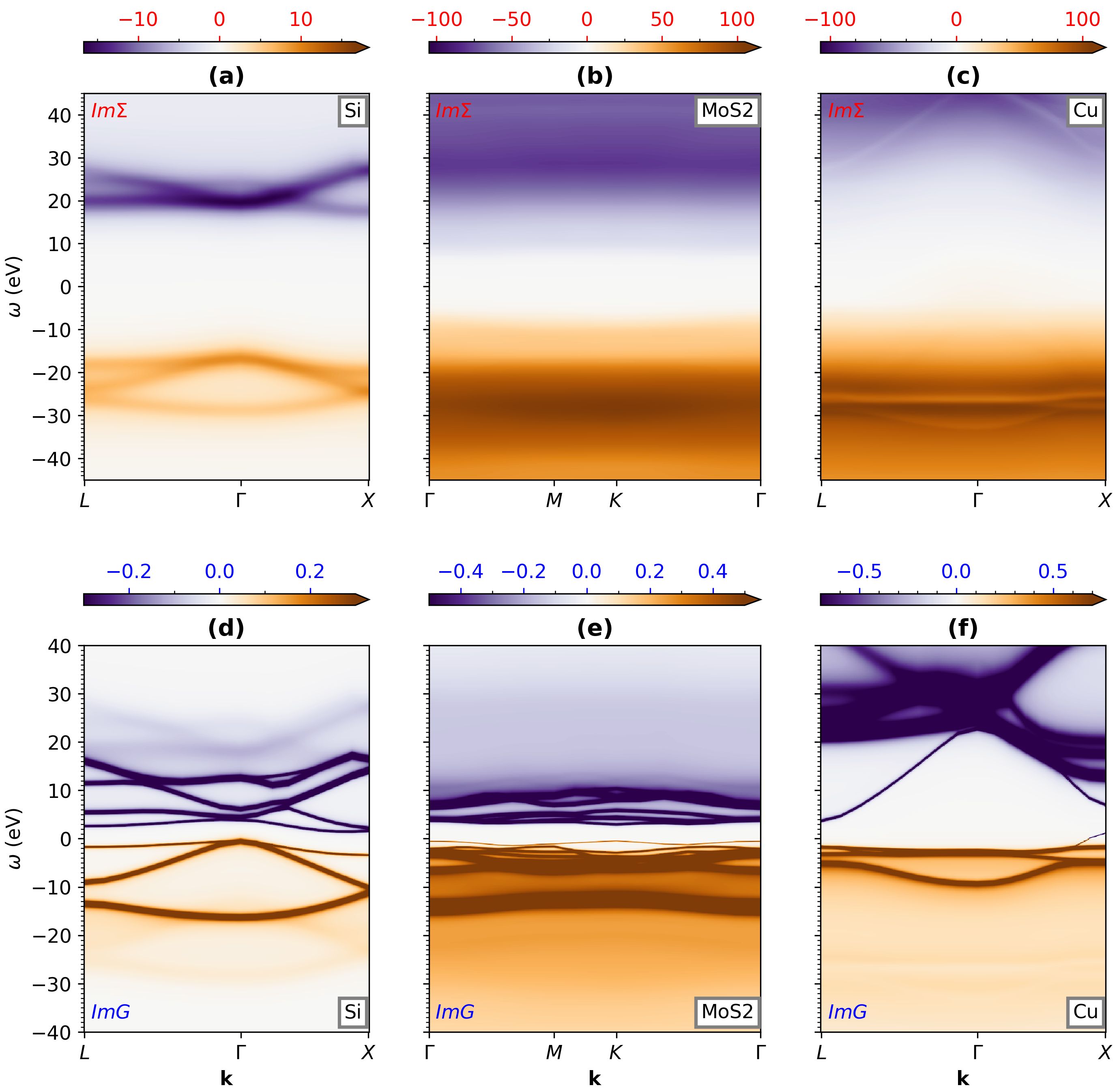
Figure 7: Spectral self-energy (a-c) and Green’s function (d-f) band structure of Si (left panels), MoS₂ (central panels), Cu (right panels). We considered the first 4 valence and 6 conduction bands of Si along the $L\Gamma X$ path, 9 valence and 7 conduction bands of MoS₂ along the $\Gamma MK\Gamma$ path, and 6 valence and 9 conduction bands of Cu along the $L\Gamma X$ path.

III.2 Spectral band structures

The spectral function probed in photoemission and inverse photoemission experiments is the sum of the spectral function of each state, corresponding respectively to valence and conduction bands, according to the polarization of the incoming light [8]. In order to simultaneously represent an uneven number of valence and conduction states, we have defined the following spectral functions of the self-energy and the Green’s function:

$$\mathrm{Im}~\Sigma_{{\mathbf{k}}}(\omega)\equiv\frac{1}{n_{v}}\sum_{v}^{n_{v}}\mathrm{Im}~\Sigma_{v{\mathbf{k}}}(\omega)+\frac{1}{n_{c}}\sum_{c}^{n_{c}}\mathrm{Im}~\Sigma_{c{\mathbf{k}}}(\omega)$$ (17)

$$\mathrm{Im}~G_{{\mathbf{k}}}(\omega)\equiv\frac{1}{n_{v}}\sum_{v}^{n_{v}}\mathrm{Im}~G_{v{\mathbf{k}}}(\omega)+\frac{1}{n_{c}}\sum_{c}^{n_{c}}\mathrm{Im}~G_{c{\mathbf{k}}}(\omega),$$ (18)

where $v$ and $c$ run over valence and conduction states respectively and $n_{v}$ and $n_{c}$ correspond to the total number of valence and conduction bands considered. Since we use time-ordered operators, the spectra have opposite signs for valence and conduction states. We include a normalization based on the number of valence and conduction bands to balance the background intensity of the two regions, and facilitate its visualization. In a detailed comparison with experiment, it would be necessary to properly account for the intensity resulting from the dipole selection rules dictated by the light polarization [8].

Fig. 6 shows $\mathrm{Im}~\Sigma_{{\mathbf{k}}}$ (a-d) and $\mathrm{Im}~G_{{\mathbf{k}}}$ (e-h) of Na along the $\Gamma N$ ${\mathbf{k}}$-path, for the highest non-metallic valence band (v1), for the metallic band that crosses the Fermi level close to $N$ (m1), the two lowest conduction bands (c1-c2), and the combination of all these 4 bands (all). The intensity of the spectra ranges from positive values (orange shades), corresponding to a valence band character, to negative (purple shades), indicating a conduction band character.

$\mathrm{Im}~\Sigma_{{\mathbf{k}}}$ exhibits bands that arise from the coupling of the plasmon with the single KS states, as discussed in the previous section. From now on we will call them $\Sigma$ bands. Essentially, the position of the $\Sigma$ valence (conduction) bands corresponds to the independent-particle bands of $G_{0}$ shifted down (up) by the plasmon energy, $\zeta_{n{\mathbf{k}}}\sim\varepsilon^{\text{KS}}_{n{\mathbf{k}}}\pm\omega_{\text{pl}}$, where $\omega_{\text{pl}}=5.8$ eV [40]. Due to the time ordering, each valence and conduction state has a $\mathrm{Im}~[\Sigma_{n{\mathbf{k}}}](\omega)$ component with the opposite sign discernible, e.g., in panel (b). Therefore, the spectral contribution of each state to the total spectral function $\mathrm{Im}~[\Sigma_{{\mathbf{k}}}]$ is not always trivial, as in the case of the conduction bands in Fig. 6 (d).

$\mathrm{Im}~G_{{\mathbf{k}}}$ (panels (e-h)) also exhibits bands that we will call $G$ bands. There are two types, those coming from the QP pole, $\varepsilon^{\text{QP}}_{n{\mathbf{k}}}$, and those formed from the satellites, $\varepsilon^{\text{sat}}_{n{\mathbf{k}}}$. The QP bands are shifted with respect to the $G_{0}$ bands by the $G_{0}W_{0}$ correction, according to Eq. (5). The satellite bands (called sidebands in Ref. [4]) correspond to replicas of the QP bands located at larger energies. As already seen in Fig. 2 (g-i), the QP peak typically dominates the spectral function. To better discern the satellite structures, we impose a threshold of $|\mathrm{Im}~G_{{\mathbf{k}}}|\leq 0.8$ eV^-1 in the color map. In the case of the metallic band of Na, the intensity of the satellite around the $\Gamma$ point is similar in magnitude to the QP peak, which is interpreted as a plasmaron [75, 4, 76, 5].

Since the satellites emerge from the plasmonic structures in $\Sigma$ [5], the satellite bands are shifted with respect to the QP bands by roughly the energy of the plasmon [19], $\varepsilon^{\text{sat}}_{n{\mathbf{k}}}\sim\varepsilon^{\text{QP}}_{n{\mathbf{k}}}\pm\omega_{\text{pl}}$, and, in turn, are shifted with respect to the $\Sigma$ bands by the $G_{0}W_{0}$ correction, $\varepsilon^{\text{sat}}_{n{\mathbf{k}}}-\zeta_{n{\mathbf{k}}}\sim\varepsilon^{\text{QP}}_{n{\mathbf{k}}}-\varepsilon^{\text{KS}}_{n{\mathbf{k}}}$. The connection between the poles of $\Sigma$ and $G$ is illustrated with the toy model introduced in Sec. III.3. Due to this connection, the accuracy of both the $\Sigma$ and $G$ bands requires a good description of the screening, which can be improved with vertex corrections [75, 19] or cumulant expansions [19, 76, 20, 14]. At finite temperature, electron-phonon interactions are expected to further renormalize and broaden the QP peak [21, 14], as shown for example in Refs. [77, 10, 78] for the case of Cu.

Fig. 7 shows $\mathrm{Im}~\Sigma_{{\mathbf{k}}}$ (top) and $\mathrm{Im}~G_{{\mathbf{k}}}$ (bottom) of the first 4 valence and 6 conduction bands of Si along the $L\Gamma X$ path (a, d), 9 valence and 7 conduction bands of MoS₂ along the $\Gamma MK\Gamma$ path (b, d), and 6 valence and 9 conduction bands of Cu along the $L\Gamma X$ path (c, f). The color maps for the intensity of ${\mathrm{Im}~}G_{{\mathbf{k}}}$ have thresholds of $\pm 0.3$, $\pm 0.5$, and $\pm 0.7$ eV^-1 for Si, MoS₂, and Cu respectively.

Similar to the case of Na, the spectral functions of Si, $\mathrm{Im}~\Sigma_{{\mathbf{k}}}$ (a) and $\mathrm{Im}~G_{{\mathbf{k}}}$ (d), exhibit well defined bands, with $\Sigma$ and satellite bands respectively shifted from the $G_{0}$ and QP bands by the plasmon energy, $\omega_{\text{pl}}=16.6$ eV [39, 19]. This results in a $\Sigma$ band gap given by the KS gap plus twice the plasmon energy ($\varepsilon_{\text{gap}}^{\Sigma}=\varepsilon_{\text{gap}}^{\text{KS}}+2\omega_{\text{pl}}$).

The $\Sigma$ bands of MoS₂ and Cu (Fig. 7 (b) and (c)) are generally broader and overlap more with each other than those of Na and Si. This is in line with both the more complex structure of $\Sigma$ and the fact that the energy separation of the bands is smaller than the width of the main plasmon, located at 10.98 and 26.5 eV for MoS₂ and Cu respectively. As a result, MoS₂ exhibits rather flat and broadened valence and conduction $\Sigma$ bands, with an apparent gap given by secondary peaks at energies smaller than the main plasmon. The valence of Cu also shows a main flat and broadened dispersion, even if some secondary bands are still visible. As a consequence, the satellites of MoS₂ and Cu are also broadened, resulting in the diffused background of Fig. 7 (e, f).

III.3 The quasiparticle picture in MPA models

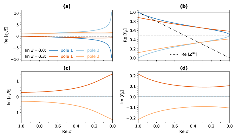
Figure 8: Real and imaginary parts of the scaled poles (a, c) and residues (b, d) of the Green’s function model of Eq. (21) as a function of the $Z$ parameter, where we have fixed $x=0$. The solid horizontal gray line in panel (a) corresponds to $\mathrm{Re}~[\epsilon_{p}/\xi]=1$, while a dashed line is drawn at zero. In panel (b), the gray dashed horizontal line at $\mathrm{Re}~[P_{p}]=0.5$ represents the limit of the QP picture, while the solid line at 1 indicates the sum rule of Eq. (15) ($P_{1}+P_{2}=1$). The dotted black line corresponds to $\mathrm{Re}~[Z^{\text{lin}}]=\mathrm{Re}~Z$, and by contrasting it with $\mathrm{Re}~[Z^{\text{MPA-}G}_{\text{s1}}]=\mathrm{Re}~[P_{1}]$ we are comparing the two definitions of the renormalization factor of Eq. (7) and Eq. (16).

As shown in the previous sections, the self-energy can be approximated by an MPA-$\Sigma$ representation with a small number of poles, from which an MPA-$G$ representation is obtained. Here, we introduce a toy MPA-$\Sigma$ model as a means to analyze the QP picture. We compare the renormalization factor computed from the local derivative of $\Sigma$, as defined in Eq. (7), with the definition in an MPA-$G$ representation proposed in Eq. (16).

We consider a self-energy model with one pole:

$$\Sigma^{\text{s1}}(\omega)=x\xi+\frac{1-Z}{Z}\frac{\xi^{2}}{\omega-\xi},$$ (19)

where $\omega$ is centered on the given QP energy, $x\xi$ accounts for static contributions such as the exchange interaction and vertex corrections, and the second term accounts for correlation with a single pole at the plasmon energy $\xi$. The residue of the pole, $S=\xi^{2}(1-Z)/Z$, is defined in terms of a parameter $Z$ in order to coincide with the local definition of the renormalization factor in Eq. (7), independently of the other two parameters:

$$Z^{\text{lin}}_{\text{s1}}\equiv\left[1-\frac{\partial\Sigma^{\text{s1}}(\omega)}{\partial\omega}\bigg{|}_{\omega=0}\right]^{-1}=Z.$$ (20)

The interacting Green’s function corresponding to Eq. (19) is obtained by inverting the Dyson equation, $G(\omega)=[\omega-\Sigma(\omega)]^{-1}$, resulting in:

$$G^{\text{s1}}(\omega)=\sum_{p=1}^{2}\frac{P^{\text{s1}}_{p}(x,Z)}{\omega-\epsilon^{\text{s1}}_{p}(x,Z,\xi)},$$ (21)

which has 2 poles, $\epsilon^{\text{s1}}_{p}$, with residues $P^{\text{s1}}_{p}$, given by

$$\begin{aligned} \epsilon^{\text{s1}}_{1,2}&=\frac{\xi}{2}\left(1+x\pm\sqrt{D}\right)\\ P^{\text{s1}}_{1,2}&=\frac{1}{2}\left(1\pm\frac{1-x}{\sqrt{D}}\right),\end{aligned}$$ (22)

where

$$D\equiv(1-x)^{2}+4\frac{1-Z}{Z}.$$ (23)

The poles are proportional to $\xi$ and can be rescaled to obtain dimensionless units. The renormalization factor in the MPA-$G$ representation analogous to Eq. (16), corresponds to the largest residue of $G^{\text{s1}}$:

$$Z^{\text{MPA-}G}_{\text{s1}}=\left\{\begin{aligned} &P^{\text{s1}}_{1},\qquad\mathrm{Re}~[P^{\text{s1}}_{1}]\geq\mathrm{Re}~[P^{\text{s1}}_{2}]\\ &P^{\text{s1}}_{2},\qquad\mathrm{Re}~[P^{\text{s1}}_{1}]<\mathrm{Re}~[P^{\text{s1}}_{2}]\end{aligned}\right.$$ (24)

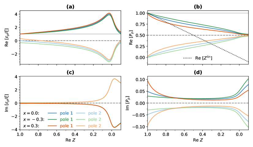
Figure 9: Real and imaginary parts of the scaled poles (a, c) and residues (b, d) of the Green’s function model of Eq. (21) as a function of the $Z$ parameter, where we have fixed its imaginary part to a small value of $\mathrm{Im}~Z=0.01$. The solid and dashed horizontal gray lines and the black dotted line in panel (b) are analogous to Fig. 8.

We first focus on the correlation effects by setting $x=0$. Notice that $Z=1$ corresponds to $S=0$ (zero correlation), while $Z\to 0$ corresponds to the limit of infinite correlation. Fig. 8 shows the real and imaginary parts of the scaled poles, $\epsilon^{\text{s1}}_{p}/\xi$ (panels a, c), and the residues, $P_{p}^{\text{s1}}$ (panels b, d), of $G^{\text{s1}}$ as functions of $\mathrm{Re}~Z$, for $\mathrm{Im}~Z=0$ (blue curves) and $\mathrm{Im}~Z=0.3$ (orange curves). Since $x=0$, $\mathrm{Re}~Z=1$ and $\mathrm{Im}~Z=0$ also correspond to the independent-particle limit, in which the QP state has a zero self-energy correction ($\epsilon^{\text{s1}}_{1}=0$) and carries the whole spectral weight ($P^{\text{s1}}_{1}=Z=1$). As a consequence, the satellite $\epsilon^{\text{s1}}_{2}=\xi$ vanishes ($P^{\text{s1}}_{2}=0$).

In both the cases of $\mathrm{Im}~Z=0$ and $\mathrm{Im}~Z=0.3$, as $\mathrm{Re}~Z$ decreases, $\mathrm{Re}~[\epsilon^{\text{s1}}_{1}]$ goes to negative values with decreasing spectral weight $\mathrm{Re}~[P^{\text{s1}}_{1}]$, while $\mathrm{Re}~[\epsilon^{\text{s1}}_{2}]$ increases from $\xi$ (solid gray line in panel (a)), with increasing $\mathrm{Re}~[P^{\text{s1}}_{2}]$. The finite $\mathrm{Im}~Z$ induces a finite imaginary part in the poles and residues. As $\mathrm{Re}~Z$ decreases, both $\mathrm{Im}~[\epsilon^{\text{s1}}_{p}]$ increase in modulus, while $\mathrm{Im}~[P^{\text{s1}}_{p}]$ decrease despite $\mathrm{Im}~Z$ being constant. The broadening of the poles avoids the infinite correlation limit affecting the curvature of $\mathrm{Re}~[\epsilon^{\text{s1}}_{p}]$ and $\mathrm{Re}~[P^{\text{s1}}_{p}]$ (red vs. blue curves in panels (a, b)).

For all values of $Z$, the first pole has the largest spectral weight and thus $Z^{\text{MPA-}G}_{\text{s1}}=P^{\text{s1}}_{1}$. As illustrated by the dotted black line in panel (b), when we move from the independent-particle limit, the renormalization factor $Z_{\text{s1}}^{\text{lin}}$ starts deviating from $Z_{\text{s1}}^{\text{MPA-}G}$ (dark blue curve), while for $\mathrm{Im}~Z=0.3$ (dark red curve), both definitions already differ at $\mathrm{Re}~Z=1$ and only their real parts coincide around $\mathrm{Re}~[Z]=0.8$. The plot shows that, if $Z$ is taken as an indicator of the validity of the QP picture, the two definitions give inconsistent results, since $\mathrm{Re}~[Z_{\text{s1}}^{\text{MPA-}G}]>0.5$ in the whole interval, even when $\mathrm{Re}~[Z_{\text{s1}}^{\text{lin}}]<0.5$. Therefore, the local definition of the renormalization factor can only be used in the regime of weak correlation ($Z\approx 1$), while in the large correlation limit ($Z\to 0$), the energy position of the poles diverges ($\mathrm{Re}~[\epsilon^{\text{s1}}_{p}]\to\mp\infty$) with similar spectral weight ($\mathrm{Re}~[P^{\text{s1}}_{p}]\to 0.5$).

In Fig. 9 we analyze the effects of the static term. The plots are analogous to Fig. 8. Notice that we have extended the range of the plots to $\mathrm{Re}~Z=-0.1$, to test the QP picture even for extreme values. In this case, we have fixed $\mathrm{Im}~Z=0.01$ and considered three values of $x$, resulting in a picture similar to the one described in Fig. 8, where $\mathrm{Re}~[P^{\text{s1}}_{1}]$ is always larger than $0.5$. The value $x=0$ corresponds to the previously discussed case of a self-energy with only the correlation term. The main effect of a finite value, illustrated with $x=\pm 0.3$, is to change the concavity of the residues according to its sign (panels (b-c)). At variance with $x\leq 0$, for positive values $\mathrm{Re}~[P^{\text{s1}}_{1}]<\mathrm{Re}~Z$ close to $\mathrm{Re}~Z\to 1$, therefore, in this region Eq. (16) produces lower values than the renormalization factor of Eq. (7).

The toy model $\Sigma^{\text{s1}}$ effectively explains the possible causes of the differences between the renormalization factors computed in Fig. 4 with Eqs. (7) and (16). Additional variations in these parameters due to a richer structure of the self-energy are explained by the two-pole self-energy model $\Sigma^{\text{s2}}$ presented in Appendix D. However, if $\Sigma$ is dominated by a single pole the overall picture is the same. Therefore, $\Sigma^{\text{s1}}$ captures the most typical situations when solving the QP equation in prototypical materials. Similar toy MPA models could help clarifying situations in which the QP picture does not hold [4, 64].

IV Conclusions

We have presented MPA-$\Sigma$, a robust method to efficiently approximate the frequency dependence of the $GW$ self-energy as a multipole-Padé representation, typically with around 10 poles. The method is similar to the multipole approximation for the screening interaction, MPA-$W$. Analogous to MPA-$W$, MPA-$\Sigma$ is built from numerical data evaluated on around 20 frequency points in the complex plane, thus avoiding explicit evaluations of the self-energy on dense frequency grids (of the order of 1000 frequencies in our cases). Using MPA-$\Sigma$, it is also possible to solve the QP equation analytically and obtain an MPA-$G$ representation of the interacting Green’s function, from which all the spectral properties can be easily extracted, including the position, broadening, and residue of the QP pole and its satellites.

Combining MPA-$W$ and MPA-$\Sigma$ is a computationally powerful approach, reducing the number of frequency evaluations by a factor $\sim 50^{2}$, compared to full-frequency approaches, while providing spectra with comparable numerical accuracy. The excellent accuracy of the novel method has been verified for several materials: bulk Si, Na and Cu, monolayer MoS₂, the NaCl ion-pair and the F₂ molecule. The efficiency of the MPA method allows us to compute $\Sigma$ and $G$ spectra in a wide energy range. In particular, our results for NaCl and F₂ exhibit features beyond the typical energy range of the $GW$ spectra found in the literature for such molecular species. We have also presented a method for interpolating the spectra of higher-dimensional systems in momentum space, and construct $\Sigma$ and $G$ spectral band structures. For Na, Si, monolayer MoS₂, and Cu, we report full $\Sigma$ and $G$ spectral band structures, while isolating the contributions from the QP pole and the satellites.

The spectral weights of both the QP pole and the satellites computed with MPA-$G$ comply with the sum rule for the number of particles/holes, providing a more general way to define the renormalization factor. Therefore, such analytical representations can be useful in understanding the physical nature of the QP picture and the renormalization factor. We have presented a toy model that captures the most typical situations when solving the QP equation in prototypical materials, exposing the limitations of the renormalization factor as defined from the local derivative of the self-energy, to describe the spectral weight of the most intense peak of the Green’s function beyond the weak correlation regime. Our findings suggest revisiting some literature results on the renormalization factor. They also open the possibility to expand this kind of analysis to the search of materials with exotic spectral properties.

Appendix A MPA-$\Sigma$ interpolation

Consider the exchange and correlation terms of the self-energy, $\Sigma=\Sigma_{\text{x}}+\Sigma_{\text{c}}$; for any state $n{\mathbf{k}}$, the multipole-Padé representation of $\Sigma_{\text{c}}$ can be obtained by solving the following system of $2n_{\Sigma}$ equations and variables:

$$\Sigma_{\text{c}}^{\text{MPA}}(z_{i})\equiv\sum_{p}^{n_{\Sigma}}\frac{S_{p}}{z_{i}-\xi_{p}}=\Sigma_{c}(z_{i})\text{, }i=1,\ldots,2n_{\Sigma}.$$ (25)

Since this model uses an interpolation to reconstruct $\Sigma_{\text{c}}(z)$, the solution will depend on the selected sampling points, $\{z_{i}\}$.

To solve Eq. (25), we follow a similar procedure to the one used for $W_{c}$, by rewriting $\Sigma_{\text{c}}^{\text{MPA}}(z)$ in its Padé form, i.e. as a fraction of two polynomials:

$$\sum_{p}^{n_{\Sigma}}\frac{S_{p}}{z-\xi_{p}}=\frac{A_{n_{\Sigma}-1}(z)}{B_{n_{\Sigma}}(z)},$$ (26)

where the coefficients of the $B_{n_{\Sigma}}(z)$ polynomial can be evaluated from the numerical reference data, $\{z_{i},\Sigma_{c}(z_{i})\}$, using one of the two methods developed in Ref. [39], based on linear algebra and Thiele’s Padé interpolation (see details in section I of Ref. [79]). Moreover, its factorization can be performed using the Companion matrix method [39] and is given by

$$B_{n_{\Sigma}}(z)=\prod_{p}^{n_{\Sigma}}(z-\xi_{p}).$$ (27)

In both methods the sampling points are divided in two sets, which helps to separate the problem of finding the poles, $\xi_{p}$, from the much simpler problem of finding the residues, $S_{p}$, once the poles are known. Such separation is computational advantageous since the nonlinear problem of $2n_{\Sigma}$ variables in Eq. (25), is reduced to two problems of size $n_{\Sigma}$, one nonlinear for the poles and the other linear for the residues. Moreover, by first obtaining the poles, it is then possible to apply physical constrains. We impose to $\xi_{p}=\zeta_{p}+i\varsigma_{p}$ that $\zeta_{p}/\varsigma_{p}<-1$, which guarantees the time ordering and that the poles lay closer to the real frequency axis, as was done for MPA-$W$ [39]. The residues can then be found by solving a simple linear least squares problem (see details in section I of Ref. [79]).

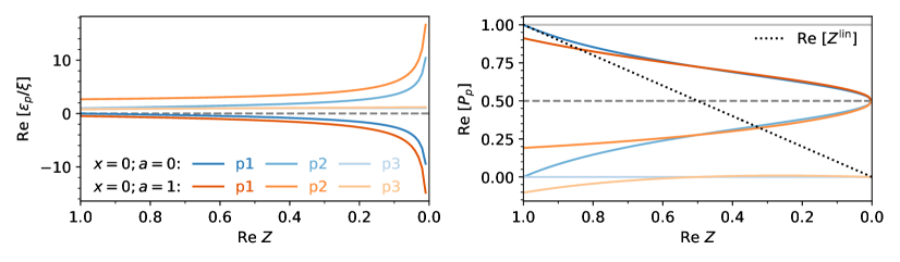
Figure 10: Real part of the poles and residues of the Green’s function model of Eq. (38) as a function of $\mathrm{Re}~Z$, where we have fixed $\mathrm{Im}~Z=0$.

Appendix B MPA-$G$ from MPA-$\Sigma$

Given the MPA-$\Sigma$ representation of the correlation self-energy with $n_{\Sigma}$ poles, the total self-energy can be written in its Padé representation as

$$\Sigma^{\text{MPA}}(z)\equiv\Sigma_{x}+\Sigma_{c}^{\text{MPA}}(z)=\frac{\Sigma_{x}B_{n_{\Sigma}}(z)+A_{n_{\Sigma}-1}(z)}{B_{n_{\Sigma}}(z)}.$$ (28)

Notice that if we apply physical constrains after the factorization in Eq. (27), and fit the residues thereafter, we will need to reconstruct both the $A_{n_{\Sigma}-1}(z)$ and $B_{n_{\Sigma}}(z)$ polynomials from the new poles and residues using Eq. (28), which is straightforward.

We can then compute the interacting Green’s function of Eq. (3) in the MPA approach as

$$G^{\text{MPA}}(z) \equiv\frac{B_{n_{\Sigma}}(z)}{C_{n_{\Sigma}+1}(z)}$$ (29)

$$C_{n_{\Sigma}+1}(z) =zB_{n_{\Sigma}}(z)-\Sigma_{x}B_{n_{\Sigma}}(z)-A_{n_{\Sigma}-1}(z),$$

The poles of $G$ will then correspond to the zeros of $C_{n_{\Sigma}+1}(z)$. Analogous to $B_{n_{\Sigma}}(z)$, the $C_{n_{\Sigma}+1}(z)$ polynomial can be factorized, e.g. using the Companion matrix method [39]:

$$C_{n_{\Sigma}+1}(z)=\prod_{p}^{n_{\Sigma}+1}(z-\epsilon_{p}),$$ (30)

while the residues can be computed using the residue theorem (see also Ref. [57]), as

$$P_{p}=\frac{\prod_{i}^{n_{\Sigma}}(\epsilon_{p}-\xi_{i})}{\prod_{i\neq p}^{n_{\Sigma}+1}(\epsilon_{p}-\epsilon_{i})},$$ (31)

from where it follows that the sum rule of Eq. (15) is satisfied. The resulting multipole-Padé representation of $G$ is then:

$$G^{\text{MPA}}(z)=\sum_{p=1}^{n_{\Sigma}+1}\frac{P_{p}}{z-\epsilon_{p}}.$$ (32)

Appendix C Spline interpolation in ${\mathbf{k}}$-space

To obtain smooth plots of the $\Sigma$ and $G$ spectral band structures, similar to the band structures of the response function computed in Ref. [80], we need to perform an interpolation on ${\mathbf{k}}$ space for each frequency $z_{i}$. Such an interpolation can be cumbersome due to the dispersion of the different bands. The MPA-$\Sigma$ representation can simplify this interpolation since it is sufficient to interpolate the poles and the residues of the multipole-Padé model. The interpolation of the numerical data can be also simplified by considering an auxiliary set of frequencies centered at the KS energies, $z^{\prime}_{i}\equiv z_{i}-\epsilon^{\text{KS}}_{n{\mathbf{k}}}$. Since $z^{\prime}_{i}$ carries the dispersion of the bands, $\Sigma(z^{\prime}_{i},{\mathbf{k}})$ and $G(z^{\prime}_{i},{\mathbf{k}})$ are much smoother than the original $\Sigma(z_{i},{\mathbf{k}})$ and $G(z_{i},{\mathbf{k}})$.

We start by interpolating each KS band $n$:

$$\forall n:\\ {\epsilon^{\text{KS}}_{n}({\mathbf{k}}\text{-grid})}\to f^{\epsilon}_{n}({\mathbf{k}}),$$ (33)

where $f^{\epsilon}_{n}$ is the interpolating function. Similarly, we interpolate $\Sigma$ and $G$ for all frequencies along the direction of each band:

$$\forall n,i: {\Sigma_{n}(z^{\prime}_{i},{\mathbf{k}}\text{-grid})}\to f^{\Sigma}_{n}(z^{\prime}_{i},{\mathbf{k}})$$ (34)

$${G_{n}(z^{\prime}_{i},{\mathbf{k}}\text{-grid})}\to f^{G}_{n}(z^{\prime}_{i},{\mathbf{k}}),$$

where $f^{\Sigma}_{n}$ and $f^{G}_{n}$ are the interpolating function of $\Sigma$ and $G$ respectively. The interpolation for the $\{z_{i}\}$ frequencies can then be obtained as

$$f^{\Sigma/G}_{n}(z_{i},{\mathbf{k}})=f^{\Sigma/G}_{n}[z^{\prime}_{i}+f^{\epsilon}_{n}({\mathbf{k}}),{\mathbf{k}}],$$ (35)

which can be used to evaluate the final spectra on a much denser ${\mathbf{k}}$-grid. We have used first-order splines as the interpolating functions, which is sufficient to obtain smooth spectra for our calculations, although this approach can be applied with other interpolating functions as well.

Appendix D Toy MPA-$\Sigma$ model with two poles

Similar to the $\Sigma^{\text{s1}}$ model discussed in Sec. III.3, here we introduce a toy MPA-$\Sigma$ model with two poles, one at $\epsilon_{1}=\xi$ and the other at a larger energy $\epsilon_{2}=(1+a)\xi$:

$$\Sigma^{\text{s2}}(\omega)=x\xi+\\ \frac{1-2Z}{2Z}\frac{\xi^{2}}{\omega-\xi}+\frac{(1+a)^{2}}{2Z}\frac{\xi^{2}}{\omega+(1+a)\xi}.$$ (36)

where the residues, $S_{1}=\xi^{2}(1-2Z)/(2Z)$ and $S_{2}=\xi^{2}(1+a)^{2}/(2Z)$ are constrained so that the following expression remains invariant, as for $\Sigma^{\text{s1}}$:

$$Z^{\text{lin}}_{\text{s2}}\equiv\left[1-\frac{\partial\Sigma^{\text{s2}}(\omega)}{\partial\omega}\bigg{|}_{\omega=0}\right]^{-1}=Z.$$ (37)

The corresponding MPA-$G$ representation has three poles and a similar form, only with the additional parameter $a$:

$$G^{\text{s2}}(\omega)=\sum_{p=1}^{3}\frac{P^{\text{s2}}_{p}(x,Z,a)}{\omega-\epsilon^{\text{s2}}_{p}(x,Z,a,\xi)}.$$ (38)

Notice that for $a=0$, $\Sigma^{\text{s2}}$ simplifies to $\Sigma^{\text{s1}}$, and therefore this parameter can be used to turn on the second pole. We then fix $x=0$ and $\mathrm{Im}~Z=0$, and compare the two models. Fig. 10 shows the real part of the scaled poles, $\epsilon^{\text{s2}}_{p}/\xi$ (panel (a)), and the residues, $P_{p}^{\text{s2}}$ (panel (b)), of $G^{\text{s2}}$ as functions of $\mathrm{Re}~Z$, for $a=0$ (blue curves) and $a=1$ (orange curves). The overall picture discussed in Sec. III.3 is similar for the two models, with the additional third pole remaining around $\epsilon^{\text{s2}}_{3}=\xi$ with a vanishing residue $P^{\text{s2}}_{3}$. However, a finite $a$ induces a finite $P^{\text{s2}}_{3}$, with its larger modulus at $\mathrm{Re}~Z=1$, which introduces a deviation between $Z^{\text{lin}}_{\text{s2}}$ and $Z^{\text{MPA-}G}_{\text{s2}}=P^{\text{s2}}_{1}$ around $Z=1$.

References

- Aryasetiawan and Gunnarsson [1998] F. Aryasetiawan and O. Gunnarsson, The GW method, Rep. Prog. Phys. 61, 237 (1998).
- Hedin [1999] L. Hedin, On correlation effects in electron spectroscopies and the gw approximation, Journal of Physics: Condensed Matter 11, R489 (1999).
- Onida et al. [2002] G. Onida, L. Reining, and A. Rubio, Electronic excitations: density-functional versus many-body green’s-function approaches, Rev. Mod. Phys. 74, 601 (2002).
- Martin et al. [2016] R. M. Martin, L. Reining, and D. M. Ceperley, Interacting Electrons (Cambridge University Press, Cambridge, 2016).
- Reining [2018] L. Reining, The gw approximation: content, successes and limitations, WIREs Computational Molecular Science 8, e1344 (2018).
- Marzari et al. [2021] N. Marzari, A. Ferretti, and C. Wolverton, Electronic-structure methods for materials design, Nature Materials 20, 736–749 (2021).
- Damascelli [2004] A. Damascelli, Probing the electronic structure of complex systems by arpes, Physica Scripta 2004, 61 (2004).
- Hüfner [2013] S. Hüfner, Photoelectron spectroscopy: principles and applications (Springer Science & Business Media, 2013).
- Dolado et al. [2001] J. S. Dolado, V. M. Silkin, M. A. Cazalilla, A. Rubio, and P. M. Echenique, Lifetimes and mean-free paths of hot electrons in the alkali metals, Phys. Rev. B 64, 195128 (2001).
- Marini et al. [2002a] A. Marini, R. Del Sole, A. Rubio, and G. Onida, Quasiparticle band-structure effects on the d hole lifetimes of copper within the gw approximation, Phys. Rev. B 66, 161104 (2002a).
- Kheifets et al. [2003] A. S. Kheifets, V. A. Sashin, M. Vos, E. Weigold, and F. Aryasetiawan, Spectral properties of quasiparticles in silicon: A test of many-body theory, Phys. Rev. B 68, 233205 (2003).
- Arnaud et al. [2005] B. Arnaud, S. Lebègue, and M. Alouani, Excitonic and quasiparticle lifetime effects on silicon electron energy loss spectra from first principles, Phys. Rev. B 71, 035308 (2005).
- Cazzaniga [2012] M. Cazzaniga, and beyond approaches to quasiparticle properties in metals, Phys. Rev. B 86, 035120 (2012).
- Zhou et al. [2020] J. S. Zhou, L. Reining, A. Nicolaou, A. Bendounan, K. Ruotsalainen, M. Vanzini, J. J. Kas, J. J. Rehr, M. Muntwiler, V. N. Strocov, F. Sirotti, and M. Gatti, Unraveling intrinsic correlation effects with angle-resolved photoemission spectroscopy, Proceedings of the National Academy of Sciences 117, 28596 (2020).
- Hybertsen and Louie [1985] M. S. Hybertsen and S. G. Louie, First-principles theory of quasiparticles: Calculation of band gaps in semiconductors and insulators, Phys. Rev. Lett. 55, 1418 (1985).
- van Schilfgaarde et al. [2006] M. van Schilfgaarde, T. Kotani, and S. Faleev, Quasiparticle self-consistent GW theory, Phys. Rev. Lett. 96, 226402 (2006).
- Hüser et al. [2013] F. Hüser, T. Olsen, and K. S. Thygesen, Quasiparticle gw calculations for solids, molecules, and two-dimensional materials, Phys. Rev. B 87, 235132 (2013).
- Golze et al. [2019] D. Golze, M. Dvorak, and P. Rinke, The GW Compendium: A Practical Guide to Theoretical Photoemission Spectroscopy, Front. Chem. 7, 377 (2019).
- Gumhalter et al. [2016] B. Gumhalter, V. Kovač, F. Caruso, H. Lambert, and F. Giustino, On the combined use of gw approximation and cumulant expansion in the calculations of quasiparticle spectra: The paradigm of si valence bands, Phys. Rev. B 94, 035103 (2016).
- Zhou et al. [2018] J. S. Zhou, M. Gatti, J. J. Kas, J. J. Rehr, and L. Reining, Cumulant green’s function calculations of plasmon satellites in bulk sodium: Influence of screening and the crystal environment, Phys. Rev. B 97, 035137 (2018).
- Nery et al. [2018] J. P. Nery, P. B. Allen, G. Antonius, L. Reining, A. Miglio, and X. Gonze, Quasiparticles and phonon satellites in spectral functions of semiconductors and insulators: Cumulants applied to the full first-principles theory and the fröhlich polaron, Phys. Rev. B 97, 115145 (2018).
- Marini et al. [2002b] A. Marini, G. Onida, and R. D. Sole, Quasiparticle electronic structure of copper in the gw approximation, Phys. Rev. Lett. 88, 016403 (2002b).
- Shishkin and Kresse [2006] M. Shishkin and G. Kresse, Implementation and performance of the frequency-dependent method within the paw framework, Phys. Rev. B 74, 035101 (2006).
- Liu et al. [2015] F. Liu, L. Lin, D. Vigil-Fowler, J. Lischner, A. F. Kemper, S. Sharifzadeh, F. H. da Jornada, J. Deslippe, C. Yang, J. B. Neaton, and S. G. Louie, Numerical integration for ab initio many-electron self energy calculations within the GW approximation, J. Comput. Phys. 286, 1 (2015).
- Godby et al. [1988] R. W. Godby, M. Schlüter, and L. J. Sham, Self-energy operators and exchange-correlation potentials in semiconductors, Phys. Rev. B 37, 10159 (1988).
- F. Aryasetiawan in [2000] F. Aryasetiawan in, Strong coulomb correlations in electronic structure calculations (CRC Press., London, 2000) p. 96, 1st ed., https://doi.org/10.1201/9781482296877.
- Kotani et al. [2007] T. Kotani, M. van Schilfgaarde, and S. V. Faleev, Quasiparticle self-consistent method: A basis for the independent-particle approximation, Phys. Rev. B 76, 165106 (2007).
- Daling et al. [1991] R. Daling, W. van Haeringen, and B. Farid, Plasmon dispersion in silicon obtained by analytic continuation of the random-phase-approximation dielectric matrix, Phys. Rev. B 44, 2952 (1991).
- Engel et al. [1991] G. E. Engel, B. Farid, C. M. M. Nex, and N. H. March, Calculation of the gw self-energy in semiconducting crystals, Phys. Rev. B 44, 13356 (1991).
- Duchemin and Blase [2020] I. Duchemin and X. Blase, Robust Analytic-Continuation Approach to Many-Body GW Calculations, J. Chem. Theory Comput. 16, 1742 (2020).
- Hybertsen and Louie [1986] M. S. Hybertsen and S. G. Louie, Electron correlation in semiconductors and insulators: Band gaps and quasiparticle energies, Phys. Rev. B 34, 5390 (1986).
- Zhang et al. [1989] S. B. Zhang, D. Tománek, M. L. Cohen, S. G. Louie, and M. S. Hybertsen, Evaluation of quasiparticle energies for semiconductors without inversion symmetry, Phys. Rev. B 40, 3162 (1989).
- Godby and Needs [1989] R. W. Godby and R. J. Needs, Metal-insulator transition in kohn-sham theory and quasiparticle theory, Phys. Rev. Lett. 62, 1169 (1989).
- von der Linden and Horsch [1988] W. von der Linden and P. Horsch, Precise quasiparticle energies and hartree-fock bands of semiconductors and insulators, Phys. Rev. B 37, 8351 (1988).
- Engel and Farid [1993] G. E. Engel and B. Farid, Generalized plasmon-pole model and plasmon band structures of crystals, Phys. Rev. B 47, 15931 (1993).
- Farid et al. [1991] B. Farid, G. E. Engel, R. Daling, and W. van Haeringen, Plasmon excitations in crystals, Phys. Rev. B 44, 13349 (1991).
- Lee and Chang [1994] K.-H. Lee and K. J. Chang, First-principles study of the optical properties and the dielectric response of al, Phys. Rev. B 49, 2362 (1994).
- Soininen et al. [2003] J. A. Soininen, J. J. Rehr, and E. L. Shirley, Electron self-energy calculation using a general multi-pole approximation, J. Phys.: Condens. Matter 15, 2573 (2003).
- Leon et al. [2021] D. A. Leon, C. Cardoso, T. Chiarotti, D. Varsano, E. Molinari, and A. Ferretti, Frequency dependence in made simple using a multipole approximation, Phys. Rev. B 104, 115157 (2021).
- Leon et al. [2023] D. A. Leon, A. Ferretti, D. Varsano, E. Molinari, and C. Cardoso, Efficient full frequency gw for metals using a multipole approach for the dielectric screening, Phys. Rev. B 107, 155130 (2023).
- Guandalini et al. [2024] A. Guandalini, D. A. Leon, P. D’Amico, C. Cardoso, A. Ferretti, M. Rontani, and D. Varsano, Efficient GW calculations via interpolation of the screened interaction in momentum and frequency space: The case of graphene, Phys. Rev. B 109, 075120 (2024).
- Raether [1980] H. Raether, Excitation of Plasmons and Interband Transitions by Electrons, 1st ed., Springer Tracts in Modern Physics 88, Vol. 88 (Springer, Berlin, Heidelberg, 1980).
- Giuliani and Vignale [2005] G. Giuliani and G. Vignale, Quantum Theory of the Electron Liquid (Cambridge University Press, 2005).
- Pines [2018] D. Pines, Theory of quantum liquids (CRC Press, 2018).
- Allen and Mikkelsen [1977] J. W. Allen and J. C. Mikkelsen, Optical properties of crsb, mnsb, nisb, and nias, Phys. Rev. B 15, 2952 (1977).
- Smith and Segall [1986] D. Y. Smith and B. Segall, Intraband and interband processes in the infrared spectrum of metallic aluminum, Phys. Rev. B 34, 5191 (1986).
- Lee and Chang [1996] K.-H. Lee and K. J. Chang, Analytic continuation of the dynamic response function using an N-point Padé approximant, Phys. Rev. B 54, R8285 (1996).
- Jin and Chang [1999] Y.-G. Jin and K. J. Chang, Dynamic response function and energy-loss spectrum for Li using an N-point Padé approximant, Phys. Rev. B 59, R8285 (1999).
- Kas et al. [2007] J. J. Kas, A. P. Sorini, M. P. Prange, L. W. Cambell, J. A. Soininen, and J. J. Rehr, Many-pole model of inelastic losses in x-ray absorption spectra, Phys. Rev. B 76, 195116 (2007).
- Kas et al. [2009] J. J. Kas, J. Vinson, N. Trcera, D. Cabaret, E. L. Shirley, and J. J. Rehr, Many-Pole Model of Inelastic Losses Applied to Calculations of XANES, J. Phys. Conf. Ser. 190, 012009 (2009).
- Liang and Yang [2015] Y. Liang and L. Yang, Carrier plasmon induced nonlinear band gap renormalization in two-dimensional semiconductors, Phys. Rev. Lett. 114, 063001 (2015).
- Champagne et al. [2023] A. Champagne, J. B. Haber, S. Pokawanvit, D. Y. Qiu, S. Biswas, H. A. Atwater, F. H. da Jornada, and J. B. Neaton, Quasiparticle and optical properties of carrier-doped monolayer mote2 from first principles, Nano Letters 23, 4274 (2023), pMID: 37159934.
- Lihm and Park [2024] J.-M. Lihm and C.-H. Park, Plasmon-phonon hybridization in doped semiconductors from first principles, Phys. Rev. Lett. 133, 116402 (2024).
- Riegera et al. [1999] M. M. Riegera, L. Steinbeck, I. D. White, H. N. Rojas, and R. W. Godby, The gw space-time method for the self-energy of large systems, Comput. Phys. Commun. 117, 211 (1999).
- Soininen et al. [2005] J. A. Soininen, J. J. Rehr, and E. L. Shirley, Multipole representation of the dielectric matrix, Phys. Scripta 2005, 243 (2005).
- van Setten et al. [2015] M. J. van Setten, F. Caruso, S. Sharifzadeh, X. Ren, M. Scheffler, F. Liu, J. Lischner, L. Lin, J. R. Deslippe, S. G. L. C. Yang, F. Weigend, J. B. Neaton, F. Evers, and P. Rinke, GW100: Benchmarking G0W0 for Molecular Systems, J. Chem. Theory Comput. 11, 5665 (2015).
- Chiarotti et al. [2022] T. Chiarotti, N. Marzari, and A. Ferretti, Unified green’s function approach for spectral and thermodynamic properties from algorithmic inversion of dynamical potentials, Phys. Rev. Res. 4, 013242 (2022).
- Chiarotti et al. [2024] T. Chiarotti, A. Ferretti, and N. Marzari, Energies and spectra of solids from the algorithmic inversion of dynamical hubbard functionals, Phys. Rev. Res. 6, L032023 (2024).
- Ferretti et al. [2024] A. Ferretti, T. Chiarotti, and N. Marzari, Green’s function embedding using sum-over-pole representations, Phys. Rev. B 110, 045149 (2024).
- Ismail-Beigi [2010] S. Ismail-Beigi, Correlation energy functional within the GW-RPA: Exact forms, approximate forms, and challenges, Phys. Rev. B 81, 195126 (2010).
- Guo and Liu [2024] Z. Guo and J. Liu, High- and low-energy many-body effects of graphene in a unified approach, https://arxiv.org/abs/2409.14658v2 (2024).
- Lehmann and Taut [1972] G. Lehmann and M. Taut, On the numerical calculation of the density of states and related properties, Phys. Status Solidi (b) 54, 469 (1972).
- Farid [2002] B. Farid, Dynamical correlation functions expressed in terms of many-particle ground-state wavefunction; the dynamical self-energy operator, Philosophical Magazine B 82, 1413 (2002).
- Rasmussen et al. [2021] A. Rasmussen, T. Deilmann, and K. S. Thygesen, Towards fully automatized GW band structure calculations: What we can learn from 60.000 self-energy evaluations, NPJ Comput. Mater. 7 (2021).
- von Barth and Holm [1996] U. von Barth and B. Holm, Self-consistent results for the electron gas: Fixed screened potential within the random-phase approximation, Phys. Rev. B 54, 8411 (1996).
- Marini et al. [2009] A. Marini, C. Hogan, M. Grüning, and D. Varsano, yambo: An ab initio tool for excited state calculations, Comput. Phys. Commun. 180, 1392 (2009).
- Sangalli et al. [2019] D. Sangalli, A. Ferretti, H. Miranda, C. Attaccalite, I. Marri, E. Cannuccia, P. Melo, M. Marsili, F. Paleari, A. Marrazzo, G. Prandini, P. Bonfà, M. O. Atambo, F. Affinito, M. Palummo, A. Molina-Sánchez, C. Hogan, M. Grüning, D. Varsano, and A. Marini, Many-body perturbation theory calculations using the yambo code, J. Phys.: Condens. Matter 31, 325902 (2019).
- Mortensen et al. [2024] J. J. Mortensen, A. H. Larsen, M. Kuisma, A. V. Ivanov, A. Taghizadeh, A. Peterson, A. Haldar, A. O. Dohn, C. Schäfer, E. Ö. Jónsson, E. D. Hermes, F. A. Nilsson, G. Kastlunger, G. Levi, H. Jónsson, H. Häkkinen, J. Fojt, J. Kangsabanik, J. Sødequist, J. Lehtomäki, J. Heske, J. Enkovaara, K. T. Winther, M. Dulak, M. M. Melander, M. Ovesen, M. Louhivuori, M. Walter, M. Gjerding, O. Lopez-Acevedo, P. Erhart, R. Warmbier, R. Würdemann, S. Kaappa, S. Latini, T. M. Boland, T. Bligaard, T. Skovhus, T. Susi, T. Maxson, T. Rossi, X. Chen, Y. L. A. Schmerwitz, J. Schiøtz, T. Olsen, K. W. Jacobsen, and K. S. Thygesen, GPAW: An open Python package for electronic structure calculations, The Journal of Chemical Physics 160, 092503 (2024).
- Gesenhues et al. [2017] J. Gesenhues, D. Nabok, M. Rohlfing, and C. Draxl, Analytical representation of dynamical quantities in from a matrix resolvent, Phys. Rev. B 96, 245124 (2017).
- Giannozzi et al. [2009] P. Giannozzi, S. Baroni, N. Bonini, M. Calandra, R. Car, C. Cavazzoni, D. Ceresoli, G. L. Chiarotti, M. Cococcioni, I. Dabo, A. D. Corso, S. de Gironcoli, S. Fabris, G. Fratesi, R. Gebauer, U. Gerstmann, C. Gougoussis, A. Kokalj, M. Lazzeri, L. Martin-Samos, N. Marzari, F. Mauri, R. Mazzarello, S. Paolini, A. Pasquarello, L. Paulatto, C. Sbraccia, S. Scandolo, G. Sclauzero, A. P. Seitsonen, A. Smogunov, P. Umari, and R. M. Wentzcovitch, QUANTUM ESPRESSO: a modular and open-source software project for quantum simulations of materials, J. Phys.: Condens. Matter 21, 395502 (2009).
- Giannozzi et al. [2017] P. Giannozzi, O. Andreussi, T. Brumme, O. Bunau, M. B. Nardelli, M. Calandra, R. Car, C. Cavazzoni, D. Ceresoli, M. Cococcioni, N. Colonna, I. Carnimeo, A. D. Corso, S. de Gironcoli, P. Delugas, R. A. DiStasio, A. Ferretti, A. Floris, G. Fratesi, G. Fugallo, R. Gebauer, U. Gerstmann, F. Giustino, T. Gorni, J. Jia, M. Kawamura, H.-Y. Ko, A. Kokalj, E. Küçükbenli, M. Lazzeri, M. Marsili, N. Marzari, F. Mauri, N. L. Nguyen, H.-V. Nguyen, A. O. de-la Roza, L. Paulatto, S. Poncé, D. Rocca, R. Sabatini, B. Santra, M. Schlipf, A. P. Seitsonen, A. Smogunov, I. Timrov, T. Thonhauser, P. Umari, N. Vast, X. Wu, and S. Baroni, Advanced capabilities for materials modelling with Quantum ESPRESSO, J. Phys.: Condens. Matter 29, 465901 (2017).
- Perdew et al. [1996] J. P. Perdew, K. Burke, and M. Ernzerhof, Generalized gradient approximation made simple, Phys. Rev. Lett. 77, 3865 (1996).
- Hamann [2013] D. R. Hamann, Optimized norm-conserving vanderbilt pseudopotentials, Phys. Rev. B 88, 085117 (2013).
- Guandalini et al. [2023] A. Guandalini, P. D’Amico, A. Ferretti, and D. Varsano, Efficient GW calculations in two dimensional materials through a stochastic integration of the screened potential, npj Computational Materials 9, 44 (2023).
- Guzzo et al. [2011] M. Guzzo, G. Lani, F. Sottile, P. Romaniello, M. Gatti, J. J. Kas, J. J. Rehr, M. G. Silly, F. Sirotti, and L. Reining, Valence electron photoemission spectrum of semiconductors: Ab initio description of multiple satellites, Phys. Rev. Lett. 107, 166401 (2011).
- Caruso and Giustino [2016] F. Caruso and F. Giustino, The GW plus cumulant method and plasmonic polarons: application to the homogeneous electron gas*, Eur. Phys. J. B 89, https://doi.org/10.1140/epjb/e2016-70028-4 (2016).
- Gerlach et al. [2001] A. Gerlach, K. Berge, A. Goldmann, I. Campillo, A. Rubio, J. M. Pitarke, and P. M. Echenique, Lifetime of d holes at cu surfaces: Theory and experiment, Phys. Rev. B 64, 085423 (2001).
- Tamai et al. [2013] A. Tamai, W. Meevasana, P. D. C. King, C. W. Nicholson, A. de la Torre, E. Rozbicki, and F. Baumberger, Spin-orbit splitting of the shockley surface state on Cu(111), Phys. Rev. B 87, 075113 (2013).
- [79] See Supplemental Materials for a detailed description.
- Leon et al. [2024] D. A. Leon, C. Elgvin, P. D. Nguyen, O. Prytz, F. S. Hage, and K. Berland, Unraveling many-body effects in ZnO: Combined study using momentum-resolved electron energy-loss spectroscopy and first-principles calculations, Phys. Rev. B 109, 115153 (2024).