Multi-Class Traffic Assignment using Multi-View Heterogeneous Graph Attention Networks
Abstract
Solving traffic assignment problem for large networks is computationally challenging when conventional optimization-based methods are used. In our research, we develop an innovative surrogate model for a traffic assignment when multi-class vehicles are involved. We do so by employing heterogeneous graph neural networks which uses a multiple-view graph attention mechanism tailored to different vehicle classes, along with additional links connecting origin-destination pairs. We also integrate the node-based flow conservation law into the loss function. As a result, our model adheres to flow conservation while delivering highly accurate predictions for link flows and utilization ratios. Through numerical experiments conducted on urban transportation networks, we demonstrate that our model surpasses traditional neural network approaches in convergence speed and predictive accuracy in both user equilibrium and system optimal versions of traffic assignment.
keywords:
multi-class traffic assignment , graph neural network , traffic flow prediction , flow conservation , heterogeneity[inst1]organization=University of Illinois, Urbana-Champaign, Department of Civil and Environmental Engineering,addressline=205 N Mathews Ave, city=Urbana, postcode=61801, state=IL, country=USA
1 Introduction
Traffic assignment is crucial for analyzing transportation networks, as it enhances our understanding of traffic flow dynamics and provides insights into congestion and environmental impacts (Nie et al., 2004). The primary goal of addressing the traffic assignment problem (TAP) is to analyze traffic flow patterns and identify congestion bottlenecks within road networks. This analysis aids urban planners in devising strategic efforts to alleviate traffic congestion (Seliverstov et al., 2017). Beyond network analysis, traffic assignment has significant implications for regional resilience and urban development. Urban planners utilize traffic assignment to assess network robustness during severe events such as hurricanes (Zou and Chen, 2020) and earthquakes (Liu and Meidani, 2023). These assessments help ensure that transportation infrastructure meets the city’s evolving demands and standards.
There are two major principal approaches to resolving traffic assignment issues: user equilibrium (UE) assignment and system optimum (SO) assignment. Each method is grounded in distinct principles and is suited to different contexts. Traditionally, TAP has been addressed through optimization formulations, leading to the development of numerous optimization-based methods (Lee et al., 2003; Zhang et al., 2023). Recently, neural network techniques such as convolutional neural networks (CNNs) (Fan et al., 2023) and graph neural networks (GNNs) (Rahman and Hasan, 2023) have increasingly been applied to tackle these problems. Particularly when dealing with incomplete origin-destination (OD) demand data, GNNs often outperform optimization-based methods in terms of speed and accuracy, with encoder-decoder models demonstrating superior performance (Liu and Meidani, 2024).
For instance, although scenarios with reduced link capacity are considered, situations where roads are completely closed due to regulatory orders, resulting in different network topology, are often overlooked. Moreover, previous studies typically assume the presence of only a single vehicle class within the network, which does not accurately reflect real-world conditions. In practice, various vehicle classes exist, each with different levels of road accessibility. For example, sedans and small vehicles can navigate most highways, primary, and secondary roads, whereas trucks and other heavy-duty vehicles are generally confined to highways and primary roads, often subject to time-based restrictions. These critical factors have not been accounted for in previous research, thereby limiting the practical applicability and feasibility of the existing methods. These gaps highlight the need for further research to enhance the adaptability and real-world relevance of neural networks in traffic management.
From the perspective of graph neural network formulation, the traffic flow patterns belonging to each vehicle class can be conceptualized as a distinct “view" within the transportation network. That is, each class of vehicle is related to its unique OD demands and available routing options, leading to distinct traffic patterns. This is while the route choice of vehicles of a certain class does in fact influence the routes of other classes, creating interdependencies across these views. As a result, these different views, representing various vehicle classes, interact at the link level in the GNN, causing the interdependent views to shape the overall traffic flow pattern at a system-wide scale. Therefore, it is crucial to enable exchange of information (i.e. message passing) between different views within a GNN model for a multi-class vehicle traffic assignment. To the best of our knowledge, the proposed approach in this paper is the first work addressing this research gap.
To model the interdependencies between the classes, we build upon the model we proposed in (Liu and Meidani, 2024), which was a heterogeneous GNN consisting of physical roads and virtual "Origin-destination" links. We then introduce a novel multi-view heterogeneous graph attention network. Our approach uniquely assigns a distinct GNN view to each vehicle class, with each view utilizing specific features. This enhancement incorporates OD demand data from various vehicle classes, enabling more effective feature propagation across the network. Moreover, we propose a multi-view graph encoder-decoder structure that can be integrated with any existing GNN to calculate the solution of a traffic assignment problem. The encoder-decoder architecture is designed to capture interactions among different vehicle classes, facilitating the estimation of both link flows and link utilization ratios. Additionally, we incorporate a conservation-based loss function that promotes the flow predictions to align with established traffic flow principles. In summary, the key contributions of our study are threefold:
-
1.
This is the first multi-view GNN framework that can handle multi-class vehicle traffic assignment, effectively capturing the complex interdependencies between various vehicle classes and origin-destination demand.
-
2.
The model leverages the conservation of traffic flow principle to enhance the accuracy of flow predictions.
-
3.
The proposed framework is demonstrably capable to predict traffic flows under extreme conditions, such as road closures, restrictions, and altered network topologies that specific to each vehicle classes, thereby broadening its utility in real-world transportation problems.
In this work we demonstrate the efficacy and generalizability of the proposed model through extensive experiments on various road network topologies, link properties, and OD demands. The remainder of this article is structured as follows. Section 2 provides a review of related literature. General backgrounds on the traffic assignment problem, and the graph neural network are presented in Section 3. Section 4 includes the introduction of the proposed multi-view heterogeneous graph attention network for multi-class vehicle traffic assignment. Furthermore, the experiments with urban road networks are presented to demonstrate the accuracy and generalization capability of the proposed framework in Section 5. Finally, the conclusion and discussion of the proposed framework are presented in Section 6.
2 Related Literature
Solving the traffic assignment problem (TAP) has been the focus of many studies. For example, Lee et al. (2003) aimed to improve both convergence and computational efficiency in solving TAP for large-scale traffic networks by proposing a conjugate gradient projection method to enhance traditional gradient projection techniques. Similarly, Babazadeh et al. (2020) introduced a reduced gradient algorithm that selects non-basic paths to effectively manage computational complexity. In the context of multi-class vehicle traffic assignment, Sun and Szeto (2021) proposed a logit-based multi-class ridesharing user equilibrium framework, formulated as a mixed complementarity problem. Their findings demonstrate that policies such as car restrictions, cordon tolling, and subsidization are significantly influenced by the relative performance of transit systems and users’ preferences for driving. Additionally, Xu et al. (2024) addressed the range-constrained traffic assignment problem by considering heterogeneous range anxiety among electric vehicle drivers, showing that heightened anxiety can lead to severe congestion on critical network links.
Recently, neural networks have been successfully used in data reconstruction and generalization (Zhang et al., 2018), making them a promising solution for solving TAPs while addressing the issue of missing origin-destination (OD) demands. However, the application of neural networks in TAPs remains relatively underexplored. A prominent neural network approach in this domain is the use of convolutional neural networks (CNNs), where the transportation network is modeled as a grid map on which the incomplete OD demand is handled, as done in Fan et al. (2023). Another choice for the neural network architecture is the graph neural network (GNN). GNNs solve TAPs by capturing spatial information using graph topology information (Liu and Meidani, 2024a). For instance, Rahman and Hasan (2023) applied graph convolutional neural network to learn traffic flow patterns directly from OD demand and link flow data, offering a scalable solution for large-scale TAPs. Building upon this work, (Liu and Meidani, 2024) and Liu and Meidani (2024b) extended the homogeneous GNN into a heterogeneous GNN that utilizes two different types of links, namely roadway and OD links, to estimate traffic flows in both static and dynamic traffic assignments. However, these approaches have primarily focused on single-class vehicle traffic assignment, and the interactions and interdependencies between different classes of vehicles are not considered. Furthermore, most of the existing neural network approaches focus on in-distribution data prediction, and the traffic flow prediction under unseen scenarios or out-of-distribution data is not fully investigated.
In summary, despite significant advances enabled by neural networks, a fast solution approach for multi-class vehicle traffic assignment and link-wise flow estimation is needed for enhanced traffic management for such problems. Specifically, there is a need to address the interaction between different vehicle classes and to understand how multiple classes of vehicle collectively influence the network flow distribution.
3 Technical Background
3.1 Multi-Class Vehicle Traffic Assignment Problem
The traffic assignment problem involves estimating traffic volumes or flows on each edge in the network, given a graph topology and OD demand values. Specifically, let us consider a transportation network represented as a graph , where denotes the set of vertices (or nodes), which are the intersections of roads, and denotes the edges or roadways connecting the nodes. Furthermore, consider to be the set of vehicle classes. The general form of multi-class vehicle traffic assignment problem can then be formulated as an optimization optimization problem given by
| (1) |
where the flow for vehicle class on link , and is the cost function for link . The link cost function, which is a function of link flow, can represent the travel time, travel distance, or other relevant factors. Additionally, the traffic assignment problem can have different formulations depending on the specific objectives and assumptions. For instance, a multi-class vehicle user equilibrium traffic assignment problem, adapted from (Beckmann et al., 1956), can be formulated as follows:
| (2) | ||||
where the objective function is the summation over all road segments of the integral of the link travel time function between 0 and the link flow, is the link travel time function, is the total demand from source to destination for vehicle class , represents the flow of vehicle class on path from to s. is the binary variable which equals 1 when link is on path to connect and for vehicle class . It is noted that the objective function in Beckmann’s formulation serves more as a mathematical construct for optimization than a direct physical representation.
3.2 Graph Neural Network
In the early architecture of fully connected neural networks applied to scientific problems, the input data structures are normally of a fixed shape, and the predominant applications processed Euclidean data Liu et al. (2020). However, a non-Euclidean data structure such as graph-structured data is pervasive in engineering applications. The complexity and variability of the graph structure data make it inefficient to be processed with conventional neural network architectures. To address this challenge, GNNs are specifically designed to handle graph-structured data. GNNs operate on the node features and edge features and learn to extract embeddings from nodes and edges, aiming to capture the underlying patterns affecting the graph data.
GNNs consist of two major components. The first component is the graph topology, typically represented as a graph , where and represent the node and edge set, respectively. The second component is the feature embedding, including initial node embedding for and initial edge embedding for in lower dimensional space, where and is the dimension of the feature embedding.
GNNs typically involve an update rule at the node level. This update rule in turn involves an aggregation of information from neighboring nodes. There are various neighborhood aggregation approaches that can be effectively used in large-scale graphs. A prominent method is GraphSAGE (Hamilton et al., 2017), which diverges from spectral techniques by performing convolutions directly in the spatial domain. GraphSAGE operates by sampling a fixed-size neighborhood of nodes and aggregating their features to update the target node’s representation. The update rule in GraphSAGE is defined by:
| (3) |
where is the node embedding of node at the layer, denotes the neighborhood of node , is a differentiable function such as mean, sum, or max pooling, is a non-linear activation function, and denotes concatenation. The learnable parameters are represented by at each layer . This aggregation-based method allows for learning node embeddings that incorporate both local graph structure and node feature information, enabling the application of GraphSAGE to inductive learning tasks on graphs that exhibit unseen nodes during training.
As a different approach to modeling graph data, the graph attention network (GAT) offers an innovative method by determining attention weights for each node, which are influenced by its own features and those of its adjacent nodes (Veličković et al., 2017). In this approach, the updated representation of each node at the layer, is computed using
| (4) |
where is a learnable weight matrix, is the attention weight assigned to the node related to its neighboring node , and is an activation function. The attention weights are computed as follows:
| (5) |
where is a learnable vector of weights. By employing a multilayered attention mechanism, the network is capable of capturing progressively intricate graph representations. This adaptive focus on various nodes within their localities enhances the efficacy of the model.
The aforementioned formulation is valid for homogeneous graphs, where all nodes and edges have the same semantic meaning. However, it is noted that real-world graphs are not always homogeneous. For instance, in the literature citation graph, nodes can represent various entities such as papers, authors, and journals, while edges may denote different semantic relationships. When the graph contains different classes of nodes or edges, it is considered as a heterogeneous graph. Utilizing GNNs on heterogeneous graphs offers notable advantages over homogeneous counterparts, particularly in the ability to learn type-specific representations for each node and edge type (Wang et al., 2019; Fu et al., 2020).
| (6) |
where represents the set of edge classes, for instance, the set of vehicle classes. is a class-specific learnable weight matrix for the relation class , and is the attention weight assigned to node considering its relationship class with node . The attention weights for each class are computed as:
| (7) |
where is a relation-specific learnable weight vector, is the set of neighboring nodes connected by relation class to node . HGNNs allow for the aggregation of features across multiple classes of relationships, each contributing differently to the node embeddings. This mechanism facilitates learning more intricate and nuanced representations, enhancing the model’s performance across diverse graph-based tasks. In the following sections, we will leverage the expressiveness of the heterogeneous graph neural network to estimate the traffic flow performance of multiple classes of vehicles.
4 Multi-View Heterogeneous Graph Attention Network for Traffic Assignment
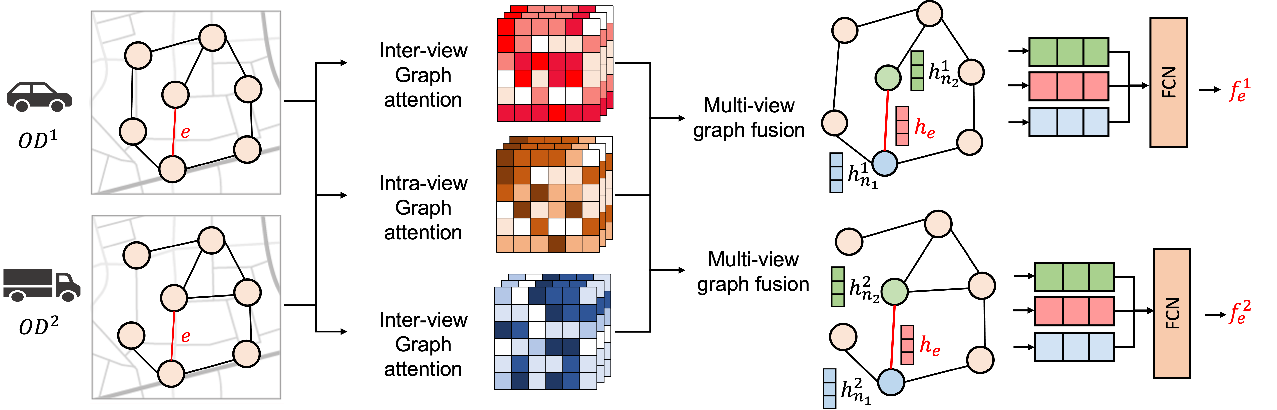
In this section, we introduce the proposed architecture of the multi-view heterogeneous graph attention network (referred to heartoafter as M-HetGAT) for traffic assignment. A schematic of the proposed model is shown in Fig. 1. Each view in the proposed graph neural network represents the traffic flow pattern belonging to one vehicle class. In the following, detailed explanation of each module including feature preprocessing, multi-view graph attention, and multi-view graph fusion are provided.
4.1 Graph Construction & Feature Preprocessing
The heterogeneous graph for multi-class vehicle traffic assignment modeling, denoted as , utilizes a multi-view representation of the transportation network. This multi-view GNN representation is motivated and extended from the single-view GNN model from Liu and Meidani (2024). Additionally, compared with Liu and Meidani (2024), we consider additional interaction between different classes of vehicle. Each view in the proposed graph neural network represents the traffic flow pattern of that particular vehicle class . The view corresponding to vehicle class consists of three distinct components: (1) nodes , which correspond to intersections of roadways; (2) real edges , which represent physical connections between intersections, such as streets or highways; and (3) virtual edges , which are auxiliary links between the origin and destination nodes. The virtual edges between the origin and destination node pairs could compress the number of steps of message-passing for long-range node pairs and discover dependencies between link flows and OD demand. It should be noted that for different views of the graph, the set of real or virtual links may differ. This is because certain classes of vehicles may not have access to certain roadways. Furthermore, the incorporation of virtual links is applied to facilitate enhanced feature updating as an edge augmentation technique.
In the proposed model, the node feature attribute is denoted as , where represents the node set of the view of the graph. Specifically, each row within this matrix corresponds to the feature vector of a single node , including the origin-destination demand for vehicle class as well as geographical coordinates. represents for edge feature of edge belonging to vehicle class . Each row in this matrix includes the free-flow travel time and the link capacity for a single link.
However, in many cases, the raw node attributes exhibit sparsity and lack normalization. To resolve these issues, a preprocessing step is implemented to transform the raw attributes into a more compact initial node embedding in lower-dimensional space through a fully connected network, which represents the updated node embedding of node for vehicle class . This encoding not only preserves the fundamental characteristics of the data but also maintains its semantic integrity. Additionally, we ensure that the edge features are normalized to stabilize their contribution during the subsequent message-passing phases.
4.2 Multi-View Heterogeneous Graph Attention Network
As discussed in Section 3.2, a significant challenge within heterogeneous graphs is the effective propagation of node and edge embeddings, specifically between features from different views. To address this challenge, our model involves a novel multi-view graph attention network that facilitates feature extraction and propagation. This network distinguishes between two types of dependencies critical to multi-class vehicle traffic assignment: intra-class and inter-class dependencies. We utilize a graph transformer-based attention mechanism to enhance feature modeling for intra-class dependencies, focusing on the interactions within the same group of node embeddings. On the other hand, for inter-class dependencies, we explore the interactions among different groups of node embeddings, which is especially critical given the complex interactions modeled in multi-class systems.
To address intra-class dependencies, we build an intra-view graph attention layer for each vehicle class. This involves transforming node features into matrices representing keys, queries, and values to compute attention scores among node pairs. The mathematical formulation for vehicle class can be expressed as:
| (8) |
where is the feature embedding of node at the layer. , , and is the query, key, and value vector at head in encoder where denotes the dimensionality of the feature vectors. are the learnable parameters. We then compute the attention scores among nodes and update the node embedding. Specifically, we first update the node embedding through the virtual link set, then the real link set. Additionally, we incorporate a learnable adaptive weight in computing these scores. This addition of edge-dependent adaptive weights stems from the motivation that variations in low-dimensional node embeddings reflect the variability in node OD demand. In particular, OD pairs are assigned higher attention scores due to their higher influence on traffic flow distribution. By implementing adaptive weights at the edge level, our graph attention model allows for the node feature propagation with the most relevant information via edges, which enhances the model’s contextual comprehension. Mathematically it could be described as follows
| (9) | |||||
where and represent the learnable adaptive weight. represents the un-normalized attention score of the edge at head of the layer; represents the intra-class normalized node embedding of node and represents all the outgoing nodes connected to .
Furthermore, to model interdependencies between different classes, we propose an inter-view graph attention layer. The structure of the inter-view graph attention layer employed in the model is analogous to Equation 8; However, it utilizes a distinct node embedding as the input. Specifically, we concatenate node embeddings from various vehicle classes to generate new inter-class key, query, and value vectors:
| (10) |
These two distinguished node embeddings are crucial for accurately evaluating and forecasting the interactions among different vehicle classes within a network. Similarly, we can calculate the inter-class node embedding using Equation 9 by using the inter-class key, query, and value matrix. Additionally, a residual connection supplements the final output of the layer, ensuring the integration of original input features with learned representations for enhanced model performance. Subsequently, value vectors, normalized by the attention scores, pass through a position-wise feed-forward network (denoted by ), which includes layer normalization (denoted by ). Finally, the output of the multi-view graph attention network is obtained by concatenating the inter-view and intra-view node embeddings from all attention heads, according to
| (11) | |||||
where represents the number of attention heads of the graph attention layer. To enhance the propagation of node features throughout the network, we sequentially stack multiple layers of the graph attention layer. The final output of this stacked graph attention network, denoted as , serves as the input for the subsequent edge-level link flow prediction.
4.3 Graph Edge Prediction
To predict the traffic flow at the edge level, the node embedding of the source node and destination node, and the normalized real edge feature are concatenated and passed through a feed-forward neural network. In this paper, we predict the flow-capacity ratio, denoted by , which is the link flow normalized by the link capacity, according to
| (12) |
where and represent the node embeddings, is the edge features for the real edge belonging to vehicle class , and are the learnable parameters of the feed forward network. The predicted link flows, , for vehicle class can be calculated by multiplying the link capacity with the predicted flow-capacity ratio. Subsequently, selecting an appropriate loss function becomes crucial to ensure the model’s effective convergence. The proposed model employs a composite loss function comprising two components. The first part is the supervised loss which measures the difference between prediction and ground truth values. It consists of two parts: (1) the discrepancy in the flow-capacity ratios, captured by , and (2) the difference in the link flows, captured by . Thus, we will have
| (13) |
where the and represent the ground truth and prediction of flow-capacity ratio on link for vehicle class . The and represent the ground truth and prediction of link flow on link for vehicle class . The second part of the loss function originates from the principle of node-based flow conservation, where the total flow of traffic entering a node equals the total flow of traffic exiting that node. The node-based flow conservation law can be represented mathematically by
| (14) |
where denotes the flow on the link , represents the difference between flow receiving and sending at node , represents the number of OD demand from to . denote the origin-destination node set. The node-based flow conservation law can be added as a regularization term in the total loss function, thereby promoting compliance with flow conservation. In order to incorporate the conservation law into the loss function, we form a conservation loss function given by
| (15) |
where and represent the incoming and outgoing edges for node , respectively. Consequently. the total loss for the flow prediction is the weighted summation of the supervised loss and the conservation loss:
| (16) |
where the , and represent the normalized weights for the flow-capacity ratio supervised loss, link flow supervised loss, and the conservation loss, respectively.
5 Numerical Experiments
In this work, we consider two numerical experiments to evaluate the accuracy, efficiency, and generalization capability of our proposed GNN model. The first experiment focuses on urban transportation networks under normal conditions, while the second experiment models these networks under scenarios involving partial road closures.
5.1 Experiments on Urban Transportation Networks
5.1.1 Characteristics of networks
This paper examines three urban transportation networks as case studies: the Sioux Falls network, East Massachusetts Network (EMA), and Anaheim network (see Table 1 for their network information). Detailed information regarding the topology of these networks, characteristics of their links, and the OD demand was obtained from (Bar-Gera et al., 2023). In this problem, two vehicle classes are considered: cars and trucks.
| Network Name | Average degree | Aggregated OD Demand | ||
| Sioux Falls | 24 | 76 | 3.17 | 316,290 |
| EMA | 74 | 258 | 3.49 | 226,168 |
| Anaheim | 416 | 914 | 3.05 | 311,270 |
Furthermore, in order to reflect the larger space occupancy of trucks and their impact on traffic flow, we adopt a passenger car equivalent ratio equal to 1.9, which considers both the heavy-duty and light-duty trucks Pulugurtha and Jain (2022). To create variations from the perspective of both demand and the link capacity, we scaled the demand by a scaling factor according to
| (17) |
where is the default OD demand between source and destination and is the uniformly distributed random scaling factor for the OD pair (, ). Additionally, to account for variations in network properties, variable link capacities are created according to
| (18) |
where is the original link capacity for link , and is the scaling factor for link . Capacity variations are considered to be due to traffic accidents, road construction/damage, and adverse weather conditions, which reduce the link capacity. In this work, the level of capacity reduction is randomly drawn from a uniform distribution between 0.8 and 1, i.e., .
5.1.2 Experiment setup
The dataset of each network includes 5,000 entries. These entries are divided into training and testing subsets by 80% and 20% of the dataset. To ensure the robustness of the model, it is critical to confirm that the distribution of datasets reflects realistic variations in network conditions and demand patterns. The lowest observed coefficient of variation for link capacity and OD demand across the networks is 0.45 and 0.22, respectively. This variation suggests that the datasets are adequately diverse, enabling the exploration of different scenarios.
The training and testing datasets were generated using the Frank-Wolfe algorithm to solve User Equilibrium Traffic Assignment Problems (UE-TAP) and System Optimal Traffic Assignment Problems (SO-TAP) (Fukushima, 1984). Convergence of the algorithm is achieved when the square root of the sum of squared differences in link flows between two consecutive iterations, normalized by the total link flow, is below a threshold of 1e-5. The GNN model is developed in PyTorch (Paszke et al., 2019) and the Deep Graph Library (DGL) (Wang et al., 2019), featuring a preprocessing layer that includes a three-layer fully connected neural network with an embedding dimension of 32. The model architecture consists of four multi-view graph attention layers. The number of heads in the attention mechanism is 8. Hyperparameters were carefully selected, setting the hidden layer size at 64, which is common in neural network configuration (Liu and Meidani, 2023). Training parameters were set with a learning rate of 0.001 and a batch size of 128. The loss function weights, corresponding to , , and in equation 16, were set at 1.0, 0.005, and 0.05, respectively, to balance the model’s training emphasis on different error components.
We conducted a performance evaluation of our proposed multi-view heterogeneous graph attention model (referred to by M-HetGAT), and compared it against three alternative models incorporating multi-view architectures: the multi-view graph attention network (M-GAT), the multi-view graph convolution network (M-GCN), and the multi-view inductive graph representation learning model (M-GraphSAGE). The M-GAT, M-GCN, and M-graphSAGE implementations consist of four layers of graph message passing followed by three fully connected layers, each with an embedding size of 64. We assessed model performance using two key metrics, including mean absolute error (MAE) and root mean square error (RMSE):
| (19) |
| (20) |
where and respectively represent the ground truth and predicted values for quantity of interest. We conducted a 5-fold cross-validation for each experiment to ensure the robustness of our results across different subsets of the data.
5.1.3 Numerical results
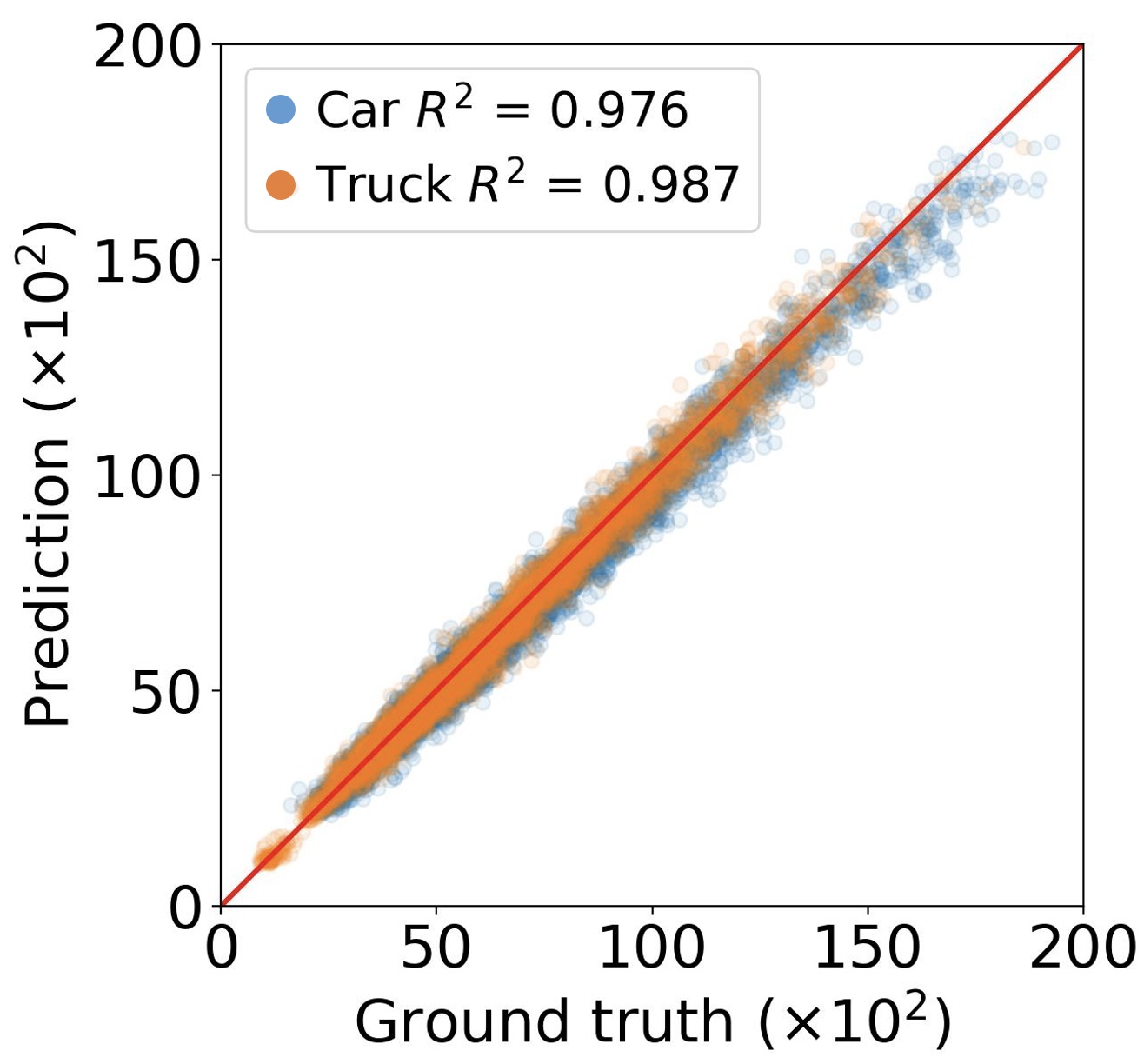
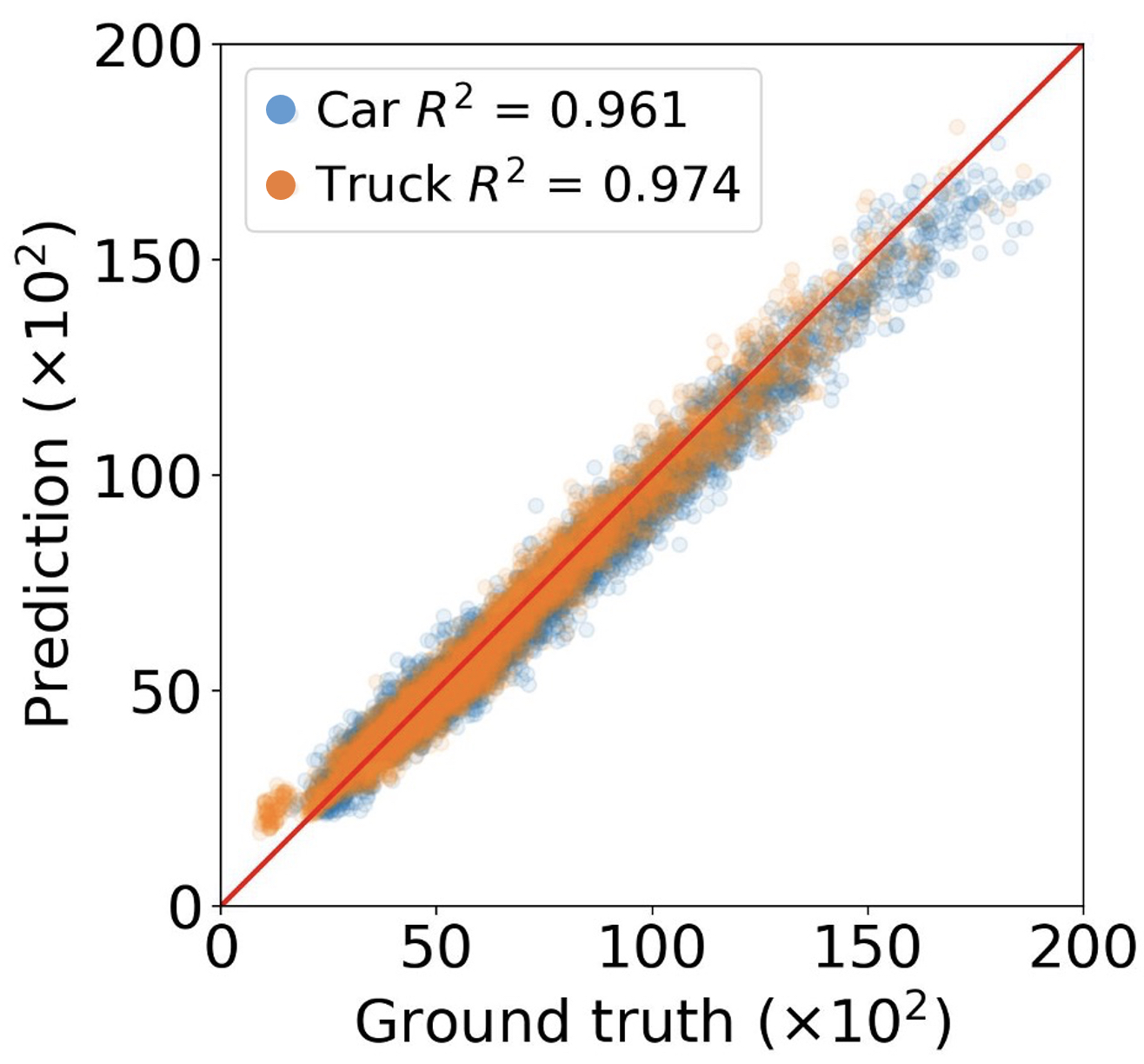
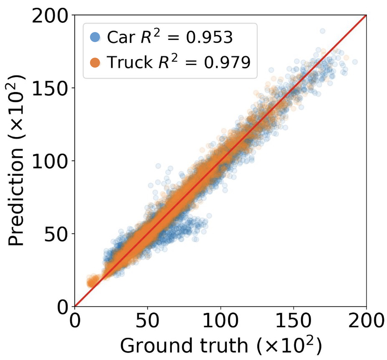
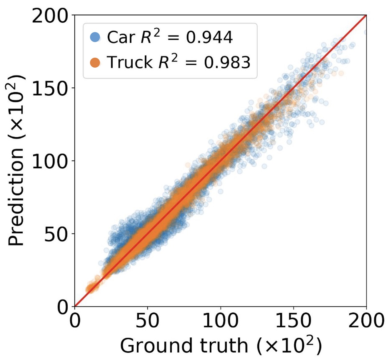
The experiments under the urban road network are conducted in two different settings: the system optimal (SO-TAP) and user equilibrium (UE-TAP) traffic assignment problems. Figure 2 illustrates the correlation between the predicted and actual link flows in the Sioux Falls network for both cars and trucks. The analysis involves predicting the flow-capacity ratios for 10,000 edges using various models: M-HetGAT, M-GAT, M-GCN, and M-graphSAGE. The correlation coefficients, exceeding 0.94 as depicted in Figure 2, underscore the effectiveness of the multi-view graph attention mechanisms in accurately forecasting link flows and utilization across different vehicle classes. To illustrate, The inter-view message passing helps the GNN model to understand the interaction between different vehicle classes. On the other hand, the intra-view message passing would help the single-view GNN model to predict the traffic flow for each class of vehicles accurately. Moreover, the results reveal that the heterogeneous graph attention model, M-HetGAT, consistently surpasses the performance of other models such as M-GAT, M-GCN, and M-graphSAGE in pairwise comparisons, demonstrating its superior capability in handling multi-class vehicle flow predictions on urban road networks.
| Setting | Metric | Model | Sioux Falls | EMA | Anaheim | |||||||||||||
| Car | Truck | Car | Truck | Car | Truck | |||||||||||||
| MAE | RMSE | MAE | RMSE | MAE | RMSE | MAE | RMSE | MAE | RMSE | MAE | RMSE | |||||||
|
|
M-GAT | 4.71 | 5.99 | 3.86 | 5.05 | 0.70 | 1.10 | 0.68 | 1.08 | 3.27 | 4.82 | 0.82 | 1.22 | ||||
| M-GCN | 6.52 | 10.24 | 3.46 | 4.98 | 0.62 | 1.05 | 0.64 | 1.11 | 4.91 | 6.95 | 0.69 | 0.99 | ||||||
| M-GraphSAGE | 4.33 | 5.59 | 2.78 | 3.71 | 0.48 | 0.77 | 0.41 | 0.64 | 3.22 | 4.76 | 0.75 | 1.09 | ||||||
| M-HetGAT | 2.85 | 3.71 | 2.11 | 2.81 | 0.28 | 0.45 | 0.25 | 0.40 | 3.17 | 4.24 | 0.44 | 0.64 | ||||||
|
M-GAT | 3.57% | 4.78% | 2.95% | 4.38% | 2.22% | 3.38% | 2.15% | 3.29% | 6.21% | 8.71% | 1.76% | 2.38% | |||||
| M-GCN | 4.78% | 7.32% | 2.55% | 4.03% | 2.04% | 3.46% | 2.24% | 3.70% | 6.91% | 10.50% | 1.56% | 2.11% | ||||||
| M-GraphSAGE | 3.30% | 4.51% | 1.99% | 2.69% | 1.50% | 2.45% | 1.32% | 2.19% | 4.64% | 6.45% | 1.45% | 1.90% | ||||||
| M-HetGAT | 2.31% | 3.07% | 1.60% | 2.11% | 0.99% | 1.65% | 0.78% | 1.32% | 2.88% | 3.85% | 0.88% | 1.20% | ||||||
|
|
M-GAT | 4.64 | 5.97 | 3.35 | 4.42 | 0.60 | 0.99 | 0.74 | 1.18 | 3.48 | 5.55 | 0.75 | 1.16 | ||||
| M-GCN | 4.83 | 6.78 | 3.03 | 4.06 | 0.93 | 1.46 | 0.81 | 1.23 | 4.87 | 7.21 | 1.06 | 1.56 | ||||||
| M-GraphSAGE | 5.37 | 7.22 | 2.70 | 3.62 | 0.44 | 0.75 | 0.44 | 0.76 | 2.65 | 4.03 | 0.78 | 1.20 | ||||||
| M-HetGAT | 3.22 | 4.23 | 2.39 | 3.26 | 0.29 | 0.50 | 0.29 | 0.50 | 2.62 | 3.72 | 0.53 | 0.77 | ||||||
|
M-GAT | 3.47% | 4.59% | 2.55% | 3.71% | 1.88% | 3.44% | 2.31% | 3.71% | 7.43% | 11.25% | 1.87% | 2.59% | |||||
| M-GCN | 3.84% | 5.97% | 2.13% | 2.82% | 3.12% | 4.94% | 2.97% | 4.91% | 9.53% | 14.16% | 2.11% | 2.95% | ||||||
| M-GraphSAGE | 4.29% | 6.08% | 1.91% | 2.50% | 1.30% | 2.18% | 1.28% | 2.25% | 5.02% | 7.24% | 1.30% | 1.92% | ||||||
| M-HetGAT | 2.67% | 3.49% | 1.64% | 2.18% | 0.92% | 1.64% | 0.79% | 1.39% | 1.99% | 2.93% | 0.57% | 0.90% | ||||||
Table 2 provides a comparative analysis of the predictive accuracy of various models in different scenarios, highlighting that M-HetGAT consistently outperforms its counterparts. This superiority is demonstrated as the graph size expands, where M-HetGAT sustains a lower MAE and RMSE than models based on homogeneous networks. Specifically, within the Sioux Falls network, M-HetGAT achieves flow MAEs that are reduced by 29.1% and 25.6% compared to the next best model in system optimal and user equilibrium scenarios, respectively. Similarly, in the Anaheim network, the reductions are pronounced at 12.9% and 22.1%. In the EMA network, the reductions are even more pronounced at 41.2% and 34.1% under the same settings. These results underscore the effectiveness of integrating multi-view modeling and virtual links into proposed model, which enhances their capacity to accurately capture and predict traffic flow dynamics. The incorporation of these features likely allows for a deeper understanding of interconnected traffic patterns, leading to improved model robustness and reliability in varying network conditions.
5.2 Experiments on Urban Transportation Networks with Altered Topologies
In this section, unlike the experiments outlined in Section 5.1, where training and testing were conducted on the network with the same topologies, we investigate how well our proposed M-HetGAT model can perform on networks with different topologies. Specifically, we consider real-world situations where network links might be completely closed due to maintenance work or disasters such as bridge failures, resulting in significant changes to the network topology. These variations can lead to differences in network structures, as noted by (Rodrigue, 2020). Training models for each unique network configuration requires considerable time and resources. Driven by these challenges, our objective is to assess the adaptability of the M-HetGAT model across diverse topologies. In this study, we use the transportation networks from Section 5.1, specifically modified Sioux Falls, EMA, and Anaheim networks where one to three links were randomly removed from the original network but overall connectivity was preserved. Furthermore, We explore two training approaches: (1) in-distribution training, where the model is both trained and tested under the same modified network dataset; (2) out-of-distribution training, where the model is trained with minor disturbances but tested against major disruptions, simulating real-world unexpected scenarios.
5.2.1 In-distribution testing on modified network
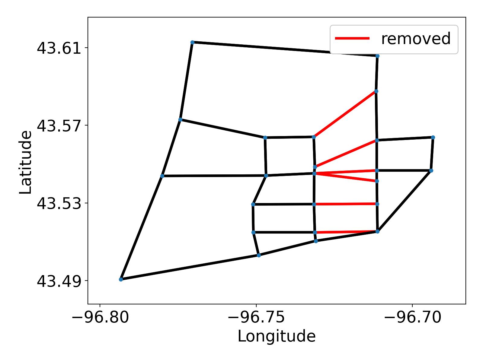
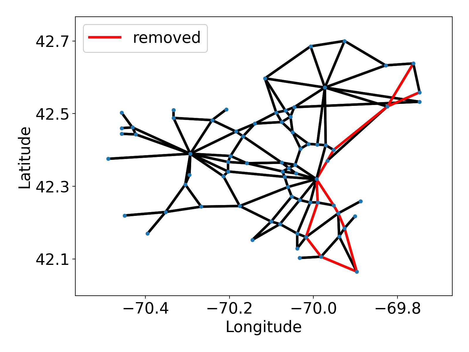
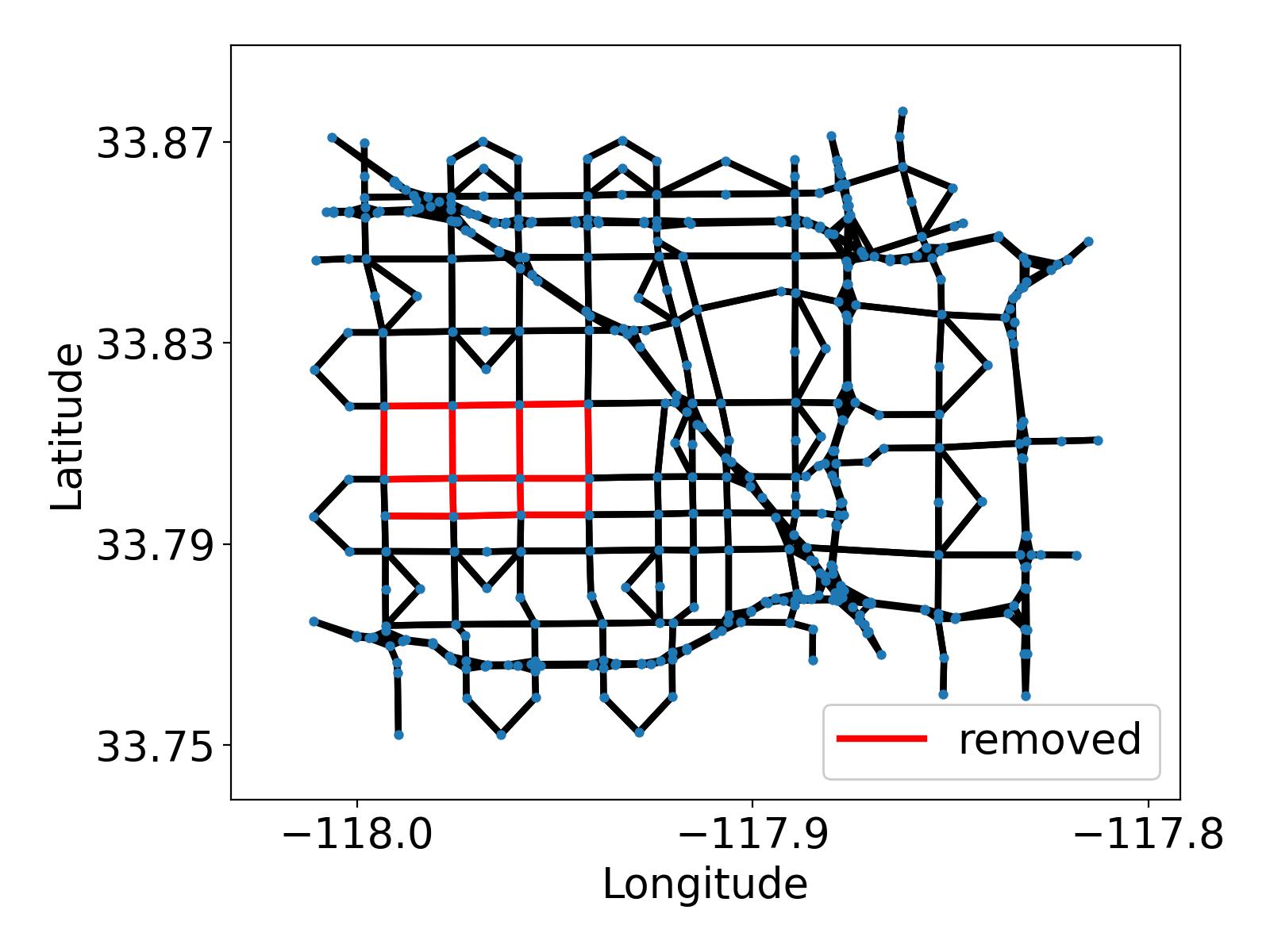
In this experiment, the training and testing datasets both consist of transportation networks where one to three links were randomly removed from a subset of the links. The subset of links is shown in Figure 3. The link removal will create numerous variations to the original transportation systems, and will reflect the real-world scenarios. The training strategies and model architectures remained unchanged as Section 5.1.2. As shown in Table 3, a comparative analysis of predictive accuracy across different models and scenarios reveals that M-HetGAT consistently achieves superior performance. For instance, in the Sioux Falls network, M-HetGAT reduces flow MAEs by 23.2% in the system-optimal scenario and 29.1% in the user equilibrium scenario, outperforming the next best model. Moreover, the improvements in the EMA network are even more significant, with MAE reductions of 51.2% and 55.2%, respectively. These results emphasize the benefits of integrating multi-view modeling and virtual links into the proposed model, which likely enhances its ability to capture and predict complex traffic flow dynamics. Specifically, the model identifies missing links in the networks using a GNN, and the updated node features are processed through both intra-view and inter-view graph attention networks. This approach not only contributes to the model’s generalization capabilities but also enhances its robustness and reliability across diverse network conditions.
| Setting | Metric | Model | Sioux Falls | EMA | Anaheim | |||||||||||
| Car | Truck | Car | Truck | Car | Truck | |||||||||||
| MAE | RMSE | MAE | RMSE | MAE | RMSE | MAE | RMSE | MAE | RMSE | MAE | RMSE | |||||
|
Flow | M-GAT | 5.33 | 6.89 | 3.23 | 4.23 | 0.54 | 0.88 | 0.52 | 0.84 | 3.42 | 4.57 | 0.71 | 1.00 | ||
| M-GCN | 4.00 | 5.23 | 3.16 | 4.12 | 0.72 | 1.23 | 0.58 | 0.96 | 3.45 | 4.68 | 0.62 | 0.88 | ||||
| M-GraphSAGE | 4.53 | 5.92 | 3.14 | 4.14 | 0.39 | 0.65 | 0.39 | 0.63 | 2.63 | 3.67 | 0.46 | 0.69 | ||||
| M-HetGAT | 3.08 | 4.22 | 2.35 | 3.34 | 0.24 | 0.39 | 0.19 | 0.33 | 2.40 | 3.36 | 0.33 | 0.49 | ||||
| Ratio | M-GAT | 4.08% | 5.75% | 2.34% | 3.23% | 1.72% | 2.75% | 1.58% | 2.51% | 2.62% | 3.78% | 0.71% | 1.07% | |||
| M-GCN | 3.03% | 4.18% | 2.31% | 3.08% | 2.23% | 3.51% | 1.98% | 3.25% | 2.74% | 4.14% | 0.82% | 1.19% | ||||
| M-GraphSAGE | 3.40% | 4.63% | 2.29% | 3.09% | 1.19% | 1.93% | 1.26% | 2.07% | 2.78% | 3.79% | 0.97% | 1.25% | ||||
| M-HetGAT | 2.24% | 3.20% | 1.70% | 2.56% | 0.72% | 1.18% | 0.58% | 0.98% | 2.52% | 3.29% | 0.88% | 1.09% | ||||
|
Flow | M-GAT | 4.09 | 5.24 | 3.01 | 3.96 | 0.56 | 0.96 | 0.56 | 0.97 | 3.30 | 4.62 | 0.54 | 0.79 | ||
| M-GCN | 3.91 | 5.05 | 3.12 | 4.14 | 0.83 | 1.39 | 0.78 | 1.34 | 2.85 | 4.22 | 0.56 | 0.87 | ||||
| M-GraphSAGE | 4.22 | 5.52 | 3.08 | 4.04 | 0.48 | 0.86 | 0.45 | 0.83 | 3.02 | 4.30 | 0.72 | 1.05 | ||||
| M-HetGAT | 3.29 | 4.25 | 2.29 | 2.98 | 0.26 | 0.49 | 0.24 | 0.46 | 2.29 | 3.40 | 0.44 | 0.66 | ||||
| Ratio | M-GAT | 3.12% | 4.21% | 2.17% | 2.93% | 1.70% | 3.03% | 1.76% | 3.27% | 4.71% | 6.41% | 1.48% | 1.91% | |||
| M-GCN | 2.97% | 4.00% | 2.29% | 3.13% | 2.47% | 3.88% | 2.24% | 3.37% | 3.32% | 4.90% | 0.93% | 1.44% | ||||
| M-GraphSAGE | 3.29% | 4.65% | 2.29% | 3.14% | 1.41% | 2.58% | 1.35% | 2.51% | 2.89% | 4.17% | 0.78% | 1.16% | ||||
| M-HetGAT | 2.48% | 3.40% | 1.68% | 2.29% | 0.73% | 1.35% | 0.68% | 1.34% | 1.64% | 2.54% | 0.44% | 0.64% | ||||
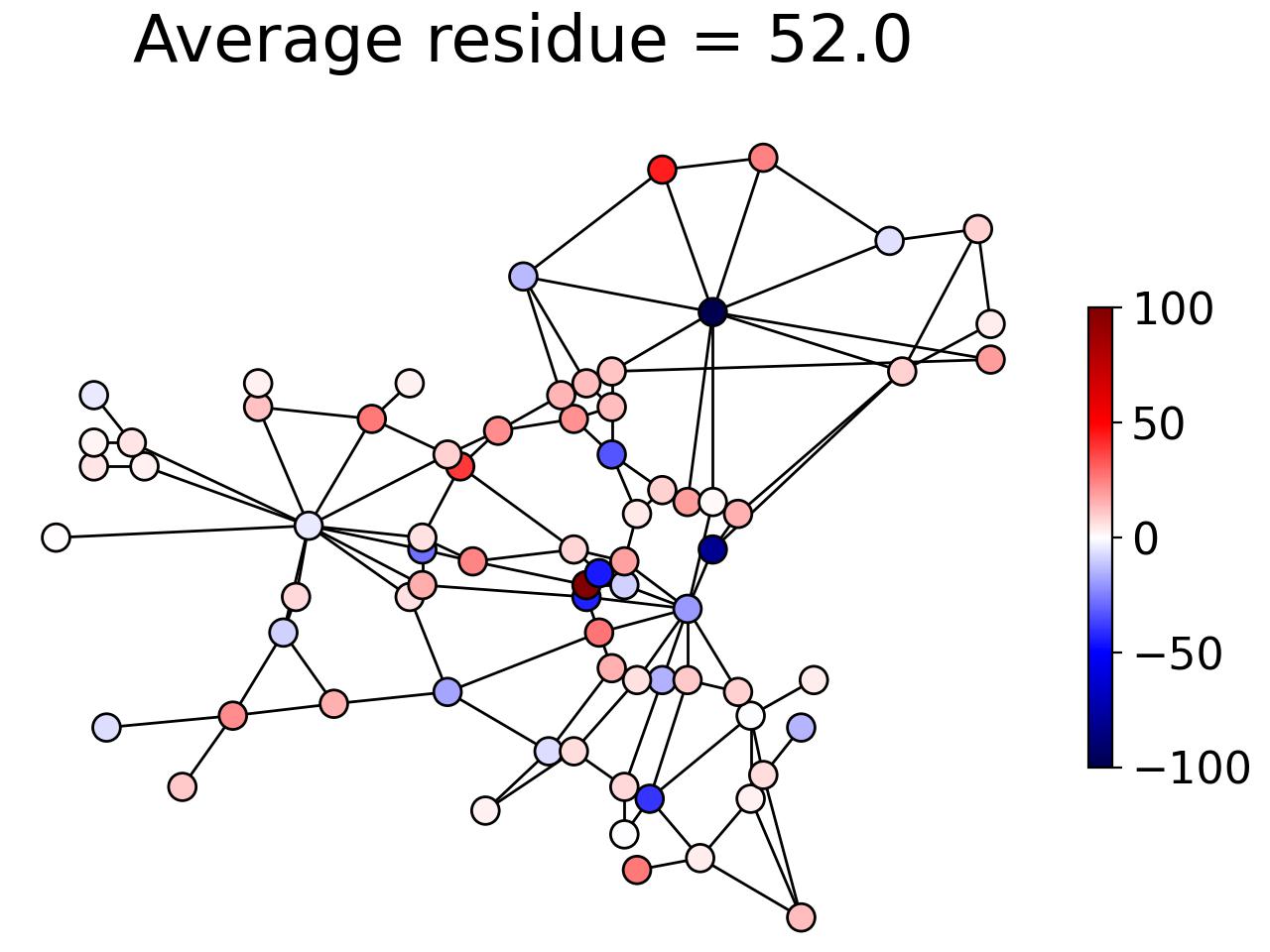
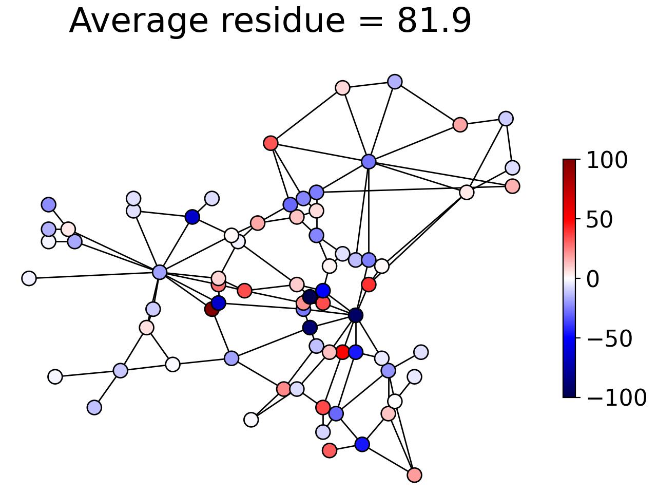
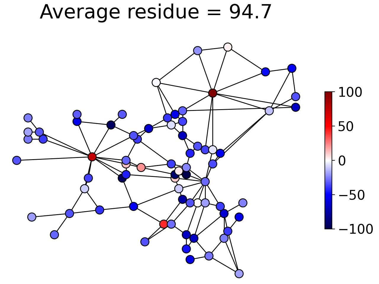
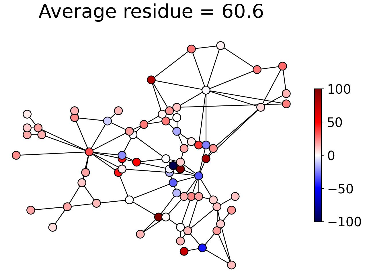
Additionally, Figure 4 visualizes the conservation residues at the node level. Specifically, we show the violation to the conservation low at each node in the EMA network when different models calculates the system optimal flows. As can be seen, our proposed M-HetGAT model demonstrates superior in adheroing to the flow conservation, compared to its homogeneous counterparts, showing a 13% improvement over the next best model. Moreover, the average normalized flow conservation residue relative to the total OD demand is 2.91%. This suggests that the M-HetGAT model not only improves the accuracy of flow predictions but also ensures better compliance with the physical and network constraints.
5.2.2 Out of distribution testing on modified network
In this section, the training set consists of a transportation network where one or two links were randomly removed, whereas the testing set comprises networks with three links randomly removed. However, the training setup and hyperparameters remain identical to those in the previous experiments discussed in Section 5.1.2. The results, as shown in Table 4, indicate that our proposed M-HetGAT model consistently outperforms the baseline models including M-GAT, M-GCN, and M-GraphSAGE, across all networks, under both user equilibrium and system optimal scenarios. To explain further, the graph neural network identifies the missing links in the network, and the updated node features are processed through the intra-view and inter-view graph attention networks. Despite the network topologies are not seen in the training, our model still achieves accurate link flow predictions. This is especially notable compared to homogeneous GNN models, as our M-HetGAT model effectively captures the influence of OD pairs through virtual links. Consequently, it is more expressive and better equipped to model and learn the impact of topological alterations on flow distributions.
| Setting | Metric | Model | Sioux Falls | EMA | Anaheim | |||||||||||
| Car | Truck | Car | Truck | Car | Truck | |||||||||||
| MAE | RMSE | MAE | RMSE | MAE | RMSE | MAE | RMSE | MAE | RMSE | MAE | RMSE | |||||
|
Flow | M-GAT | 8.28 | 11.65 | 7.20 | 9.60 | 0.76 | 1.20 | 0.67 | 1.03 | 2.88 | 4.04 | 0.59 | 0.84 | ||
| M-GCN | 10.05 | 14.14 | 9.53 | 12.90 | 1.23 | 2.13 | 1.24 | 2.02 | 2.82 | 3.92 | 0.63 | 0.94 | ||||
| M-GraphSAGE | 8.03 | 10.89 | 6.14 | 8.26 | 0.78 | 1.29 | 0.80 | 1.31 | 2.87 | 4.06 | 0.38 | 0.57 | ||||
| M-HetGAT | 7.44 | 10.59 | 5.51 | 7.57 | 0.42 | 0.88 | 0.34 | 0.76 | 2.76 | 3.76 | 0.46 | 0.64 | ||||
| Ratio | M-GAT | 5.97% | 8.55% | 5.28% | 7.28% | 2.39% | 3.57% | 2.20% | 3.36% | 3.44% | 4.76% | 0.99% | 1.39% | |||
| M-GCN | 7.18% | 10.00% | 6.59% | 8.75% | 3.91% | 6.19% | 4.02% | 6.16% | 2.52% | 3.74% | 0.78% | 1.17% | ||||
| M-GraphSAGE | 5.90% | 8.36% | 4.37% | 6.01% | 2.35% | 3.64% | 2.40% | 3.70% | 3.03% | 4.31% | 1.01% | 1.29% | ||||
| M-HetGAT | 5.33% | 7.70% | 3.96% | 5.54% | 1.12% | 1.99% | 0.91% | 1.76% | 2.08% | 3.07% | 0.43% | 0.62% | ||||
|
Flow | M-GAT | 6.36 | 8.44 | 5.40 | 7.52 | 1.16 | 1.94 | 1.00 | 1.57 | 4.05 | 5.54 | 0.90 | 1.26 | ||
| M-GCN | 7.53 | 11.30 | 6.79 | 10.11 | 1.59 | 2.44 | 1.39 | 2.21 | 3.31 | 4.73 | 0.63 | 0.96 | ||||
| M-GraphSAGE | 6.57 | 8.70 | 5.36 | 7.00 | 0.85 | 1.44 | 0.84 | 1.37 | 3.00 | 4.33 | 0.52 | 0.81 | ||||
| M-HetGAT | 6.04 | 8.51 | 5.58 | 7.81 | 0.39 | 0.86 | 0.40 | 0.91 | 2.96 | 4.21 | 0.45 | 0.67 | ||||
| Ratio | M-GAT | 5.10% | 7.39% | 4.29% | 6.54% | 3.67% | 5.94% | 3.35% | 5.79% | 3.95% | 6.12% | 1.01% | 1.63% | |||
| M-GCN | 5.91% | 9.47% | 5.14% | 8.24% | 5.11% | 7.65% | 4.73% | 7.36% | 3.28% | 5.40% | 0.96% | 1.46% | ||||
| M-GraphSAGE | 5.07% | 7.19% | 4.02% | 5.66% | 2.66% | 4.66% | 2.78% | 4.94% | 3.00% | 4.35% | 0.89% | 1.30% | ||||
| M-HetGAT | 4.83% | 7.39% | 4.37% | 6.58% | 1.09% | 2.27% | 1.09% | 2.33% | 2.41% | 3.35% | 0.55% | 0.76% | ||||
In addition to prediction accuracy, training time is a critical factor when assessing the efficiency and practicality of machine learning models. The overall computational time can be broken down into three key components: (1) the time spent solving traffic assignment problems, (2) the training time for the GNN model, and (3) the GNN’s inference time. For every 1,000 graphs from the Sioux Falls, EMA, and Anaheim networks, the time required to solve multi-class vehicle TAP is 56.8, 575.2, and 2,612.5 minutes, respectively. In contrast, the training time of the M-HetGAT model for the same graphs is significantly lower, at 26.8, 28.9, and 59.7 minutes, respectively. Furthermore, the inference time for the M-HetGAT is particularly efficient, taking just 0.13, 0.15, and 0.31 minutes, respectively, for the same set of graphs. This breakdown of computational time highlights the overall efficiency of the proposed model in addressing traffic assignment problems.
5.3 Ablation Study
To evaluate the effectiveness of each component within the M-HetGAT framework, we conducted an ablation study by excluding various components of the model one at a time. In particular, we considered five cases: (1) “w/o link feat", which is M-HetGAT without road link features, thereby omitting the consideration of link-specific variations; (2) “w/o OD link", which is M-HetGAT without any OD link, forming a homogeneous graph with only physical links; and (3) “w/o Intra view", which is M-HetGAT after removing intra-view message passing; (4) “w/o Multi-head", which is M-HetGAT with only single head attention mechanism; (5) “w/o conservation", which remove the flow conservation loss in the back propagation. To ensure a comprehensive evaluation, we conducted experiments with all variants across all three networks, under both system optimal scenarios and user equilibrium scenarios. Specifically, we compared the mean absolute error of the link utilization ratio among different configurations. This approach allowed us to identify the impact of each component on the model’s overall performance.
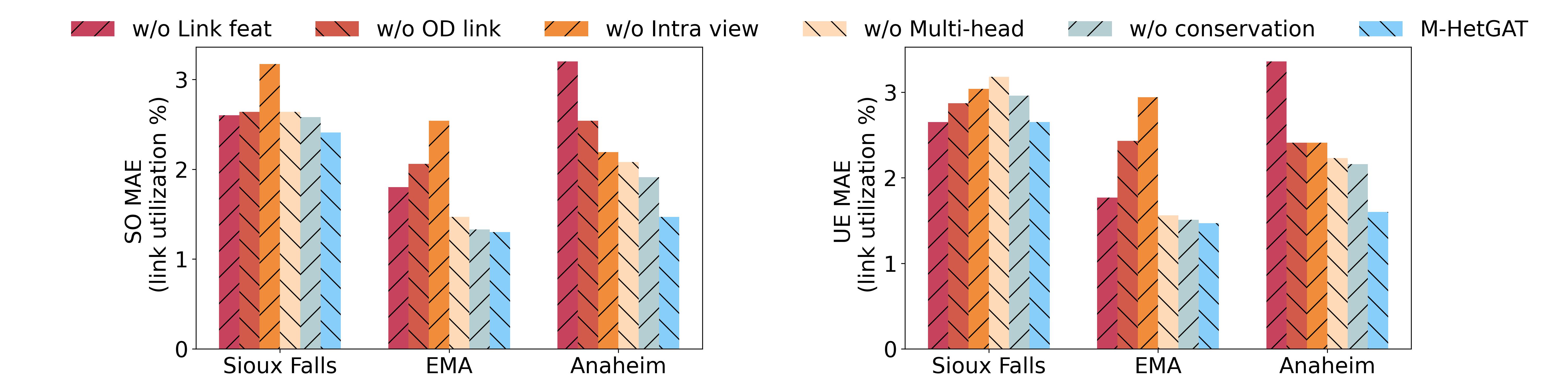
The comparative analysis, illustrated in Figure 5, highlights a degradation in performance across all modified models compared to the complete model, emphasizing the critical contribution of each individual component. Notably, the inclusion of OD links proves to be particularly influential, as their removal results in significant increases in error for flow and link utilization predictions. This can be attributed to the fact that integrating OD links into the M-HetGAT model reduces the need for excessive embedding propagation through road links, thereby enhancing model efficiency.
Furthermore, removing link features from the OD links also leads to a performance decline, underscoring the importance of link features in accurately predicting traffic flow. Similarly, the removal of intra-view message passing and multi-head attention mechanisms from the models also results in decreased performance compared to the full model. Specifically, intra-view message passing, which is designed for multi-class traffic assignment, facilitates the adaptive representation of link features, thereby improving the model’s ability to capture dynamic traffic flow distribution. Additionally, excluding the conservation loss from the overall loss function further degrades performance, indicating that the regularization term plays a crucial role in improving the model’s overall effectiveness.
6 Conclusion and Discussion
This study introduces a novel multi-view heterogeneous graph neural network (M-HetGAT) framework to tackle the computational challenges of multi-class traffic assignment problems in large-scale transportation networks. The framework employs a multi-view graph attention mechanism designed to accommodate different vehicle classes and integrates a conservation-based loss function, ensuring high accuracy in predicting link flows and utilization ratios while maintaining adherence to core traffic flow principles. Comprehensive experiments on urban road networks validate the model’s efficacy and generalizability, showcasing significant improvements in convergence speed and predictive accuracy over conventional graph neural network models. Moreover, the study highlights the model’s ability to address real-world complexities, including varying road accessibility for diverse vehicle classes and dynamic network conditions, such as road closures and topology changes.
The proposed framework serves as a surrogate model capable of significantly accelerating complex optimization tasks in domains such as resource allocation and infrastructure asset management. While the current model is designed for static origin-destination demand data, future research could explore its extension to dynamic demand conditions and real-time traffic updates. Incorporating external influences such as weather, special events, and socio-economic factors may further broaden the model’s practical applicability.
7 Acknowledgment
This work was supported in part by the National Science Foundation under Grant CMMI-1752302.
References
- Nie et al. (2004) Y. Nie, H. Zhang, D.-H. Lee, Models and algorithms for the traffic assignment problem with link capacity constraints, Transportation Research Part B: Methodological 38 (2004) 285–312.
- Seliverstov et al. (2017) Y. A. Seliverstov, S. A. Seliverstov, I. G. Malygin, A. A. Tarantsev, N. V. Shatalova, O. Y. Lukomskaya, I. P. Tishchenko, A. M. Elyashevich, Development of management principles of urban traffic under conditions of information uncertainty, in: Creativity in Intelligent Technologies and Data Science: Second Conference, CIT&DS 2017, Volgograd, Russia, September 12-14, 2017, Proceedings 2, Springer, 2017, pp. 399–418.
- Zou and Chen (2020) Q. Zou, S. Chen, Resilience modeling of interdependent traffic-electric power system subject to hurricanes, Journal of Infrastructure Systems 26 (2020) 04019034.
- Liu and Meidani (2023) T. Liu, H. Meidani, Optimizing seismic retrofit of bridges: Integrating efficient graph neural network surrogates and transportation equity, in: Proceedings of Cyber-Physical Systems and Internet of Things Week 2023, 2023, pp. 367–372.
- Lee et al. (2003) D.-H. Lee, Y. Nie, A. Chen, A conjugate gradient projection algorithm for the traffic assignment problem, Mathematical and computer modelling 37 (2003) 863–878.
- Zhang et al. (2023) Q. Zhang, S. Q. Liu, A. D’Ariano, Bi-objective bi-level optimization for integrating lane-level closure and reversal in redesigning transportation networks, Operational Research 23 (2023) 23.
- Fan et al. (2023) W. Fan, Z. Tang, P. Ye, F. Xiao, J. Zhang, Deep learning-based dynamic traffic assignment with incomplete origin–destination data, Transportation Research Record 2677 (2023) 1340–1356.
- Rahman and Hasan (2023) R. Rahman, S. Hasan, Data-driven traffic assignment: A novel approach for learning traffic flow patterns using graph convolutional neural network, Data Science for Transportation 5 (2023) 11.
- Liu and Meidani (2024) T. Liu, H. Meidani, End-to-end heterogeneous graph neural networks for traffic assignment, Transportation Research Part C: Emerging Technologies 165 (2024) 104695.
- Babazadeh et al. (2020) A. Babazadeh, B. Javani, G. Gentile, M. Florian, Reduced gradient algorithm for user equilibrium traffic assignment problem, Transportmetrica A: Transport Science 16 (2020) 1111–1135.
- Sun and Szeto (2021) S. Sun, W. Szeto, Multi-class stochastic user equilibrium assignment model with ridesharing: Formulation and policy implications, Transportation Research Part A: Policy and Practice 145 (2021) 203–227.
- Xu et al. (2024) Z. Xu, Y. Peng, G. Li, A. Chen, X. Liu, Range-constrained traffic assignment for electric vehicles under heterogeneous range anxiety, Transportation Research Part C: Emerging Technologies 158 (2024) 104419.
- Zhang et al. (2018) Q. Zhang, Q. Yuan, C. Zeng, X. Li, Y. Wei, Missing data reconstruction in remote sensing image with a unified spatial–temporal–spectral deep convolutional neural network, IEEE Transactions on Geoscience and Remote Sensing 56 (2018) 4274–4288.
- Liu and Meidani (2024a) T. Liu, H. Meidani, Graph neural network surrogate for seismic reliability analysis of highway bridge systems, Journal of Infrastructure Systems 30 (2024a) 05024004.
- Liu and Meidani (2024b) T. Liu, H. Meidani, Heterogeneous graph sequence neural networks for dynamic traffic assignment, arXiv preprint arXiv:2408.04131 (2024b).
- Beckmann et al. (1956) M. Beckmann, C. B. McGuire, C. B. Winsten, Studies in the Economics of Transportation, Technical Report, 1956.
- Liu et al. (2020) Y. Liu, C. Lyu, X. Liu, Z. Liu, Automatic feature engineering for bus passenger flow prediction based on modular convolutional neural network, IEEE Transactions on Intelligent Transportation Systems 22 (2020) 2349–2358.
- Hamilton et al. (2017) W. Hamilton, Z. Ying, J. Leskovec, Inductive representation learning on large graphs, Advances in neural information processing systems 30 (2017).
- Veličković et al. (2017) P. Veličković, G. Cucurull, A. Casanova, A. Romero, P. Lio, Y. Bengio, Graph attention networks, arXiv preprint arXiv:1710.10903 (2017).
- Wang et al. (2019) X. Wang, H. Ji, C. Shi, B. Wang, Y. Ye, P. Cui, P. S. Yu, Heterogeneous graph attention network, in: The world wide web conference, 2019, pp. 2022–2032.
- Fu et al. (2020) X. Fu, J. Zhang, Z. Meng, I. King, Magnn: Metapath aggregated graph neural network for heterogeneous graph embedding, in: Proceedings of The Web Conference 2020, 2020, pp. 2331–2341.
- Bar-Gera et al. (2023) H. Bar-Gera, B. Stabler, E. Sall, Transportation networks for research core team, Transportation Network Test Problems. Available online: https://github.com/bstabler/TransportationNetworks (accessed on May 14 2023) (2023).
- Pulugurtha and Jain (2022) S. S. Pulugurtha, R. N. Jain, Passenger car equivalent travel time of a truck, Multimodal Transportation 1 (2022) 100031.
- Fukushima (1984) M. Fukushima, A modified frank-wolfe algorithm for solving the traffic assignment problem, Transportation Research Part B: Methodological 18 (1984) 169–177.
- Paszke et al. (2019) A. Paszke, S. Gross, F. Massa, A. Lerer, J. Bradbury, G. Chanan, T. Killeen, Z. Lin, N. Gimelshein, L. Antiga, et al., Pytorch: An imperative style, high-performance deep learning library, Advances in neural information processing systems 32 (2019).
- Wang et al. (2019) M. Wang, D. Zheng, Z. Ye, Q. Gan, M. Li, X. Song, J. Zhou, C. Ma, L. Yu, Y. Gai, et al., Deep graph library: A graph-centric, highly-performant package for graph neural networks, arXiv preprint arXiv:1909.01315 (2019).
- Liu and Meidani (2023) T. Liu, H. Meidani, Physics-informed neural network for nonlinear structural system identification, in: 14th International Workshop on Structural Health Monitoring: Designing SHM for Sustainability, Maintainability, and Reliability, IWSHM 2023, DEStech Publications, 2023, pp. 3001–3011.
- Rodrigue (2020) J.-P. Rodrigue, The geography of transport systems, Routledge, 2020.