StereoGen: High-quality Stereo Image Generation from a Single Image

Abstract

State-of-the-art supervised stereo matching methods have achieved amazing results on various benchmarks. However, these data-driven methods suffer from generalization to real-world scenarios due to the lack of real-world annotated data. In this paper, we propose StereoGen, a novel pipeline for high-quality stereo image generation. This pipeline utilizes arbitrary single images as left images and pseudo disparities generated by a monocular depth estimation model to synthesize high-quality corresponding right images. Unlike previous methods that fill the occluded area in warped right images using random backgrounds or using convolutions to take nearby pixels selectively, we fine-tune a diffusion inpainting model to recover the background. Images generated by our model possess better details and undamaged semantic structures. Besides, we propose Training-free Confidence Generation and Adaptive Disparity Selection. The former suppresses the negative effect of harmful pseudo ground truth during stereo training, while the latter helps generate a wider disparity distribution and better synthetic images. Experiments show that models trained under our pipeline achieve state-of-the-art zero-shot generalization results among all published methods. The code will be available upon publication of the paper.

1 Introduction

Stereo matching is a fundamental technique in computer vision that estimates depth information by identifying corresponding points between images captured from stereo cameras. By calculating the disparity between matching pixels in the image pair, stereo matching enables the reconstruction of 3D scene structures.

With the advancement of deep learning, stereo matching techniques have shifted from traditional hand-crafted feature matching to data-driven methods [2, 17, 42, 43, 39]. While deep learning-based stereo matching methods have achieved excellent performance on public benchmarks, their data-driven essence brings challenges in generalization to real-world scenarios. As it’s difficult to obtain annotated real-world data in stereo matching, most models are trained on synthetic datasets [21, 38] or limited real-world datasets [28, 29] that may not cover the range of real-world complex scenarios. Many methods have been proposed to alleviate this challenge in the past few years.

One of these methods [46, 18, 6, 3] proposes to learn domain-invariant feature representations from synthetic datasets. However, a generalization gap remains due to the inherent differences between synthetic and real-world data distributions. Another type of these methods [33, 34] is self-supervised learning. This classic method relies on photometric loss from unlabeled stereo images as proxy supervision, taking advantage of the geometric consistency between paired images. Still, it encounters challenges when calculating photometric loss with occlusions, ghosting artifacts, or other ill-posed regions, and large-scale acquisition of unlabeled stereo images remains a nontrivial task.

In recent years, view synthesis techniques [23, 25] have become a mainstream approach in self-supervised stereo matching. These methods generate pseudo stereo images and corresponding pseudo disparity labels from single images or NeRF-rendered scenes. Initially, common strategies [40] use monocular depth estimation models to create pseudo disparity labels from single images, combined with forward warping to generate the right images. However, it faces the challenge of occlusion areas in synthesized right images, typically filled with neighbor pixels [20] or random backgrounds [40], resulting in damaged semantic structure. As techniques advance, generating stereo images directly from NeRF-rendered scenes [35] begins to show distinct advantages. This method enables the flexible generation of stereo images with various disparity ranges while implicitly addressing occlusions in the rendering process. In addition, NeRF-Stereo [35] introduces Ambient Occlusion to measure the confidence of pseudo disparities, further improving training reliability. However, building a NeRF-rendered scene requires capturing multiple viewpoints of the same scene, making it less flexible than earlier single-image-based methods. Moreover, it is restricted to small-scale static scenes, resulting in suboptimal performance in large-scale outdoor scenes.

In this paper, we propose StereoGen, a novel pipeline for high-quality stereo image generation from arbitrary single images. Inspired by Marigold [11], we claim that modern diffusion models, pre-trained on large-scale image datasets, are also easy to transfer to stereo matching. To address the challenge of occlusion areas in synthesized right images, we fine-tune a diffusion inpainting model adapting to the diverse and complex inpainting masks encountered in stereo matching. This model inpaints occlusion areas in synthesized right images, significantly recovering semantic structure and improving image quality, thus enhancing the robustness of model training. Besides, we propose Training-Free Confidence Generation, which derives confidence for pseudo disparities from a pre-trained monocular depth estimation model without additional training. It helps balance disparity loss and photometric loss and suppress the negative effects of harmful labels. To further improve image synthesis quality and obtain a wide disparity range, we propose Adaptive Disparity Selection. This method avoids excessive occlusion or foreground distortion due to large disparity ratios. It also generates large disparity in high-resolution images, helping models adapt to various disparity values.

Experiments demonstrate that our pipeline provides an efficient, straightforward solution for high-quality stereo image generation. Our main contributions can be summarized as follows:

• We propose a novel pipeline StereoGen for high-quality stereo image generation, including a fine-tuned diffusion inpainting model adapting to complex inpainting masks in stereo matching.

• We propose Training-Free Confidence Generation and Adaptive Disparity Selection to improve the reliability of pseudo disparity and image quality.

• We verify that models trained under our pipeline achieve state-of-the-art zero-shot generalization performance with only a synthesized data amount comparable to Scene Flow.

2 Related Work

Deep Stereo Matching. With the advancement of deep learning, learning-based stereo methods have significantly progressed. Methods [2, 30] starting from DispNet [21], and GC-Net [12] utilize stacked CNNs to aggregate cost volume in a pre-defined disparity range. In recent years, methods based on iterative optimization [17, 42, 43, 44] have taken inspiration from RAFT [32] to predict arbitrary disparity in iterations. There are also some methods based on transformers [15, 8] that capture long-range correspondence between features and aggregate cost volume globally.

Zero-shot Generalization in Stereo Matching. Although deep stereo matching methods have significantly progressed, they suffer from generalization to real-world scenarios. DSMNet [46] proposes a domain normalization layer and a non-local graph-based filter to regularize data distribution and extract robust feature representations. GraftNet [18] proposes to leverage the feature of a model trained on large-scale datasets.  [6] proposes ITSA to automatically restrict shortcut-related information. Rao et al. [26] design an effective masked representation inspired by masked representation learning and multi-task learning. Another branch of methods uses unlabeled real-world images for self-supervised learning. Luo et al. [20] first propose to train stereo matching models using a single view on the KITTI domain.  [40] uses a collection of single images to generate stereo images and train stereo matching models from scratch. NeRF-Stereo [35] leverages neural rendering solutions to generate stereo images from rendered scenes.

Diffusion Models for Image Synthesis. Denoising Diffusion Probabilistic Models (DDPMs) [9] have made a significant breakthrough in image synthesis, which describes the process of data generation through a sequence of gradual noise addition and removal. In recent years, Latent Diffusion Models (LDM) [27] perform the diffusion steps in the latent space, which reduces computational requirements compared to previous methods. ControlNet [47] adds spatial conditioning controls to large, pre-trained text-to-image diffusion models to control image generation. Repaint [19] proposes an inpainting method that solely leverages an off-the-shelf unconditionally trained DDPM.

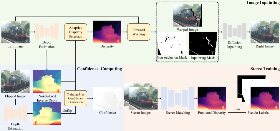
Figure 2: Overview of our StereoGen pipeline. The monocular depth estimation model inferences the normalized inverse depth from the left image, and our Training-Free Confidence Generation (Sec. 3.3) and Adaptive Disparity Selection (Sec. 3.4) modules extract the confidence and the pseudo disparity from it. Then the pipeline uses forward warping to obtain the warped image and corresponding masks, which will be sent into the diffusion inpainting model (Sec. 3.2) to synthesize the right image.

3 Method

In this section, we present the overview of our StereoGen pipeline (Fig. 2) and details of our proposed modules.

3.1 Overview

Given a single image as the left image $\mathbf{I}_{l}$, we first send it to the monocular depth estimation model (we use Depth Anything V2 [45]) to obtain the normalized inverse depth $\mathbf{D}$. Then we convert it to the corresponding disparity $\mathbf{d}$ using our Adaptive Disparity Selection (ADS) module. We use the forward warping method from  [40] to extract the warped image $\tilde{\mathbf{I}}_{r}$, the non-occlusion mask $\mathbf{M}_{noc}$ (pixels only visible in $\mathbf{I}_{l}$), and the inpainting mask $\mathbf{M}_{inp}$ (pixels invisible in $\mathbf{I}_{l}$). $\tilde{\mathbf{I}}_{r}$ and $\mathbf{M}_{inp}$ are sent into the diffusion inpainting model to synthesize the high-quality right image $\mathbf{I}_{r}$. Besides, to compute the confidence of the pseudo disparity, we design the Training-Free Confidence Generation (TCG) module to obtain the confidence $\mathbf{C}$. At last, we use synthesized stereo images and corresponding pseudo labels to train stereo matching models.

3.2 Image Inpainting

We fine-tune our diffusion inpainting model based on the pre-trained Stable Diffusion (SD) model [27]. We can directly use the inpainting version corresponding to this pre-trained model for image inpainting. However, there exist differences between standard image inpainting and image inpainting in stereo matching.

First, there is no text guidance. As a text-to-image model, the SD model is trained on text-conditioned and unconditioned data. Still, no reliable text prompt guides the model in inpainting occlusion areas in stereo matching. Second, unlike standard image inpainting which typically replaces an object or a portion of it, occlusion masks in stereo matching have diverse and complex shapes. Consequently, directly using a pre-trained model yields suboptimal results, making fine-tuning necessary for effective performance.

Fine-tuning Protocol. For fine-tuning, we collect synthetic stereo datasets like Scene Flow [21] with dense disparity maps as ground truth. The reason is the same as Marigold [11]: only synthetic data has inherently dense and complete ground truth, allowing us to warp every pixel. Besides, synthetic data has the cleanest images without noise to disturb training. Given a warped image $\tilde{\mathbf{I}}_{r}$, an inpainting mask $\mathbf{M}_{inp}$, and a right image $\mathbf{I}_{r}$, we take the frozen Variational Auto-Encoder (VAE) [13] to encode $\tilde{\mathbf{I}}_{r}$ and $\mathbf{I}_{r}$ into the latent space. For the inpainting mask $\mathbf{M}_{inp}$, we resize it into the same resolution of the latent space. Then, we sample a Gaussian noise $\mathbf{\epsilon}$ and add it to the latent right image. At last, we concatenate these latent features and the resized inpainting mask as the input of the U-Net. The U-Net outputs a noise prediction $\tilde{\mathbf{\epsilon}}$, and we use an L2 loss to optimize the network:

$$\mathcal{L}_{u}=||\tilde{\mathbf{\epsilon}}-\mathbf{\epsilon}||^{2}_{2}$$ (1)

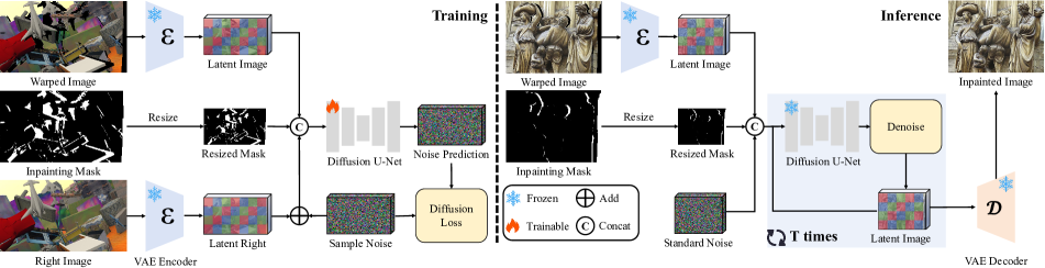
Figure 3: Overview of our diffusion inpainting protocol. During training, we freeze VAE and only fine-tune U-Net.

Inference Protocol. Given a warped image $\tilde{\mathbf{I}}_{r}$, and an inpainting mask $\mathbf{M}_{inp}$, we first encode them into the latent space same as the training protocol. Then we sample a standard Gaussian noise as the initial latent right image. We concatenate them as the input of the U-Net. During inference, we denoise it in the latent space. After executing the schedule of $\mathbf{T}$ steps, we use the VAE decoder to obtain the denoised image $\mathbf{I}_{d}$ and get the final inpainted image $\mathbf{I}_{r}$:

$$\mathbf{I}_{r}=\mathbf{M}_{inp}\odot\mathbf{I}_{d}+(1-\mathbf{M}_{inp})\odot\tilde{\mathbf{I}}_{r}$$ (2)

3.3 Training-Free Confidence Generation

It’s difficult to obtain accurate confidence in a depth prediction from previous monocular depth estimation models without extra training or auxiliary modules. Even without training, some post-processing methods need gradients [10] or probability distributions [41] to measure uncertainty.

With the development of deep learning, modern monocular depth estimation models tend to predict relative depth, usually represented by inverse depth in the disparity space. This depth measures the relative distance between pixels, independent of camera parameters. Therefore, we can assume that if we flip an image horizontally, the relative depth between pixels in the prediction remains unchanged.

Given a left image $\mathbf{I}_{l}$, we use the horizontal flip operation $\mathbf{H(x)}$ to get the flipped image $\mathbf{I}_{l}^{\prime}$. Then we separately send them to the monocular depth estimation model to get the relative depth maps. Because we use Depth Anything V2 [45] as our model, which has no constraint range for its predictions, we normalize these predictions into the normalized inverse depth maps $\mathbf{D}$ and $\mathbf{D}^{\prime}$. Now we measure the confidence $\mathbf{C}$ of $\mathbf{D}$:

$$\mathbf{u}= 1-|\mathbf{D}-\mathbf{H}^{-1}(\mathbf{D}^{\prime})|$$ (3)

$$\mathbf{C}= \frac{\mathbf{u}-\min(\mathbf{u})}{\max(\mathbf{u})-\min(\mathbf{u})}$$

As shown in Fig. 4, low-confidence areas are often located at edge, textureless, and thin object areas, which are also ill-posed regions in stereo matching. These harmful labels will be suppressed during stereo training.

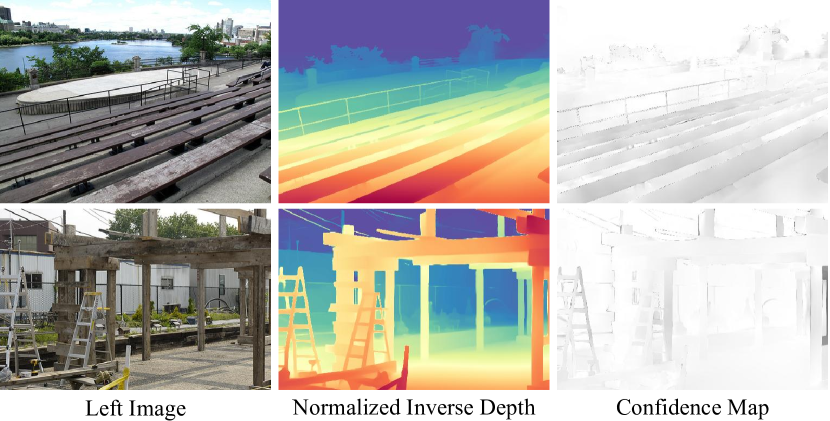
Figure 4: Visualization of confidence map.

3.4 Adaptive Disparity Selection

The previous method MfS-Stereo [40] generates the disparity map by sampling the max disparity value uniformly from $[d_{min},d_{max}]$. This fixed-range method brings some issues.

First, when the resolution of an image is small, the ratio of disparity to image width may be slightly large, leading to foreground distortion in forward warping or failure inference of the diffusion inpainting model due to excessive occlusion. Second, when the resolution of an image is large, the ratio of disparity to image width may be slightly small, leading to no difference between the left and right images.

Therefore, we convert the normalized inverse depth map $\mathbf{D}$ into the disparity map $\mathbf{d}$ by multiplying $\mathbf{s}\cdot\mathbf{w}$, where $\mathbf{w}$ is the width of the image, and the scale $s$ can be sampled from follows:

$$\mathbf{s}\in\left\{\begin{array}[]{lll}(\mathbf{c}-2\mathbf{r},\mathbf{c}-\mathbf{r}),&\mathbf{p}=\mathbf{p}_{s}\\ (\mathbf{c}-\mathbf{r},\mathbf{c}+\mathbf{r}),&\mathbf{p}=\mathbf{p}_{c}\\ (\mathbf{c}+\mathbf{r},\mathbf{c}+2\mathbf{r}),&\mathbf{p}=\mathbf{p}_{l}\end{array}\right.$$ (4)

where $\mathbf{c}$ is the center, $\mathbf{r}$ is the radius, and $\mathbf{p}_{i}$ ($i\in\{s,c,l\}$) is the probability. This sampling method ensures that high-quality warped images can be generated in most cases, while also generating some cases with extreme disparity values for later stereo training. Because the collection of single-image datasets has different resolutions, the disparity range sampled based on width can also be large, covering almost all conditions.

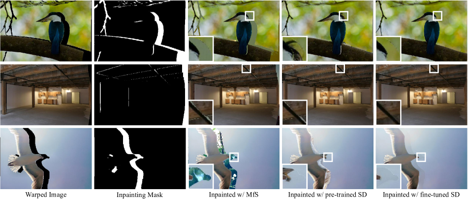
Figure 5: Visualization of different inpainting methods. Pixels inpainted with our fine-tuned SD model have the least noise and the semantic structure closest to the background.

3.5 Stereo Training

Given a stereo pair ($\mathbf{I}_{l}$, $\mathbf{I}_{r}$), a disparity map $\mathbf{d}$, a confidence map $\mathbf{C}$, a non-occlusion mask $\mathbf{M}_{noc}$, an inpainting mask $\mathbf{M}_{inp}$, and an estimated disparity map $\tilde{\mathbf{d}}$, we train stereo matching models with our proposed StereoGen loss.

Disparity Loss. We use the same L1 loss as previous supervised stereo matching methods:

$$\mathcal{L}_{d}=||\tilde{\mathbf{d}}-\mathbf{d}||_{1}$$ (5)

For iterative optimization methods, we keep the same iterative weights as they do.

Non-occlusion Photometric Loss. We backward warp $\mathbf{I}_{r}$ according to the estimated disparity $\tilde{\mathbf{d}}$ and obtain $\mathbf{I}_{l}^{r}$. Then we calculate the ordinary photometric loss:

$$\mathcal{L}_{p}=\beta\cdot\frac{1-SSIM(\mathbf{I}_{l},\mathbf{I}_{l}^{r})}{2}+(1-\beta)\cdot||\mathbf{I}_{l}-\mathbf{I}_{l}^{r}||_{1}$$ (6)

It should be noted that $\mathbf{I}_{l}^{r}$ contains pixels inpainted by the diffusion inpainting model. We need to filter them by backward warping $1-\mathbf{M}_{inp}$ to obtain $\tilde{\mathbf{M}}_{inp}^{r}$. Besides, $\mathbf{I_{l}^{r}}$ contains ghost artifacts caused by backward warping, and we can also use the non-occlusion mask $\mathbf{M}_{noc}$ to filter them. Thus, we compute our non-occlusion photometric loss as follows:

$$\mathcal{L}_{np}=\mathbf{M}_{noc}\odot\tilde{\mathbf{M}}_{inp}^{r}\odot\mathcal{L}_{p}$$ (7)

StereoGen Loss. The above two terms are summed as:

$$\mathcal{L}_{SG}=\mathbf{C}\odot\mathcal{L}_{d}+\mu\cdot(1-\mathbf{C})\odot\mathcal{L}_{np}$$ (8)

where $\mathbf{C}$ is the weight balancing the influence of these two terms.

4 Experiments

In this section, we introduce our implementation details, evaluation datasets, ablation study, and final results.

Baseline	ADS	Inpainting	TCG	$\mathcal{L}_{np}$	KITTI-15 All		Midd-T (H) Noc		ETH3D Noc
					EPE	>3px	EPE	>2px	EPE	>1px
✓					1.52	4.89	2.71	8.41	0.25	2.38
	✓				1.24	4.84	2.28	7.46	0.28	2.27
		✓			1.44	4.85	2.34	7.59	0.23	1.92
			✓		1.09	4.78	2.13	7.27	0.27	2.16
	✓	✓			1.06	4.74	2.26	6.68	0.23	2.05
	✓	✓	✓		1.05	4.71	2.34	7.33	0.23	2.01
	✓	✓	✓	✓	1.04	4.73	2.09	7.07	0.22	1.90

Table 1: Ablation study of proposed modules trained with IGEV-Stereo [43]. Baseline denotes that we train the model under the pipeline in  [40]. ADS denotes our Adaptive Disparity Selection module and TCG denotes our Training-free Confidence Generation module. Bold: Best. Underline: Second best.

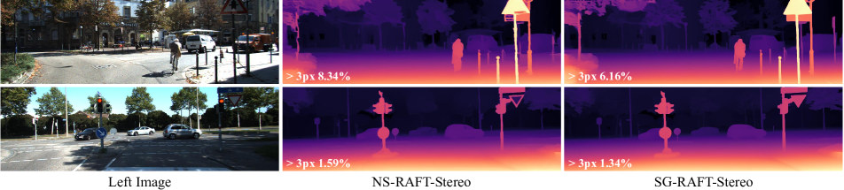
Figure 6: Visualization of KITTI 2015.

4.1 Implementation Details

All experiments are implemented with PyTorch on NVIDIA RTX 4090 GPUs.

Diffusion Inpainting Model Fine-tuning. We utilize the Stable Diffusion V2 Inpainting model [27] as our model. We disable text conditioning and apply the DDPM noise scheduler [9] with 1,000 diffusion steps. We use a collection of synthetic stereo datasets including Tartan Air [38], CREStereo Dataset [14], Scene Flow [21], VKITTI 2 [1], etc. Fine-tuning our model takes 50K steps with a batch size of 32 (we accumulate gradients for 4 steps). We use the AdamW optimizer and the one-cycle learning rate schedule with a learning rate of 2e-5. Besides, we apply a crop size of $512\times 512$ and symmetric color augmentation to the training data.

Stereo Image Generation. We apply the DDIM scheduler [31] and sample 50 steps during diffusion inpainting inference. Following MfS-Stereo [40], we sample images from Depth in the Wild [4], COCO 2017 [16], DIODE [36], ADE20K [48], and Mapillary Vistas [24]. Due to the high quality of the generated images, we only randomly sample 35K to form a dataset called MfS35K. For disparity generation, we set $\mathbf{c}=0.1$, $\mathbf{r}=0.05$, $\mathbf{p}_{c}=0.8$, and $\mathbf{p}_{s}=\mathbf{p}_{l}=0.1$.

Stereo Matching Model Training. We utilize RAFT-Stereo [17] and IGEV-Stereo [43] as our models. We train all models on our MfS35K dataset with a batch size of 8 and a crop size of $384\times 512$.

Method	KITTI-15 All		Midd-T (H) Noc		ETH3D Noc
	EPE	>3px	EPE	>2px	EPE	>1px
Pre-trained	1.18	4.77	2.27	7.21	0.25	1.90
Fine-tuned	1.06	4.74	2.26	6.68	0.23	2.05

Table 2: Ablation study of diffusion inpainting models.

We follow all the source code’s settings and run 200K steps for training from scratch. Besides, we keep the data augmentation from RAFT-Stereo and add Gaussian augmentation on the right image from MfS-Stereo [40]. We use 22 update iterations during training and 32 update iterations during evaluation. For StereoGen loss, we set $\beta=0.85,\mu=0.1$ same as NeRF-Stereo [35].

4.2 Evaluation Datasets

KITTI 2015 [22] contains 200 training pairs with lidar ground truth for outdoor driving scenarios. ETH3D [29] contains 27 training pairs of grayscale images, including outdoor and indoor scenarios. For Middlebury [28], we choose the Middlebury V3 Benchmark Training Set (Midd-T), which contains 15 training pairs for high-resolution indoor scenarios. We also use other Middlebury sets like 2014 and 2021 for visualization. During the evaluation, we calculate the endpoint error (EPE) and the percentage of pixels with errors greater than a threshold $\tau$.

4.3 Ablation Study

In this section, we evaluate models with different settings to verify the effectiveness of our proposed pipeline.

Figure 7: Visualization of different disparity selection.

Effectiveness of proposed modules. Tab.  1 shows the ablation study of our proposed modules, Adaptive Disparity Selection (ADS), Inpainting, and Training-free Confidence Generation (TCG). By adding ADS or TCG to the baseline, we observe a notable improvement across the datasets, particularly a reduction in EPE for KITTI-15 and Midd-T. The former expands the disparity selection range, enhancing the model’s ability to handle large disparities. The latter suppresses unreliable labels, particularly in edges and textureless regions. However, when only adding Inpainting, the improvements are slight. This result supports our hypothesis that the fixed-range disparity selection in  [40] brings issues like foreground distortion. As shown in Fig.  7, the large disparity ratio leads to separation and distortion in the foreground and the ineffectiveness of the diffusion inpainting model. When ADS is combined with inpainting, we observe a significant performance boost across all datasets.

Method	KITTI-15		Middlebury				ETH3D
	>3px		F (>2px Noc)		H (>2px Noc)		>1px
	All	Noc	$\mathbf{D}$ <192	$\mathbf{D}$ <All	$\mathbf{D}$ <192	$\mathbf{D}$ <All	All	Noc
NS-IGEV-Stereo	5.88	5.58	15.89	27.91	8.55	10.67	4.02	3.58
SG-IGEV-Stereo (Ours)	4.73	4.57	13.03	26.78	4.73	7.07	2.64	1.90
NS-RAFT-Stereo∗ [35]	5.41	5.23	16.61	12.04	6.40	6.45	2.95	2.55
NS-RAFT-Stereo	5.65	5.44	15.05	13.41	9.09	9.44	3.30	2.79
SG-RAFT-Stereo (Ours)	4.53	4.33	9.51	8.36	4.21	4.45	2.75	2.13

Table 3: Comparision with NeRF-Stereo [35]. Models are trained with the same augmentation. Exception: $*$ official weights.

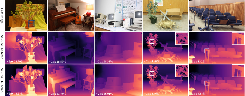
Figure 8: Visualization of Middlebury, including Midd-T, 2014 and 2021.

When ADS, Inpainting, and TCG are all added to the baseline, the performance generally improves compared to previous configurations. However, while TCG suppresses harmful labels in ill-posed regions, it also reduces weight loss for these regions, limiting the model’s ability to learn from them. This limitation can lead to decreased performance on datasets like Middlebury, where these regions are common. To address this issue, we introduce the final SG Loss, which balances $\mathcal{L}_{d}$ and $\mathcal{L}_{np}$. This loss enables the model to maintain robustness and perform best across different datasets.

Effectiveness of fine-tuned inpainting model. Fig.  5 shows a visual comparison between three inpainting methods: MfS [40], a pre-trained SD model, and a fine-tuned SD model. Pixels inpainted with our fine-tuned SD model have the least noise and closest semantic structure to the background. It’s evident in the zoomed-in areas, where the fine-tuned SD model maintains semantic consistency and minimizes ghost artifacts. As shown in Tab.  2, the fine-tuned SD model performs better across all datasets. These results suggest that fine-tuning enables the inpainting model to better capture the semantic structure of the background, resulting in inpainted images with lower noise and better alignment with the original scene content.

4.4 Comparison with NeRF-Stereo

We compare our method with NeRF-Stereo [35], the state-of-the-art method for generating stereo images. As shown in Tab.  3, we train RAFT-Stereo [17] and IGEV-Stereo [43] using these two methods respectively. All models are trained with our same data augmentation, except for NS-RAFT-Stereo^∗, which we directly evaluate with official weights. Besides, the official code of IGEV-Stereo limits the supervised range of $\mathcal{L}_{d}$ to 192, so we divide the Midd-T table into two parts based on disparity. This split method can also show the models’ ability to handle the background in Midd-T.

We note that using our data augmentation, the re-trained NS-RAFT-Stereo does not perform better than the official weights, indicating that the improvement of our model does not solely rely on data augmentation. Compared to NS-RAFT-Stereo^∗ and SG-RAFT-Stereo, SG-RAFT-Stereo has an average improvement of over 20%. Besides, our model performs better in the background, with only a 10$\%$ drop in the part of Midd-T (F) where $\mathbf{D}<192$, while NS-RAFT-Stereo^∗ shows a greater decrease. The reason may be that the Nerf-Stereo’s dataset is reconstructed from NeRF [23], and the reconstruction details of far objects are not good enough.

Method	KITTI-15		Midd-T						ETH3D
	>3px		F (>2px)		H (>2px)		Q (>2px)		>1px
	All	Noc	All	Noc	All	Noc	All	Noc	All	Noc
Training Set	Scene Flow with GT
DSMNet [46]	5.50	5.19	41.96	38.54	18.74	14.49	13.75	9.44	4.03	3.62
CFNet [30]	5.99	5.79	35.21	30.05	21.99	17.69	14.21	10.51	6.08	5.48
Graft-PSMNet [18]	5.34	5.00	39.92	36.30	17.65	13.36	13.92	9.23	11.43	10.70
ITSA-PSMNet [6]	5.83	5.62	39.89	36.81	18.71	14.91	13.36	9.67	10.34	9.77
ITSA-GwcNet [6]	5.45	5.28	38.77	35.58	17.13	13.67	12.98	9.32	7.45	7.13
ITSA-CFNet [6]	4.73	4.67	34.01	30.14	16.48	12.32	12.28	8.54	5.43	5.17
HVT-PSMNet [3]	4.84	4.63	40.74	37.60	15.66	12.55	10.12	7.00	6.07	5.65
RAFT-Stereo [17]	5.47	5.27	15.63	11.94	11.20	8.66	10.25	7.44	2.60	2.29
IGEV-Stereo [43]	6.03	5.76	30.94	28.98	11.9	9.45	8.88	6.20	4.04	3.60
NMRF-Stereo [7]	5.31	5.14	37.63	35.25	13.36	10.90	7.87	5.07	3.80	3.48
Mocha-Stereo [5]	5.97	5.73	30.23	28.26	10.18	9.45	7.96	4.87	4.02	3.47
Training Set	Real-world data without GT
MfS-PSMNet [40]	5.18	4.91	26.42	20.91	17.56	13.45	12.07	9.09	8.17	7.44
NS-RAFT-Stereo [35]	5.41	5.23	16.38	12.04	9.70	6.45	8.09	4.85	2.95	2.55
SG-IGEV-Stereo (Ours)	4.73	4.57	29.47	26.78	9.71	7.07	7.07	4.46	2.64	1.90
SG-IGEV-Stereo∗ (Ours)	4.89	4.73	18.83	14.87	8.45	5.54	6.99	4.38	2.85	2.00
SG-RAFT-Stereo (Ours)	4.53	4.33	12.40	8.36	7.86	4.45	7.24	4.50	2.75	2.13

Table 4: Zero-shot generalization benchmark. We evaluate all models using official weights. SG-IGEV-Stereo^∗ denotes that we expand the supervised range of $\mathcal{L}_{d}$ when training this model, same as RAFT-Stereo [17]. We highlight first, second, third bests.

Finally, we show the visualization of SG-RAFT-Stereo and NS-RAFT-Stereo (using official weights). As shown in Fig.  6, SG-RAFT-Stereo shows an improvement over NS-RAFT-Stereo in KITTI 2015. Moreover, Fig.  8 shows some failed examples of NS-RAFT-Stereo, such as textureless and dark regions, our SG-RAFT-Stereo can easily handle and bring an improvement of over 40%. Our model also performs better in detailed regions, like plants and holes.

4.5 Zero-shot Generalization Benchmark

Following NeRF-Stereo [35], we construct a zero-shot generalization benchmark to compare our models with the state-of-the-art methods. We only collect methods that have published official weights and evaluate them in the same environment. Certainly, we evaluate all methods with the entire disparity range. For IGEV-Stereo [43], we train two versions under our pipeline. One uses the original code setting for disparity supervision, while the other expands the supervised range, consistent with RAFT-Stereo [17].

As shown in Tab.  4, our models demonstrate state-of-the-art zero-shot generalization performance across multiple datasets under both Scene Flow with GT and Real-world data without GT settings. Notably, SG-RAFT-Stereo achieves the best or near-best results on the KITTI-15 and Middlebury datasets, especially excelling in handling complex, real-world scenes. Besides, SG-RAFT-Stereo is the first to achieve a percentage error less than 10$\%$ in the Midd-T (F >2px) Noc regions across these dataset settings.

SG-IGEV-Stereo^∗, with an expanded supervised range of $\mathcal{L}_{d}$, shows improved results on Middlebury’s large-disparity scenarios compared to SG-IGEV-Stereo, although it lead to a slight performance trade-off on other datasets.

5 Conclusion

We propose StereoGen, a novel pipeline for high-quality stereo image generation from arbitrary single images. The fine-tuned diffusion inpainting model can adapt to complex inpainting masks in warped right images and recover background details. To handle harmful pseudo labels, the Training-free Confidence Generation module utilizes the spatial invariance of relative depth to compute confidence that can suppress uncertain labels and balance loss. Besides, the Adaptive Disparity Selection module helps generate a wider disparity distribution while avoiding foreground distortion due to the large disparity ratios. Finally, experiments demonstrate that models trained under our pipeline achieve state-of-the-art zero-shot generalization performance across various datasets.

Limitations. The fine-tuned diffusion inpainting model still fails in some complex scenarios, and there may be some color inconsistency due to synthetic datasets fine-tuning. Besides, the forward warping method performs poorly in some ill-posed regions, like transparent areas, and net-like objects. These limitations can become a good research direction in the future.

Supplementary Material

Method	KITTI-15		Midd-T (H)		ETH3D
	EPE	>3px	EPE	>2px	EPE	>1px
$\mathcal{L}_{p}$	1.03	4.77	0.90	4.95	0.25	2.09
$(1-\mathbf{C})*\mathcal{L}_{p}$	1.03	4.76	0.85	4.81	0.25	2.08
$(1-\mathbf{C})*\mathcal{L}_{np}$	1.02	4.53	0.79	4.45	0.23	2.13

Table 5: Analysis of StereoGen loss. The method default uses $\mathcal{L}_{d}$, and we discuss the impact of loss combinations based on it.

6 Details of Image Synthesis

In this section, we discuss some details of our method.

Image Resolution. The source code of Depth Anything V2 [45] and Stable Diffusion V2 [27] limits the input image resolution, which may cause deformation of objects in the image. Therefore, we do not resize the image during inferencing normalized inverse depth and right image, but instead use padding operations to make the image resolution meet the model requirements. For example, we pad images to ensure that their length and width can be divided by 14 when using Depth Anything V2. Besides, there may not be enough GPU memory for inference for some high-resolution images, especially those in Mapillary Vistas [24]. We first downscale them proportionally to half or quarter resolution, then upscale them after inference.

Forward Warping. We use the source code of MfS-Stereo [40] to implement forward warping, including non-occlusion calculation and depth sharpening. However, we find some issues when using the diffusion model to inpaint the image. First, although modern monocular depth estimation models have developed significantly, there are still some cases where depth edges cannot align with object edges. This results in the edges of foreground objects remaining in their original positions after forward warping. Second, the inpainting mask and warped foreground objects are too close, causing the diffusion model to be misled by the foreground during inference. We use a simple method to alleviate these two issues. Specifically, we use the dilate function in OpenCV to inflate the pseudo disparity. This operation makes foreground objects and surrounding background pixels move together during forward warping. When inpainting, the mask, and the foreground will be separated by background pixels to reduce misleading information. It is worth noting that with this operation, the pre-trained diffusion model still has many cases of inpainting ghost artifacts and noise (Fig.  5), which can only be solved by the fine-tuned diffusion model.

7 StereoGen Loss Analysis

In this section, we discuss the impact of loss combinations.

In Sec.  3.5, we propose the non-occlusion photometric loss $\mathcal{L}_{np}$, and the weighted final loss $\mathcal{L}_{SG}$, but we haven’t discussed in detail the impact of each part on stereo training in the paper. As shown in Tab.  5, the methods from top to bottom represent adding the ordinary photometric loss $\mathcal{L}_{p}$, the $\mathcal{L}_{p}$ with the weight $1-\mathbf{C}$, and the $\mathcal{L}_{np}$ with the weight $1-\mathbf{C}$. Adding $\mathcal{L}_{p}$ performs the worst across all datasets. On the one hand, it lacks a balanced weight; on the other hand, it does not address the issues of ghost artifacts and inpainting pixels. Therefore, after introducing the weight, the performance is improved. Furthermore, the performance is best after masks filter out ghost artifacts and inpainting pixels.

8 More Comparisons with NeRF-Stereo

In this section, we present more comparisons with NeRF-Stereo [35], including details of Midd-T benchmark, visualization of ETH3D, and zero-shot generalization performance in DrivingStereo.

For Midd-T, we present every sample’s performance in Tab.  6. Compared with NS-RAFT-Stereo [35], our SG-RAFT-Stereo has improved in almost all samples. For some samples with poor NS-RAFT-Stereo performance, our model achieves an improvement of nearly 50%.

For ETH3D, we show the visualization of NS-RAFT-Stereo and SG-RAFT-Stereo. As shown in Fig.  9, our SG-RAFT-Stereo exhibits smoother and more accurate disparity maps, with reduced artifacts and noise. For example, in the second row, our model eliminates the large disparity artifacts visible in NS-RAFT-Stereo, particularly in the central dark region. In the third row, the fine structures of the tree-like object are better preserved.

Besides, we evaluate these two models on the DrivingStereo dataset under different weather. As shown in Tab.  7, SG-RAFT-Stereo outperforms NS-RAFT-Stereo across all weather except rainy weather. Both models perform poorly under rainy weather, indicating that it’s a direction for further optimization. Besides, SG-RAFT-Stereo significantly improves under foggy weather, reducing errors from 18.18% to 8.66% at full resolution and from 3.41% to 1.70% at half resolution. Foggy scenarios often suffer from low contrast and visibility, and SG-RAFT-Stereo handles these challenges significantly better. As shown in Fig.  10, under extreme weather conditions, NS-RAFT-Stereo almost fails to predict large textureless regions, but SG-RAFT-Stereo can predict complete ground and walls successfully. Moreover, SG-RAFT-Stereo performs better in segmenting thin, tree-like objects and blurry backgrounds.

Method	Adi.	ArtL	Jad.	Mot.	Mot.E	Pia.	Pia.L	Pip.	Plr.	Plt.	Plt.P	Rec.	She.	Ted.	Vin.
NS-RAFT-Stereo	1.51	4.14	24.90	3.62	4.04	9.04	25.81	5.89	14.08	6.13	5.54	4.94	39.59	4.96	26.35
SG-RAFT-Stereo	1.39	4.91	14.27	3.26	3.68	5.69	13.73	5.22	9.53	7.21	5.50	4.20	23.97	4.77	18.01

Table 6: Details of Midd-T. We utilize >2px Noc regions in Midd-T (F)

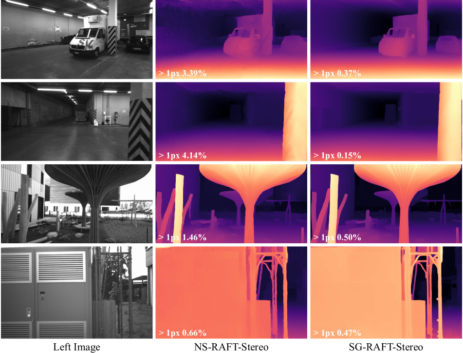
Figure 9: Visualization of ETH3D.

9 Comparison with StereoDiffusion

StereoDiffusion [37] introduces a training-free and straightforward method to generate stereo images using the original Stable Diffusion model without fine-tuning. We compare our method with StereoDiffusion under the same setup, utilizing the same left image and the corresponding pseudo disparity.

Although StereoDiffusion does not require additional training, in its mode of generating right images from left images, it relies on the null-text inversion technique to obtain the latent space representation of the left image, from which the corresponding right image is derived. This process needs to optimize the diffusion trajectory, resulting in a generation time of approximately 40 seconds per right image. In contrast, our model directly inpaints the mask, requiring only a few seconds to produce the right image, demonstrating a time efficiency improvement. Moreover, the null-text inversion technique does not perfectly reconstruct the left image, often introducing artifacts such as blurring, missing objects, or additional objects, which damage the original information. Additionally, StereoDiffusion performs the Stereo Pixel Shift operation in the latent space, leading to inconsistencies between the generated right image and the pseudo disparity.

As shown in Fig.  11, images generated by StereoDiffusion demonstrate these drawbacks. Warping in the latent space causes distortion, while null-text inversion causes missing objects, blurry backgrounds, and ghost artifacts. These images are difficult to use for stereo training.

Method	Cloudy		Foggy		Rainy		Sunny
	F	H	F	H	F	H	F	H
NS-RAFT-Stereo	8.81	2.95	18.18	3.41	29.19	8.47	7.42	2.88
SG-RAFT-Stereo	6.44	2.69	8.66	1.70	30.10	11.71	6.46	3.15

Table 7: Zero-shot generalization performance on DrivingStereo under different weather. We utilize >3px All in comparisons.

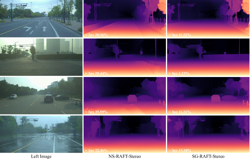
Figure 10: Visualization of DrivingStereo.

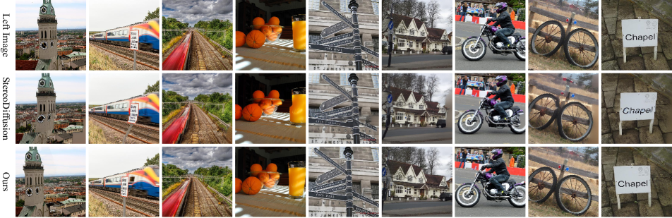
Figure 11: Visualization of StereoDiffusion and our diffusion inpainting model.

References

- Cabon et al. [2020] Yohann Cabon, Naila Murray, and Martin Humenberger. Virtual kitti 2. arXiv preprint arXiv:2001.10773, 2020.
- Chang and Chen [2018] Jia-Ren Chang and Yong-Sheng Chen. Pyramid stereo matching network. In Proceedings of the IEEE conference on computer vision and pattern recognition, pages 5410–5418, 2018.
- Chang et al. [2023] Tianyu Chang, Xun Yang, Tianzhu Zhang, and Meng Wang. Domain generalized stereo matching via hierarchical visual transformation. In Proceedings of the IEEE/CVF Conference on Computer Vision and Pattern Recognition, pages 9559–9568, 2023.
- Chen et al. [2016] Weifeng Chen, Zhao Fu, Dawei Yang, and Jia Deng. Single-image depth perception in the wild. Advances in neural information processing systems, 29, 2016.
- Chen et al. [2024] Ziyang Chen, Wei Long, He Yao, Yongjun Zhang, Bingshu Wang, Yongbin Qin, and Jia Wu. Mocha-stereo: Motif channel attention network for stereo matching. In Proceedings of the IEEE/CVF Conference on Computer Vision and Pattern Recognition, pages 27768–27777, 2024.
- Chuah et al. [2022] WeiQin Chuah, Ruwan Tennakoon, Reza Hoseinnezhad, Alireza Bab-Hadiashar, and David Suter. Itsa: An information-theoretic approach to automatic shortcut avoidance and domain generalization in stereo matching networks. In Proceedings of the IEEE/CVF Conference on Computer Vision and Pattern Recognition, pages 13022–13032, 2022.
- Guan et al. [2024] Tongfan Guan, Chen Wang, and Yun-Hui Liu. Neural markov random field for stereo matching. In Proceedings of the IEEE/CVF Conference on Computer Vision and Pattern Recognition, pages 5459–5469, 2024.
- Guo et al. [2022] Weiyu Guo, Zhaoshuo Li, Yongkui Yang, Zheng Wang, Russell H Taylor, Mathias Unberath, Alan Yuille, and Yingwei Li. Context-enhanced stereo transformer. In European Conference on Computer Vision, pages 263–279. Springer, 2022.
- Ho et al. [2020] Jonathan Ho, Ajay Jain, and Pieter Abbeel. Denoising diffusion probabilistic models. Advances in neural information processing systems, 33:6840–6851, 2020.
- Hornauer and Belagiannis [2022] Julia Hornauer and Vasileios Belagiannis. Gradient-based uncertainty for monocular depth estimation. In European Conference on Computer Vision, pages 613–630. Springer, 2022.
- Ke et al. [2024] Bingxin Ke, Anton Obukhov, Shengyu Huang, Nando Metzger, Rodrigo Caye Daudt, and Konrad Schindler. Repurposing diffusion-based image generators for monocular depth estimation. In Proceedings of the IEEE/CVF Conference on Computer Vision and Pattern Recognition, pages 9492–9502, 2024.
- Kendall et al. [2017] Alex Kendall, Hayk Martirosyan, Saumitro Dasgupta, Peter Henry, Ryan Kennedy, Abraham Bachrach, and Adam Bry. End-to-end learning of geometry and context for deep stereo regression. In Proceedings of the IEEE international conference on computer vision, pages 66–75, 2017.
- Kingma [2013] Diederik P Kingma. Auto-encoding variational bayes. arXiv preprint arXiv:1312.6114, 2013.
- Li et al. [2022] Jiankun Li, Peisen Wang, Pengfei Xiong, Tao Cai, Ziwei Yan, Lei Yang, Jiangyu Liu, Haoqiang Fan, and Shuaicheng Liu. Practical stereo matching via cascaded recurrent network with adaptive correlation. In Proceedings of the IEEE/CVF conference on computer vision and pattern recognition, pages 16263–16272, 2022.
- Li et al. [2021] Zhaoshuo Li, Xingtong Liu, Nathan Drenkow, Andy Ding, Francis X Creighton, Russell H Taylor, and Mathias Unberath. Revisiting stereo depth estimation from a sequence-to-sequence perspective with transformers. In Proceedings of the IEEE/CVF international conference on computer vision, pages 6197–6206, 2021.
- Lin et al. [2014] Tsung-Yi Lin, Michael Maire, Serge Belongie, James Hays, Pietro Perona, Deva Ramanan, Piotr Dollár, and C Lawrence Zitnick. Microsoft coco: Common objects in context. In Computer Vision–ECCV 2014: 13th European Conference, Zurich, Switzerland, September 6-12, 2014, Proceedings, Part V 13, pages 740–755. Springer, 2014.
- Lipson et al. [2021] Lahav Lipson, Zachary Teed, and Jia Deng. Raft-stereo: Multilevel recurrent field transforms for stereo matching. In 2021 International Conference on 3D Vision (3DV), pages 218–227. IEEE, 2021.
- Liu et al. [2022] Biyang Liu, Huimin Yu, and Guodong Qi. Graftnet: Towards domain generalized stereo matching with a broad-spectrum and task-oriented feature. In Proceedings of the IEEE/CVF conference on computer vision and pattern recognition, pages 13012–13021, 2022.
- Lugmayr et al. [2022] Andreas Lugmayr, Martin Danelljan, Andres Romero, Fisher Yu, Radu Timofte, and Luc Van Gool. Repaint: Inpainting using denoising diffusion probabilistic models. In Proceedings of the IEEE/CVF conference on computer vision and pattern recognition, pages 11461–11471, 2022.
- Luo et al. [2018] Yue Luo, Jimmy Ren, Mude Lin, Jiahao Pang, Wenxiu Sun, Hongsheng Li, and Liang Lin. Single view stereo matching. In Proceedings of the IEEE conference on computer vision and pattern recognition, pages 155–163, 2018.
- Mayer et al. [2016] Nikolaus Mayer, Eddy Ilg, Philip Hausser, Philipp Fischer, Daniel Cremers, Alexey Dosovitskiy, and Thomas Brox. A large dataset to train convolutional networks for disparity, optical flow, and scene flow estimation. In Proceedings of the IEEE conference on computer vision and pattern recognition, pages 4040–4048, 2016.
- Menze and Geiger [2015] Moritz Menze and Andreas Geiger. Object scene flow for autonomous vehicles. In Proceedings of the IEEE conference on computer vision and pattern recognition, pages 3061–3070, 2015.
- Mildenhall et al. [2021] Ben Mildenhall, Pratul P Srinivasan, Matthew Tancik, Jonathan T Barron, Ravi Ramamoorthi, and Ren Ng. Nerf: Representing scenes as neural radiance fields for view synthesis. Communications of the ACM, 65(1):99–106, 2021.
- Neuhold et al. [2017] Gerhard Neuhold, Tobias Ollmann, Samuel Rota Bulo, and Peter Kontschieder. The mapillary vistas dataset for semantic understanding of street scenes. In Proceedings of the IEEE international conference on computer vision, pages 4990–4999, 2017.
- Pumarola et al. [2021] Albert Pumarola, Enric Corona, Gerard Pons-Moll, and Francesc Moreno-Noguer. D-nerf: Neural radiance fields for dynamic scenes. In Proceedings of the IEEE/CVF Conference on Computer Vision and Pattern Recognition, pages 10318–10327, 2021.
- Rao et al. [2023] Zhibo Rao, Bangshu Xiong, Mingyi He, Yuchao Dai, Renjie He, Zhelun Shen, and Xing Li. Masked representation learning for domain generalized stereo matching. In Proceedings of the IEEE/CVF Conference on Computer Vision and Pattern Recognition, pages 5435–5444, 2023.
- Rombach et al. [2022] Robin Rombach, Andreas Blattmann, Dominik Lorenz, Patrick Esser, and Björn Ommer. High-resolution image synthesis with latent diffusion models. In Proceedings of the IEEE/CVF conference on computer vision and pattern recognition, pages 10684–10695, 2022.
- Scharstein et al. [2014] Daniel Scharstein, Heiko Hirschmüller, York Kitajima, Greg Krathwohl, Nera Nešić, Xi Wang, and Porter Westling. High-resolution stereo datasets with subpixel-accurate ground truth. In Pattern Recognition: 36th German Conference, GCPR 2014, Münster, Germany, September 2-5, 2014, Proceedings 36, pages 31–42. Springer, 2014.
- Schops et al. [2017] Thomas Schops, Johannes L Schonberger, Silvano Galliani, Torsten Sattler, Konrad Schindler, Marc Pollefeys, and Andreas Geiger. A multi-view stereo benchmark with high-resolution images and multi-camera videos. In Proceedings of the IEEE conference on computer vision and pattern recognition, pages 3260–3269, 2017.
- Shen et al. [2021] Zhelun Shen, Yuchao Dai, and Zhibo Rao. Cfnet: Cascade and fused cost volume for robust stereo matching. In Proceedings of the IEEE/CVF conference on computer vision and pattern recognition, pages 13906–13915, 2021.
- Song et al. [2020] Jiaming Song, Chenlin Meng, and Stefano Ermon. Denoising diffusion implicit models. arXiv preprint arXiv:2010.02502, 2020.
- Teed and Deng [2020] Zachary Teed and Jia Deng. Raft: Recurrent all-pairs field transforms for optical flow. In Computer Vision–ECCV 2020: 16th European Conference, Glasgow, UK, August 23–28, 2020, Proceedings, Part II 16, pages 402–419. Springer, 2020.
- Tonioni et al. [2019a] Alessio Tonioni, Oscar Rahnama, Thomas Joy, Luigi Di Stefano, Thalaiyasingam Ajanthan, and Philip HS Torr. Learning to adapt for stereo. In Proceedings of the IEEE/CVF Conference on Computer Vision and Pattern Recognition, pages 9661–9670, 2019a.
- Tonioni et al. [2019b] Alessio Tonioni, Fabio Tosi, Matteo Poggi, Stefano Mattoccia, and Luigi Di Stefano. Real-time self-adaptive deep stereo. In Proceedings of the IEEE/CVF conference on computer vision and pattern recognition, pages 195–204, 2019b.
- Tosi et al. [2023] Fabio Tosi, Alessio Tonioni, Daniele De Gregorio, and Matteo Poggi. Nerf-supervised deep stereo. In Proceedings of the IEEE/CVF conference on computer vision and pattern recognition, pages 855–866, 2023.
- Vasiljevic et al. [2019] Igor Vasiljevic, Nick Kolkin, Shanyi Zhang, Ruotian Luo, Haochen Wang, Falcon Z Dai, Andrea F Daniele, Mohammadreza Mostajabi, Steven Basart, Matthew R Walter, et al. Diode: A dense indoor and outdoor depth dataset. arXiv preprint arXiv:1908.00463, 2019.
- Wang et al. [2024a] Lezhong Wang, Jeppe Revall Frisvad, Mark Bo Jensen, and Siavash Arjomand Bigdeli. Stereodiffusion: Training-free stereo image generation using latent diffusion models. In Proceedings of the IEEE/CVF Conference on Computer Vision and Pattern Recognition, pages 7416–7425, 2024a.
- Wang et al. [2020] Wenshan Wang, Delong Zhu, Xiangwei Wang, Yaoyu Hu, Yuheng Qiu, Chen Wang, Yafei Hu, Ashish Kapoor, and Sebastian Scherer. Tartanair: A dataset to push the limits of visual slam. In 2020 IEEE/RSJ International Conference on Intelligent Robots and Systems (IROS), pages 4909–4916. IEEE, 2020.
- Wang et al. [2024b] Xianqi Wang, Gangwei Xu, Hao Jia, and Xin Yang. Selective-stereo: Adaptive frequency information selection for stereo matching. In Proceedings of the IEEE/CVF Conference on Computer Vision and Pattern Recognition, pages 19701–19710, 2024b.
- Watson et al. [2020] Jamie Watson, Oisin Mac Aodha, Daniyar Turmukhambetov, Gabriel J Brostow, and Michael Firman. Learning stereo from single images. In Computer Vision–ECCV 2020: 16th European Conference, Glasgow, UK, August 23–28, 2020, Proceedings, Part I 16, pages 722–740. Springer, 2020.
- Xiang et al. [2024] Mochu Xiang, Jing Zhang, Nick Barnes, and Yuchao Dai. Measuring and modeling uncertainty degree for monocular depth estimation. IEEE Transactions on Circuits and Systems for Video Technology, 2024.
- Xu et al. [2022] Gangwei Xu, Junda Cheng, Peng Guo, and Xin Yang. Attention concatenation volume for accurate and efficient stereo matching. In Proceedings of the IEEE/CVF Conference on Computer Vision and Pattern Recognition, pages 12981–12990, 2022.
- Xu et al. [2023] Gangwei Xu, Xianqi Wang, Xiaohuan Ding, and Xin Yang. Iterative geometry encoding volume for stereo matching. In Proceedings of the IEEE/CVF Conference on Computer Vision and Pattern Recognition, pages 21919–21928, 2023.
- Xu et al. [2024] Gangwei Xu, Xianqi Wang, Zhaoxing Zhang, Junda Cheng, Chunyuan Liao, and Xin Yang. Igev++: Iterative multi-range geometry encoding volumes for stereo matching. arXiv preprint arXiv:2409.00638, 2024.
- Yang et al. [2024] Lihe Yang, Bingyi Kang, Zilong Huang, Zhen Zhao, Xiaogang Xu, Jiashi Feng, and Hengshuang Zhao. Depth anything v2. arXiv preprint arXiv:2406.09414, 2024.
- Zhang et al. [2020] Feihu Zhang, Xiaojuan Qi, Ruigang Yang, Victor Prisacariu, Benjamin Wah, and Philip Torr. Domain-invariant stereo matching networks. In Computer Vision–ECCV 2020: 16th European Conference, Glasgow, UK, August 23–28, 2020, Proceedings, Part II 16, pages 420–439. Springer, 2020.
- Zhang et al. [2023] Lvmin Zhang, Anyi Rao, and Maneesh Agrawala. Adding conditional control to text-to-image diffusion models. In Proceedings of the IEEE/CVF International Conference on Computer Vision, pages 3836–3847, 2023.
- Zhou et al. [2017] Bolei Zhou, Hang Zhao, Xavier Puig, Sanja Fidler, Adela Barriuso, and Antonio Torralba. Scene parsing through ade20k dataset. In Proceedings of the IEEE conference on computer vision and pattern recognition, pages 633–641, 2017.