Geometry of Sparsity-Inducing Norms

Abstract

Sparse optimization seeks an optimal solution with few nonzero entries. To achieve this, it is common to add to the criterion a penalty term proportional to the $\ell_{1}$-norm, which is recognized as the archetype of sparsity-inducing norms. In this approach, the number of nonzero entries is not controlled a priori. By contrast, in this paper, we focus on finding an optimal solution with at most $k$ nonzero coordinates (or for short, $k$-sparse vectors), where $k$ is a given sparsity level (or “sparsity budget”). For this purpose, we study the class of generalized $k$-support norms that arise from a given source norm. When added as a penalty term, we provide conditions under which such generalized $k$-support norms promote $k$-sparse solutions. The result follows from an analysis of the exposed faces of closed convex sets generated by $k$-sparse vectors, and of how primal support identification can be deduced from dual information. Finally, we study some of the geometric properties of the unit balls for the $k$-support norms and their dual norms when the source norm belongs to the family of $\ell_{p}$-norms.

Keywords: sparsity, $\ell_{0}$ pseudonorm, orthant-monotonicity, top-$k$ norm, $k$-support norm

2020 Mathematics Subject Classification (MSC2020): 49N15 90C25 52A05 52A21

1 Introduction

In 1996, Tibshirani [27] proposed least-square regression with an $\ell_{1}$-norm penalty to achieve sparsity in least-square optimization. Figure 1 is the replica of [27, Figure 2], which provides insight regarding why corresponding optimal solutions are sparse (we copy the comments of [27, Figure 2] with additional precisions in brackets [$\cdots$]):

“The elliptical contours of this function [quadratic criterion] are shown by the full curves in Fig. 2(a); they are centred at the OLS [optimal least-square] estimates; the constraint region [$\ell_{1}$-ball in dimension 2] is the rotated square. The lasso solution is the first place that the contours touch the square, and this will sometimes occur at a corner, corresponding to a zero coefficient. The picture for ridge regression is shown in Fig. 2(b): there are no corners for the contours to hit and hence zero solutions will rarely result.”

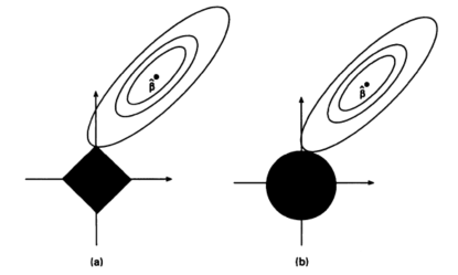
Figure 1: Replica of [27, Figure 2]

Thus, as the kinks of the $\ell_{1}$-ball are located at sparse points, it is common to say that the $\ell_{1}$-norm is sparsity-inducing. Figure 2 shows two examples of unit balls with kinks located at sparse points. Both of them arise from norms that are studied in the sequel.

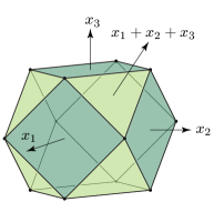
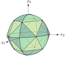
Figure 2: Two examples of unit balls with kinks located at sparse points

A natural question that arises from the comments of [27, Figure 2] is: What could be mathematical conditions for inducing sparsity?

Going beyond least-square regression with an $\ell_{1}$-norm penalty, one can consider optimization problems of the form $\min_{x\in{\mathbb{R}}^{d}}\big{(}{f({x})+\gamma\lvert\hskip-1.19995pt\lvert{x}\rvert\hskip-1.19995pt\rvert}\big{)}$, where $f:{\mathbb{R}}^{d}\to{\mathbb{R}}$ is a smooth convex function, $\gamma>0$ and $\lvert\hskip-1.19995pt\lvert{\cdot}\rvert\hskip-1.19995pt\rvert$ is a norm with unit ball $B$. This is the approach taken in the papers [2, 18], where the terminology “sparsity-inducing norm” has been introduced. As all functions take finite values — and as $\lvert\hskip-1.19995pt\lvert{\cdot}\rvert\hskip-1.19995pt\rvert$ is the support function $\sigma_{{B}^{\odot}}$ of the polar set ${B}^{\odot}$ — a solution $x^{\sharp}$ of the above problem is characterized by the Fermat rule

$$0\in\nabla f({x^{\sharp}})+\gamma\partial\sigma_{{B}^{\odot}}({x^{\sharp}})\;,$$

where $\partial\sigma_{{B}^{\odot}}({x^{\sharp}})$ is the face $F_{\bot}({B}^{\odot},x^{\sharp})$ of ${B}^{\odot}$ exposed by $x^{\sharp}$. Thus, the optimality condition reads

$$-\nabla f({x^{\sharp}})\in\gamma F_{\bot}({B}^{\odot},x^{\sharp})$$

and, by polarity [11, Theorem 5.1], this is equivalent to

$$\frac{x^{\sharp}}{\lvert\hskip-1.19995pt\lvert{x^{\sharp}}\rvert\hskip-1.19995pt\rvert}\in F_{\bot}(B,-\nabla f({x^{\sharp}}))\;.$$

One could say that the considered norm is sparsity-inducing if information about the support of $x^{\sharp}$ could be obtained from information about the exposed faces $F_{\bot}(B,-\nabla f({x^{\sharp}}))$ of the unit ball $B$ for that norm. This is the approach that we consider in this paper. More precisely, we analyze the exposed faces of some special convex sets, and in particular of the unit balls of certain norms, and relate them to sparsity.

Our work is related to different trends in the literature. As said above, the terminology “sparsity-inducing norm” has been introduced in the papers [2, 18], which focus on algorithmic issues, whereas we focus on geometric aspects. In particular, we study how the gradient — at a solution, of the original smooth function to be minimized — provides relevant (dual) information about the sparsity of the (primal) solution. Sparsity is also examined for the solutions of undetermined linear systems, and we emphasize the three papers [5, 8, 4]. The paper [5] studies the solutions of an undetermined linear system in the context of compressed sensing; it provides a sufficient property of the sensing matrix, the restricted isometry property, which ensures that the minimal $\ell_{1}$-norm solution coincides with the sparse solution. In [8], it is explained how to design so-called “atomic norms” which promote sparsity, but with respect to a given (compact) atomic set. [8] stresses that it is “the favorable facial structure of the atomic norm ball that makes the atomic norm a suitable convex heuristic to recover simple models”. The norms that we present in Sect. 3 are atomic norms where the atomic set is especially designed to provide solutions with an a priori given “sparsity budget” (number of nonzero entries bounded above by a given integer); we focus on the geometric description of the facial structure of the unit balls of these special atomic norms. As said above, we study in particular how a gradient provides relevant (dual) information about sparsity of the (primal) solution. By contrast, [8] focuses more on measuring the Gaussian width of the tangent cones as a way to to achieve more or less sparsity. The paper [4] also stresses the role of faces in identifying solutions of undetermined linear systems that can be expressed as convex combinations of a small number of atoms. Where [4] studies faces, we focus on exposed faces and on how dual information is related to sparsity of a primal solution. Let us mention three more works. The question of decomposing a vector as a convex conical combination of elementary atoms has been studied in [11], with a special role given to the so-called alignment, that is, to normal cones and exposed faces. Our approach intersects that of [11], but with a focus on the classic sparsity along coordinate axis and with the goal to describe the geometry of some unit balls [7]. In [10], the focus is put on stratifying the primal space. Then, an optimal primal-dual pair $({x^{\sharp},\nabla f({x^{\sharp}})})$ can provide information on the strata to which $x^{\sharp}$ belongs. General regularizers (and not only norms) are studied. Convex structured sparsity with norms is the object of [22], but there is no focus on how normal cones and exposed faces relate to sparsity.

To summarize, to the difference with the literature mentioned above, we focus on sparsity-inducing norms that promote solutions within an a priori “sparsity budget” by using dual information.

The paper is organized as follows. In Sect. 2, after providing background on sparsity and on faces of closed convex sets, we state our main result: we characterize the faces of closed convex sets whose extreme points are $k$-sparse, from which we deduce support identification. In Sect. 3, we characterize the faces of the unit ball of $k$-support norms, from which we deduce support identification. Then, we provide dual conditions under which the primal optimal solution of a minimization problem, penalized by a $k$-support norm, is $k$-sparse. In the cases of orthant-monotonic and orthant-strictly monotonic source norms, we obtain a characterization of the intersection of the $k$-sparse vectors with the faces of the $k$-support norm. Sect. 4 deals with the geometric aspects of the face and cone lattices of the unit balls of top-($q$,$k$) norm and ($p$,$k$)-support norms, that is, with the $\ell_{p}$ as source norms.

2 Face characterization and support identification

In §2.1, we provide background on sparsity and on faces of closed convex sets. In §2.2, we state our main result: we characterize the faces of closed convex sets whose extreme points are $k$-sparse, from which we deduce support identification. Proofs are given in §2.3.

2.1 Background on sparsity and on faces of closed convex sets

We consider the finite-dimensional real Euclidean vector space ${\mathbb{R}}^{d}$ equipped with the scalar product $\left\langle\,\mid\>\right\rangle$.

Background on sparsity

We use the notation $\llbracket j,k\rrbracket=\{{j,j+1,\ldots,k-1,k}\}$ for any pair of integers such that $j\leq k$. Let ${d}$ be a natural number. Denoting by ${\lvert K\rvert}$ the cardinality of a subset $K\subset\llbracket 1,{d}\rrbracket$, we define, for any vector $x$ in ${\mathbb{R}}^{d}$, the support of $x$ by

$$\mathrm{supp}({x}) =\big{\{}{j\in\llbracket 1,{d}\rrbracket:\,x_{j}\not=0}\big{\}}\subset\llbracket 1,{d}\rrbracket\;,\enspace$$ (1a)

and the $$\ell_{0} x$$ pseudonorm of  by the number of nonzero components, that is, by

$$\ell_{0}({x}) ={\lvert\mathrm{supp}({x})\rvert}\;.$$ (1b)

This defines the $\ell_{0}$ pseudonorm function $\ell_{0}:{\mathbb{R}}^{d}\to\llbracket 0,{d}\rrbracket$. For any $k$ in $\llbracket 1,{d}\rrbracket$, we denote its level sets, made of all the vectors with at most $k$ nonzero coordinates by

$$\ell_{0}^{\leq k}=\{{x\in{\mathbb{R}}^{d}:\,\ell_{0}({x})\leq k}\}$$ (2a)

The vectors in $\ell_{0}^{\leq k}$ will be called $k$-sparse vectors. For any subset $K$ of $\llbracket 1,{d}\rrbracket$, we introduce the subspace ${\cal R}_{K}$ of ${\mathbb{R}}^{d}$ made of vectors whose components vanish outside of $K$ as

$${\cal R}_{K}=\big{\{}{x\in{\mathbb{R}}^{d}:\,x_{j}=0\;,\enspace\forall j\not\in K}\big{\}}$$ (2b)

with the convention that ${\cal R}_{\emptyset}=\{{0}\}$. Using $\bigcup_{{\lvert K\rvert}\leq k}$ as a shorthand for $\bigcup_{K\subset\llbracket 1,{d}\rrbracket,{\lvert K\rvert}\leq k}$, we get

$${\ell_{0}^{\leq k}}=\bigcup_{{\lvert K\rvert}\leq k}{\cal R}_{K}\;.$$ (2c)

We denote by $\pi_{K}:{\mathbb{R}}^{d}\to{\cal R}_{K}$ the orthogonal projection mapping; for any vector $x$ in ${\mathbb{R}}^{d}$, the coordinates of the vector $\pi_{K}x\in{\cal R}_{K}$ coincide with those of $x$, except for the ones whose indices range outside of $K$ that are equal to zero. It is easily seen that the orthogonal projection mapping $\pi_{K}$ is self-adjoint (or self-dual), that is,

$$\left\langle\pi_{K}x\mid\>y\right\rangle=\left\langle x\mid\>\pi_{K}y\right\rangle=\left\langle\pi_{K}x\mid\>\pi_{K}y\right\rangle\;,\enspace\forall x\in{\mathbb{R}}^{d}\;,\enspace\forall y\in{\mathbb{R}}^{d}\;.$$ (3)

Background on faces of closed convex sets

For any subset $X\subset{\mathbb{R}}^{d}$, the expression

$$\sigma_{X}({y})=\sup_{x\in X}\left\langle x\mid\>y\right\rangle\;,\enspace\forall y\in{\mathbb{R}}^{d}$$ (4)

defines a map $\sigma_{X}:{\mathbb{R}}^{d}\to\overline{\mathbb{R}}$ called the support function of the subset $X$. The (negative) polar set ${X}^{\odot}$ of the subset $X\subset{\mathbb{R}}^{d}$ is the closed convex set

$${X}^{\odot}=\big{\{}{y\in{\mathbb{R}}^{d}:\,\langle{x,\,y}\rangle\leq 1\;,\enspace\forall x\in X}\big{\}}=\{{\sigma_{X}\leq 1}\}\;.$$ (5)

The face of a nonempty closed convex subset $C$ of ${\mathbb{R}}^{d}$ exposed by a dual vector $y$ in ${\mathbb{R}}^{d}$ is

$$F_{\bot}(C,y)=\mathop{\arg\max}_{x\in C}\left\langle x\mid\>y\right\rangle\;,$$ (6)

and the normal cone $N(C,x)$ of $C$ at a primal vector $x\in C$ is defined by the conjugacy relation

$$x\in C\,\mbox{ and }\,y\in N(C,x)\iff x\in F_{\bot}(C,y)\;.$$ (7)

2.2 Convex sets with $k$-sparse extreme points

As discussed in the introduction, the intuition behind [27, Figure 2] is that the unit ball of a sparsity-inducing norm should have extreme points (vertices) precisely at $k$-sparse vectors. One way to enforce this is to select a suitable subset of $k$-sparse vectors, and then take the convex closure. Theorem 1 characterizes the faces of this convex closure.

Theorem 1 (Characterization of faces)

Let $k\in\llbracket 1,{d}\rrbracket$ be a natural number and $X\subset{\mathbb{R}}^{d}$ be a (primal) nonempty set. We set

$$X_{k}=\bigcup_{{\lvert K\rvert}\leq k}\pi_{K}({X})\;.$$ (8)

Let $y\in{\mathbb{R}}^{d}$ be a (dual) vector. We set

$${\mathcal{K}}^{\sharp}_{X,k}({y})=\mathop{\arg\max}_{\begin{subarray}{c}K\subset\llbracket 1,{d}\rrbracket\\ {\lvert K\rvert}\leq k\end{subarray}}\sigma_{\overline{\mathrm{co}}X}({\pi_{K}y})\;,$$ (9)

which is such that $\emptyset\neq{\mathcal{K}}^{\sharp}_{X,k}({y})\subset\big{\{}{K\subset\llbracket 1,{d}\rrbracket,{\lvert K\rvert}\leq k}\big{\}}\subset 2^{\llbracket 1,{d}\rrbracket}$. Then, we have that the set $X_{k}$ is made of $k$-sparse vectors, that is,

$$X_{k}\subset{\ell_{0}^{\leq k}}\;,$$ (10)

and the faces of $\overline{\mathrm{co}}X_{k}$ are related to the faces of $\overline{\mathrm{co}}X$ by

$$X_{k}\cap F_{\bot}\big{(}{\overline{\mathrm{co}}X_{k},y}\big{)}=\Big{\{}{\pi_{K^{\sharp}}\big{(}{X\cap F_{\bot}(\overline{\mathrm{co}}X,\pi_{K^{\sharp}}y)}\big{)}:\,K^{\sharp}\in{\mathcal{K}}^{\sharp}_{X,k}({y})}\Big{\}}\;,$$ (11)

and by

$$F_{\bot}\big{(}{\overline{\mathrm{co}}X_{k},y}\big{)}=\overline{\mathrm{co}}\Big{\{}{\pi_{K^{\sharp}}\big{(}{X\cap F_{\bot}(\overline{\mathrm{co}}X,\pi_{K^{\sharp}}y)}\big{)}:\,K^{\sharp}\in{\mathcal{K}}^{\sharp}_{X,k}({y})}\Big{\}}\;.$$ (12)

By construction, the extreme points of $\overline{\mathrm{co}}X_{k}$ are contained in $X_{k}$, while $X_{k}$ itself is a subset of $\bigcup_{{\lvert K\rvert}\leq k}{\cal R}_{K}={\ell_{0}^{\leq k}}$ (see Equation (10)), hence is made of $k$-sparse vectors.

Corollary 2 (Support identification)

Under the assumptions of Theorem 1,

$$x\in X_{k}\cap F_{\bot}(\overline{\mathrm{co}}X_{k},y) \implies\mathrm{supp}({x})\in{\mathcal{K}}^{\sharp}_{X,k}({y})\;,$$ (13)

$$x\in F_{\bot}(\overline{\mathrm{co}}X_{k},y) \implies\mathrm{supp}({x})\subset\bigcup_{K^{\sharp}\in{\mathcal{K}}^{\sharp}_{X,k}({y})}K^{\sharp}\;.$$ (14)

2.3 Proofs of Theorem 1 and Corollary 2

We begin the section by proving the following preparatory lemma.

Lemma 3

Consider a (primal) nonempty subset $X$ of ${\mathbb{R}}^{d}$. For any (dual) vector $y$ contained in ${\mathbb{R}}^{d}$ and any subset $K$ of $\llbracket 1,{d}\rrbracket$, we have that

$$\mathop{\arg\max}_{x\in\pi_{K}({X})}\langle{x\,|\,\,y}\rangle=\pi_{K}\Big{(}{\mathop{\arg\max}_{z\in X}\langle{z\,|\,\,\pi_{K}y}\rangle}\Big{)}$$ (15)

and that

$$\max_{x\in\pi_{K}({X})}\langle{x\,|\,\,y}\rangle=\sigma_{\overline{\mathrm{co}}X}({\pi_{K}y})\;.$$ (16)

Proof. We prove (15) by establishing two opposite inclusions. On the one hand, the inclusion

$$\mathop{\arg\max}_{x\in\pi_{K}({X})}\langle{x\,|\,\,y}\rangle\subset\pi_{K}\Big{(}{\mathop{\arg\max}_{z\in X}\langle{z\,|\,\,\pi_{K}y}\rangle}\Big{)}$$

holds true as a consequence of the following sequence of equivalences and implications:

$$x^{\sharp}\in\mathop{\arg\max}_{x\in\pi_{K}({X})}\langle{x\,|\,\,y}\rangle\iff x^{\sharp}\in\pi_{K}({X})\,\mbox{ and }\,\langle{x^{\sharp}\,|\,\,y}\rangle\geq\langle{x\,|\,\,y}\rangle\;,\enspace\forall x\in\pi_{K}({X})$$

$$\iff x^{\sharp}\in\pi_{K}({X})\,\mbox{ and }\,\langle{x^{\sharp}\,|\,\,y}\rangle\geq\langle{\pi_{K}z\,|\,\,y}\rangle\;,\enspace\forall z\in X \pi_{K}({X})$$ (by definition of )

$$\implies x^{\sharp}\in\pi_{K}({X})\,\mbox{ and }\,\langle{\pi_{K}x^{\sharp}\,|\,\,y}\rangle\geq\langle{\pi_{K}z\,|\,\,y}\rangle\;,\enspace\forall z\in X$$

because $$x^{\sharp}\in\pi_{K}({X}) \pi_{K} x^{\sharp}=\pi_{K}x^{\sharp}$$ belongs to the image of the orthogonal projection , hence ,

$$\implies x^{\sharp}\in\pi_{K}({X})\,\mbox{ and }\,\langle{x^{\sharp}\,|\,\,\pi_{K}y}\rangle\geq\langle{z\,|\,\,\pi_{K}y}\rangle\;,\enspace\forall z\in X \pi_{K}$$ (as the orthogonal projection  is self-adjoint, see (3))

$$\implies x^{\sharp}\in\pi_{K}({X})\,\mbox{ and }\,x^{\sharp}\in\mathop{\arg\max}_{z\in X}\langle{z\,|\,\,\pi_{K}y}\rangle$$

$$\implies x^{\sharp}\in\pi_{K}({X})\,\mbox{ and }\,\pi_{K}x^{\sharp}\in\pi_{K}\Big{(}{\mathop{\arg\max}_{z\in X}\langle{z\,|\,\,\pi_{K}y}\rangle}\Big{)}$$

$$\implies x^{\sharp}\in\pi_{K}({X})\,\mbox{ and }\,x^{\sharp}\in\pi_{K}\Big{(}{\mathop{\arg\max}_{z\in X}\langle{z\,|\,\,\pi_{K}y}\rangle}\Big{)} x^{\sharp}=\pi_{K}x^{\sharp}$$ (as .)

On the other hand, the inclusion

$$\pi_{K}\Big{(}{\mathop{\arg\max}_{z\in X}\langle{z\,|\,\,\pi_{K}y}\rangle}\Big{)}\subset\mathop{\arg\max}_{x\in\pi_{K}({X})}\langle{x\,|\,\,y}\rangle$$

holds true as a consequence of the following equivalences and implications:

$$x^{\sharp}\in\pi_{K}\Big{(}{\mathop{\arg\max}_{z\in X}\langle{z\,|\,\,\pi_{K}y}\rangle}\Big{)}\iff \exists z^{\sharp}\in\mathop{\arg\max}_{z\in X}\langle{z\,|\,\,\pi_{K}y}\rangle\text{ and }x^{\sharp}=\pi_{K}z^{\sharp}$$

$$\iff x^{\sharp}=\pi_{K}z^{\sharp}\text{ where }z^{\sharp}\in X\text{ and }\langle{z^{\sharp}\,|\,\,\pi_{K}y}\rangle\geq\langle{z\,|\,\,\pi_{K}y}\rangle\;,\enspace\forall z\in X$$

$$\iff x^{\sharp}=\pi_{K}z^{\sharp}\text{ where }z^{\sharp}\in X\text{ and }\langle{\pi_{K}z^{\sharp}\,|\,\,y}\rangle\geq\langle{\pi_{K}z\,|\,\,y}\rangle\;,\enspace\forall z\in X \pi_{K}$$ (as the orthogonal projection  is self-adjoint, see (3))

$$\implies x^{\sharp}\in\pi_{K}({X})\text{ and }\langle{x^{\sharp}\,|\,\,y}\rangle\geq\langle{x\,|\,\,y}\rangle\;,\enspace\forall x\in\pi_{K}({X})$$

$$\implies x^{\sharp}=\pi_{K}x^{\sharp}\in\pi_{K}({X})\text{ and }\langle{x^{\sharp}\,|\,\,y}\rangle\geq\langle{x\,|\,\,y}\rangle\;,\enspace\forall x\in\pi_{K}({X})$$

because $$x^{\sharp}\in\pi_{K}({X}) \pi_{K} x^{\sharp}=\pi_{K}x^{\sharp}$$ belongs to the image of the orthogonal projection , hence ,

$$\implies x^{\sharp}\in\mathop{\arg\max}_{x\in\pi_{K}({X})}\langle{x\,|\,\,y}\rangle \mathop{\arg\max}_{x\in\pi_{K}({X})}\langle{x\,|\,\,y}\rangle$$ (by definition of .)

Finally (16) holds true because, as the orthogonal projection $\pi_{K}$ is self-adjoint (see (3)),

$$\max_{x\in\pi_{K}({X})}\langle{x\,|\,\,y}\rangle=\max_{z\in X}\langle{\pi_{K}z\,|\,\,y}\rangle=\max_{z\in X}\langle{z\,|\,\,\pi_{K}y}\rangle=\sigma_{\overline{\mathrm{co}}X}({\pi_{K}y})\;,$$

by definition (4) and the well-known property $\sigma_{X}=\sigma_{\overline{\mathrm{co}}X}$ of the support function $\sigma_{X}$. $\Box$

2.3.1 Proof of Theorem 1

Proof. Consider a number $k$ in $\llbracket 1,{d}\rrbracket$, a (primal) nonempty subset $X$ of ${\mathbb{R}}^{d}$, and a (dual) vector $y$ in ${\mathbb{R}}^{d}$. First observe that

$$\emptyset\neq{\mathcal{K}}^{\sharp}_{X,k}({y})\subset\big{\{}{K\subset\llbracket 1,{d}\rrbracket,{\lvert K\rvert}\leq k}\big{\}}\subset 2^{\llbracket 1,{d}\rrbracket}.$$

Second, Equation (10) follows from the definition (8) of $X_{k}$ as by (2c),

$$X_{k}=\bigcup_{{\lvert K\rvert}\leq k}\pi_{K}({X})\subset\bigcup_{{\lvert K\rvert}\leq k}{\cal R}_{K}={\ell_{0}^{\leq k}}$$

Third, we prove (11). We have that

$$x^{\sharp}\in{X_{k}}\cap F_{\bot}(\overline{\mathrm{co}}{X_{k}},y) \iff x^{\sharp}\in\mathop{\arg\max}_{x\in X_{k}}\langle{x\,|\,\,y}\rangle$$

as $$F_{\bot}(\overline{\mathrm{co}}{X_{k}},y)=\mathop{\arg\max}_{x\in\overline{\mathrm{co}}{X_{k}}}\langle{x\,|\,\,y}\rangle \max_{x\in X_{k}}\left\langle x\mid\>y\right\rangle=\max_{x\in\overline{\mathrm{co}}{X_{k}}}\left\langle x\mid\>y\right\rangle$$ and ,

$$\iff x^{\sharp}\in{X_{k}}\text{ and }\langle{x^{\sharp}\,|\,\,y}\rangle=\max_{x\in\bigcup_{{\lvert K\rvert}\leq k}\pi_{K}({X})}\langle{x\,|\,\,y}\rangle$$

using the definition (8) of $$X_{k} {\lvert K\rvert}\leq k K\subset\llbracket 1,{d}\rrbracket,{\lvert K\rvert}\leq k$$ and where, in all this proof, the subscript has to be understood as ,

$$\iff x^{\sharp}\in{X_{k}}\text{ and }\langle{x^{\sharp}\,|\,\,y}\rangle=\max_{{\lvert K\rvert}\leq k}\max_{x\in\pi_{K}({X})}\langle{x\,|\,\,y}\rangle$$

$$\iff x^{\sharp}\in{X_{k}}\text{ and there exists }K^{\sharp}\subset\llbracket 1,{d}\rrbracket\;,\enspace{\lvert K^{\sharp}\rvert}\leq k\text{ such that}$$

$$\hphantom{\iff\text{ }}x^{\sharp}\in\pi_{K^{\sharp}}({X})\text{ and }\langle{x^{\sharp}\,|\,\,y}\rangle=\max_{{\lvert K\rvert}\leq k}\max_{x\in\pi_{K}({X})}\langle{x\,|\,\,y}\rangle$$

because, by definition (8) of $$X_{k} x^{\sharp}\in\bigcup_{{\lvert K\rvert}\leq k}\pi_{K}({X}) K^{\sharp}\subset\llbracket 1,{d}\rrbracket {\lvert K^{\sharp}\rvert}\leq k x^{\sharp}\in\pi_{K^{\sharp}}({X})$$, , hence there exists with such that ,

$$\iff x^{\sharp}\in{X_{k}}\text{ and there exists }K^{\sharp}\subset\llbracket 1,{d}\rrbracket\;,\enspace{\lvert K^{\sharp}\rvert}\leq k\text{ such that}$$

$$\hphantom{\iff\text{ }}x^{\sharp}\in\pi_{K^{\sharp}}({X})\text{ and }\langle{x^{\sharp}\,|\,\,y}\rangle=\max_{{\lvert K\rvert}\leq k}\max_{x\in\pi_{K}({X})}\langle{x\,|\,\,y}\rangle$$

$$\hphantom{\iff\text{ }}\text{ and }K^{\sharp}\in\mathop{\arg\max}_{{\lvert K\rvert}\leq k}\max_{x\in\pi_{K}({X})}\langle{x\,|\,\,y}\rangle \mathop{\arg\max}_{{\lvert K\rvert}\leq k}\max_{x\in\pi_{K}({X})}\langle{x\,|\,\,y}\rangle$$ (by definition of )

$$\iff x^{\sharp}\in{X_{k}}\text{ and there exists }K^{\sharp}\in\mathop{\arg\max}_{{\lvert K\rvert}\leq k}\max_{x\in\pi_{K}({X})}\langle{x\,|\,\,y}\rangle\text{ such that}$$

$$\hphantom{\iff\text{ }}x^{\sharp}\in\pi_{K^{\sharp}}({X})\text{ and }\langle{x^{\sharp}\,|\,\,y}\rangle=\max_{x\in\pi_{K^{\sharp}}({X})}\langle{x\,|\,\,y}\rangle$$

because $$K^{\sharp}\in\mathop{\arg\max}_{{\lvert K\rvert}\leq k}\max_{x\in\pi_{K}({X})}\langle{x\,|\,\,y}\rangle \mathop{\arg\max}_{{\lvert K\rvert}\leq k}\max_{x\in\pi_{K}({X})}\langle{x\,|\,\,y}\rangle$$ and by definition of ,

$$\iff\text{there exists }K^{\sharp}\in\mathop{\arg\max}_{{\lvert K\rvert}\leq k}\max_{x\in\pi_{K}({X})}\langle{x\,|\,\,y}\rangle$$

$$\hphantom{\iff\text{ }}\text{such that }x^{\sharp}\in\mathop{\arg\max}_{x\in\pi_{K^{\sharp}}({X})}\langle{x\,|\,\,y}\rangle$$

because $$x^{\sharp}\in\mathop{\arg\max}_{x\in\pi_{K^{\sharp}}({X})}\langle{x\,|\,\,y}\rangle x^{\sharp}\in\pi_{K^{\sharp}}({X}) x^{\sharp}\in{X_{k}} X_{k}$$ implies that , hence that , by Definition (8) of ,

$$\iff\text{there exists }K^{\sharp}\in\mathop{\arg\max}_{{\lvert K\rvert}\leq k}\max_{x\in\pi_{K}({X})}\langle{x\,|\,\,y}\rangle$$

$$\hphantom{\iff\text{ }}\text{such that }x^{\sharp}\in\pi_{K^{\sharp}}\Big{(}{\mathop{\arg\max}_{z\in X}\langle{z\,|\,\,\pi_{K^{\sharp}}y}\rangle}\Big{)}\;,$$ (by (15))

$$\iff\text{there exists }K^{\sharp}\in\mathop{\arg\max}_{{\lvert K\rvert}\leq k}\sigma_{\overline{\mathrm{co}}X}({\pi_{K}y}) \max_{x\in\pi_{K}({X})}\langle{x\,|\,\,y}\rangle=\sigma_{\overline{\mathrm{co}}X}({\pi_{K}y})$$ (as by (16))

$$\hphantom{\iff\text{ }}\text{such that }x^{\sharp}\in\pi_{K^{\sharp}}\Big{(}{X\cap F_{\bot}(\overline{\mathrm{co}}X,\pi_{K^{\sharp}}y)}\Big{)}$$

as $$\mathop{\arg\max}_{z\in X}\langle{z\,|\,\,\pi_{K^{\sharp}}y}\rangle=X\cap F_{\bot}(\overline{\mathrm{co}}X,\pi_{K^{\sharp}}y) F_{\bot}(\overline{\mathrm{co}}X,\pi_{K^{\sharp}}y)$$ by definition (6) of the exposed face ,

$$\iff x^{\sharp}\in\Big{\{}{\pi_{K^{\sharp}}\big{(}{X\cap F_{\bot}(\overline{\mathrm{co}}X,\pi_{K^{\sharp}}y)}\big{)}:\,K^{\sharp}\in{\mathcal{K}}^{\sharp}_{X,k}({y})}\Big{\}}\;. {\mathcal{K}}^{\sharp}_{X,k}({y})=\mathop{\arg\max}_{{\lvert K\rvert}\leq k}\sigma_{\overline{\mathrm{co}}X}({\pi_{K}y})$$ (by using the notation (9) )

Thus, we have proven the equality (11).

We now prove Equation (12) which can be rewritten as

$$F_{\bot}\big{(}{\overline{\mathrm{co}}X_{k},y}\big{)}=\overline{\mathrm{co}}\widehat{F}\,\mbox{ where }\,\widehat{F}=\big{\{}{\pi_{K^{\sharp}}\big{(}{X\cap F_{\bot}(\overline{\mathrm{co}}X,\pi_{K^{\sharp}}y)}\big{)}:\,K^{\sharp}\in{\mathcal{K}}^{\sharp}_{X,k}({y})}\big{\}}$$

is the right-hand side term in equality (11), which now writes $X_{k}\cap F_{\bot}\big{(}{\overline{\mathrm{co}}X_{k},y}\big{)}=\widehat{F}$.

First, we have that $F_{\bot}\big{(}{\overline{\mathrm{co}}X_{k},y}\big{)}\supset X_{k}\cap F_{\bot}\big{(}{\overline{\mathrm{co}}X_{k},y}\big{)}=\widehat{F}$, where the last equality is Equation (11). An exposed face is closed convex. Thus, $\overline{\mathrm{co}}\widehat{F}\subset F_{\bot}(\overline{\mathrm{co}}X_{k},y)$. Similarly, since $F_{\bot}(\overline{\mathrm{co}}X_{k},y)$ is exposed, an extreme point $e$ of $F_{\bot}(\overline{\mathrm{co}}X_{k},y)$ is also an extreme point of $\overline{\mathrm{co}}X_{k}$. Thus, it is also contained in $X_{k}$. Using $X_{k}\cap F_{\bot}\big{(}{\overline{\mathrm{co}}X_{k},y}\big{)}=\widehat{F}$ (new form of Equation (11)), we get that $e\in\widehat{F}$. Thus, as $\widehat{F}$ contains all the extreme points of $F_{\bot}(\overline{\mathrm{co}}X_{k},y)$ and a convex set is the convex hull of its extreme points, we obtain that $F_{\bot}(\overline{\mathrm{co}}X_{k},y)\subset\overline{\mathrm{co}}\widehat{F}$. Third, from $\overline{\mathrm{co}}\widehat{F}\subset F_{\bot}(\overline{\mathrm{co}}X_{k},y)$ and $F_{\bot}(\overline{\mathrm{co}}X_{k},y)\subset\overline{\mathrm{co}}\widehat{F}$, we conclude that $F_{\bot}(\overline{\mathrm{co}}X_{k},y)=\overline{\mathrm{co}}\widehat{F}$, finally giving Equation (12). $\Box$

2.3.2 Proof of Corollary 2

Proof. The implication (13) is a consequence of (11). Indeed, as

$$\pi_{K^{\sharp}}\big{(}{X\cap F_{\bot}(\overline{\mathrm{co}}X,\pi_{K^{\sharp}}y)}\big{)}\subset{\cal R}_{K^{\sharp}},$$

the support of any point $x$ in $X_{k}\cap F_{\bot}(\overline{\mathrm{co}}X_{k},y)$ is included in one of the subsets $K^{\sharp}$ contained in ${\mathcal{K}}^{\sharp}_{X,k}({y})$ by (11).

Implication (13) can be interpreted as follows: since $x\in X_{k}$, it follows from (8) that

$$x\in\bigcup_{{\lvert K\rvert}\leq k}{\cal R}_{K}$$

and since $x$ belongs to $F_{\bot}(\overline{\mathrm{co}}X_{k},y)$, we can be more precise and obtain from (11) that

$$x\in\pi_{K^{\sharp}}\big{(}{X\cap F_{\bot}(\overline{\mathrm{co}}X,\pi_{K^{\sharp}}y)}\big{)}.$$

As a consequence, $x$ belongs to ${\cal R}_{K^{\sharp}}$ or, equivalently, $\mathrm{supp}({x})$ is a subset of $K^{\sharp}$; the possible supports of $x$ are the $K^{\sharp}\in{\mathcal{K}}^{\sharp}_{X,k}({y})$, determined by the dual vector $y$ by means of (9).

Implication (14) is a direct consequence of (12). Indeed, as any $x$ in $F_{\bot}(\overline{\mathrm{co}}X_{k},y)$ can be expressed as a convex combination of elements of ${\cal R}_{K^{\sharp}}$, with $K^{\sharp}$ in ${\mathcal{K}}^{\sharp}_{X,k}({y})$, the support of $x$ is necessarily a subset of

$$\bigcup_{K^{\sharp}\in{\mathcal{K}}^{\sharp}_{X,k}({y})}K^{\sharp}$$

as desired. $\Box$

3 The case of generalized top-$k$ and $k$-support norms

In §3.1, we provide background on generalized top-$k$ and $k$-support dual norms. In §3.2, we apply Theorem 1 with (primal) set the unit ball of a norm, and obtain thus face characterization and support identification with $k$-support norms. In §3.3, we recall the notion of orthant-monotonic norm and, in this case, we obtain a characterization of the intersection of the $k$-sparse vectors with the faces of the $k$-support norm. Finally, in §3.4, we recall the notion of orthant-strictly monotonic norm and, in this case, we obtain a simpler characterization of the intersection of the $k$-sparse vectors with the faces of the $k$-support norm.

3.1 Background on generalized top-$k$ and $k$-support norms

We provide background on generalized top-$k$ and $k$-support dual norms that are constructed by means of a source norm [6]. In the following, the symbol $\star$ in the superscript indicates that the generalized $k$-support dual norm ${\lvert\hskip-1.19995pt\lvert{\cdot}\rvert\hskip-1.19995pt\rvert}_{\star,(k)}^{\top\!\star}$ is the dual norm of the generalized top-$k$ dual norm ${\lvert\hskip-1.19995pt\lvert{y}\rvert\hskip-1.19995pt\rvert}_{\star,(k)}^{\top}$ and, thus, is a norm on the primal space. To stress the point, we use $x$ for a primal vector, like in ${\lvert\hskip-1.19995pt\lvert{x}\rvert\hskip-1.19995pt\rvert}_{\star,(k)}^{\top\!\star}$, and $y$ for a dual vector, like in ${\lvert\hskip-1.19995pt\lvert{y}\rvert\hskip-1.19995pt\rvert}_{\star,(k)}^{\top}$.

Definition 4

Let $\lvert\hskip-1.19995pt\lvert{\cdot}\rvert\hskip-1.19995pt\rvert$ be a norm on ${\mathbb{R}}^{d}$, that we call the source norm, with unit ball $B$. The unit ball $B_{\star}$ of the dual norm $\lvert\hskip-1.19995pt\lvert{\cdot}\rvert\hskip-1.19995pt\rvert_{\star}$ is the polar set of $B$, that is, $B_{\star}={B}^{\odot}$. For any $k\in\llbracket 1,{d}\rrbracket$, and using $\sup_{{\lvert K\rvert}\leq k}$ as a shorthand for $\sup_{{K\subset\llbracket 1,d\rrbracket,{\lvert K\rvert}\leq k}}$, we call

• generalized top-$k$ dual norm the norm [6, Eq. (10)]

  $${\lvert\hskip-1.19995pt\lvert{y}\rvert\hskip-1.19995pt\rvert}_{\star,(k)}^{\top}=\underbrace{\sup_{{\lvert K\rvert}\leq k}\lvert\hskip-1.19995pt\lvert{\overbrace{\pi_{K}({y})}^{\begin{subarray}{c}\textrm{$k$-sparse}\\ \textrm{projection}\\ \textrm{on ${\cal R}_{K}$}\end{subarray}}}\rvert\hskip-1.19995pt\rvert_{\star}}_{\begin{subarray}{c}\textrm{exploring all}\\ \textrm{$k$-sparse projections}\end{subarray}}\;,\enspace\forall y\in{\mathbb{R}}^{d}\;,$$ (17)

  whose unit ball is

  $${B}_{\star,(k)}^{\top}=\big{\{}{y\in{\mathbb{R}}^{d}:\,{\lvert\hskip-1.19995pt\lvert{y}\rvert\hskip-1.19995pt\rvert}_{\star,(k)}^{\top}\leq 1}\big{\}}=\bigcap_{{\lvert K\rvert}\leq k}\underbrace{\pi_{K}^{-1}({{\cal R}_{K}\cap B_{\star}})}_{\begin{subarray}{c}\textrm{cylinder}\end{subarray}}\;,$$ (18)

  hence is an intersection of cylinders,

• generalized $k$-support dual norm the corresponding dual norm (of the generalized top-$k$ dual norm) [6, Eq. (11)]

  $${\lvert\hskip-1.19995pt\lvert{\cdot}\rvert\hskip-1.19995pt\rvert}_{\star,(k)}^{\top\!\star}=\big{(}{{\lvert\hskip-1.19995pt\lvert{\cdot}\rvert\hskip-1.19995pt\rvert}_{\star,(k)}^{\top}}\big{)}_{\star}\;,$$ (19)

  whose unit ball is

  $${B}_{\star,(k)}^{\top\!\star}=\big{\{}{x\in{\mathbb{R}}^{d}:\,{\lvert\hskip-1.19995pt\lvert{x}\rvert\hskip-1.19995pt\rvert}_{\star,(k)}^{\top\!\star}\leq 1}\big{\}}=\overline{\mathrm{co}}\big{(}{\bigcup_{{\lvert K\rvert}\leq k}\pi_{K}({B})}\big{)}=\overline{\mathrm{co}}\big{(}{\bigcup_{{\lvert K\rvert}\leq k}\pi_{K}({S})}\big{)}\;,$$ (20)

  and unit sphere is denoted by ${S}_{(k)}^{\top\!\star}$.

3.2 Face characterization and support identification

Here, we apply the result of Theorem 1 with (primal) set the unit ball of a norm.

Proposition 5

Let $\lvert\hskip-1.19995pt\lvert{\cdot}\rvert\hskip-1.19995pt\rvert$ be a norm on ${\mathbb{R}}^{d}$, that we call the source norm, with unit ball $B$. For any $k\in\llbracket 1,{d}\rrbracket$ and any dual vector $y\in{\mathbb{R}}^{d}$, we have that

$$\big{(}{\bigcup_{{\lvert K\rvert}\leq k}\pi_{K}({B})}\big{)}\cap F_{\bot}\big{(}{{B}_{\star,(k)}^{\top\!\star},y}\big{)}=\Big{\{}{\pi_{K^{\sharp}}\big{(}{F_{\bot}(B,\pi_{K^{\sharp}}y)}\big{)}:\,K^{\sharp}\in\mathop{\arg\max}_{{\lvert K\rvert}\leq k}\lvert\hskip-1.19995pt\lvert{\pi_{K}y}\rvert\hskip-1.19995pt\rvert_{\star}}\Big{\}}\;,$$ (21)

and the faces of ${B}_{\star,(k)}^{\top\!\star}$ are related to the faces of $B$ by

$$F_{\bot}({B}_{\star,(k)}^{\top\!\star},y)=\overline{\mathrm{co}}\Big{\{}{\pi_{K^{\sharp}}\big{(}{F_{\bot}(B,\pi_{K^{\sharp}}y)}\big{)}:\,K^{\sharp}\in\mathop{\arg\max}_{{\lvert K\rvert}\leq k}\lvert\hskip-1.19995pt\lvert{\pi_{K}y}\rvert\hskip-1.19995pt\rvert_{\star}}\Big{\}}\;.$$ (22)

Proof. The proof results from Theorem 1 with $X=B$, $X_{k}=\bigcup_{{\lvert K\rvert}\leq k}\pi_{K}({X})=\bigcup_{{\lvert K\rvert}\leq k}\pi_{K}({B})$ in (8), and

$${\mathcal{K}}^{\sharp}_{X,k}({y})=\mathop{\arg\max}_{\begin{subarray}{c}K\subset\llbracket 1,{d}\rrbracket\\ {\lvert K\rvert}\leq k\end{subarray}}\sigma_{B}({\pi_{K}y})=\mathop{\arg\max}_{\begin{subarray}{c}K\subset\llbracket 1,{d}\rrbracket\\ {\lvert K\rvert}\leq k\end{subarray}}\sigma_{\overline{\mathrm{co}}X}({\pi_{K}y})=\mathop{\arg\max}_{{\lvert K\rvert}\leq k}\lvert\hskip-1.07996pt\lvert{\pi_{K}y}\rvert\hskip-1.07996pt\rvert_{\star}$$

in (9), as $\sigma_{B}$ is the dual norm $\lvert\hskip-1.07996pt\lvert{\cdot}\rvert\hskip-1.07996pt\rvert_{\star}$. Then, Equation (11) gives Equation (12), and Equation (21) gives Equation (22), where we use the expression (20) of ${B}_{\star,(k)}^{\top\!\star}=\overline{\mathrm{co}}\big{(}{\bigcup_{{\lvert K\rvert}\leq k}\pi_{K}({B})}\big{)}$. $\Box$

We deduce support identification.

Theorem 6

Let $f:{\mathbb{R}}^{d}\to{\mathbb{R}}$ be a smooth convex function, and $\gamma>0$. Let $\lvert\hskip-1.19995pt\lvert{\cdot}\rvert\hskip-1.19995pt\rvert$ be a norm on ${\mathbb{R}}^{d}$. For given sparsity threshold $k\in\llbracket 1,{d}\rrbracket$, we consider the generalized top-$k$ dual norm ${\lvert\hskip-1.19995pt\lvert{\cdot}\rvert\hskip-1.19995pt\rvert}_{\star,({k})}^{\top\!\star}$ (see Definition 4). Then, an optimal solution $x^{\sharp}$ of

$$\min_{x\in{\mathbb{R}}^{d}}\big{(}{f({x})+\gamma{\lvert\hskip-1.19995pt\lvert{x}\rvert\hskip-1.19995pt\rvert}_{\star,({k})}^{\top\!\star}}\big{)}$$ (23a)

has support

$${\mathrm{supp}({x^{\sharp}})}\subset\bigcup_{\begin{subarray}{c}K^{\sharp}\in\mathop{\arg\max}_{{\lvert K\rvert}\leq{k}}\\ \lvert\hskip-0.83997pt\lvert{\pi_{K}({-\nabla f({x^{\sharp}})})}\rvert\hskip-0.83997pt\rvert_{\star}\end{subarray}}K^{\sharp}\;.$$ (23b)

As a consequence, if

$$\mathop{\arg\max}_{{\lvert K\rvert}\leq{k}}\lvert\hskip-1.19995pt\lvert{\pi_{K}({-\nabla f({x^{\sharp}})})}\rvert\hskip-1.19995pt\rvert_{\star}=K^{\sharp}\quad{\textrm{is unique}}\;,$$ (24a)

$$\textrm{then }\quad{\mathrm{supp}({x^{\sharp}})\subset K^{\sharp}}\text{ with }{{\lvert K^{\sharp}\rvert}\leq k}\;,$$ (24b)

so that the optimal solution $x^{\sharp}$ is $k$-sparse.

Proof. We have that

$$x^{\sharp}\in\mathop{\arg\min}_{x\in{\mathbb{R}}^{d}}\big{(}{f({x})+\gamma{\lvert\hskip-1.07996pt\lvert{x}\rvert\hskip-1.07996pt\rvert}_{\star,({k})}^{\top\!\star}}\big{)}$$

$$\iff x^{\sharp}\in\mathop{\arg\min}_{x\in{\mathbb{R}}^{d}}\big{(}{f({x})+\gamma\sigma_{{B}_{\star,(k)}^{\top}}}\big{)}$$ (by (18))

$$\iff 0\in\partial\big{(}{f+\gamma\sigma_{{B}_{\star,(k)}^{\top}}}\big{)}({x^{\sharp}})$$ (by the Fermat rule)

$$\iff 0\in\partial{f}({x^{\sharp}})+\gamma\partial\sigma_{{B}_{\star,(k)}^{\top}}({x^{\sharp}})$$

by [3, Corollary 16.48], as both functions are proper convex lsc, and $${\mathrm{dom}}f={\mathbb{R}}^{d}$$,

$$\iff 0\in\nabla{f}({x^{\sharp}})+\gamma\partial\sigma_{{B}_{\star,(k)}^{\top}}({x^{\sharp}})$$ (by [3, Proposition 17.31 (i)])

$$\iff 0\in\nabla{f}({x^{\sharp}})+\gamma F_{\bot}({B}_{\star,(k)}^{\top},x^{\sharp})$$

as the subdifferential of a support function is the support function of the corresponding face, see for instance [26, Theorem 1.7.2], [25, Corollary 8.25],

$$\iff -\nabla f({x^{\sharp}})\in\gamma F_{\bot}({B}_{\star,(k)}^{\top},x^{\sharp})$$

$$\iff \begin{cases}\text{either }x^{\sharp}=0\;,\enspace-\nabla f({0})\in{B}_{\star,(k)}^{\top}\\ \text{or }x^{\sharp}\not=0\;,\enspace\frac{x^{\sharp}}{{\lvert\hskip-0.75597pt\lvert{x^{\sharp}}\rvert\hskip-0.75597pt\rvert}_{\star,(k)}^{\top\!\star}}\in F_{\bot}({{B}_{\star,(k)}^{\top\!\star},-\nabla f({x^{\sharp}})})\end{cases}$$ (by polarity [11, Theorem 5.1])

$$\implies\begin{cases}\text{either }x^{\sharp}=0\;,\enspace\mathrm{supp}({x^{\sharp}})=\emptyset\\ \text{or }x^{\sharp}\not=0\;,\enspace\mathrm{supp}({x^{\sharp}})\subset\bigcup_{\begin{subarray}{c}K^{\sharp}\in\mathop{\arg\max}_{{\lvert K\rvert}\leq{k}}\\ \lvert\hskip-0.83997pt\lvert{\pi_{K}({-\nabla f({x^{\sharp}})})}\rvert\hskip-0.83997pt\rvert_{\star}\end{subarray}}K^{\sharp}\end{cases}$$ (by (14))

Thus, we have proven (23b). Equation (24b) follows trivially. $\Box$

Corollary 7

Let $f:{\mathbb{R}}^{d}\to{\mathbb{R}}$ be a smooth convex function, $\gamma>0$ and $\lvert\hskip-1.19995pt\lvert{\cdot}\rvert\hskip-1.19995pt\rvert_{1}$ be the $\ell_{1}$-norm. An optimal solution $x^{\sharp}$ of

$$\min_{x\in{\mathbb{R}}^{d}}\big{(}{f({x})+\gamma\lvert\hskip-1.19995pt\lvert{x}\rvert\hskip-1.19995pt\rvert_{1}}\big{)}$$ (25a)

has support

$${\mathrm{supp}({x^{\sharp}})\subset\mathop{\arg\max}_{j\in\llbracket 1,{d}\rrbracket}\lvert\nabla_{j}f({x^{\sharp}})\rvert}\;.$$ (25b)

Proof. If $\lvert\hskip-1.07996pt\lvert{\cdot}\rvert\hskip-1.07996pt\rvert$ is the $\ell_{1}$-norm $\lvert\hskip-1.07996pt\lvert{\cdot}\rvert\hskip-1.07996pt\rvert_{1}$ on ${\mathbb{R}}^{d}$, then the generalized top-$k$ dual norm ${\lvert\hskip-1.07996pt\lvert{\cdot}\rvert\hskip-1.07996pt\rvert}_{\star,({k})}^{\top\!\star}$ is also the $\ell_{1}$-norm $\lvert\hskip-1.07996pt\lvert{\cdot}\rvert\hskip-1.07996pt\rvert_{1}$, for any $k\in\llbracket 1,{d}\rrbracket$ (see Table 1). Then, we apply Theorem 6 in the case $k=1$, and we get (23b), which is exactly (25b) as $\bigcup_{\begin{subarray}{c}K^{\sharp}\in\mathop{\arg\max}_{{\lvert K\rvert}\leq{1}}\\ \lvert\hskip-0.83997pt\lvert{\pi_{K}({-\nabla f({x^{\sharp}})})}\rvert\hskip-0.83997pt\rvert_{\star}\end{subarray}}K^{\sharp}=\mathop{\arg\max}_{j\in\llbracket 1,{d}\rrbracket}\lvert\nabla_{j}f({x^{\sharp}})\rvert$. $\Box$

3.3 The orthant-monotonic case

The notion of orthant-monotonic norm has been introduced in [16, 17] and an equivalent characterization is provided in [7, Item 7 in Proposition 4]. A norm $\lvert\hskip-1.19995pt\lvert{\cdot}\rvert\hskip-1.19995pt\rvert$ is orthant-monotonic if and only if it is increasing with the coordinate subspaces, in the sense that $\lvert\hskip-1.19995pt\lvert{x_{J}}\rvert\hskip-1.19995pt\rvert\leq\lvert\hskip-1.19995pt\lvert{x_{K}}\rvert\hskip-1.19995pt\rvert$ for any $x\in{\mathbb{R}}^{d}$ and any two subsets $J$ and $K$ of $\llbracket 1,{d}\rrbracket$ satisfying $J\subset K$. In fact, this is equivalent to $\lvert\hskip-1.19995pt\lvert{x_{J}}\rvert\hskip-1.19995pt\rvert\leq\lvert\hskip-1.19995pt\lvert{x}\rvert\hskip-1.19995pt\rvert$ for any vector $x$ in ${\mathbb{R}}^{d}$ and any subset $J$ of $\llbracket 1,{d}\rrbracket$.

Proposition 8

Let $\lvert\hskip-1.19995pt\lvert{\cdot}\rvert\hskip-1.19995pt\rvert$ be a (source) norm on ${\mathbb{R}}^{d}$, with unit ball $B$. For given sparsity threshold $k\in\llbracket 1,{d}\rrbracket$, we consider the generalized top-$k$ dual norm ${\lvert\hskip-1.19995pt\lvert{\cdot}\rvert\hskip-1.19995pt\rvert}_{\star,({k})}^{\top\!\star}$ (see Definition 4). If the source norm $\lvert\hskip-1.19995pt\lvert{\cdot}\rvert\hskip-1.19995pt\rvert$ is orthant-monotonic, then for any nonzero dual vector $y\in{\mathbb{R}}^{d}\setminus\{{0}\}$, we have that

$${\ell_{0}^{\leq k}}\cap F_{\bot}\big{(}{{B}_{\star,(k)}^{\top\!\star},y}\big{)}=\Big{\{}{\pi_{K^{\sharp}}\big{(}{F_{\bot}(B,\pi_{K^{\sharp}}y)}\big{)}:\,K^{\sharp}\in{\mathcal{K}}^{\sharp}_{X,k}({y})}\Big{\}}\;,$$ (26)

and the faces of ${B}_{\star,(k)}^{\top\!\star}$ are related to the faces of $B$ by (22).

To the difference of (21), the left-hand side of (26) is exactly the intersection of the level set ${\ell_{0}^{\leq k}}$ of the $\ell_{0}$ pseudonorm with the exposed face $F_{\bot}\big{(}{{B}_{\star,(k)}^{\top\!\star},y}\big{)}$, whereas it was the intersection of a subset of the level set ${\ell_{0}^{\leq k}}$ of the $\ell_{0}$ pseudonorm with the exposed face $F_{\bot}\big{(}{{B}_{\star,(k)}^{\top\!\star},y}\big{)}$ in the left-hand side of (21).

Proof. The assumptions of Proposition 5 are satisfied. Thus, the equality (21) holds true. The right-hand sides of (21) and of (26) are identical. By comparing the left-hand side of (21) — namely, $\bigcup_{{\lvert K\rvert}\leq k}\pi_{K}({B})\cap F_{\bot}({B}_{\star,(k)}^{\top\!\star},y)$ — with the left-hand side of (26) — namely, ${\ell_{0}^{\leq k}}\cap F_{\bot}({B}_{\star,(k)}^{\top\!\star},y)$ — we conclude that proving (26) amounts to showing that

$$\bigcup_{{\lvert K\rvert}\leq k}\pi_{K}({B})\cap F_{\bot}({B}_{\star,(k)}^{\top\!\star},y)={\ell_{0}^{\leq k}}\cap F_{\bot}({B}_{\star,(k)}^{\top\!\star},y)\;.$$

We prove the equality by two opposite inclusions.

On the one hand, we have that

$$\bigcup_{{\lvert K\rvert}\leq k}\pi_{K}({B})\cap F_{\bot}({B}_{\star,(k)}^{\top\!\star},y) \subset\bigcup_{{\lvert K\rvert}\leq k}{\cal R}_{K}\cap F_{\bot}({B}_{\star,(k)}^{\top\!\star},y) \pi_{K}({B})\subset{\cal R}_{K} K \pi_{K}$$ (as for all , by definition of the orthogonal projection mapping )

$$={\ell_{0}^{\leq k}}\cap F_{\bot}({B}_{\star,(k)}^{\top\!\star},y)\;.$$ (by (2c))

On the other hand, we prove the reverse inclusion ${\ell_{0}^{\leq k}}\cap F_{\bot}({B}_{\star,(k)}^{\top\!\star},y)\subset\bigcup_{{\lvert K\rvert}\leq k}\pi_{K}({B})\cap F_{\bot}({B}_{\star,(k)}^{\top\!\star},y)$. Indeed, for any nonzero dual vector $y\in{\mathbb{R}}^{d}\setminus\{{0}\}$, we have that

$${\ell_{0}^{\leq k}}\cap F_{\bot}({B}_{\star,(k)}^{\top\!\star},y) ={\ell_{0}^{\leq k}}\cap{S}_{\star,(k)}^{\top\!\star}\cap F_{\bot}({B}_{\star,(k)}^{\top\!\star},y) F_{\bot}({B}_{\star,(k)}^{\top\!\star},y)\subset{S}_{\star,(k)}^{\top\!\star} y\neq 0$$ (because as )

$$={\ell_{0}^{\leq k}}\cap{S}_{\star,(d)}^{\top\!\star}\cap F_{\bot}({B}_{\star,(k)}^{\top\!\star},y)$$

by [7, Equation (37) in Proposition 20], giving $${\ell_{0}^{\leq k}}\cap{S}_{\star,(k)}^{\top\!\star}={\ell_{0}^{\leq k}}\cap{S}_{\star,(d)}^{\top\!\star} \lvert\hskip-1.07996pt\lvert{\cdot}\rvert\hskip-1.07996pt\rvert$$ using the property that is orthant-monotonic,

$$={\ell_{0}^{\leq k}}\cap S\cap F_{\bot}({B}_{\star,(k)}^{\top\!\star},y)$$

by [7, Item 2 in Proposition 13], giving $${\lvert\hskip-1.07996pt\lvert{\cdot}\rvert\hskip-1.07996pt\rvert}_{\star,(d)}^{\top\!\star}=\lvert\hskip-1.07996pt\lvert{\cdot}\rvert\hskip-1.07996pt\rvert \lvert\hskip-1.07996pt\lvert{\cdot}\rvert\hskip-1.07996pt\rvert$$ using the property that is orthant-monotonic,

$$=\bigcup_{{\lvert K\rvert}\leq k}{\cal R}_{K}\cap S\cap F_{\bot}({B}_{\star,(k)}^{\top\!\star},y) {\ell_{0}^{\leq k}}=\bigcup_{{\lvert K\rvert}\leq k}{\cal R}_{K}$$ (as by (2c))

$$\subset\bigcup_{{\lvert K\rvert}\leq k}\pi_{K}({S})\cap F_{\bot}({B}_{\star,(k)}^{\top\!\star},y) {\cal R}_{K}\cap S\subset\pi_{K}({S}) \pi_{K}$$ (as , by definition of the orthogonal projection mapping )

$$\subset\bigcup_{{\lvert K\rvert}\leq k}\pi_{K}({B})\cap F_{\bot}({B}_{\star,(k)}^{\top\!\star},y)\;. \pi_{K}({S})\subset\pi_{K}({B})$$ (as )

This ends the proof. $\Box$

3.4 The orthant-strictly monotonic case

The notion of orthant-strictly monotonic norm has been introduced in [7, Definition 5]. A norm $\lvert\hskip-1.19995pt\lvert{\cdot}\rvert\hskip-1.19995pt\rvert$ is orthant-strictly monotonic if and only if, for all $x$, $x^{\prime}$ in ${\mathbb{R}}^{d}$, we have ( $|x|<|x^{\prime}|\text{ and }x~\circ~x^{\prime}\geq 0\Rightarrow\lvert\hskip-1.19995pt\lvert{x}\rvert\hskip-1.19995pt\rvert<\lvert\hskip-1.19995pt\lvert{x^{\prime}}\rvert\hskip-1.19995pt\rvert$ ). An equivalent characterization is provided in [7, Item 3 in Proposition 6]. A norm $\lvert\hskip-1.19995pt\lvert{\cdot}\rvert\hskip-1.19995pt\rvert$ is orthant-strictly monotonic if and only if it is strictly increasing with the coordinate subspaces, in the sense that, for any $x\in{\mathbb{R}}^{d}$ and any $J\subsetneq K\subset\llbracket 1,{d}\rrbracket$, we have $x_{J}\neq x_{K}\Rightarrow\lvert\hskip-1.19995pt\lvert{x_{J}}\rvert\hskip-1.19995pt\rvert<\lvert\hskip-1.19995pt\lvert{x_{K}}\rvert\hskip-1.19995pt\rvert$. An orthant-strictly monotonic norm is orthant-monotonic.

Proposition 9

Let $\lvert\hskip-1.19995pt\lvert{\cdot}\rvert\hskip-1.19995pt\rvert$ be a (source) norm on ${\mathbb{R}}^{d}$, with unit ball $B$. For given sparsity threshold $k\in\llbracket 1,{d}\rrbracket$, we consider the generalized top-$k$ dual norm ${\lvert\hskip-1.19995pt\lvert{\cdot}\rvert\hskip-1.19995pt\rvert}_{\star,({k})}^{\top\!\star}$ (see Definition 4). If the source norm $\lvert\hskip-1.19995pt\lvert{\cdot}\rvert\hskip-1.19995pt\rvert$ is orthant-strictly monotonic, then for any nonzero dual vector $y\in{\mathbb{R}}^{d}\setminus\{{0}\}$, we have that

$${\ell_{0}^{\leq k}}\cap F_{\bot}\big{(}{{B}_{\star,(k)}^{\top\!\star},y}\big{)}=\Big{\{}{F_{\bot}(B,\pi_{K^{\sharp}}y):\,K^{\sharp}\in{\mathcal{K}}^{\sharp}_{X,k}({y})}\Big{\}}\;,$$ (27)

and the faces of ${B}_{\star,(k)}^{\top\!\star}$ are related to the faces of $B$ by

$$F_{\bot}({B}_{\star,(k)}^{\top\!\star},y)=\overline{\mathrm{co}}\Big{\{}{F_{\bot}(B,\pi_{K^{\sharp}}y):\,K^{\sharp}\in\mathop{\arg\max}_{{\lvert K\rvert}\leq k}\lvert\hskip-1.19995pt\lvert{\pi_{K}y}\rvert\hskip-1.19995pt\rvert_{\star}}\Big{\}}\;.$$ (28)

To the difference of the right-hand sides of (21), (22), and (26), there is no projection $\pi_{K^{\sharp}}\big{(}{F_{\bot}(B,\pi_{K^{\sharp}}y)}\big{)}$, but just $F_{\bot}(B,\pi_{K^{\sharp}}y)$ in the right-hand sides of (27) and (28).

Proof. An orthant-strictly monotonic norm is orthant-monotonic, the assumptions of Proposition 8 hold true. Thus, Equation (26) holds true and hence, to prove (27), it suffices to show that $\pi_{K^{\sharp}}\big{(}{F_{\bot}(B,\pi_{K^{\sharp}}y)}\big{)}=F_{\bot}(B,\pi_{K^{\sharp}}y)$.

First, notice that, for any $K^{\sharp}\in\mathop{\arg\max}_{{\lvert K\rvert}\leq k}\lvert\hskip-1.07996pt\lvert{\pi_{K}y}\rvert\hskip-1.07996pt\rvert_{\star}$, we have that $\lvert\hskip-1.07996pt\lvert{\pi_{K^{\sharp}}y}\rvert\hskip-1.07996pt\rvert_{\star}>0$. Indeed, on the contrary, we would have that $\max_{{\lvert K\rvert}\leq k}\lvert\hskip-1.07996pt\lvert{\pi_{K}y}\rvert\hskip-1.07996pt\rvert_{\star}=0$, hence that $\pi_{K}y=0$ for any $K$ with ${\lvert K\rvert}\leq k$. As $k\geq 1$, this would imply that $y=0$.

Second, we have that

$$x\in F_{\bot}(B,\pi_{K^{\sharp}}y) \iff\left\langle x\mid\>\pi_{K^{\sharp}}y\right\rangle=\max_{z\in B}\left\langle z\mid\>\pi_{K^{\sharp}}y\right\rangle\,\mbox{ and }\,x\in B F_{\bot}(B,\pi_{K^{\sharp}}y)$$ (by definition (6) of the exposed face )

$$\iff\left\langle x\mid\>\pi_{K^{\sharp}}y\right\rangle=\lvert\hskip-1.07996pt\lvert{\pi_{K^{\sharp}}y}\rvert\hskip-1.07996pt\rvert_{\star}\,\mbox{ and }\,x\in B \lvert\hskip-1.19995pt\lvert{\cdot}\rvert\hskip-1.19995pt\rvert_{\star}$$ (by definition of the dual norm )

$$\iff\left\langle x\mid\>\pi_{K^{\sharp}}y\right\rangle=\lvert\hskip-1.07996pt\lvert{x}\rvert\hskip-1.07996pt\rvert\lvert\hskip-1.07996pt\lvert{\pi_{K^{\sharp}}y}\rvert\hskip-1.07996pt\rvert_{\star}\,\mbox{ and }\,\lvert\hskip-1.07996pt\lvert{x}\rvert\hskip-1.07996pt\rvert=1$$

$$\iff\left\langle\pi_{K^{\sharp}}x\mid\>\pi_{K^{\sharp}}y\right\rangle=\lvert\hskip-1.07996pt\lvert{x}\rvert\hskip-1.07996pt\rvert\lvert\hskip-1.07996pt\lvert{\pi_{K^{\sharp}}y}\rvert\hskip-1.07996pt\rvert_{\star}\,\mbox{ and }\,\lvert\hskip-1.07996pt\lvert{x}\rvert\hskip-1.07996pt\rvert=1 \pi_{K}$$ (as the orthogonal projection  is self-adjoint (see (3)))

$$\implies\lvert\hskip-1.07996pt\lvert{\pi_{K^{\sharp}}x}\rvert\hskip-1.07996pt\rvert\lvert\hskip-1.07996pt\lvert{\pi_{K^{\sharp}}y}\rvert\hskip-1.07996pt\rvert_{\star}\geq\left\langle\pi_{K^{\sharp}}x\mid\>\pi_{K^{\sharp}}y\right\rangle=\lvert\hskip-1.07996pt\lvert{x}\rvert\hskip-1.07996pt\rvert\lvert\hskip-1.07996pt\lvert{\pi_{K^{\sharp}}y}\rvert\hskip-1.07996pt\rvert_{\star}$$ (by polar inequality)

$$\implies\lvert\hskip-1.07996pt\lvert{\pi_{K^{\sharp}}x}\rvert\hskip-1.07996pt\rvert\geq\lvert\hskip-1.07996pt\lvert{x}\rvert\hskip-1.07996pt\rvert \lvert\hskip-1.19995pt\lvert{\pi_{K^{\sharp}}y}\rvert\hskip-1.19995pt\rvert_{\star}>0$$ (since )

$$\implies\lvert\hskip-1.07996pt\lvert{\pi_{K^{\sharp}}x}\rvert\hskip-1.07996pt\rvert=\lvert\hskip-1.07996pt\lvert{x}\rvert\hskip-1.07996pt\rvert$$

because the norm $$\lvert\hskip-1.07996pt\lvert{\cdot}\rvert\hskip-1.07996pt\rvert \lvert\hskip-1.07996pt\lvert{\pi_{K^{\sharp}}x}\rvert\hskip-1.07996pt\rvert\leq\lvert\hskip-1.07996pt\lvert{x}\rvert\hskip-1.07996pt\rvert$$ is orthant-strictly monotonic, hence orthant-monotonic, hence

$$\implies\pi_{K^{\sharp}}x=x\;,$$

because the norm $\lvert\hskip-1.07996pt\lvert{\cdot}\rvert\hskip-1.07996pt\rvert$ is orthant-strictly monotonic hence, if we had $\pi_{K^{\sharp}}x\neq x$, we would conclude that $\lvert\hskip-1.07996pt\lvert{\pi_{K^{\sharp}}x}\rvert\hskip-1.07996pt\rvert<\lvert\hskip-1.07996pt\lvert{x}\rvert\hskip-1.07996pt\rvert$.

We conclude that $\pi_{K^{\sharp}}\big{(}{F_{\bot}(B,\pi_{K^{\sharp}}y)}\big{)}=F_{\bot}(B,\pi_{K^{\sharp}}y)$. $\Box$

4 Geometry of the top-($q$,$k$) and ($p$,$k$)-support norms

This section is devoted to the geometric analysis of the face and cone lattices of the unit balls of top-($q$,$k$) norm and ($p$,$k$)-support norms. In §4.1, we recall the definition of the $\ell_{p}$-norms, and then of top-($q$,$k$) norm and ($p$,$k$)-support norms. In §4.2, we study the case where $p$ is equal to $+\infty$. In §4.3, we study the case where $1<p<+\infty$. We shall also see in §4.1 that these norms do not depend on $k$ when $p$ is equal to $1$.

4.1 The top-($q$,$k$) norm and ($p$,$k$)-support norms

For any $p$ in $[1,+\infty[$ and $x$ in ${\mathbb{R}}^{d}$, let us recall that the $\ell_{p}$-norm of $x$ is

$$\left\lVert x\right\rVert_{p}=\Big{(}{\sum_{i=1}^{d}\lvert x_{i}\rvert^{p}}\Big{)}^{\frac{1}{p}}\;,$$

and that its $\ell_{\infty}$-norm is

$$\left\lVert x\right\rVert_{\infty}=\max_{i\in\llbracket 1,{d}\rrbracket}|x_{i}|\;.$$

For any $p$ in $[1,+\infty]$, we denote by ${B}_{p}$ and ${S}_{p}$ the unit ball and the unit sphere for the $\ell_{p}$-norm. When the source norm is the $\ell_{p}$-norm,

• the corresponding generalized $k$-support dual norm ${\big{(}{\left\lVert\cdot\right\rVert_{p}}\big{)}}_{\star,(k)}^{\top\!\star}$ is the ($p$,$k$)-support norm denoted by $\left\lVert\cdot\right\rVert_{p,k}^{\top\!\star}$, with unit ball ${B}_{p,k}^{\top\!\star}$ and unit sphere ${S}_{p,k}^{\top\!\star}$,

• the corresponding generalized top-$k$ dual norm ${\big{(}{\left\lVert\cdot\right\rVert_{p}}\big{)}}_{\star,(k)}^{\top}$ is the top-($q$,$k$) norm denoted by $\left\lVert\cdot\right\rVert_{q,k}^{\top}$, where $1/p+1/q=1$, with unit ball ${B}_{q,k}^{\top}$ and unit sphere ${S}_{q,k}^{\top}$.

For any $p$ and $q$ in $[1,+\infty]$ such that $1/p+1/q=1$, we have

$$\left\lVert\cdot\right\rVert_{p,k}^{\top}=\sigma_{{B}_{q,k}^{\top\!\star}}\;,\enspace{B}_{p,k}^{\top}={\big{(}{{B}_{q,k}^{\top\!\star}}\big{)}}^{\odot}\,\mbox{ and }\,\left\lVert\cdot\right\rVert_{q,k}^{\top\!\star}=\sigma_{{B}_{p,k}^{\top}}\;,\enspace{B}_{q,k}^{\top\!\star}={\big{(}{{B}_{p,k}^{\top}}\big{)}}^{\odot}\;.$$ (29)

The norms obtained when $p$ varies from $1$ to $+\infty$ are summarized in Table 1. The top-($1$,$k$) and top-($2$,$k$) norms arise in various contexts under different names, see [14] and references therein. They are called the vector $k$-norm in [28, Sect. 2], the largest $k$-norm or CVaR norm for the $\ell_{\infty}$-norm in [15, Sect. 1], the $2$-$k$-symmetric gauge norm in [21], and the Ky Fan vector norm for the $\ell_{2}$-norm in [22]. Similarly, the ($2$,$k$)-support norm is referred to as $k$-support norm in [1]. The ($p$,$k$)-support norm for $p\in[1,\infty]$ is defined in [20, Definition 21] where it is showed that the dual norm of the top-($p$,$k$) norm is the ($q$,$k$)-support norm, where $1/p+1/q=1$. Therefore, the generalized $k$-support dual norm is the ($p$,$k$)-support norm (denoted by $\left\lVert\cdot\right\rVert_{p,k}^{\top\!\star}$) when the source norm $\lvert\hskip-1.19995pt\lvert{\cdot}\rvert\hskip-1.19995pt\rvert$ is the $\ell_{p}$-norm $\left\lVert\cdot\right\rVert_{p}$.

Let us briefly discuss the cases when $p$ is equal to $1$ or to $+\infty$. When $p$ is equal to $1$, it follows from the definition that ${B}_{p,k}^{\top\!\star}$ is the cross-polytope $B_{1}$ independently on $k$ and that its polar ${B}_{q,k}^{\top}$ coincides with the unit hypercube $B_{\infty}$. When $p$ is equal to $+\infty$, the balls ${B}_{p,k}^{\top\!\star}$ and ${B}_{q,k}^{\top}$ form two families of polytopes that interpolate between the cross-polytope and the hypercube [9], as illustrated in Figures 3 and 4 when $d$ is equal to $3$.

If we apply the result of Proposition 8 to the orthant-monotonic norm $\ell_{\infty}$, we obtain a characterization of ${\ell_{0}^{\leq k}}\cap F_{\bot}({B}_{\infty,k}^{\top\!\star},y)$ in terms of the sets $\pi_{K}\big{(}{{S}_{\infty}\cap F_{\bot}({B}_{\infty},\pi_{K}y)}\big{)}$ for certain subsets $K$ of $\llbracket 1,{d}\rrbracket$. If we apply the result of Proposition 9 to the orthant-strictly monotonic norms $\ell_{p}$, where $p$ belongs to $[1,\infty[$, we obtain a characterization of ${\ell_{0}^{\leq k}}\cap F_{\bot}({B}_{p,k}^{\top\!\star},y)$ in terms of the sets ${S}_{p}\cap F_{\bot}({B}_{p},\pi_{K}y)$ for certain subsets $K$ of $\llbracket 1,{d}\rrbracket$.

source norm $\lvert\hskip-1.07996pt\lvert{\cdot}\rvert\hskip-1.07996pt\rvert$	${\lvert\hskip-1.19995pt\lvert{\cdot}\rvert\hskip-1.19995pt\rvert}_{\star,(k)}^{\top}$, $k\in\llbracket 1,{d}\rrbracket$	${\lvert\hskip-1.19995pt\lvert{\cdot}\rvert\hskip-1.19995pt\rvert}_{\star,(k)}^{\top\!\star}$, $k\in\llbracket 1,{d}\rrbracket$
$\left\lVert\cdot\right\rVert_{p}$	top-($q$,$k$) norm	($p$,$k$)-support norm
	$\left\lVert y\right\rVert_{q,k}^{\top}$	$\left\lVert x\right\rVert_{p,k}^{\top\!\star}$
	$\left\lVert y\right\rVert_{q,k}^{\top}=\big{(}{\sum_{l=1}^{k}\lvert y_{\nu(l)}\rvert^{q}}\big{)}^{\frac{1}{q}}$	no analytic expression
	$\left\lVert y\right\rVert_{q,1}^{\top}=\left\lVert y\right\rVert_{\infty}$	$\left\lVert x\right\rVert_{p,1}^{\top\!\star}=\left\lVert x\right\rVert_{1}$
$\left\lVert\cdot\right\rVert_{1}$	top-($\infty$,$k$) norm	($1$,$k$)-support norm
	$\ell_{\infty}$-norm	$\ell_{1}$-norm
	$\left\lVert y\right\rVert_{\infty,k}^{\top}=\left\lVert y\right\rVert_{\infty}$, $\forall k\in\llbracket 1,{d}\rrbracket$	$\left\lVert x\right\rVert_{1,k}^{\top\!\star}=\left\lVert x\right\rVert_{1}$, $\forall k\in\llbracket 1,{d}\rrbracket$
$\left\lVert\cdot\right\rVert_{2}$	top-($2$,$k$) norm	($2$,$k$)-support norm
	$\left\lVert y\right\rVert_{2,k}^{\top}=\sqrt{\sum_{l=1}^{k}\lvert y_{\nu(l)}\rvert^{2}}$	$\left\lVert x\right\rVert_{2,k}^{\top\!\star}$ no analytic expression
		(computation [1, Prop. 2.1])
	$\left\lVert y\right\rVert_{2,1}^{\top}=\left\lVert y\right\rVert_{\infty}$	$\left\lVert x\right\rVert_{2,1}^{\top\!\star}=\left\lVert x\right\rVert_{1}$
$\left\lVert\cdot\right\rVert_{\infty}$	top-($1$,$k$) norm	($\infty$,$k$)-support norm
	$\left\lVert y\right\rVert_{1,k}^{\top}=\sum_{l=1}^{k}\lvert y_{\nu(l)}\rvert$	$\left\lVert x\right\rVert_{\infty,k}^{\top\!\star}=\max\{{\frac{\left\lVert x\right\rVert_{1}}{k},\left\lVert x\right\rVert_{\infty}}\}$
	$\left\lVert y\right\rVert_{1,1}^{\top}=\left\lVert y\right\rVert_{\infty}$	$\left\lVert x\right\rVert_{\infty,1}^{\top\!\star}=\left\lVert x\right\rVert_{1}$

Table 1: Examples of generalized top-$k$ and $k$-support dual norms generated by the $\ell_{p}$ source norms $\lvert\hskip-1.07996pt\lvert{\cdot}\rvert\hskip-1.07996pt\rvert=\left\lVert\cdot\right\rVert_{p}$ for $p\in[1,\infty]$, where $1/p+1/q=1$. For $y\in{\mathbb{R}}^{d}$, $\nu$ denotes a permutation of $\llbracket 1,{d}\rrbracket$ such that $\lvert y_{\nu(1)}\rvert\geq\lvert y_{\nu(2)}\rvert\geq\cdots\geq\lvert y_{\nu(d)}\rvert$.

4.2 The case when $p$ is equal to $+\infty$

When the source norm is the $\ell_{\infty}$-norm, the corresponding row of Table 1 tells us that we should study the unit balls of top-($1$,$k$) norms and ($\infty$,$k$)-support norms. This results in families of polytopes whose geometry and combinatorics have been studied in [9]. In this section, we review these families of polytopes. Following the notation of Coxeter, denote by $\gamma_{d}$ the ${d}$-dimensional hypercube $[-1,1]^{d}$ and by $\beta_{d}$ the cross-polytope whose vertices are the centers of the facets of $\gamma_{d}$. Note that these two polytopes are related by polarity. It follows from [9, Equations (1.2) and (1.3)] that, for every $k$ in $\llbracket 1,{d}\rrbracket$,

$${B}_{1,k}^{\top}=\mathop{\mathrm{co}}\biggl{(}\beta_{d}\cup\frac{1}{k}\gamma_{d}\biggr{)}\text{ and }{B}_{\infty,k}^{\top\!\star}=k\beta_{d}\cap\gamma_{d}\;.$$ (30)

  

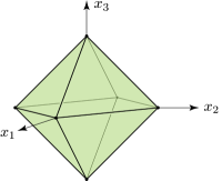
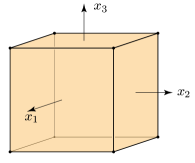
Figure 3: Unit balls ${B}_{\infty,1}^{\top\!\star}$ (left) and ${B}_{1,1}^{\top}$ (right) when $d=3$

  

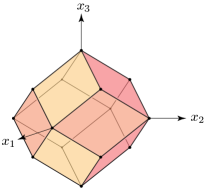
Figure 4: Unit balls ${B}_{\infty,2}^{\top\!\star}$ (left) and ${B}_{1,2}^{\top}$ (right) when $d=3$

When $k$ is equal to $1$, ${B}_{1,k}^{\top}$ coincides with the hypercube $\gamma_{d}$ and ${B}_{\infty,k}^{\top\!\star}$ with the cross-polytope $\beta_{d}$. When $k$ is equal to ${d}$, the opposite holds: ${B}_{1,k}^{\top}$ coincides with the cross-polytope $\beta_{d}$ and ${B}_{\infty,k}^{\top\!\star}$ with the hypercube $\gamma_{d}$. In particular these two families interpolate between the hypercube and the cross-polytope and, as pointed out in [9], ${B}_{1,k}^{\top}$ and ${B}_{\infty,k}^{\top\!\star}$ are related by polarity for all $k$ in $\llbracket 1,{d}\rrbracket$ and not just when $k$ is equal to $1$ or ${d}$. Note that in [9] the parameter $k$ is allowed to take any (possibly non integral) value in the interval $[1,{d}]$. In dimension $3$, these two polytopes are shown on Figure 3 when $k$ is equal to $1$ and in Figure 4 when $k$ is equal to $2$. Theorem 2.1 from [9] can be rephrased as follows.

Theorem 10

The facets of ${B}_{1,k}^{\top}$ are precisely the sets of the form

$$\mathop{\mathrm{co}}\biggl{(}F_{\bot}(\beta_{d},y)\cup{\frac{1}{k}F_{\bot}(\gamma_{d},y)}\biggr{)}$$ (31)

where $y$ is a vector in $\{-1,0,1\}^{d}$ with exactly $k$ nonzero coordinates.

Observe that (31) is precisely $F_{\bot}({B}_{1,k}^{\top},y)$. As noted in [9], for any vector $y$ in $\{-1,0,1\}^{d}$, the affine hulls of $F_{\bot}(\beta_{d},y)$ and $F_{\bot}(\gamma_{d},y)$ are orthogonal subspaces of $\mathbb{R}^{d}$. More precisely, if we denote by $k$ the number of nonzero coordinates of $y$, hence $k=\ell_{0}({y})$, then the two polytopes $F_{\bot}(\beta_{d},y)$ and $F_{\bot}(\gamma_{d},y)/k$ intersect in a single point that belongs to the relative interior of both of these polytopes. We then get, as an immediate consequence, the following description of all the proper faces of ${B}_{1,k}^{\top}$ from Theorem 10.

Corollary 11

The proper faces of ${B}_{1,k}^{\top}$ are precisely the sets of the form

$$\mathop{\mathrm{co}}\biggl{(}F\cup{\frac{1}{k}G}\biggr{)}$$ (32)

where, for some vector $y$ in $\{-1,0,1\}^{d}$ with exactly $k$ nonzero coordinates,

1. $F$ and $G$ are exposed faces of $F_{\bot}(\beta_{d},y)$ and $F_{\bot}(\gamma_{d},y)$, respectively,

2. $F$ and $G$ are not both empty,

3. $F$ is equal to $F_{\bot}(\beta_{d},y)$ if and only if $G$ is equal to $F_{\bot}(\gamma_{d},y)$.

Corollary 11 completely describes the face lattice of ${B}_{1,k}^{\top}$ (which is further enumerated in [9]). Since ${B}_{\infty,k}^{\top\!\star}$ is the polar of ${B}_{1,k}^{\top}$, the normal cones of ${B}_{\infty,k}^{\top\!\star}$ are precisely the cones spanned by the faces of ${B}_{1,k}^{\top}$ and, as a consequence, Corollary 11 also describes the normal fan of ${B}_{\infty,k}^{\top\!\star}$. By the duality between the face lattice of a polytope and its normal fan, one then also recovers the face lattice of ${B}_{\infty,k}^{\top\!\star}$ from that corollary and the normal fan of ${B}_{1,k}^{\top}$.

4.3 The case when $1<p<+\infty$

When the source norm is the $\ell_{p}$-norm where $1<p<+\infty$, the first row of Table 1 tells us that we should study the unit balls of the top-($q$,$k$) norm, with $1/p+1/q=1$, and its dual ($p$,$k$)-support norm. Thus, we will describe the exposed faces and the normal cones of ${B}_{p,k}^{\top\!\star}$. The exposed faces and normal cones of ${B}_{p,k}^{\top}$ can then be recovered by polarity. The balls ${B}_{2,2}^{\top\!\star}$ and ${B}_{2,2}^{\top}$ are shown on Figure 5 when ${d}$ is equal to $3$. One can see that ${B}_{2,2}^{\top}$ is the intersection of three cylinders colored yellow, orange, and red. By duality, ${B}_{2,2}^{\top\!\star}$ has eight triangular faces. While these triangular faces are exposed, their edges, shown as dotted lines, are faces of ${B}_{2,2}^{\top\!\star}$ that are not exposed.

  

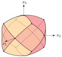
Figure 5: Unit balls ${B}_{2,2}^{\top\!\star}$ (left) and ${B}_{2,2}^{\top}$ (right) when $d=3$

The face of $B_{p}$ exposed by a nonzero vector $y$ from $\mathbb{R}^{d}$ can be recovered from the equality case of Hölder’s inequality. Indeed, by this inequality,

$$\bigl{|}\left\langle z\!\mid\>\!\!y\right\rangle\bigr{|}\leq\|y\|_{q}$$ (33)

for any point $z$ in $B_{p}$ with equality when

$$|z_{i}|^{p}=\lambda|y_{i}|^{q}$$ (34)

for some nonnegative number $\lambda$ and all integers $i$ satisfying $1\leq{i}\leq{d}$, where

$$\frac{1}{p}+\frac{1}{q}=1\;.$$ (35)

Now assume that $z$ belongs to the face of $B_{p}$ exposed by $y$. In that case, $\|z\|_{p}$ is equal to $1$ and (33) must turn into an equality. In particular, there exists a nonnegative number $\lambda$ satisfying (34) for every $i$. The value of $\lambda$ can be recovered by summing (34) over $i$:

$$\lambda=\frac{1}{\|y\|_{q}^{q}}\;.$$ (36)

As a consequence, $z$ must be the point such that, when $y_{i}$ is equal to $0$ then so is $z_{i}$ and when $y_{i}$ is nonzero, then $z_{i}$ is the number with the same sign than $y_{i}$ satisfying

$$|z_{i}|=\biggl{(}\frac{|y_{i}|}{\|y\|_{q}}\biggr{)}^{\!q/p}\;.$$ (37)

Hence, the face of $B_{p}$ exposed by $y$ is made of just the point $z$. From now on, we shall denote $z$ by $v_{p}(y)$. Note that $v_{2}(y)$ and $y$ are collinear, more precisely,

$$v_{2}(y)=\frac{y}{\|y\|_{2}}\;.$$ (38)

We are now able to characterize the exposed faces of ${B}_{p,k}^{\top\!\star}$.

Theorem 12

For any number $p$ satisfying $1<p<+\infty$, the face of ${B}_{p,k}^{\top\!\star}$ exposed by a given nonzero vector $y$ is the convex hull of all the points of the form $v_{p}(\pi_{K^{\sharp}}y)$ where

$$K^{\sharp}\in\mathop{\arg\max}_{{\lvert K\rvert}\leq k}{\|{\pi_{K}y}}\|_{1}\;.$$ (39)

Proof. Using Equation (28) for the orthant-strictly monotonic $\ell_{p}$-norm, one obtains that

$$F_{\bot}\Bigl{(}{B}_{p,k}^{\top\!\star},y\Bigr{)}=\overline{\mathrm{co}}\Big{\{}{F_{\bot}(B_{p},\pi_{K^{\sharp}}y):\,K^{\sharp}\in\mathop{\arg\max}_{{\lvert K\rvert}\leq k}\left\lVert\pi_{K}y\right\rVert_{p}}\Big{\}}\;.$$

Consider any size $k$ subset $K^{\sharp}$ of $\llbracket 1,{d}\rrbracket$ that belongs to ${\mathop{\arg\max}_{{\lvert K\rvert}\leq k}\left\lVert\pi_{K}y\right\rVert_{p}}$. As seen in Equation (37), the face of $B_{p}$ exposed by $\pi_{K^{\sharp}}y$ is the vertex $v_{p}(\pi_{K^{\sharp}}y)$. Hence,

$$F_{\bot}\Bigl{(}{B}_{p,k}^{\top\!\star},y\Bigr{)}=\overline{\mathrm{co}}\Big{\{}{v_{p}(\pi_{K^{\sharp}}y):\,K^{\sharp}\in\mathop{\arg\max}_{{\lvert K\rvert}\leq k}\left\lVert\pi_{K}y\right\rVert_{p}}\Big{\}}\;.$$

Finally, since the $\ell_{p}$-norms are (strictly) monotonic,

$$\mathop{\arg\max}_{{\lvert K\rvert}\leq k}\|\pi_{K}y\|_{p}=\mathop{\arg\max}_{{\lvert K\rvert}\leq k}{\|{\pi_{K}y}}\|_{1}\mbox{,}$$

which completes the proof. $\Box$

Let us first introduce some notation. Consider an integer $k$ in $\llbracket 1,{d}\rrbracket$ and a nonzero vector $y$ from $\mathbb{R}^{d}$. Denote by $m_{k}(y)$ the largest number such that the set

$$\big{\{}{i\in\llbracket 1,{d}\rrbracket:\,|y_{i}|\geq{m_{k}(y)}}\big{\}}$$

contains at least $k$ indices. In other words,

$$m_{k}(y)=\sup\Big{\{}{\lambda\geq 0:\,{\big{\lvert}\{{i\in\llbracket 1,{d}\rrbracket:\,|y_{i}|\geq{\lambda}}\}\big{\rvert}}\geq k}\Big{\}}\;.$$

We will refer by $L_{k}(y)$ to the set of the indices $i$ such that $|y_{i}|$ is greater than $m_{k}(y)$ and by $\overline{L}_{k}(y)$ the set of the indices $i$ such that $|y_{i}|$ is greater than or equal to $m_{k}(y)$:

$$L_{k}(y) =\big{\{}{i\in\llbracket 1,{d}\rrbracket:\,|y_{i}|>m_{k}(y)}\big{\}}\;,$$ (40a)

$$\overline{L}_{k}(y) =\big{\{}{i\in\llbracket 1,{d}\rrbracket:\,|y_{i}|\geq m_{k}(y)}\big{\}}\;.$$ (40b)

The following statement is an immediate consequence of these definitions.

Proposition 13

For any integer $k$ in $\llbracket 1,{d}\rrbracket$ and any nonzero vector $y$ in $\mathbb{R}^{d}$,

$$L_{k}(y)=\bigcap_{K^{\sharp}}K^{\sharp}$$

and

$$\overline{L}_{k}(y)=\bigcup_{K^{\sharp}}K^{\sharp}$$

where the union and the intersection range over the elements $K^{\sharp}$ of $\mathop{\arg\max}_{{\lvert K\rvert}\leq k}\left\lVert\pi_{K}y\right\rVert_{1}$.

Using these notations, Theorem 12 allows to recover the description of the normal cones of ${B}_{p,k}^{\top\!\star}$ given in [19, Proposition 23]. In our setting, the normal cone of ${B}_{p,k}^{\top\!\star}$ at one of its exposed faces $F$ refers to the closure of the set of the vectors $y$ in $\mathbb{R}^{d}$ such that $F$ is the face of ${B}_{p,k}^{\top\!\star}$ exposed by $y$. The normal fans of ${B}_{2,2}^{\top\!\star}$ and ${B}_{2,2}^{\top}$ are illustrated in Fig. 6 when $d$ is equal to $3$. The figure only shows a portion of these fans but both can be reconstructed by symmetry.

  

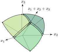
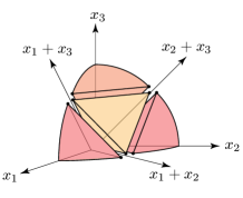
Figure 6: Portions of the normal fan of ${B}_{2,2}^{\top\!\star}$ (left) and of ${B}_{2,2}^{\top}$ (right) when $d=3$

Theorem 14 ([19, Proposition 23])

The normal cones of ${B}_{p,k}^{\top\!\star}$ at its exposed faces are the sets of the form

$$\overline{\mathrm{cone}}{\big{\{}{y\in\mathbb{R}^{d}:\,\pi_{\overline{L}_{k}(z)}y=z,\,\overline{L}_{k}(y)=\overline{L}_{k}(z)}\big{\}}}\;,$$ (41)

where $\overline{\mathrm{cone}}(X)$ denotes the closure of the cone spanned by $X$ and $z$ is a unit vector from $\mathbb{R}^{d}$ such that $z$ coincides with $\pi_{\overline{L}_{k}(z)}z$.

Proof. Consider a nonzero vector $z$ in $\mathbb{R}^{d}$ and denote

$$G=F_{\perp}\Bigl{(}{B}_{p,k}^{\top\!\star},z\Bigr{)}\mbox{.}$$

According to Theorem 12,

$$G=\overline{\mathrm{co}}\Big{\{}{v_{p}(\pi_{K^{\sharp}}z):\,K^{\sharp}\in\mathop{\arg\max}_{{\lvert K\rvert}\leq k}\left\lVert\pi_{K}z\right\rVert_{1}}\Big{\}}\mbox{.}$$ (42)

It suffices to determine all the vectors $y$ such that $G$ is the face of ${B}_{p,k}^{\top\!\star}$ exposed by $y$. First observe that a subset $K^{\sharp}$ of $\llbracket 1,{d}\rrbracket$ belongs to ${\mathop{\arg\max}_{{\lvert K\rvert}\leq k}{\|{\pi_{K}z}}\|_{1}}$ if and only if

$$L_{k}(z)\subset K^{\sharp}\subset\overline{L}_{k}(z)$$ (43)

and either $m_{k}(z)$ is equal to $0$ or $K^{\sharp}$ has exactly $k$ elements. In particular by Theorem 12,

$$G=F_{\perp}\Bigl{(}{B}_{p,k}^{\top\!\star},\pi_{\overline{L}_{k}(z)}z\Bigr{)}\;,$$ (44)

and we can assume, without loss of generality, that $z$ coincides with $\pi_{K^{\sharp}}z$. We will treat two separate cases depending on whether $m_{k}(z)$ is equal to $0$ or not. First, if $m_{k}(z)$ is equal to $0$, then $\overline{L}_{k}(z)$ is equal to $\llbracket 1,{d}\rrbracket$ and (41) just states that the normal cone of ${B}_{p,k}^{\top\!\star}$ at $G$ is the half-line spanned by $z$. However, in that case, Theorem 12 states that $G$ is equal to $\{v_{p}(z)\}$. Hence if $y$ is another nonzero vector such that $G$ is the face of ${B}_{p,k}^{\top\!\star}$ exposed by $y$, the points $v_{p}(z)$ and $v_{p}(y)$ must coincide, which implies that $x$ and $y$ are multiples of one another by a positive factor and that the normal cone of ${B}_{p,k}^{\top\!\star}$ at $G$ is the half-line spanned by $z$, as desired.

Now assume that $m_{k}(z)$ is not equal to $0$ and consider a nonzero vector $y$ such that $G$ is the face of ${B}_{p,k}^{\top\!\star}$ exposed by $y$. It follows from Theorem 12 that

$$G=\overline{\mathrm{co}}\Big{\{}{v_{p}(\pi_{K^{\sharp}}y):\,K^{\sharp}\in\mathop{\arg\max}_{{\lvert K\rvert}\leq k}\left\lVert\pi_{K}y\right\rVert_{1}}\Big{\}}\;.$$ (45)

Consider a subset $K^{\sharp}$ of $\llbracket 1,{d}\rrbracket$ such that

$$K^{\sharp}\in\mathop{\arg\max}_{{\lvert K\rvert}\leq k}\left\lVert\pi_{K}z\right\rVert_{1}\;.$$

Since $m_{k}(z)$ is not equal to $0$, $K^{\sharp}$ contains exactly $k$ elements and $|z_{i}|$ is nonzero when $i$ belongs to $K^{\sharp}$. By construction, a coordinate of $v_{p}(\pi_{K^{\sharp}}z)$ is nonzero if and only if the corresponding coordinate of $\pi_{K^{\sharp}}z$ is nonzero. As a consequence, according to (42), $v_{p}(\pi_{K^{\sharp}}z)$ is the unique vertex of $G$ contained in ${\cal R}_{K^{\sharp}}$. It then follows from (45) that

$$\mathop{\arg\max}_{{\lvert K\rvert}\leq k}\left\lVert\pi_{K}y\right\rVert_{1}=\mathop{\arg\max}_{{\lvert K\rvert}\leq k}\left\lVert\pi_{K}z\right\rVert_{1}\;,$$ (46)

and that, for every set $K^{\sharp}$ contained in $\mathop{\arg\max}_{{\lvert K\rvert}\leq k}\left\lVert\pi_{K}z\right\rVert_{1}$,

$$v_{p}(\pi_{K^{\sharp}}y)=v_{p}(\pi_{K^{\sharp}}z)\;.$$ (47)

According to Proposition 13 and to (46), $\overline{L}_{k}(z)$ and $\overline{L}_{k}(y)$ coincide. Now recall that the normal cones of $B_{p}$ at its proper faces are half lines incident to the origin of $\mathbb{R}^{d}$. Hence, according to (47), there exists a positive number $\alpha_{K^{\sharp}}$ such that

$$\pi_{K^{\sharp}}y=\alpha_{K^{\sharp}}\pi_{K^{\sharp}}z\;.$$

It remains to show that the value of $\alpha_{K^{\sharp}}$ does not depend on $K^{\sharp}$. Indeed, this will imply that up to a positive multiplicative factor, $\pi_{\overline{L}_{k}(z)}y$ coincides with $z$ and results in the desired form (41) for the normal cone of ${B}_{p,k}^{\top\!\star}$ at $G$. If $L_{k}(z)$ is nonempty, this is immediate. Indeed,

$$\alpha_{K^{\sharp}}=\frac{y_{i}}{z_{i}}\;,$$

for any element $i$ of $L_{k}(z)$ and as a consequence, $\alpha_{K^{\sharp}}$ does not depend on $K^{\sharp}$. Therefore, assume that $L_{k}(z)$ is empty. In that case, $z_{i}$ is equal to $m_{k}(z)$ when $i$ belongs to $\overline{L}_{k}(z)$, and equal to $0$ otherwise. Moreover, the sets $K^{\sharp}$ are precisely the size $k$ subsets of $\overline{L}_{k}(z)$. If $k$ is equal to $1$, these sets are all the singletons from $\overline{L}_{k}(z)$ and this implies that $L_{k}(y)$ is also empty. Therefore $y_{i}$ is equal to $m_{k}(y)$ when $i$ belongs to $\overline{L}_{k}(y)$ which implies that $\alpha_{K^{\sharp}}$ does not depend on $K^{\sharp}$.

Finally assume that $k$ is at least $2$ and observe that, for any two nondisjoint size $k$ subsets $K^{\sharp}$ and $\widetilde{K}^{\sharp}$ of $\overline{L}_{k}(z)$, the values of $\alpha_{K^{\sharp}}$ and $\alpha_{\widetilde{K}^{\sharp}}$ necessarily coincide. As $k$ is at least $2$, the graph whose vertices are the size $k$ subsets of $\overline{L}_{k}(z)$ and whose edges connect two of them when they are nondisjoint is connected, it follows that $\alpha_{K^{\sharp}}$ does not depend on $K^{\sharp}$. $\Box$

By analogy with the polytopal case, the normal fan of ${B}_{p,k}^{\top\!\star}$ refers to the set $\mathcal{N}({B}_{p,k}^{\top\!\star})$ of its normal cones. It is a consequence of Theorem 14 that the normal cones, and therefore the normal fan of ${B}_{p,k}^{\top\!\star}$ do not depend on $p$ when $1<p<+\infty$. Interestingly, $B_{p}$ has the same property: its normal cones are $\{0\}$ and the half-lines incident to the origin independently on $p$ when $1<p<+\infty$. We show that $\mathcal{N}({B}_{p,k}^{\top\!\star})$ refines $\mathcal{N}({B}_{\infty,k}^{\top\!\star})$ in the sense of [29, Section 7].

Corollary 15

Every cone from $\mathcal{N}({B}_{p,k}^{\top\!\star})$ is contained in a cone from $\mathcal{N}({B}_{\infty,k}^{\top\!\star})$.

Proof. Since the normal cones of ${B}_{p,k}^{\top\!\star}$ do not depend on $p$, it suffices to prove the statement when $p$ is equal to $2$. Consider a cone $C$ in $\mathcal{N}({B}_{2,k}^{\top\!\star})$. If $C$ is empty or equal to $\{0\}$, then this is immediate. Assume that $C$ is the normal cone of ${B}_{2,k}^{\top\!\star}$ at an exposed face which we will denote by $F$. According to Theorem 14, there exists a nonzero vector $z$ in $\mathbb{R}^{d}$ that coincides with $\pi_{\overline{L}_{k}(z)}z$ such that

$$C=\overline{\mathrm{cone}}{\big{\{}{y\in\mathbb{R}^{d}:\,\pi_{\overline{L}_{k}(z)}y=z,\overline{L}_{k}(y)=\overline{L}_{k}(z)}\big{\}}}\;.$$ (48)

Observe that if $m_{k}(z)$ is equal to $0$, then $\overline{L}_{k}(z)$ is equal to $\llbracket 1,{d}\rrbracket$. In that case, $C$ is the half-line spanned by $z$ and it is contained in a normal cone of ${B}_{\infty,k}^{\top\!\star}$. Therefore, we shall assume from now on that $m_{k}(z)$ is positive. Consider a size $k$ set $K^{\sharp}$ such that $L_{k}(z)\subset{K^{\sharp}}\subset\overline{L}_{k}(z)$. Since $m_{k}(z)$ is positive, $z_{i}$ is nonzero when $i$ belongs to $K^{\sharp}$. Denote by $y$ the vector such that

$$y_{i}=\begin{cases}-1&\mbox{if }z_{i}<0\mbox{ and }i\in{K^{\sharp}}\;,\\ 1&\mbox{if }z_{i}>0\mbox{ and }i\in{K^{\sharp}}\;,\\ 0&\mbox{if }i\not\in{K^{\sharp}}\;.\end{cases}$$ (49)

By construction, $y$ has exactly $k$ nonzero coordinates. Denote

$$F=\mathrm{co}\biggl{(}F_{\bot}(\beta_{d},y)\cup{\frac{1}{k}F_{\bot}(\gamma_{d},y)}\biggr{)}\;.$$ (50)

According to Theorem 10, $F$ is a facet of ${B}_{1,k}^{\top}$. We will show that $C$ is contained in the cone spanned by $F$. By polarity, this cone belongs to $\mathcal{N}({B}_{\infty,k}^{\top\!\star})$ and this will therefore prove the corollary. Consider a vector $x$ such that $\pi_{\overline{L}_{k}(z)}x$ is equal to $z$ and $\overline{L}_{k}(x)$ to $\overline{L}_{k}(z)$. It suffices to show that $x$ belongs to the cone spanned by $F$. Indeed, since that cone is closed, it follows from (48) that $C$ must be contained in it. Observe that $x$ can be decomposed as

$$x=\pi_{K^{\sharp}}x+\pi_{\llbracket 1,{d}\rrbracket\mathord{\setminus}K^{\sharp}}x\;.$$ (51)

By construction, $x_{i}$ is equal to $m_{k}(z)y_{i}$ when $i$ belongs to $K^{\sharp}\mathord{\setminus}L_{k}(z)$. Hence,

$$\pi_{K^{\sharp}}x=\pi_{L_{k}(z)}x-m_{k}(z)\pi_{L_{k}(z)}y+m_{k}(z)y\;.$$ (52)

Since $\pi_{\overline{L}_{k}(z)}x$ is equal to $z$ and $L_{k}(z)$ is a subset of $\overline{L}_{k}(z)$, the first term in the right-hand side is equal to $\pi_{L_{k}(z)}z$. As a consequence $x$ can be rewritten into $x^{\prime}+x^{\prime\prime}$ where

$$\left\{\begin{array}[]{l}x^{\prime}=\pi_{L_{k}(z)}z-m_{k}(z)\pi_{L_{k}(z)}y\;,\\[3.0pt] x^{\prime\prime}=m_{k}(z)y+\pi_{\llbracket 1,{d}\rrbracket\mathord{\setminus}K^{\sharp}}x\;.\end{array}\right.$$ (53)

Observe that $x^{\prime}$ is contained in the cone spanned by $F_{\bot}(\beta_{d},y)$ and $x^{\prime\prime}$ in the cone spanned by $F_{\bot}(\gamma_{d},y)$. Hence, $x^{\prime}+x^{\prime\prime}$ is contained in the cone spanned by $F$, as desired. $\Box$

We recall that the hypersimplex $\delta_{d,k}$ is the convex hull of the vertices of $[0,1]^{d}$ that have exactly $k$ nonzero coordinates. These polytopes appear in algebraic combinatorics [12, 13] and in convex geometry [9, 23, 24]. By extension, we call hypersimplex any polytope that coincides up to a bijective affine transformation, with the convex hull of such a subset of vertices of the hypercube. It is observed in [9] that ${B}_{\infty,k}^{\top\!\star}$ can be decomposed into a union of hypersimplices with pairwise disjoint interiors and that the proper faces of ${B}_{\infty,k}^{\top\!\star}$ are either hypersimplices or isometric copies of ${B}_{\infty,k}^{\top\!\star}$, but for another ambient dimension than ${d}$. The situation for ${B}_{p,k}^{\top\!\star}$ is different as all of its proper faces are hypersimplices.

Corollary 16

If $1<p<+\infty$, then all the proper faces of ${B}_{p,k}^{\top\!\star}$ are hypersimplices.

Proof. Consider a proper face $F$ of ${B}_{p,k}^{\top\!\star}$. Let us first assume that $F$ is exposed by a vector $y$. If $m_{k}(y)$ is equal to $0$, then for every subset $K^{\sharp}$ of $\llbracket 1,{d}\rrbracket$ that belongs to ${\mathop{\arg\max}_{{\lvert K\rvert}\leq k}{\|{\pi_{K}y}}\|_{p}}$,

$$\pi_{K^{\sharp}}y=y$$ (54)

It then follows from Theorem 12 that $F$ is the convex hull of a single point and therefore a $0$-dimensional hypersimplex. Let us now assume that $m_{k}(y)$ is positive.

Denote $|\overline{L}_{k}(y)\mathord{\setminus}L_{k}(y)|$ by $n$ and let us identify $\mathbb{R}^{n}$ with the subspace of $\mathbb{R}^{d}$ made up of the points $x$ such that $x_{i}$ is equal to $0$ when $i$ belongs to either $L_{k}(y)$ or $\llbracket 1,{d}\rrbracket\mathord{\setminus}\overline{L}_{k}(y)$. Denote by $P$ the orthogonal projection of $F$ on $\mathbb{R}^{n}$. It follows from Theorem 12 that $P/m_{k}(y)$ is, up to flipping the signs of the coordinates, the convex hull of the points in $\{0,1\}^{d}$ with exactly $k-|L_{k}(y)|$ nonzero coordinates, as desired.

Now assume that $F$ is not an exposed face of ${B}_{p,k}^{\top\!\star}$. In that case, $F$ is a proper face of an exposed face of ${B}_{p,k}^{\top\!\star}$. Hence by the above, $F$ is proper face of a hypersimplex. As all the proper faces of a hypersimplex are lower-dimensional hypersimplices, this completes the proof. $\Box$

5 Conclusion

Our original motivation was to identify a class of norms which, when added as a penalty term, promote sparsity in an optimization problem, but within a given sparsity budget $k$. For this purpose, we have studied in Sect. 2 the exposed faces of closed convex sets generated by $k$-sparse vectors, hence whose extreme points are $k$-sparse. We also have deduced support identification from dual information. Thus equipped, we have focused in Sect. 3 on the faces of the unit balls of so-called generalized $k$-support norms, constructed from $k$-sparse vectors and from a source norm. In the cases of orthant-monotonic and orthant-strictly monotonic source norms, we have obtained a characterization of the intersection of the $k$-sparse vectors with the faces of the $k$-support norm. Theorem 6 makes the link with our original motivation: we have provided dual conditions under which the primal optimal solution of a minimization problem, penalized by a $k$-support norm, is $k$-sparse. Going back to the original work of Tibshirani [27], the intuition — behind proposing least-square regression with an $\ell_{1}$-norm penalty to achieve sparsity — is that the kinks of the $\ell_{1}$-unit ball are located at sparse points (see Figure 1). In Sect. 4, we have gone on in that direction by providing geometric descriptions of the face and cone lattices of the unit balls of top-($q$,$k$) norm and ($p$,$k$)-support norms. By contrast with the $\ell_{1}$-unit ball, faces intersect in a subtle way, mixing kinks and smoother parts, as illustrated by Figure 5 (left). So, guided by sparsity, we have moved in this paper from optimization to the geometry of unit balls.

Acknowledgements. The third author is partially supported by the Natural Sciences and Engineering Research Council of Canada Discovery Grant program number RGPIN-2020-06846.

References

- [1] A. Argyriou, R. Foygel, and N. Srebro. Sparse prediction with the -support norm. In Proceedings of the 25th International Conference on Neural Information Processing Systems - Volume 1, NIPS’12, pages 1457–1465, USA, 2012. Curran Associates Inc.
- [2] F. Bach, R. Jenatton, J. Mairal, and G. Obozinski. Optimization with sparsity-inducing penalties. Foundations and Trends® in Machine Learning, 4(1):1–106, January 2012.
- [3] H. H. Bauschke and P. L. Combettes. Convex analysis and monotone operator theory in Hilbert spaces. CMS Books in Mathematics/Ouvrages de Mathématiques de la SMC. Springer-Verlag, New York, second edition, 2017.
- [4] C. Boyer, A. Chambolle, Y. De Castro, V. Duval, F. de Gournay, and P. Weiss. On representer theorems and convex regularization. SIAM Journal on Optimization, 29(2):1260–1281, 2019.
- [5] E. J. Candès. The restricted isometry property and its implications for compressed sensing. Comptes Rendus Mathématique, 346(9):589–592, 2008.
- [6] J.-P. Chancelier and M. De Lara. Capra-convexity, convex factorization and variational formulations for the pseudonorm. Set-Valued and Variational Analysis, 30:597–619, 2022.
- [7] J.-P. Chancelier and M. De Lara. Orthant-strictly monotonic norms, generalized top- and -support norms and the pseudonorm. Journal of Convex Analysis, 30(3):743–769, 2023.
- [8] V. Chandrasekaran, B. Recht, P. A. Parrilo, and A. S. Willsky. The convex geometry of linear inverse problems. Foundations of Computational Mathematics, 12(6):805–849, oct 2012.
- [9] A. Deza, J.-B. Hiriart-Urruty, and L. Pournin. Polytopal balls arising in optimization. Contributions to Discrete Mathematics, 16(3):125–138, 2021.
- [10] J. Fadili, J. Malick, and G. Peyré. Sensitivity analysis for mirror-stratifiable convex functions. SIAM Journal on Optimization, 28(4):2975–3000, 2018.
- [11] Z. Fan, H. Jeong, Y. Sun, and M. P. Friedlander. Atomic decomposition via polar alignment. Foundations and Trends® in Optimization, 3(4):280–366, 2020.
- [12] A. M. Gabriélov, I. M. Gel’fand, and M. V. Losik. Combinatorial computation of characteristic classes. Functional Analysis and its Applications, 9:103–115, 1975.
- [13] I. M. Gel’fand, M. Goresky, R. D. MacPherson, and V. Serganova. Combinatorial geometries, convex polyhedra and Schubert cells. Advances in Mathematics, 63:301–316, 1987.
- [14] J.-Y. Gotoh, A. Takeda, and K. Tono. DC formulations and algorithms for sparse optimization problems. Math. Program., 169(1):141–176, may 2018.
- [15] J.-Y. Gotoh and S. Uryasev. Two pairs of families of polyhedral norms versus -norms: proximity and applications in optimization. Math. Program., Ser. A, 156:391–431, 2016.
- [16] D. Gries. Characterization of certain classes of norms. Numerische Mathematik, 10:30–41, 1967.
- [17] D. Gries and J. Stoer. Some results on fields of values of a matrix. SIAM Journal on Numerical Analysis, 4(2):283–300, 1967.
- [18] R. Jenatton, J.-Y. Audibert, and F. Bach. Structured variable selection with sparsity-inducing norms. Journal of Machine Learning Research, 12(84):2777–2824, 2011.
- [19] A. Le Franc, J.-P. Chancelier, and M. De Lara. The capra-subdifferential of the pseudonorm. Optimization, 73(4):1229–1251, 2024.
- [20] A. M. McDonald, M. Pontil, and D. Stamos. New perspectives on -support and cluster norms. Journal of Machine Learning Research, 17(155):1–38, 2016.
- [21] L. Mirsky. Symmetric gauge functions and unitarily invariant norms. The Quarterly Journal of Mathematics, 11(1):50–59, Jan. 1960.
- [22] G. Obozinski and F. Bach. A unified perspective on convex structured sparsity: Hierarchical, symmetric, submodular norms and beyond. Preprint, Dec. 2016.
- [23] L. Pournin. Shallow sections of the hypercube. Israel Journal of Mathematics, 255:685–704, 2023.
- [24] L. Pournin. Local extrema for hypercube sections. Journal d’Analyse Mathématique, 152:557–594, 2024.
- [25] R. T. Rockafellar and R. J.-B. Wets. Variational Analysis. Springer-Verlag, Berlin, 1998.
- [26] R. Schneider. Convex bodies: the Brunn-Minkowski theory. Cambridge University Press, second edition, 2014.
- [27] R. Tibshirani. Regression shrinkage and selection via the lasso. Journal of the Royal Statistical Society. Series B (Methodological), 58(1):267–288, 1996.
- [28] B. Wu, C. Ding, D. Sun, and K.-C. Toh. On the Moreau-Yosida regularization of the vector -norm related functions. SIAM Journal on Optimization, 24(2):766–794, 2014.
- [29] G. M. Ziegler. Lectures on Polytopes, volume 152 of Graduate Texts in Mathematics. Springer, 1995.