Quantum Reservoir Computing and Risk Bounds

Abstract

We propose a way to bound the generalisation errors of several classes of quantum reservoirs using the Rademacher complexity. We give specific, parameter-dependent bounds for two particular quantum reservoir classes. We analyse how the generalisation bounds scale with growing numbers of qubits. Applying our results to classes with polynomial readout functions, we find that the risk bounds converge in the number of training samples. The explicit dependence on the quantum reservoir and readout parameters in our bounds can be used to control the generalisation error to a certain extent. It should be noted that the bounds scale exponentially with the number of qubits $n$. The upper bounds on the Rademacher complexity can be applied to other reservoir classes that fulfill a few hypotheses on the quantum dynamics and the readout function.

Keywords: Quantum Machine Learning, Quantum Reservoir Computing, Rademacher Complexity, Risk Bounds, Generalisation Error

1 Introduction

As an alternative to classical machine learning models, which tend to require a high number of parameters and consequently large data sets, quantum machine learning (QML) models for near-term quantum devices present a promising lead for understanding the potential of quantum technologies. Many current near-term QML methods are based on some form of variational quantum circuits and can be used for different learning tasks, such as classification (Schuld et al. (2020)), autoencoding (Romero et al. (2017)) and generative models (Romero et al. (2019)). Phenomena like barren plateaus (McClean et al. (2018)) and general poor trainability (Anschuetz and Kiani (2022)) of variational quantum methods have motivated the search for circuit designs and quantum machine learning models that circumvent these issues.

Reservoir computing (RC) has recently garnered some attention as an energy and data efficient alternative to more mainstream variants of recurrent neural networks (RNN) for time series forecasting problems (Tanaka et al. (2019); Gilpin (2023)). Instead of a large neural network with trainable weights, RC uses a fixed-weight reservoir described by its input-dependent dynamics and a final readout layer, the latter of which is usually a simple model such as a linear or polynomial regression. The RC models that we are concerned with in this paper possess a memory of past inputs and are able to adapt to the dynamics of the input process. While initially conceived as a type of neural network (Jaeger (2001)), physical implementations of RC such as the use of silicone octopus arms have become a novel way to introduce different reservoir dynamics (Nakajima (2020)).

Two important properties that we typically require of a class of RC models are the so called echo state property (ESP) and the fading memory property (FMP), both of which are characterisations of how the reservoir’s “memory” of past inputs should behave over time. The ESP ensures that the reservoir forgets its initial conditions in the infinite time limit. On the other hand, a reservoir with the FMP will yield similar outputs for two input processes that behaved differently in the distant past but similarly in the recent past.

Recent propositions for quantum reservoir computing (QRC) propose to leverage the complex dynamics of quantum systems to reproduce the behaviour of complex input data dynamics. Since the only trainable part of a quantum reservoir is in the classical linear regression, the trainability issues of other QML models mentioned earlier are no longer of concern. As pointed out by Chen and Nurdin (2019), for the quantum system to have ESP, it must be dissipative (see e.g. Fujii and Nakajima (2016)). As an example, Suzuki et al. (2022) make use of the so called depolarising error.

One of the properties that is often studied in machine learning is a model’s ability to generalise on unseen data. We call the generalisation error or risk of a hypothesis class the expected value of the loss over all possible samples according to some data distribution. Since this distribution is generally unknown, it is bounded through the maximal difference within the class of hypothesis functions between the generalisation error and the empirical error, i.e. the average of the model’s errors evaluated on a finite number of training samples. Essentially, an upper bound on this quantity can give an idea of how different the loss on a random data sample will be, compared to the empirical risk. This upper bound is often called a risk bound. Ideally, the risk bound should decrease as the number of samples in the empirical risk increases. The risk bound can also give some information on how to scale the parameters of the learning model in order to improve its ability to generalise. A common way to bound the risk of a hypothesis class is through the Rademacher complexity, which is essentially a measure of the “richness” of the class by quantifying how well the class can adapt to random noise. The Rademacher complexity is defined on a finite number of samples, and for a hypothesis class to exhibit good generalisation, we expect the Rademacher complexity to go down as the number of samples goes up.

If the hypothesis class is universal, the difference between the in-class minimum and the minimum over all measurable functions can be made arbitrarily small. Formally, a universal class of RC is defined to be a class such that for any process characterised by a dynamical map with fading memory, there exists a member of the reservoir class that can approximate the fading memory map arbitrarily well. Some popular reservoir classes have been proven to be universal by Grigoryeva and Ortega (2018a, b). Universal reservoir classes based on quantum dynamics have been analysed in Chen and Nurdin (2019); Chen et al. (2020); Sannia et al. (2024). Monzania and Pratia (2024) give universality conditions for reservoir classes based on quantum dynamics. For our analysis, we restrict ourselves to quantum reservoir classes with a fixed number of qubits, similarly to Bu et al. (2022), which is a more realistic setting. This is in contrast to the standard procedure when analysing universality properties of quantum reservoir classes where the number of qubits is generally unbounded.

Gonon et al. (2020) propose a certain number of hypotheses which allow them to establish risk bounds for reservoir classes equipped with a general readout class. In this paper, we propose to bound the Rademacher complexity of a general quantum reservoir class with finite parameter space equipped with different readout classes. We show that, under certain constraints, the dynamics of the quantum reservoir, which are governed by completely positive trace preserving (CPTP) maps, verify the aforementioned hypotheses.

We establish risk bounds for different quantum reservoirs and provide an analysis of the scaling of the risk bound in the number of training samples. We show how the choice of the readout class can impact the scaling of the risk bound in the number of qubits. As stated above, the specific classes of quantum reservoirs that we study employ polynomial readouts to prove universality. We show that this choice leads to an unfavourable scaling in the number of qubits. This problem can be somewhat alleviated by choosing either a linear readout function, or a polynomial readout of fixed (small) degree, in a fixed number of variables. Another method to introduce the structure of a polynomial algebra that has been suggested by Sannia et al. (2024) and Monzania and Pratia (2024) is spatial multiplexing. We compare the scaling of a polynomial readout and spatial multiplexing.

The generalisation abilities of certain parameterised quantum circuit configurations have been studied for example by Bu et al. (2022) and Caro et al. (2022), using the Rademacher complexity and covering numbers respectively. The learning problem in these cases is based on independent and identically distributed samples and is thus not immediately applicable to reservoir computing. Gonon and Jacquier (2023) establish approximation error bounds for trainable variational quantum circuits as well as quantum extreme learning machines (a form of reservoir computing that does not take into account past input states) using the Fourier transform. To our knowledge, risk bounds for the specific case of reservoir computing with quantum dynamics for time series forecasting have not yet been studied.

This paper is organised as follows: In Section 2 we introduce the mathematical background and recall some definitions. In Section 3 we establish some general conditions on the quantum reservoir classes as well as the input and target processes. In Section 4 we establish bounds on the Rademacher complexity for any quantum reservoir that verifies the conditions established in Section 3 when equipped with a polynomial readout class, as well as for linear and spatial multiplexing readout classes. In Section 5 we define slightly modified versions of the QRC classes introduced by Chen and Nurdin (2019) and Chen et al. (2020) and show that they verify the hypotheses from Section 3. Finally, in Section 6 we establish risk bounds for the reservoir classes from Section 5 that explicitly depend on the reservoir and readout parameters.

2 Framework

2.1 General definitions

We first define some of the notation that will be used in the remainder of the paper, namely the reservoir system and its filter and functional, the input-output processes, the echo state and fading memory property, which are two important properties of a reservoir system, and some norms that we use in the remainder of the document.

Hilbert Space.

For the Hilbert space $\mathcal{H}=\mathbb{C}^{2^{n}},\,n\in\mathbb{N}$, define the set $\mathcal{B}(\mathcal{H})$ (which we abbreviate as $\mathcal{B}$ in the following) of bounded self-adjoint trace-class linear operators that act on $\mathcal{H}$, as well as the dual space $\mathcal{B}^{*}(\mathcal{H})$ of all possible linear transformations $T(\mathcal{B}):\mathcal{B}\mapsto\mathcal{B}$ which we abbreviate as $\mathcal{B}^{*}$ and which forms a finite Banach space with induced norm $\lVert T\rVert_{1}=\underset{A\in\mathcal{B},A\neq 0}{\text{sup}}\frac{\lVert T(A)\rVert_{1}}{\lVert A\rVert_{1}}$.

Density Matrices.

Define the set of quantum density matrices
$\bar{\mathcal{B}}^{+}(\mathcal{H}):=\{\rho\in\mathcal{B}:\rho\geq 0,\text{tr}[\rho]=1\}$, as well as the hyperplane of traceless operators $\mathcal{B}_{0}(\mathcal{H}):=\left\{A\in\mathcal{B}:\text{tr}\left[A\right]=0\right\}$ which we abbreviate as $\bar{\mathcal{B}}^{+}$ and $\mathcal{B}_{0}$ respectively. In the following we may also call elements in $\bar{\mathcal{B}}^{+}$ quantum states.

Input and Output Sequences.

We now define the classical input and output sequences as well as the quantum reservoir states. Let $\mathbb{Z}_{-}=\{\ldots,-2,-1,0\}$ be the set of all negative integers. We consider the semi-infinite input sequences
$\boldsymbol{v}=(\ldots,v_{-1},v_{0})\in\left(D_{v}\right)^{\mathbb{Z}_{-}}\subset\mathbb{R}^{\mathbb{Z}_{-}}$, where $D_{v}$ is a compact subset of $\mathbb{R}$, and output sequences $\boldsymbol{y}=(\ldots,y_{-1},y_{0})\in\mathbb{R}^{\mathbb{Z}_{-}}$ as well as reservoir states $\boldsymbol{\rho}=(\ldots,\rho_{-1},\rho_{0})\in\left(\bar{\mathcal{B}}^{+}\right)^{\mathbb{Z}_{-}}$.

Input and Output Processes.

To model the stochastic processes of the input and output sequences, we consider random variable inputs $\boldsymbol{V}=(V_{t})_{t\in\mathbb{Z}_{-}}$ and outputs $\boldsymbol{Y}=(Y_{t})_{t\in\mathbb{Z}_{-}}$ with a causal Bernoulli shift structure, i.e. for $q_{v},q_{y}\in\mathbb{N}^{*}$ and measurable functions $G^{v}\colon(\mathbb{R})^{q_{v}}\to D_{v}$ and $G^{y}\colon(\mathbb{R})^{q_{y}}\to\mathbb{R}$ of independent and identically distributed random variables $\xi=\left(\left(\xi_{t}^{v},\xi_{t}^{y}\right)_{t\in\mathbb{Z}_{-}}\right)$ with values in $\mathbb{R}^{q_{v}}\times\mathbb{R}^{q_{y}}$ such that for any $t\in\mathbb{Z}_{-}$ we have

$$\begin{aligned} V_{t}=G^{v}(\ldots,\xi_{t-1}^{v},\xi_{t}^{v})\\ Y_{t}=G^{y}(\ldots,\xi_{t-1}^{y},\xi_{t}^{y})\end{aligned}\;.$$ (1)

See (Dedecker et al., 2007, Section 3.1) for more details on Bernoulli shifts.

Quantum Reservoir System.

The reservoir system is defined by the system of equations

$$\begin{cases}\rho_{t}&=T(v_{t},\rho_{t-1})\\ y_{t}&=h(\rho_{t})\end{cases}$$ (2)

where $h:\mathcal{B}\to\mathbb{R}$ is called the readout function and $T\colon D_{v}\times\mathcal{B}\to\mathcal{B}$ is the completely positive trace preserving (CPTP) map that describes the dynamics of the quantum reservoir. A CPTP map is a completely positive linear mapping that preserves the trace of any operator.

Conceptually, the reservoir at time $t$ is described by its reservoir state $\rho_{t}$ and the subsequent input $v_{t+1}$ is injected into the dynamics of the reservoir, which is left to evolve for some unit of time. At time $t+1$, the new reservoir state $\rho_{t+1}$ encodes all of the previously seen inputs, transformed through the reservoir dynamics (see Fig. 1).

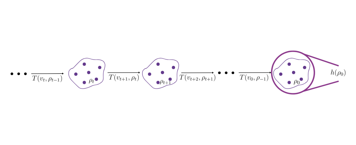
Figure 1: Schematic of the temporal evolution of a quantum reservoir. The purple dots designate qubits, the outline determines the reservoir. At time $t$, the reservoir is in state $\rho_{t}$. A new input $v_{t+1}$ is injected and the full reservoir is made to evolve according to the dynamics induced by the CPTP map $T$. After all the data has been injected in this way, the final reservoir state $\rho_{0}$ is processed in a readout function $h$ which produces the prediction.

Echo State Property.

A reservoir system satisfies the echo state property (ESP) if for any $\boldsymbol{v}\in(D_{v})^{\mathbb{Z}_{-}}$, (2) has a unique solution $\boldsymbol{\rho}\in\left(\bar{\mathcal{B}}^{+}\right)^{\mathbb{Z}_{-}}$ when restricted to the space $\bar{\mathcal{B}}^{+}$ of density matrices. This translates the idea that the reservoir dynamics are independent of its initial conditions.

Reservoir Filter and Functional.

In the case where the system satisfies the ESP, it induces a causal and time invariant reservoir filter $M_{h}^{T}$ as shown by Grigoryeva and Ortega (2018a) which allows us to describe the input transformation of all past inputs, as opposed to the CPTP map which only describes the transformation between time steps $t-1$ and $t$:

$$M_{h}^{T}\colon(D_{v})^{\mathbb{Z}_{-}} \to\mathbb{R}^{\mathbb{Z}_{-}}$$ (3)

$$\boldsymbol{v} \mapsto h\circ M^{T}(\boldsymbol{v})$$ (4)

where $M^{T}(\boldsymbol{v}):=\left(\ldots,T\left(v_{-1},\rho_{-2}\right),T\left(v_{0},\rho_{-1}\right)\right)$, with the corresponding functional

$$H_{h}^{T}\colon(D_{v})^{\mathbb{Z}_{-}} \to\mathbb{R}$$ (5)

$$\boldsymbol{v} \mapsto h\circ H^{T}(\boldsymbol{v})$$ (6)

where we define $H^{T}(\boldsymbol{v}):=M^{T}(\boldsymbol{v})_{0}$, and the subscript $0$ indicates the last element in the semi-infinite sequence, i.e. $M^{T}(\boldsymbol{v})_{0}=T\left(v_{0},\rho_{-1}\right)=\rho_{0}$. The subscript $h$ and superscript $T$ are meant to highlight the dependence of the filter and functional on the CPTP map $T$ and the readout function $h$. In the following we will omit this subscript and superscript of the reservoir functional whenever the dependence on $T$ and $h$ is clear from the definitions.

Fading Memory.

Let $\boldsymbol{w}=\{w_{t}\}_{t\geq 0}$ be a decreasing positive-valued sequence such that $\underset{t\to\infty}{\text{lim}}w_{t}=0$. Then we call the norm $\lVert\cdot\rVert_{1,\boldsymbol{w}}$ defined as $\lVert\boldsymbol{v}\rVert_{1,\boldsymbol{w}}:=\sum_{t\in\mathbb{Z}_{-}}|v_{t}|w_{-t}$ for $\boldsymbol{v}\in(D_{v})^{\mathbb{Z}_{-}}$ the $(1,\boldsymbol{w})$-norm and define the space $\ell_{-}^{1,w}:=\left\{\boldsymbol{v}\in\mathbb{R}^{\mathbb{Z}_{-}}\Big{|}\left\lVert\boldsymbol{v}\right\rVert_{1,\boldsymbol{w}}<\infty\right\}$. We say that a reservoir map has $\boldsymbol{w}$-fading memory if for any $\boldsymbol{v},\boldsymbol{s}\in(D_{v})^{\mathbb{Z}_{-}}$, for all $\varepsilon>0$ there exists $\delta>0$ such that $\left|M_{h}^{T}(\boldsymbol{v})_{0}-M_{h}^{T}(\boldsymbol{s})_{0}\right|<\varepsilon$ whenever $\sup_{t\in\mathbb{Z}_{-}}|v_{t}-s_{t}|w_{-t}<\delta$ (alternatively, we say that a reservoir map has the fading memory property (FMP) if there exists a decreasing positive-valued weighting sequence $\boldsymbol{w}$ such that the reservoir map has $\boldsymbol{w}$-fading memory). This formalises the idea that a reservoir map should focus more on recent inputs and forget the distant past over time.

Norms.

For an operator $\Phi$ we write $\lVert\Phi\rVert_{2}=\sqrt{\text{tr}[\Phi^{{\dagger}}\Phi]}$ for the Schatten-$2$ norm. Note that for a matrix $A$, the Schatten-$2$ norm $\lVert A\rVert_{2}$ is the same as the Frobenius norm $\lVert A\rVert_{F}=\sqrt{\sum_{i,j}A_{ij}^{2}}$ as well as the $L^{2}$-norm of the vectorised matrix $\lVert\text{vec}(A)\rVert_{2}=\sqrt{\sum_{k}(\text{vec}(A))_{k}^{2}}$. For the remainder of the text, we will use the notation $\lVert\cdot\rVert_{2}$ to denote all three of these norms. This is justified by the fact that any CPTP map $T$ is a linear map, meaning that there exists a matrix $\hat{T}$ such that we can write the linear application as a matrix multiplication $T(A)=\hat{T}A$. We also denote by $\vvvert\cdot\vvvert_{2}$ the operator norm induced by the Schatten-$2$ norm, i.e. $\vvvert T\vvvert_{2}:=\mathop{\text{sup}_{\begin{subarray}{c}A\neq 0\end{subarray}}}\frac{\lVert T(A)\rVert_{2}}{\lVert A\rVert_{2}}=\mathop{\text{sup}_{\begin{subarray}{c}\lVert A\rVert_{2}=1\end{subarray}}}\lVert T(A)\rVert_{2}$, and we write $Big\vvvert T\bigr{|}_{\mathcal{B}_{0}}Big\vvvert_{2}:=\mathop{\text{sup}_{\begin{subarray}{c}A\in\mathcal{B}_{0}\\ A\neq 0\end{subarray}}}\frac{\lVert T(A)\rVert_{2}}{\lVert A\rVert_{2}}=\mathop{\text{sup}_{\begin{subarray}{c}A\in\mathcal{B}_{0}\\ \lVert A\rVert_{2}=1\end{subarray}}}\lVert T(A)\rVert_{2}$.

2.2 Empirical Risk and Rademacher Complexity

In this subsection we formally define the generalisation error, which measures the ability of the reservoir to generalise on unseen data, and then introduce the empirical risk. We also define the Rademacher complexity, the measure that we use to bound the generalisation error.

We consider the loss functions $\ell(\hat{y},y)=f(\hat{y}-y)$ where $f:\mathbb{R}\to\mathbb{R}$ is $L_{\ell}$-Lipschitz-continuous and such that $f(0)=0$. Once again, this condition is necessary for the proofs of the theorems in Section 6. For a hypothesis functional $H$, the generalisation error is given by

$$R(H):=\mathop{\mathbb{E}_{\begin{subarray}{c}(\boldsymbol{V},\boldsymbol{Y})\sim P\end{subarray}}}[\ell(H(\boldsymbol{V}),Y_{0})]$$ (7)

where $P$ is the joint distribution of $\boldsymbol{V}$ and $\boldsymbol{Y}$. As this quantity is generally intractable since $P$ is unknown, the standard procedure to bound the generalisation error is to uniformly bound the maximal difference between the true generalisation error and the empirical risk error for some hypothesis class. The empirical risk error $\hat{R}_{m}(H)$ of the hypothesis functional $H$ is typically defined on $m$ independent and identically distributed samples. In the context of time series, we do not usually have such i.i.d. samples; instead, a common way to define the empirical risk is to consider the $m$ subsequences $(V_{-m+1},\ldots,V_{-i-1},V_{-i})$ for $i=0$ to $m-1$ of the input process to construct $m$ samples. Note that the reservoir filter is defined on an infinite sequence, so that we must append the subsequence with zeros. We thus define $\boldsymbol{V}_{-m+1:-i}:=(\ldots,0,0,V_{-m+1},\ldots,V_{-i-1},V_{-i})$ and the empirical risk of hypothesis $H$

$$\hat{R}_{m}(H):=\frac{1}{m}\sum_{i=0}^{m-1}\ell(H(\boldsymbol{V}_{-m+1:-i}),Y_{-i})\ .$$ (8)

The goal of this paper is to bound the quantity

$$\sup_{H\in\mathcal{H}}\left|R(H)-\hat{R}_{m}(H)\right|$$ (9)

for specific classes $\mathcal{H}$ of quantum reservoirs with dependencies in the parameters of the CPTP and readout maps.

One common way to bound (9) is to find a bound that depends on the Rademacher complexity, and to subsequently bound the Rademacher complexity. In the case of time series, the standard definition of the Rademacher complexity needs to be adapted. Usually, the Rademacher complexity is defined on $k$ independent identically distributed samples. In our case, we only have one sample (the time series). We thus make use of the version defined in (Gonon et al., 2020, Section 4.1) which introduces ghost samples, which are “imagined copies” of the input process: For $k\in\mathbb{N}$, denote by $\tilde{\boldsymbol{V}}^{(0)},\ldots,\tilde{\boldsymbol{V}}^{(k-1)}$ independent copies of $\boldsymbol{V}$, then the Rademacher complexity of the hypothesis class $\mathcal{H}$ is defined as

$$\mathcal{R}_{k}(\mathcal{H})=\frac{1}{k}\mathbb{E}\left[\sup_{H\in\mathcal{H}}\left\lVert\sum_{j=0}^{k-1}\varepsilon_{j}H\left(\tilde{\boldsymbol{V}}^{(j)}\right)\right\rVert_{2}\right]$$ (10)

where $\varepsilon_{0},\ldots,\varepsilon_{k-1}$ are independent and identically distributed Rademacher random variables, independent of $\tilde{\boldsymbol{V}}^{(0)},\ldots,\tilde{\boldsymbol{V}}^{(k-1)}$.

3 General Assumptions on the Data Distribution and Quantum Reservoir Classes

In this section, we establish general conditions for the quantum reservoir classes that we wish to analyse. The conditions that we require of the reservoir map are notably contractivity in the space of quantum density matrices and Lipschitz-continuity in the input space, whereas the conditions on the readout map are mostly related to boundedness and Lipschitz-continuity. We also require the parameter space to be finite.

To be able to bound the generalisation error of the reservoir classes that we describe in Section 5, we first recall the assumptions on the data distribution introduced by Gonon et al. (2020):

1. For $I=y,v$ the functional $G^{I}$ as defined in (1) is $L_{I}$-Lipschitz continuous when restricted to $(\ell_{-}^{1,w^{I}}(\mathbb{R}^{q_{I}}),\lVert\cdot\rVert_{1,\boldsymbol{w}^{I}})$ for some strictly decreasing weighting sequence $\boldsymbol{w}^{I}:\mathbb{N}\to(0,1]$ with finite mean, that is, $\sum_{j\in\mathbb{N}}jw_{j}^{I}<\infty$. More specifically, there exists $L_{I}>0$ such that for all $\boldsymbol{u}^{I}=(u_{t}^{I})_{t\in\mathbb{Z}_{-}}\in\ell_{-}^{1,\boldsymbol{w}^{I}}(\mathbb{R}^{q_{I}})$ and $\boldsymbol{s}^{I}=(s_{t}^{I})_{t\in\mathbb{Z}_{-}}\in\ell_{-}^{1,\boldsymbol{w}^{I}}(\mathbb{R}^{q_{I}})$ it holds that

   $$\lVert G^{I}(\boldsymbol{u}^{I})-G^{I}(\boldsymbol{s}^{I})\rVert_{2}\leq L_{I}\lVert\boldsymbol{u}^{I}-\boldsymbol{s}^{I}\rVert_{1,\boldsymbol{w}^{I}}\ .$$ (11)

2. Additionally, let the innovations in (1) satisfy $\mathbb{E}\left[\left\lVert\xi_{0}^{I}\right\rVert_{2}\right]<\infty$ for $I=y,v$.

3. We also assume that $D_{\boldsymbol{w}^{y}}:=\sup_{i\in\mathbb{N}}\frac{w_{i+1}^{y}}{w_{i}^{y}}<1$ and $D_{\boldsymbol{w}^{v}}:=\sup_{i\in\mathbb{N}}\frac{w_{i+1}^{v}}{w_{i}^{v}}<1$ and that there exists $M_{\xi}>0$ such that for all $t\in\mathbb{Z}_{-}$, $\lVert\xi_{t}^{I}\rVert_{2}<M_{\xi}\ ,\$ where $I=v,y$.

We designate the set of conditions on the input-output processes as
$A^{IO}=\left\{(A^{IO}_{1}),(A^{IO}_{2}),(A^{IO}_{3})\right\}$.

3.1 A General Class of Quantum Reservoirs

We begin by defining a general class of quantum reservoirs and readout maps.

First, we suppose that the parameter space $\Theta$ which parameterises the quantum reservoir maps is of finite cardinality:

1. The size of the parameter space $\Theta$ is finite, i.e. $|\Theta|:=\text{Card}(\Theta)<\infty$  .

This condition can always be verified by restricting the parameter space appropriately. We then define, for a fixed number $n$ of qubits, the general class $\mathcal{F}_{n}^{\text{QRC}}(\Theta)$ of parameterised quantum reservoir maps on an $n$-qubit system with parameters in $\Theta$ as the set of CPTP maps $T$ that map a real-valued input $v$ as well as a self-adjoint trace class linear operator $A$ to another self-adjoint trace class linear operator, and that meets the two following conditions:

1. We require all CPTP maps to be $L_{R}$-Lipschitz-continuous on the real-valued closed input interval $D_{v}=\left[a,b\right]\subset\mathbb{R}$, i.e. there exists a constant $0<L_{R}$ such that for all $T^{\theta}\in\mathcal{F}_{n}^{\text{QRC}}(\Theta)$, for any fixed density operator $\rho\in\bar{\mathcal{B}}^{+}$ and any fixed parameter $\theta\in\Theta$, for all inputs $v_{1},v_{2}\in D_{v}$ we have $\left\lVert T^{\theta}(v_{1},\rho)-T^{\theta}(v_{2},\rho)\right\rVert_{2}\leq L_{R}|v_{1}-v_{2}|$.

2. We further require all CPTP maps to be $r$-contractions in the space of density operators, i.e. there exists a constant $0<r<1$ such that for all $T^{\theta}\in\mathcal{F}_{n}^{\text{QRC}}(\Theta)$, for any fixed $v\in D_{v}$ and for any fixed $\theta\in\Theta$, for all $\rho_{1},\rho_{2}\in\bar{\mathcal{B}}^{+}$, we have
   $\left\lVert T^{\theta}(v,\rho_{1})-T^{\theta}(v,\rho_{2})\rVert_{2}\leq r\lVert\rho_{1}-\rho_{2}\right\rVert_{2}$. Note that this condition implies that the reservoir system has ESP and FMP according to (Martinez-Pena and Ortega, 2023, Proposition 1).

We designate the set of conditions on the CPTP maps as $A^{T}=\left\{(A^{T}_{1}),(A^{T}_{2})\right\}$.

Remark 1

In general, we also require the class $\mathcal{F}_{n}^{\text{QRC}}(\Theta)$ to be separable in the space of bounded continuous functions when equipped with the supremum norm so that we can conclude that the supremum over the reservoir class is measurable. In the case of quantum reservoirs, the classes that we consider are always subsets of the set of bounded operators that act on the finite-dimensional Hilbert space $\mathcal{H}$ with fixed number of qubits $n$, which itself is a vector space and becomes a finite-dimensional metric space when equipped with the supremum norm.

We denote by $\mathcal{F}_{n}^{O}$ a general class of readout functions $h:\bar{\mathcal{B}}^{+}\cup 0\to\mathbb{R}$ on an $n$-qubit system (where 0 denotes the $2^{n}\times 2^{n}$ matrix with all zeros) that verifies the following conditions:

1. $\mathcal{F}_{n}^{O}$ contains the zero function.

2. $\mathcal{F}_{n}^{O}$ is separable in the space of bounded continuous functions when equipped with the supremum norm.

3. The maps $h$ in $\mathcal{F}_{n}^{O}$ are $L_{h}$-Lipschitz continuous where there exists $\bar{L}_{h}>0$ such that $L_{h}\leq\bar{L}_{h}$ for all $h\in\mathcal{F}_{n}^{O}$.

4. There exists $L_{h,0}>0$ such that $|h(0)|\leq L_{h,0}$.

We designate the set of conditions on the readout maps as $A^{h}=\left\{(A^{h}_{1}),(A^{h}_{2}),(A^{h}_{3}),(A^{h}_{4})\right\}$

For a CPTP map $T^{\theta}$, we define
$\overrightarrow{\prod}_{i=0}^{\infty}T^{\theta}(v_{-i})\rho_{-\infty}:=\text{lim}_{N\to\infty}T^{\theta}(v_{0},T^{\theta}(v_{-1},\ldots T^{\theta}(v_{-N},\rho_{-N})))$. Then we can write the infinite composition of reservoir maps $T^{\theta}$ as

$$H^{T^{\theta}}(\boldsymbol{v}):=\overrightarrow{\prod}_{i=0}^{\infty}T^{\theta}(v_{-i})\rho_{-\infty}\ .$$ (12)

We then define the general class of reservoir functionals as

$$\mathcal{H}_{n}^{\text{QRC}}:=\left\{H:(D_{v})^{\mathbb{Z}_{-}}\to\mathbb{R}\>|\>H(\boldsymbol{v})=h\left(H^{T^{\theta}}(\boldsymbol{v})\right),h\in\mathcal{F}_{n}^{O},T^{\theta}\in\mathcal{F}_{n}^{\text{QRC}}(\Theta)\right\}\ .$$ (13)

Note that in general these expressions depend on the initial condition $\rho_{-\infty}$. In the following lemma we show that when condition $(A^{T}_{2})$ is met, the expressions are no longer dependent on the initial condition:

Lemma 2

Let $\mathcal{H}_{n}^{\text{QRC}}$ be the general class of reservoir functionals defined in (13). Then, all filters $H\in\mathcal{H}_{n}^{\text{QRC}}$ are independent of the initial state.

Proof  The contractivity condition $(A^{T}_{2})$ necessarily implies the condition on $T$ in (Chen and Nurdin, 2019, Theorem 3), namely that for all inputs $v\in D_{v}$, there exists $\epsilon\in(0,1)$ such that the input-dependent CPTP map $T(v,\cdot)$ restricted to the hyperplane $\mathcal{B}_{0}$ of $2^{n}\times 2^{n}$ traceless Hermitian operators satisfies $Big\vvvert T\bigr{|}_{\mathcal{B}_{0}}Big\vvvert_{2}\leq 1-\varepsilon$. Lemma 2 is a straightforward consequence of (Chen and Nurdin, 2019, Theorem 3) and its following remark, which states that any quantum system that satisfies the aforementioned condition on $T$, applied an infinite number of times, maps any initial state $\rho_{-\infty}$ to the state $\overrightarrow{\prod}_{i=0}^{\infty}T^{\theta}(v_{-i})\left(\frac{I}{2^{n}}\right)$.  

We can thus set the initial reservoir state to be the completely mixed state, i.e. $\rho_{-\infty}=\frac{I}{2^{n}}$, which makes the reservoir maps in (12) independent of the initial condition. This means that our analyses are independent of the initial state, and we can establish general results.

4 Bounds on the Rademacher Complexity for Specific Readout Functions

We now move on to analyse the Rademacher complexity of quantum reservoirs with specific classes of readout functions. We first begin by defining the polynomial readout class since it has been used multiple times to prove universality of quantum reservoirs (see e.g. Chen and Nurdin (2019); Chen et al. (2020)). We find a bound on the Lipschitz constants of the members of the class, which allows us to establish a general bound on the Rademacher complexity of all reservoir classes which employ this readout class, and where the reservoir maps verify the hypotheses highlighted in Section 3. Additionally, we analyse the Rademacher complexity of two alternative readout classes, namely a linear readout and spatial multiplexing and compare them to the Rademacher complexity of the polynomial readout.

4.1 Polynomial Readout Map

The polynomial nature of the readout class used in the reservoir classes by Chen and Nurdin (2019) and Chen et al. (2020) is used to establish universality of the quantum reservoir classes. In fact, a common way to prove universality in the case of reservoirs is to evoke the Stone-Weierstrass theorem, which, amongst other things, requires the class to be an algebra. The polynomial readout class generates a polynomial algebra.

We define a class of multivariate polynomial readout functions with a slight modification to the one mentioned above, specifically with a maximal degree and a bound on the absolute value of the constant bias:

$$\mathcal{F}_{n,R_{\max},C_{\max}}^{\text{poly}}=\Big{\{}h:\bar{\mathcal{B}}^{+}\cup 0\rightarrow\mathbb{R}\>|\>$$ (14)

$$\hskip 14.22636pth(\rho)=C+\sum_{d=1}^{R}\sum_{i_{1}=1}^{n}\sum_{i_{2}=i_{1}+1}^{n}\cdots\sum_{i_{n}=i_{n-1}+1}^{n}\sum_{r_{i_{1}}+\cdots+r_{i_{n}}=d}w_{i_{1},\ldots,i_{n}}^{r_{i_{1}},\ldots,r_{i_{n}}}\text{tr}\left[\sigma_{Z}^{(i_{1})}\rho\right]^{r_{i_{1}}}\cdots\text{tr}\left[\sigma_{Z}^{(i_{n})}\rho\right]^{r_{i_{n}}},$$

$$\hskip 14.22636pt0\leq|C|\leq C_{\max},w_{i_{1},\ldots,i_{n}}^{r_{i_{1}},\ldots,r_{i_{n}}}\in[0,1],1\leq R\leq R_{\max}\Big{\}}$$

where $\text{tr}\left[\sigma_{Z}^{(i)}\rho\right]$ denotes the expectation of the projective measurement along the $Z$-axis on the $i$-th qubit; $C_{\max}$ is a bound on the maximal magnitude of the constant bias $C$; $R$, $R_{\max}$ and the $r_{i}$ are positive valued integers; $R_{\max}$ is a bound on the degree $R$ of the polynomials; and the $w_{i_{1},\ldots,i_{n}}^{r_{i_{1}},\ldots,r_{i_{n}}}$ are real valued weight parameters. The reason for this modification of the readout function is analogous to the reason for the restriction in the number of qubits.

Note that this is a class of polynomials with a constant bound on the maximal degree, meaning that it is a finite dimensional vector space so that it is separable and condition $(A^{h}_{2})$ in Section 3.1 is immediately verified. Additionally, it is clear that this class contains the zero function by setting all parameters to zero, so that condition $(A^{h}_{1})$ is also verified. We also have $\left|h(0)\right|=|C|\leq C_{\max}$ for all $h\in\mathcal{F}_{n,R_{\max},C_{\max}}^{\text{poly}}$ meaning that $(A^{h}_{4})$ is verified. It remains to show condition $(A^{h}_{3})$, and to find an explicit expression for the Lipschitz constant, which we do in the following proposition:

Proposition 3

The polynomial readout class $\mathcal{F}_{n,R_{\max},C_{\max}}^{\text{poly}}$ introduced in (14), with a fixed number $n\in\mathbb{N}$ of qubits, a maximal degree $R_{\max}$ of the polynomial readout, and a bound $C_{\max}$ on the maximal absolute value of the constant term in the readout verifies assumption $(A^{h}_{3})$, i.e. all maps $h\in\mathcal{F}_{n,R_{\max},C_{\max}}^{\text{poly}}$ are Lipschitz-continuous with bounded Lipchitz constants $L_{h}\leq\bar{L}_{h}^{\text{poly}}$, where we write

$$\bar{L}_{h}^{\text{poly}}:=n\sqrt{2^{n}}R_{\max}\cdot\left(\binom{n+R_{\max}}{R_{\max}}-1\right)\ .$$ (15)

The proof is provided in Appendix A. This proposition is used in Section 6 to establish risk bounds for classes of quantum reservoir functionals that employ this readout function. In the following theorem we bound the Rademacher complexity of the general class of reservoir maps that fulfills the general hypotheses laid out in Section 3.1, equipped with the polynomial readout class (14):

Theorem 4

Consider the class of quantum reservoirs
$\mathcal{H}_{n,R_{\max},C_{\max}}^{\text{poly}}:=\left\{H:(D_{v})^{\mathbb{Z}_{-}}\to\mathbb{R}\>|\>H(\boldsymbol{v})=h\left(H^{T^{\theta}}(\boldsymbol{v})\right),h\in\mathcal{F}_{n,R_{\max},C_{\max}}^{\text{poly}},T^{\theta}\in\mathcal{F}_{n}^{\text{QRC}}(\Theta)\right\}$, i.e. the general class of reservoir maps equipped with the polynomial readout class introduced in (14), with a fixed number $n\in\mathbb{N}$ of qubits, a maximal degree $R_{\max}$ of the polynomial readout, and a bound $C_{\max}$ on the maximal absolute value of the constant term in the readout. Then the Rademacher complexity is bounded as

$$\mathcal{R}_{k}\left(\mathcal{H}_{n,R_{\max},C_{\max}}^{\text{poly}}\right)\leq\frac{1}{\sqrt{k}}\left(\left|\Theta\right|\cdot R_{\max}\cdot\left(\binom{n+R_{\max}}{R_{\max}}-1\right)+C_{\max}\right)$$ (16)

for any $k\geq 2$.

The proof is provided in Appendix B.

The size of the parameter space contributes linearly to the Rademacher complexity and can be chosen to fit the desired complexity.

4.2 Alternative Readout Functions

4.2.1 Linear and Fixed-Polynomial Readout

Note that the bound in (16) is unfavourable in both the number of qubits $n$ and the maximal degree of the polynomial $R_{\max}$. One way to alleviate this problem is to restrict the readout class to a low-degree polynomial, or even a linear readout, similar to Yasuda et al. (2023). This would reduce the upper bound on the Rademacher complexity by a factor $\left(\binom{n+R_{\max}}{R_{\max}}-1\right)$:

Corollary 5

Let $\mathcal{F}_{n,C_{\max}}^{\text{lin}}=\left\{h\in\mathcal{F}_{n,R_{\max},C_{\max}}^{\text{poly}}|R=R_{\max}=1\right\}$ be the class of linear readout functions obtained by restricting the maximal polynomial degree in $\mathcal{F}_{n,C_{\max}}^{\text{lin}}$ to one. Consider the class of quantum reservoirs
$\mathcal{H}_{n,C_{\max}}^{\text{lin}}:=\left\{H:(D_{v})^{\mathbb{Z}_{-}}\to\mathbb{R}\>|\>H(\boldsymbol{v})=h\left(H^{T^{\theta}}(\boldsymbol{v})\right),h\in\mathcal{F}_{n,C_{\max}}^{\text{lin}},T^{\theta}\in\mathcal{F}_{n}^{\text{QRC}}(\Theta)\right\}$, i.e. the general class of reservoir maps equipped with the linear readout class. Then the Rademacher complexity is bounded as

$$\mathcal{R}_{k}(\mathcal{H}_{n,C_{\max}}^{\text{lin}})\leq\frac{1}{\sqrt{k}}\left(\left|\Theta\right|\cdot R_{\max}+C_{\max}\right)$$ (17)

for any $k\geq 2$.

Proof  This bound is obtained by simply replacing the number $\left(\binom{n+R}{R}-1\right)$ of sums in the proof of Theorem 4 by one.  

While this significantly reduces the scaling with $n$, this class no longer induces any non-linearity in the measurement outcomes. An intermediary solution between the two previous readout classes that remains non-linear in the measurements but with a more favourable Rademacher complexity than that of (16) can be obtained through spatial multiplexing, which we explore in the next section.

4.2.2 Spatial Multiplexing

Using spatial multiplexing to introduce a polynomial algebra as suggested by Monzania and Pratia (2024) can yield a similar Rademacher upper bound to the bound of the linear readout in (17), under the correct hypotheses: For a total number of qubits $n$, suppose we have a finite number $\ell$ of independent reservoir systems, each with $n/\ell$ qubits (where $\ell$ is such that $n/\ell$ is an integer). After injecting the input into each reservoir system, we consider the resulting reservoir state $\rho$ to be the joint state $\rho=\rho_{1}\otimes\cdots\otimes\rho_{\ell}$ of each individual reservoir state $\rho_{1},\ldots,\rho_{\ell}$. Then the readout function of the complete state is obtained by multiplying linear readouts of the individual states, and adding a constant bias $C$, i.e.

$$h^{\text{SM}}(\rho)=\left(\sum_{i_{1}=1}^{n/\ell}w_{i_{1}}\text{tr}\left[\sigma_{Z}^{(i_{1})}\rho\right]\right)\cdots\left(\sum_{i_{\ell}=\left(\ell-1\right)\frac{n}{\ell}+1}^{n}w_{i_{\ell}}\text{tr}\left[\sigma_{Z}^{(i_{\ell})}\rho\right]\right)+C\ .$$ (18)

This induces the readout class

$$\mathcal{F}_{n,\ell_{\max},C_{\max}}^{\text{SM}}=\Big{\{}h:\bar{\mathcal{B}}^{+}\cup 0\rightarrow\mathbb{R}\>|\>$$ (19)

$$\hskip 14.22636pth^{\text{SM}}(\rho)=C+\sum_{i_{1}=1}^{n/\ell}\sum_{i_{2}=n/\ell+1}^{2n/\ell}\cdots\sum_{i_{\ell}=\left(\ell-1\right)\frac{n}{\ell}+1}^{n}w_{i_{1}}w_{i_{2}}\cdots w_{i_{\ell}}\text{tr}\left[\sigma_{Z}^{(i_{1})}\rho\right]\text{tr}\left[\sigma_{Z}^{(i_{2})}\rho\right]\cdots\text{tr}\left[\sigma_{Z}^{(i_{\ell})}\rho\right],$$

$$\hskip 14.22636pt0\leq|C|\leq C_{\max},w_{i_{j}}\in[0,1],1\leq\ell\leq\ell_{\max},n/\ell\in\mathbb{N}\Big{\}}$$

where $\ell_{\max}$ denotes the maximal number of independent reservoir systems and $C_{\max}$ is an upper bound on the absolute value of the constant bias. Conditions $(A^{h}_{1})$, $(A^{h}_{2})$ and $(A^{h}_{4})$ are verified in the same way as for the readout class $\mathcal{F}_{n,R_{\max},C_{\max}}^{\text{poly}}$ discussed in Section 4.1. Condition $(A^{h}_{3})$ is verified in the following proposition:

Proposition 6

The spatial multiplexing readout class $\mathcal{F}_{n,\ell_{\max},C_{\max}}^{\text{SM}}$ introduced in (19), with a fixed number $n\in\mathbb{N}$ of qubits, a maximal partition $\ell_{\max}$ of the $n$ qubits, and a bound $C_{\max}$ on the maximal absolute value of the constant term in the readout verifies assumption $(A^{h}_{3})$, i.e. all maps $h\in\mathcal{F}_{n,\ell_{\max},C_{\max}}^{\text{SM}}$ are Lipschitz-continuous with bounded Lipchitz constants $L_{h}\leq\bar{L}_{h}^{\text{SM}}$, where we write

$$\bar{L}_{h}^{\text{SM}}:=\ell_{\max}^{5/2}\sqrt{2^{n}}\ .$$ (20)

The proof is provided in Appendix C.

We can bound the Rademacher complexity in a similar way to Theorem 4:

Corollary 7

Consider the class of quantum reservoirs
$\mathcal{H}_{n,\ell_{\max},C_{\max}}^{\text{SM}}:=\left\{H:(D_{v})^{\mathbb{Z}_{-}}\to\mathbb{R}\>|\>H(\boldsymbol{v})=h\left(H^{T^{\theta}}(\boldsymbol{v})\right),h\in\mathcal{F}_{n,\ell_{\max},C_{\max}}^{\text{SM}},T^{\theta}\in\mathcal{F}_{n}^{\text{QRC}}(\Theta)\right\}$, i.e. the general class of reservoir maps equipped with the spatial multiplexing readout class as defined in (19). Then the Rademacher complexity is bounded as

$$\mathcal{R}_{k}(\mathcal{H}_{n,\ell_{\max},C_{\max}}^{\text{SM}})\leq\frac{1}{\sqrt{k}}\left(\left|\Theta\right|\cdot n+C_{\max}\right)$$ (21)

for any $k\geq 2$.

Proof  The proof proceeds analogously to that of Theorem 4, only replacing the sums and indices, which leads to $\ell$ sums of $n/\ell$ indices.  

We can interpret $\ell_{\max}$ to be analogous to $R_{\max}$ in the class $\mathcal{F}_{n,R_{\max},C_{\max}}^{\text{poly}}$, as $\ell_{\max}$ limits the degree of the polynomial in the measurements of the reservoir state. Note that, compared to Theorem 4, there is no dependence in the maximal degree of the polynomial in the bound on the Rademacher complexity.

The scaling of this bound being significantly more favourable than that of the polynomial readout class, it seems that the spatial multiplexing readout is a more interesting readout class in terms of the Rademacher complexity. In general, the reservoir systems of the individual subsystems are governed by different dynamics, so that the remaining results of the paper are not directly applicable to the general spatial multiplexing case. In particular, the tensor product of Lipschitz-continuous maps is not necessarily Lipschitz-continuous, which means that an ensemble of reservoir classes that individually verify the hypotheses $A^{T}$ does not necessarily verify the hypotheses $A^{T}$ when taken as a tensor product. A more thorough analysis is required to establish general risk bounds when using spatial multiplexing. For the remainder of the document we thus consider the polynomial readout class $\mathcal{F}_{n,R_{\max},C_{\max}}^{\text{poly}}$.

Remark 8

In practice, the condition $(A^{\Theta})$ is likely verified for quantum systems, as the accessible parameters are discretised through the limitations on the physical operations that are performed in order to apply the CPTP map. Depending on the chosen quantum system and the achievable precision of the physical operations, the size of the accessible parameter space might be very large, and the upper bound in Theorem 4 may become meaningless. A simple solution consists in restricting the parameter space artificially; the generalisation bounds in Section 6 can be used to choose an appropriately restricted parameter space.

5 Two Specialised Subclasses of Quantum Reservoirs

We now introduce two more specific classes of quantum reservoirs, namely the Partial Trace Reservoir (PTR) and the Random Reinitialisation Reservoir (RRR), which are adaptations of the reservoir classes by Chen and Nurdin (2019) and Chen et al. (2020), respectively. We use the properties of these reservoirs to establish risk bounds in Section 6 that depend on their parameters as well as the parameters of the polynomial readout class $\mathcal{F}_{n,R_{\text{max},C_{\text{max}}}}^{\text{poly}}$ and the number of training samples.

5.1 Partial Trace Reservoir

We now define the PTR subclass of the reservoir map from Chen and Nurdin (2019), which slightly modifies the input injection and readout function from the first proposal of a QRC introduced by Fujii and Nakajima (2016). Modified versions of this class are frequently considered in quantum reservoir computing (see e.g. Yasuda et al. (2023), Sannia et al. (2024)). Conceptually, we inject the input $v$ into the first qubit in the mixed state $\left(v\ket{0}\bra{0}+(1-v)\ket{1}\bra{1}\right)$, then apply a global Hamiltonian on the full system during a time $\tau$, and subsequently reset the first qubit in order to inject the next input; see Fig. 2 for a visual representation.

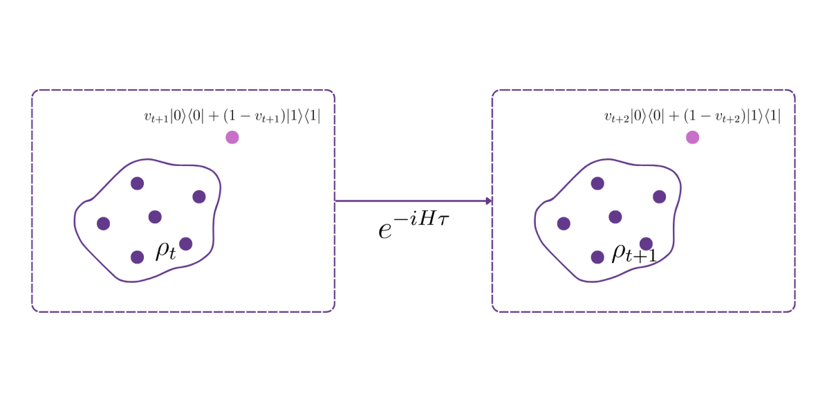
Figure 2: Schematic of the CPTP map of a partial trace reservoir. The purple dots designate the reservoir qubits, the solid outline determines the reservoir. The single pink dot designates the ancillary “input qubit”, and the dashed line designates the system on which we apply the unitary evolution determined by the XY-Hamiltonian. At time $t$, the reservoir is in state $\rho_{t}$. A new input $v_{t+1}$ is injected in the ancillary qubit by setting it to the mixed state $v_{t+1}\ket{0}\bra{0}+(1-v_{t+1})\ket{1}\bra{1}$ and the reservoir qubits along with the ancillary qubit are made to evolve according to the unitary map induced by the Hamiltonian. After time $\tau$, the new reservoir state $\rho_{t+1}$ is obtained by tracing out the ancilla qubit. Finally, the next input is injected into the ancilla qubit.

More concretely, define the input space
$D_{v}^{\text{PTR}}=\left[\frac{1}{2}\left(1-\sqrt{\sqrt{2}-1}\right)+\epsilon_{\text{PTR}},\frac{1}{2}\left(1+\sqrt{\sqrt{2}-1}\right)-\epsilon_{\text{PTR}}\right]$ for some fixed
$0<\epsilon_{\text{PTR}}<\sqrt{\sqrt{2}-1}$. We consider an $n$-qubit system and define the CPTP map

$$T^{J,\gamma,\tau}:D_{v}^{\text{PTR}}\times\mathcal{B} \to\mathcal{B}$$ (22)

$$(v,A) \mapsto\text{tr}_{0}\left[e^{-iH(J,\gamma)\tau}A\otimes\left(v\ket{0}\bra{0}+(1-v)\ket{1}\bra{1}\right)e^{iH(J,\gamma)\tau}\right]$$ (23)

where $\text{tr}_{0}$ denotes the partial trace with respect to the first qubit, $\tau\in\mathbb{R}_{+}$ is a time parameter, and $H(J,\gamma)$ is an $XY$-Hamiltonian of the form

$$H(J,\gamma)=\sum_{i=0}^{n}\sum_{j=i+1}^{n}J^{i,j}\left(\sigma_{X}^{(i)}\sigma_{X}^{(j)}+\sigma_{Y}^{(i)}\sigma_{Y}^{(j)}\right)+\gamma\sum_{i=0}^{n}\sigma_{Z}^{(i)}$$ (24)

where $\sigma_{X}^{(i)},\sigma_{Y}^{(i)}$ and $\sigma_{Z}^{(i)}$ are Pauli-$X$, -$Y$ and -$Z$ matrices applied to the $i$-th qubit (i.e. $\sigma_{X}^{(i)}=I\otimes\cdots\otimes I\otimes\sigma_{X}\otimes I\otimes\cdots\otimes I$ and so on), and the parameters $J=\left\{J^{ij}\right\}$ and $\gamma$ are real-valued constants.

Define $\Theta_{\text{PTR}}$ as the space of such reservoir parameters $J,\gamma$ as well as $\tau\in\mathbb{R}_{+}$. For a fixed number $n$ of qubits, we can then define the class of PTR quantum reservoir maps

$$\mathcal{F}_{n}^{\text{PTR}}:=\left\{T^{J,\gamma,\tau}\>|\>(J,\gamma,\tau)\in\Theta_{\text{PTR}}\right\}\ .$$ (25)

In the following Lemma, we show that the class of reservoir maps $\mathcal{F}_{n}^{\text{PTR}}$ verifies Assumptions $A^{T}$. We use this Lemma in the next section to prove a generalisation bound for the PTR class of quantum reservoirs.

Lemma 9

For any fixed parameters $(J,\gamma,\tau)\in\Theta_{\text{PTR}}$, the CPTP map
$T^{J,\gamma,\tau}:D_{v}^{\text{PTR}}\times\mathcal{B}\to\mathcal{B}\,,\,T^{J,\gamma,\tau}(v,A)\mapsto\text{tr}_{0}\left[e^{-iH(J,\gamma)\tau}A\otimes\left(v\ket{0}\bra{0}+(1-v)\ket{1}\bra{1}\right)e^{iH(J,\gamma)\tau}\right]$ with Hamiltonian $H(J,\gamma)$ is strictly contractive in the space of density operators whenever $0<\epsilon_{\text{PTR}}<\sqrt{\sqrt{2}-1}$, with contractivity constant
$r_{\text{PTR}}(\epsilon_{\text{PTR}})=2\sqrt{2}\left(\epsilon_{\text{PTR}}^{2}-\epsilon_{\text{PTR}}\sqrt{\sqrt{2}-1}\right)+1$. Additionally, the map is Lipschitz-continuous in the space of inputs $D_{v}^{\text{PTR}}$ with Lipschitz-constant $L_{R}^{\text{PTR}}=2$.

The proof is provided in Appendix D. Note that we can somewhat control the strength of the contractivity constant by choosing a convenient value for $\epsilon_{\text{PTR}}$.

In the following, we consider the parameter space $\Theta_{\text{PTR}}$ to be discrete and finite. We then define the class of reservoir functionals associated with the class of PTR reservoir maps as

$$\mathcal{H}_{n,R_{\text{max}},C_{\text{max}}}^{\text{PTR}}\!:=\!\left\{H\!:\!(D_{v})^{\mathbb{Z}_{-}}\!\to\!\mathbb{R}\>|\>H(v)=h\left(H^{T^{J,\gamma,\tau}}(v)\right),h\in\mathcal{F}_{n,R_{\text{max}},C_{\text{max}}}^{\text{poly}},T^{J,\gamma,\tau}\in\mathcal{F}_{n}^{\text{PTR}}\right\}\ .$$ (26)

5.2 Random Reinitialisation Reservoir

We now define the RRR subclass of the reservoir map from Chen et al. (2020), which provides an interesting, more general alternative to the PTR class for quantum platforms on which the Hamiltonian (24) or the input injection in a mixed state are not available. The RRR map can be interpreted as a probabilistic injection of the input $v$, where for some parameter $\alpha\in(0,1)$, with probability $(1-\alpha)v$ we apply the CPTP map $T_{0}$ to the reservoir, and with probability $(1-\alpha)(1-v)$ we apply the CPTP map $T_{1}$ (see Fig. 3 for a visual representation).

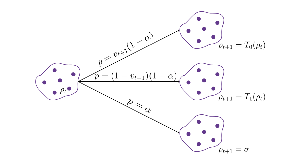
Figure 3: Schematic of the CPTP map of a Random Reintialisation Reservoir. The purple dots designate the reservoir qubits, the solid outline determines the reservoir. At time $t$, the reservoir is in state $\rho_{t}$. With probability $v_{t+1}(1-\alpha)$ we apply the map $T_{0}$ to the reservoir to obtain the new reservoir state $\rho_{t+1}=T_{0}(\rho_{t})$, with probability $(1-v_{t+1})(1-\alpha)$ we apply the map $T_{1}$ to the reservoir to obtain the new reservoir state $\rho_{t+1}=T_{1}(\rho_{t})$, and with probability $\alpha$ we reintialise the reservoir to some fixed quantum state $\sigma$.

Mathematically, define the input space $D_{v}^{\text{RRR}}=\left[\epsilon_{\text{RRR}},\frac{1}{2}-\epsilon_{\text{RRR}}\right]$ for some fixed $0<\epsilon_{\text{RRR}}<\frac{1}{4}$ . We consider an $n$-qubit system and define the CPTP map

$$T^{\alpha,\sigma}:D_{v}^{\text{RRR}}\times\mathcal{B} \to\mathcal{B}$$ (27)

$$(v,A) \mapsto(1-\alpha)\left(vT_{0}+(1-v)T_{1}\right)(A)+\alpha\sigma$$ (28)

where $\sigma$ is a fixed arbitrary quantum state, $\alpha$ is the parameter that determines the probability of reinitialising the reservoir state to $\sigma$ and $T_{0}\neq T_{1}$ are fixed CPTP maps, contractive in the space of density matrices, with contraction constants $r_{0}$ and $r_{1}$ such that $r_{0}+r_{1}<1$. If $r_{0}=r_{1}$, we write $r_{0}=r_{1}=r_{0,1}$. If $r_{0}\neq r_{1}$, we impose $r_{0}>r_{1}$.

For a fixed number $n$ of qubits, we can then define the class of RRR quantum reservoir maps

$$\mathcal{F}_{n}^{\text{RRR}}:=\{T^{\alpha,\sigma}\>|\>(\alpha,\sigma)\in\Theta_{\text{RRR}}\}$$ (29)

where $\Theta_{\text{RRR}}:=[\alpha_{\min},\alpha_{\max}]\times\Sigma$ is some compact subset of $(0,1)\times\bar{\mathcal{B}}^{+}$.

In the following Lemma we show that the class of reservoir maps $\mathcal{F}_{n}^{\text{RRR}}$ verifies Assumptions $A^{T}$. We use this Lemma in the next section to prove a generalisation bound for the RRR class of quantum reservoirs.

Lemma 10

The class of RRR quantum reservoir maps $\mathcal{F}_{n}^{\text{RRR}}$ defined in (29) verifies assumptions $A^{T}$. More specifically, any CPTP map $T^{\alpha,\sigma}\in\mathcal{F}_{n}^{\text{RRR}}$ with arbitrary $n$ is strictly contractive in the space of density operators. If $r_{0}=r_{1}=r_{0,1}$, the contractivity constant is given by $r_{\text{RRR}}=(1-\alpha_{\min})r_{0,1}$. If $r_{0}>r_{1}$, the contractivity constant is given by $r_{\text{RRR}}=1-\epsilon_{\text{RRR}}$. Furthermore, any CPTP map $T^{\alpha,\sigma}\in\mathcal{F}_{n}^{\text{RRR}}$ with arbitrary $n$ is Lipschitz-continuous in the space of inputs $D_{v}^{\text{RRR}}$ with Lipschitz-constant $L_{R}^{\text{RRR}}=2(1-\alpha_{\min})$.

The proof is provided in Appendix E.

In the following, we consider the parameter space $\Theta_{\text{RRR}}$ to be discrete and finite. Finally, we define the class of reservoir functionals associated with the class of RRR reservoir maps as

$$\mathcal{H}_{n,R_{\max},C_{\max}}^{\text{RRR}}\!:=\!\left\{H\!:\!\left(D_{v}^{\text{RRR}}\right)^{\mathbb{Z}_{-}}\!\to\!\mathbb{R}\>\Big{|}\>H(\boldsymbol{v})=h\left(H^{T^{\alpha,\sigma}}(\boldsymbol{v})\right),h\in\mathcal{F}_{n,R_{\max},C_{\max}}^{\text{poly}},T^{\alpha,\sigma}\in\mathcal{F}_{n}^{\text{RRR}}\right\}\ .$$ (30)

Using the results of this section as well as the previous sections, we can derive an upper bound on the generalisation error of the RRR and PTR quantum reservoir classes.

6 Generalisation Bounds of the Quantum Reservoir Classes

We are now ready to present the main results. We can apply (Gonon et al., 2020, Theorem 14) to the RRR and PTR reservoirs, with the appropriate constants. To highlight the dependence in the reservoir parameters, and to simplify notation, we omit the dependencies on parameters that are not determined by the reservoir map or the readout map. The explicit expressions can be found in Appendix H.

Theorem 11

Let $n\in\mathbb{N}$ be a fixed number of qubits. Consider the PTR class of reservoir functionals $\mathcal{H}_{n,R_{\text{max}},C_{\text{max}}}^{\text{PTR}}$ defined in (26) as well as the input and target processes defined in Section 2, fulfilling the hypotheses $A^{IO}$. Assume that Assumption $(A^{\Theta})$ is verified, with $|\Theta_{\text{PTR}}|$ the size of the parameter space. Define $\zeta_{\text{max}}:=\text{max}(r_{\text{PTR}}(\epsilon_{\text{PTR}}),D_{w^{y}},D_{w^{v}})$. Then for all $m\in\mathbb{N}$ such that $\log(m)<m\log(\zeta_{\text{max}}^{-1})$ and for all $\delta\in(0,1)$, with probability at least $1-\delta$ we have

$$\ \sup_{H\in\mathcal{H}_{n,R_{\max},C_{\max}}^{\text{PTR}}}\left|R(H)-\hat{R}_{m}(H)\right|$$ (31)

$$\leq\mathcal{O}\left(\bar{L}_{h}^{\text{poly}}\text{max}\left\{\frac{P_{1}^{p}}{m}\ ,\ P_{2}^{p}\frac{\log{m}}{m}\ ,\ P_{3}^{p}\sqrt{\frac{\log{m}}{m}}\ ,\ P_{4}^{p}\sqrt{\frac{\log{4/\delta}}{2m}}\right\}\right)$$ (32)

where the reservoir parameter dependent expressions are given by

$$P_{1}^{p}=\text{max}\left\{\frac{r_{\text{PTR}}(\epsilon_{\text{PTR}})}{1-r_{\text{PTR}}(\epsilon_{\text{PTR}})}\,,\,2L_{\ell}\zeta_{\text{max}}^{-1}\,,\,L_{\ell}C_{y}\zeta_{\text{max}}^{-1}\right\}$$ (33)

$$P_{2}^{p}=\text{max}\left\{1\,,\,C_{\text{max}}\,,\,2\zeta_{\text{max}}^{-1}C_{v}\right\}$$ (34)

$$P_{3}^{p}=\frac{1}{\bar{L}_{h}^{\text{poly}}\sqrt{\log{\zeta_{\text{max}}^{-1}}}}\max\left\{\left|\Theta_{\text{PTR}}\right|\cdot R_{\max}\cdot\left(\binom{n+R_{\max}}{R_{\max}}-1\right),C_{\max}\right\}$$ (35)

$$P_{4}^{p}=\frac{1}{1-r_{\text{PTR}}(\epsilon_{\text{PTR}})}\text{max}\left\{r_{\text{PTR}}(\epsilon_{\text{PTR}})\,,\,2M_{\xi}L_{v}\left\lVert w^{v}\right\rVert_{1}\right\}$$ (36)

and $\bar{L}_{h}^{\text{poly}}$ is as in (15), i.e. $\bar{L}_{h}^{\text{poly}}=R_{\text{max}}\cdot n\sqrt{2^{n}}\left(\binom{n+R_{\text{max}}}{R_{\text{max}}}-1\right)$.

The proof can be found in Appendix F.

We can proceed analogously for the RRR reservoir class, distinguishing the case where $r_{0}=r_{1}$ from the case where $r_{0}>r_{1}$ to obtain the following result:

Theorem 12

Let $n\in\mathbb{N}$ be a fixed number of qubits. Consider the RRR class of reservoir functionals $\mathcal{H}_{n,R_{\max},C_{\max}}^{\text{RRR}}$ defined in (30) as well as the input and target processes defined in Section 2, fulfilling the hypotheses $A^{IO}$. Assume that Assumption $(A^{\Theta})$ is verified, with $|\Theta_{\text{RRR}}|$ the size of the parameter space. Define $\zeta_{\max}:=\max(r_{\text{RRR}},D_{w^{y}},D_{w^{v}})$. Then for all $m\in\mathbb{N}$ such that $\log(m)<m\log(\zeta_{\max}^{-1})$ and for all $\delta\in(0,1)$, with probability at least $1-\delta$ we have

$$\sup_{H\in\mathcal{H}_{n,R_{\max},C_{\max}}^{\text{RRR}}}\left|R(H)-\hat{R}_{m}(H)\right|$$ (37)

$$\leq\mathcal{O}\left(\bar{L}_{h}^{\text{poly}}\max\left\{\frac{P_{1}^{r}}{m},\ P_{2}^{r}\frac{\log{m}}{m}\ ,\ P_{3}^{r}\sqrt{\frac{\log{m}}{m}}\ ,\ P_{4}^{r}\sqrt{\frac{\log{4/\delta}}{2m}}\right\}\right)$$ (38)

where the reservoir parameter dependent expressions are given by

$$P_{1}^{r}=\begin{cases}\max\left\{\frac{(1-\alpha_{\min})r_{0,1}}{1-(1-\alpha_{\min})r_{0,1}}\ ,\ 1\right\}&\text{ if }r_{0}=r_{1}=r_{0,1}\\ \max\left\{\frac{1-\epsilon_{\text{RRR}}}{\epsilon_{\text{RRR}}}\ ,\ 1\right\}&\text{ if }r_{0}>r_{1}\\ \end{cases}$$ (39)

$$P_{2}^{r}=\max\left\{1\ ,\ 2(1-\alpha_{\min})\zeta_{\max}^{-1}L_{\ell}C_{v}\ ,\ C_{\max}L_{\ell}\right\}$$ (40)

$$P_{3}^{r}=\frac{1}{\bar{L}_{h}^{\text{poly}}\sqrt{\log{\zeta_{\text{max}}^{-1}}}}\max\left\{\left|\Theta_{\text{RRR}}\right|\cdot R_{\max}\cdot\left(\binom{n+R_{\max}}{R_{\max}}-1\right),C_{\max}\right\}$$ (41)

$$P_{4}^{r}=\begin{cases}\frac{\left(1-\alpha_{\min}\right)}{1-\left(\alpha_{\min}\right)r_{0,1}}\max\left\{r_{0,1}\ ,\ 2M_{\xi}L_{v}\left\lVert w^{v}\right\rVert_{1}\right\}&\text{ if }r_{0}=r_{1}=r_{0,1}\\ \frac{1}{\epsilon_{\text{RRR}}}\max\left\{1-\epsilon_{\text{RRR}}\ ,\ 2\left(1-\alpha_{\min}\right)M_{\xi}L_{v}\left\lVert w^{v}\right\rVert_{1}\right\}&\text{ if }r_{0}>r_{1}\\ \end{cases}$$ (42)

and $\bar{L}_{h}^{\text{poly}}$ is as in (15), i.e. $\bar{L}_{h}^{\text{poly}}=R_{\max}\cdot n\sqrt{2^{n}}\left(\binom{n+R_{\max}}{R_{\max}}-1\right)$.

The proof can be found in Appendix G.

From the above theorems we see that the main scaling issues of the generalisation error with respect to the number of qubits comes from the Lipschitz constant of the polynomial readout.

Remark 13

Note that we have analysed the generalisation error in an idealised setting, without taking into account the estimation of the observables. In reality, multiple shots are necessary to average over the measurement results. The risk bound presented in this paper can help prevent overfitting in the idealised setting of stationary time series without noise.

7 Discussion

In this paper, we have established bounds on the Rademacher complexity of a general class of quantum reservoir maps with different readout classes, as well as risk bounds for the more specific quantum reservoir classes which we have introduced in Section 5, based on the classes introduced by Chen and Nurdin (2019) and Chen et al. (2020).

If one wants to use the aforementioned classes for a forecasting task, our risk bounds can give an idea on how to choose a convenient set of parameters that are more likely to generalise well.

On the one hand, we find risk bounds that scale as $\mathcal{O}(\sqrt{\log{m}/m})$ in the number of training samples $m$, which suggests a convergence rate for the generalisation error. On the other hand, our analysis shows that the choice of the class of readout maps can significantly influence the way that the risk bound scales with the number of qubits. As shown in Section 6, the choice of a polynomial readout class leads to the risk bounds scaling as $\mathcal{O}(n\sqrt{2^{n}}\binom{n+R_{\max}}{R_{\max}})$ for a fixed number of qubits $n$, where $R_{\max}$ is an upper bound on the degree of the polynomial. As discussed in Section 4.2, this problem can be somewhat alleviated by choosing either a linear readout function, or a polynomial readout of fixed (small) degree, in a fixed number of variables.

The risk bounds we provide are not directly comparable to the risk bounds established for universal classical reservoir classes, since the modified quantum reservoir classes studied here are a priori no longer universal.

The bad scaling of the risk bound in the number of qubits motivates the search for universal reservoir classes that do not require a polynomial readout class. Grigoryeva and Ortega (2018a) have shown that the reservoir class called State Affine System (SAS) is universal even with a linear readout. Martinez-Pena and Ortega (2023) showed that all input-dependent quantum reservoir maps can be written in a similar form, and thus universality results from Grigoryeva and Ortega (2018a) can be applied to reservoir systems with linear readouts when the necessary conditions are verified. However, verifying these conditions is not trivial; apart from the difficulty of finding explicit matrix representations of the CPTP maps, which is necessary to apply the results from Martinez-Pena and Ortega (2023), establishing risk bounds on those representations is not an easy undertaking, as these matrices necessarily depend on the input variables, making it difficult to separate inputs and reservoir states in the decomposition of the reservoir functional.

Another potential avenue is to utilise the rather general results in Sannia et al. (2024) which establishes conditions on the Lindbladian for the reservoir class to be universal when using spatial multiplexing. In forthcoming work, we develop device-specific classes that can harness the natural dynamics of specific quantum systems, including experimental verification of the theoretical results.

Acknowledgments and Disclosure of Funding

This work was supported by the European Union’s Horizon 2020 research and innovation programs under grant agreement No. 817482 (PASQuanS) and No. 101079862 (PASQuanS2) as well as the ANR projects Q-COAST (ANR-19-CE48-0003) and IGNITION (ANR-21-CE47-0015). Part of this research was conducted during a visit to the Institute for Mathematical and Statistical Innovation (IMSI), which is supported by the National Science Foundation (Grant No. DMS-1929348). The authors would like to thank Paulin Jacquot for useful discussions and technical advice.

Appendix A Proof of Proposition 3

In the following we show that all readout functions in the class $\mathcal{F}_{n,R_{\max},C_{\max}}^{\text{poly}}$ are Lipschitz-continuous in the space of square $2^{n}\times 2^{n}$ matrices $\rho$ with $\text{tr}\left[\sigma_{Z}^{(i)}\rho\right]\in[-1,1]$ for all $i$, with Lipschitz-constants bounded by $\bar{L}_{h}^{\text{poly}}$ as defined in (15).

Let $\rho_{1},\rho_{2}\in\bar{\mathcal{B}}^{+}\cup 0$ be two density matrices or the square $2^{n}\times 2^{n}$ matrix with only zero entries. Denote by $g_{i}(\rho):=\text{tr}\left[\sigma_{Z}^{(i)}\rho\right]\in[-1,1]$ the expectation of operator $\sigma_{Z}^{(i)}$ (i.e. of the measurement operator of the $i$-th qubit on the $Z$-axis). The function $g_{i}$ is a Lipschitz-continuous function with Lipschitz-constant $\sqrt{2^{n}}$ for all $i$, since

$$\left|\text{tr}(\sigma_{Z}^{(i)}\rho_{1})-\text{tr}(\sigma_{Z}^{(i)}\rho_{2})\right| =\left|\text{tr}(\sigma_{Z}^{(i)}(\rho_{1}-\rho_{2}))\right|$$ (43)

$$\leq\sqrt{\text{tr}(\sigma_{Z}^{(i)^{{\dagger}}}\sigma_{Z}^{(i)})}\sqrt{\text{ tr }((\rho_{1}-\rho_{2})^{{\dagger}}(\rho_{1}-\rho_{2}))}$$ (44)

$$=\sqrt{2^{n}}\lVert\rho_{1}-\rho_{2}\rVert_{2}$$ (45)

where we have used linearity of the trace operator and matrix multiplication in the first step, the Cauchy-Schwarz inequality in the second step, and the fact that $\sigma_{Z}^{(i)}$ is hermitian and unitary in the last step.

Next, define

$$f(x_{i_{1}},\ldots x_{i_{n}})=w_{i_{1},\ldots,i_{n}}^{r_{i_{1}},\ldots,r_{i_{n}}}(x_{i_{1}})^{r_{i_{1}}}\cdots(x_{i_{n}})^{r_{i_{n}}}$$ (46)

where $x_{i_{k}}\in[-1,1]$ for all $i_{k}$. Then for each $x_{i_{k}}$, the partial derivative of $f(x_{i_{1}},\ldots x_{i_{n}})$ with respect to $x_{i_{k}}$ is

$$D_{x_{i_{k}}}f(x_{i_{1}},\ldots x_{i_{n}})=w_{i_{1},\ldots,i_{n}}^{r_{i_{1}},\ldots,r_{i_{n}}}r_{i_{k}}(x_{i_{1}})^{r_{i_{1}}}\cdots(x_{i_{k}})^{r_{i_{k}-1}}\cdots(x_{i_{n}})^{r_{i_{n}}}\ .$$ (47)

It follows that for each $x_{i_{k}}$, $\rVert D_{x_{i_{k}}}f(x_{i_{1}},\ldots x_{i_{n}})\lVert_{2}\leq\mathop{\max_{\begin{subarray}{c}i_{1},\ldots,i_{n}\\ r_{i_{1}},\ldots,r_{i_{n}}\end{subarray}}}|w_{i_{1},\ldots,i_{n}}^{r_{i_{1}},\ldots,r_{i_{n}}}|\cdot R\leq R$. Recall that an everywhere differentiable multivariate function is Lipschitz continuous if it has bounded partial derivatives, in which case the Lipschitz constant is given by the square root of the sum of the square of the upper bounds of the partial derivatives. That means that the Lipschitz constant $L_{f}$ of $f$ is given by

$$L_{f}=\sqrt{S_{i_{1}}^{2}+\ldots+S_{i_{n}}^{2}}$$ (48)

where $S_{i_{k}}$ is the upper bound of the $i$th partial derivative, i.e. $R$ in our case. This can be shown by applying the mean-valued theorem in multiple variables as well as the Cauchy-Schwarz inequality, see for example (Eriksson et al., 2003, Theorem 54.2 and following discussion). Thus, the function $f$ is Lipschitz-continuous with Lipschitz constant $L_{f}=\sqrt{n}\cdot R$. Then we can write

$$\lVert f(g_{1}(\rho_{1}),\ldots,g_{n}(\rho_{1}))-f(g_{1}(\rho_{2}),\ldots,g_{n}(\rho_{2}))\rVert_{2}$$ (49)

$$\leq L_{f}\left\lVert(g_{1}(\rho_{1})-g_{1}(\rho_{2}),\ldots,g_{n}(\rho_{1})-g_{n}(\rho_{2}))\right\rVert_{2}$$ (50)

$$=L_{f}\sqrt{(g_{1}(\rho_{1})-g_{1}(\rho_{2}))^{2}+\dots+(g_{n}(\rho_{1})-g_{n}(\rho_{2}))^{2}}$$ (51)

$$\leq L_{f}\sqrt{n\cdot 2^{n}\lVert\rho_{1}-\rho_{2}\rVert_{2}^{2}}=n\cdot R\cdot\sqrt{2^{n}}\lVert\rho_{1}-\rho_{2}\rVert_{2}\ .$$ (52)

Note that the sum of Lipschitz-continuous functions is Lipschitz-continuous, where the Lipschitz constant is the sum of the Lipschitz constants of the individual summands. In our case, all summands have the same Lipschitz-constant $L_{f,g}=R\cdot n\sqrt{2^{n}}$ so that the Lipschitz-constant $L_{h}$ of $h$ is simply $L_{f,g}$ multiplied by the number of summands. To find this number, note that the way the $r_{i_{1}},\ldots,r_{i_{n}}$ are partitioned is in fact a known combinatorics problem, called stars and bars or multichoose. The problem is formulated as follows: For a fixed number $d$ of stars, and a fixed number $n$ of bins (delimited by $n-1$ bars), how many ways are there to distribute the $d$ stars into the $n$ bins (allowing empty bins). Then the number of ways to partition the integer $d$ into an $n$-tuple is given by $\binom{n+d-1}{d}$, see for example (Feller, 1968, Chapter II.5). Summing over $d=1,\cdots,R$, we can then bound the complete Lipschitz-constant of $h$ by

$$L_{h}\leq R\cdot n\sqrt{2^{n}}\left(\binom{n+R}{R}-1\right)\ .$$ (53)

In particular, this is bounded by

$$\bar{L}_{h}^{\text{poly}}=R_{\max}\cdot n\sqrt{2^{n}}\left(\binom{n+R_{\max}}{R_{\max}}-1\right)\ .$$ (54)

Appendix B Proof of Theorem 4

For the class $\mathcal{H}_{n,R_{\max},C_{\max}}^{\text{poly}}$ of quantum reservoir functionals, begin by writing

$$\mathbb{E}\left[\sup_{H\in\mathcal{H}_{n,R_{\max},C_{\max}}^{\text{poly}}}\left|\sum_{j=0}^{k-1}\varepsilon_{j}H\left(\tilde{\boldsymbol{V}}^{(j)}\right)\right|\right]$$ (55)

$$=\mathbb{E}\left[\sup_{h\in\mathcal{F}_{n,R_{\max},C_{\max}}^{\text{poly}}\atop T^{\theta}\in\mathcal{F}_{n}^{\text{QRC}}(\Theta)}\left|\sum_{j=0}^{k-1}\varepsilon_{j}h\left(\overrightarrow{\prod}_{i=0}^{\infty}T^{\theta}\left(\tilde{V}^{(j)}_{-i}\right)\rho_{-\infty}\right)\right|\right]$$ (56)

$$=\mathbb{E}\Bigg{[}\sup_{\begin{subarray}{c}w_{i_{1},\ldots,i_{n}}^{r_{i_{1}},\ldots,r_{i_{n}}}\in[0,1]\\ 1\leq R\leq R_{\max}\ ,\ 0\leq|C|\leq C_{\max}\end{subarray}}\sup_{\theta\in\Theta}\Bigg{|}\sum_{j=0}^{k-1}\varepsilon_{j}\Bigg{(}C$$ (57)

$$\hskip 28.45274pt+\sum_{d=1}^{R}\sum_{i_{1}=1}^{n}\sum_{i_{2}=i_{1}+1}^{n}\!\cdots\!\sum_{i_{n}=i_{n-1}+1}^{n}\sum_{r_{i_{1}}+\cdots+r_{i_{n}}=d}w_{i_{1},\ldots,i_{n}}^{r_{i_{1}},\ldots,r_{i_{n}}}\text{tr}\left[\sigma_{Z}^{(i_{1})}\rho_{0}^{\theta,j}\right]^{r_{i_{1}}}\cdots\text{tr}\left[\sigma_{Z}^{(i_{n})}\rho_{0}^{\theta,j}\right]^{r_{i_{n}}}\Bigg{)}\Bigg{|}\Bigg{]}$$ (58)

where we have written $\rho_{0}^{\theta,j}:=\overrightarrow{\prod}_{i=0}^{\infty}T^{\theta}\left(\tilde{V}^{(j)}_{-i}\right)\rho_{-\infty}$. Using the triangle inequality as well as the subadditivity of the supremum, we can bound the last term as follows:

$$\mathbb{E}\Bigg{[}\sup_{\begin{subarray}{c}w_{i_{1},\ldots,i_{n}}^{r_{i_{1}},\ldots,r_{i_{n}}}\in[0,1]\\ 1\leq R\leq R_{\max}\ ,\ 0\leq|C|\leq C_{\max}\end{subarray}}\sup_{\theta\in\Theta}\Bigg{|}\sum_{j=0}^{k-1}\varepsilon_{j}\Bigg{(}C+$$ (59)

$$\hskip 28.45274pt\sum_{d=1}^{R}\sum_{i_{1}=1}^{n}\sum_{i_{2}=i_{1}+1}^{n}\cdots\sum_{i_{n}=i_{n-1}+1}^{n}\sum_{r_{i_{1}}+\cdots+r_{i_{n}}=d}w_{i_{1},\ldots,i_{n}}^{r_{i_{1}},\ldots,r_{i_{n}}}\text{tr}\left[\sigma_{Z}^{(i_{1})}\rho_{0}^{\theta,j}\right]^{r_{i_{1}}}\cdots\text{tr}\left[\sigma_{Z}^{(i_{n})}\rho_{0}^{\theta,j}\right]^{r_{i_{n}}}\Bigg{)}\Bigg{|}\Bigg{]}$$ (60)

$$\leq\mathbb{E}\left[\sup_{\begin{subarray}{c}0\leq|C|\leq C_{\max}\end{subarray}}\left|\sum_{j=0}^{k-1}\varepsilon_{j}C\right|\right]$$ (61)

$$+\mathbb{E}\Bigg{[}\sup_{1\leq R\leq R_{\max}}\sum_{d=1}^{R}\sum_{i_{1}=1}^{n}$$ (62)

$$\hskip 28.45274pt\!\cdots\!\sum_{i_{n}=i_{n-1}+1}^{n}\sum_{r_{i_{1}}+\cdots+r_{i_{n}}=d}\sup_{w_{i_{1},\ldots,i_{n}}^{r_{i_{1}},\ldots,r_{i_{n}}}\in[0,1]\atop\theta\in\Theta}\left|\sum_{j=0}^{k-1}\varepsilon_{j}w_{i_{1},\ldots,i_{n}}^{r_{i_{1}},\ldots,r_{i_{n}}}\text{tr}\left[\sigma_{Z}^{(i_{1})}\rho_{0}^{\theta,j}\right]^{r_{i_{1}}}\!\cdots\!\text{tr}\left[\sigma_{Z}^{(i_{n})}\rho_{0}^{\theta,j}\right]^{r_{i_{n}}}\right|\Bigg{]}\ .$$ (63)

For the first term, we can write

$$\left(\mathbb{E}\left[\sup_{\begin{subarray}{c}0\leq|C|\leq C_{\max}\end{subarray}}\left|\sum_{j=0}^{k-1}\varepsilon_{j}C\right|\right]\right)^{2}\leq\mathbb{E}\left[\sup_{0\leq|C|\leq C_{\max}}\left|C\right|^{2}\left|\sum_{j=0}^{k-1}\varepsilon_{j}\right|^{2}\right]=\sum_{j=0}^{k-1}\mathbb{E}\left[\varepsilon_{j}^{2}\right]C_{\max}^{2}=kC_{\max}^{2}$$ (64)

where we used Jensen’s inequality twice in the first inequality, as well as the fact that $C$ is independent of $j$ and the submultiplicativity of the norm; and the fact that $\mathbb{E}[\varepsilon_{j}\varepsilon_{m}]=0$ if $m\neq j$ in the first equality.

For the second term (63), we write

$$\mathbb{E}\Bigg{[}\sup_{1\leq R\leq R_{\max}}\sum_{d=1}^{R}\sum_{i_{1}=1}^{n}$$ (65)

$$\hskip 28.45274pt\cdots\sum_{i_{n}=i_{n-1}+1}^{n}\sum_{r_{i_{1}}+\cdots+r_{i_{n}}=d}\sup_{w_{i_{1},\ldots,i_{n}}^{r_{i_{1}},\ldots,r_{i_{n}}}\in[0,1]\atop\theta\in\Theta}\left|\sum_{j=0}^{k-1}\varepsilon_{j}w_{i_{1},\ldots,i_{n}}^{r_{i_{1}},\ldots,r_{i_{n}}}\text{tr}\left[\sigma_{Z}^{(i_{1})}\rho_{0}^{\theta,j}\right]^{r_{i_{1}}}\cdots\text{tr}\left[\sigma_{Z}^{(i_{n})}\rho_{0}^{\theta,j}\right]^{r_{i_{n}}}\right|\Bigg{]}$$ (66)

$$\leq\sum_{d=1}^{R_{\max}}\sum_{i_{1}=1}^{n}\cdots\sum_{i_{n}=i_{n-1}+1}^{n}\!\sum_{r_{i_{1}}+\cdots+r_{i_{n}}=d}\mathbb{E}\left[\sup_{w_{i_{1},\ldots,i_{n}}^{r_{i_{1}},\ldots,r_{i_{n}}}\in[0,1]\atop\theta\in\Theta}\left|\sum_{j=0}^{k-1}\varepsilon_{j}w_{i_{1},\ldots,i_{n}}^{r_{i_{1}},\ldots,r_{i_{n}}}\text{tr}\left[\sigma_{Z}^{(i_{1})}\rho_{0}^{\theta,j}\right]^{r_{i_{1}}}\cdots\text{tr}\left[\sigma_{Z}^{(i_{n})}\rho_{0}^{\theta,j}\right]^{r_{i_{n}}}\right|\right]\ .$$ (67)

We can once again take arguments that are independent of $j$ out of the sum and use the submultiplicativity of the norm to bound the term behind the sums:

$$\mathbb{E}\left[\sup_{w_{i_{1},\ldots,i_{n}}^{r_{i_{1}},\ldots,r_{i_{n}}}\in[0,1]\atop\theta\in\Theta}\left|\sum_{j=0}^{k-1}\varepsilon_{j}w_{i_{1},\ldots,i_{n}}^{r_{i_{1}},\ldots,r_{i_{n}}}\text{tr}\left[\sigma_{Z}^{(i_{1})}\rho_{0}^{\theta,j}\right]^{r_{i_{1}}}\cdots\text{tr}\left[\sigma_{Z}^{(i_{n})}\rho_{0}^{\theta,j}\right]^{r_{i_{n}}}\right|\right]$$ (68)

$$=\mathbb{E}\left[\sup_{w_{i_{1},\ldots,i_{n}}^{r_{i_{1}},\ldots,r_{i_{n}}}\in[0,1]\atop\theta\in\Theta}\left|w_{i_{1},\ldots,i_{n}}^{r_{i_{1}},\ldots,r_{i_{n}}}\sum_{j=0}^{k-1}\varepsilon_{j}\text{tr}\left[\sigma_{Z}^{(i_{1})}\rho_{0}^{\theta,j}\right]^{r_{i_{1}}}\cdots\text{tr}\left[\sigma_{Z}^{(i_{n})}\rho_{0}^{\theta,j}\right]^{r_{i_{n}}}\right|\right]$$ (69)

$$\leq\mathbb{E}\left[\sup_{w_{i_{1},\ldots,i_{n}}^{r_{i_{1}},\ldots,r_{i_{n}}}\in[0,1]\atop\theta\in\Theta}\left|w_{i_{1},\ldots,i_{n}}^{r_{i_{1}},\ldots,r_{i_{n}}}\right|\left|\sum_{j=0}^{k-1}\varepsilon_{j}\text{tr}\left[\sigma_{Z}^{(i_{1})}\rho_{0}^{\theta,j}\right]^{r_{i_{1}}}\cdots\text{tr}\left[\sigma_{Z}^{(i_{n})}\rho_{0}^{\theta,j}\right]^{r_{i_{n}}}\right|\right]$$ (70)

$$\leq\mathbb{E}\left[\sup_{\theta\in\Theta}\left|\sum_{j=0}^{k-1}\varepsilon_{j}\text{tr}\left[\sigma_{Z}^{(i_{1})}\rho_{0}^{\theta,j}\right]^{r_{i_{1}}}\cdots\text{tr}\left[\sigma_{Z}^{(i_{n})}\rho_{0}^{\theta,j}\right]^{r_{i_{n}}}\right|\right]\ .$$ (71)

Using the fact that the parameter space is finite, we write

$$\mathbb{E}\left[\sup_{\theta\in\Theta}\left|\sum_{j=0}^{k-1}\varepsilon_{j}\text{tr}\left[\sigma_{Z}^{(i_{1})}\rho_{0}^{\theta,j}\right]^{r_{i_{1}}}\cdots\text{tr}\left[\sigma_{Z}^{(i_{n})}\rho_{0}^{\theta,j}\right]^{r_{i_{n}}}\right|\right]$$ (72)

$$\leq\sum_{\theta\in\Theta}\mathbb{E}\left[\left|\sum_{j=0}^{k-1}\varepsilon_{j}\text{tr}\left[\sigma_{Z}^{(i_{1})}\rho_{0}^{\theta,j}\right]^{r_{i_{1}}}\cdots\text{tr}\left[\sigma_{Z}^{(i_{n})}\rho_{0}^{\theta,j}\right]^{r_{i_{n}}}\right|\right]\ .$$ (73)

We can bound the term behind the sum over the parameter space as follows:

$$\left(\mathbb{E}\left[\left|\sum_{j=0}^{k-1}\varepsilon_{j}\text{tr}\left[\sigma_{Z}^{(i_{1})}\rho_{0}^{\theta,j}\right]^{r_{i_{1}}}\cdots\text{tr}\left[\sigma_{Z}^{(i_{n})}\rho_{0}^{\theta,j}\right]^{r_{i_{n}}}\right|\right]\right)^{2}$$ (74)

$$\leq\mathbb{E}\left[\left|\sum_{j=0}^{k-1}\varepsilon_{j}\text{tr}\left[\sigma_{Z}^{(i_{1})}\rho_{0}^{\theta,j}\right]^{r_{i_{1}}}\cdots\text{tr}\left[\sigma_{Z}^{(i_{n})}\rho_{0}^{\theta,j}\right]^{r_{i_{n}}}\right|^{2}\right]$$ (75)

$$=\sum_{j=0}^{k-1}\mathbb{E}\left[\varepsilon_{j}^{2}\right]\mathbb{E}\left[\left|\text{tr}\left[\sigma_{Z}^{(i_{1})}\rho_{0}^{\theta,j}\right]^{r_{i_{1}}}\cdots\text{tr}\left[\sigma_{Z}^{(i_{n})}\rho_{0}^{\theta,j}\right]^{r_{i_{n}}}\right|^{2}\right]$$ (76)

$$\leq k$$ (77)

where we used Jensen’s inequality in the first inequality, independence between the Rademacher variables and the input variables and the fact that $\mathbb{E}[\varepsilon_{j}\varepsilon_{m}]=0$ if $m\neq j$ in the first equality, as well as the fact that $\text{tr}\left[\sigma_{Z}^{(i)}\rho_{0}^{\theta,j}\right]^{r_{i}}\in[-1,1]$ .

Finally, combining (72) and (74), and using the same combinatorial argument as in Appendix A to bound the number of terms of sums in (67), we have

$$\sum_{d=1}^{R_{\max}}\sum_{i_{1}=1}^{n}\!\cdots\!\sum_{i_{n}=i_{n-1}+1}^{n}\sum_{r_{i_{1}}+\cdots+r_{i_{n}}=d}\mathbb{E}\left[\sup_{w_{i_{1},\ldots,i_{n}}^{r_{i_{1}},\ldots,r_{i_{n}}}\in[0,1]\atop\theta\in\Theta}\left|\sum_{j=0}^{k-1}\varepsilon_{j}w_{i_{1},\ldots,i_{n}}^{r_{i_{1}},\ldots,r_{i_{n}}}\text{tr}\left[\sigma_{Z}^{(i_{1})}\rho_{0}^{\theta,j}\right]^{r_{i_{1}}}\!\cdots\!\text{tr}\left[\sigma_{Z}^{(i_{n})}\rho_{0}^{\theta,j}\right]^{r_{i_{n}}}\right|\right]$$ (78)

$$\leq R_{\max}\left(\binom{n+R_{\max}}{R_{\max}}-1\right)|\Theta|\sqrt{k}\ .$$ (79)

Combining this with (64), we get the final result.

Appendix C Proof of Proposition 6

The proof of Proposition 6 proceeds similarly to the proof of Proposition 3, with a few modifications in the constants.

First, define the multivariate function

$$f(x_{i_{1}},\ldots,x_{i_{\ell}})=w_{i_{1}}\cdots w_{i_{\ell}}x_{i_{1}}\cdots x_{i_{\ell}}\ .$$ (80)

Then, the partial derivatives of $f$ with respect to each variable $x_{i_{k}}$ is given by

$$D_{x_{i_{k}}}f(x_{i_{1}},\ldots,x_{i_{\ell}})=w_{i_{1}}\cdots w_{i_{\ell}}x_{i_{1}}\cdots x_{i_{k-1}}x_{i_{k+1}}\cdots x_{i_{\ell}}$$ (81)

and for each variable $x_{i_{k}}$ the partial derivative is bounded by

$$\left|D_{x_{i_{k}}}f(x_{i_{1}},\ldots,x_{i_{\ell}})\right|\leq\left|w_{i_{1}}\right|\cdots\left|w_{i_{\ell}}\right|\leq 1$$ (82)

where the last inequality follows from the fact that $\left|w_{i_{j}}\right|\leq 1$ by design. Using the same argument as in Appendix A, we conclude that the function $f$ is Lipschitz-continuous with Lipschitz constant $L_{f}=\ell$.

Then, with the functions $g_{i}(\rho)$ as defined in Appendix A and following a similar argument as in (49), we can write

$$\lVert f(g_{1}(\rho_{1}),\ldots,g_{\ell}(\rho_{1}))-f(g_{1}(\rho_{2}),\ldots,g_{\ell}(\rho_{2}))\rVert_{2}$$ (83)

$$\leq L_{f}\left\lVert(g_{1}(\rho_{1})-g_{1}(\rho_{2}),\ldots,g_{\ell}(\rho_{1})-g_{\ell}(\rho_{2}))\right\rVert_{2}$$ (84)

$$=L_{f}\sqrt{(g_{1}(\rho_{1})-g_{1}(\rho_{2}))^{2}+\dots+(g_{\ell}(\rho_{1})-g_{\ell}\rho_{2}))^{2}}$$ (85)

$$\leq L_{f}\sqrt{{\ell}\cdot 2^{n}\lVert\rho_{1}-\rho_{2}\rVert_{2}^{2}}=\ell\cdot\sqrt{{\ell}\cdot 2^{n}}\lVert\rho_{1}-\rho_{2}\rVert_{2}\ .$$ (86)

Finally, by noting that there are $\ell$ sums in the readout function $h^{\text{SM}}$, we conclude that $h^{\text{SM}}$ is Lipschitz-continuous w.r.t. $\rho$, with Lipschitz constant $L_{h}^{\text{SM}}=\ell^{5/2}\sqrt{2^{n}}$, and an upper bound on the Lischitz constants of the class $\mathcal{F}_{n,R_{\max},C_{\max}}^{\text{SM}}$ is given by

$$\bar{L}_{h}^{\text{SM}}=\ell_{\max}^{5/2}\sqrt{2^{n}}\ .$$ (87)

Appendix D Proof of Lemma 9

We begin by proving contractivity in the space of density operators. The proof makes use of (Rastegin, 2012, Proposition 1), which states that for an operator $\tilde{Q}$ defined on a composite system $\mathcal{H}_{A}\otimes\mathcal{H}_{B}$ with $\text{dim}(\mathcal{H}_{A})=m$ and $\text{dim}(\mathcal{H}_{B})=n$ we have

$$\left\lVert\text{tr}_{B}\left[\tilde{Q}\right]\right\rVert_{2}\leq\sqrt{n}\left\lVert\tilde{Q}\right\rVert_{2}\ .$$ (88)

To show that there exists an $r_{\text{PTR}}\in(0,1)$ such that for fixed parameters $(J,\alpha,\gamma)$, for any two quantum states $\rho_{1},\rho_{2}$ and for all $v\in D_{v}$

$$\left\lVert T^{J,\gamma,\tau}(v,\rho_{1})-T^{J,\gamma,\tau}(v,\rho_{2})\right\rVert_{2}\leq r_{\text{PTR}}\left\lVert\rho_{1}-\rho_{2}\right\rVert_{2}\ ,$$ (89)

note that $T^{J,\gamma,\tau}$ is a linear map, and $\rho_{1},\rho_{2}$ being quantum states, we have $\text{tr}[\rho_{1}-\rho_{2}]=0$ so that we can restrict $T^{J,\gamma,\tau}$ to the hyperplane $\mathcal{B}_{0}$ of $2^{n}\times 2^{n}$ traceless Hermitian operators. In the remainder of this proof we write $T=T^{J,\gamma,\tau}$ and $H=H(J,\gamma)\tau$ for ease of notation, as the parameters do not intervene in the calculations. Define $\mathcal{V}=\begin{pmatrix}v&0\\ 0&1-v\end{pmatrix}$. Using (88) we have for all $A\in\mathcal{B}_{0}$,

$$\left\lVert T(v,A)\right\rVert_{2}=\left\lVert\text{tr}_{0}[e^{-iH}A\otimes\mathcal{V}e^{iH}]\right\rVert_{2}\leq\sqrt{2}\left\lVert e^{-iH}A\otimes\mathcal{V}e^{iH}\right\rVert_{2}\ .$$ (90)

Notice also that

$$\left\lVert e^{-iH}A\otimes\mathcal{V}e^{iH}\right\rVert_{2} =\left\lVert A\otimes\mathcal{V}\right\rVert_{2}=\sqrt{\text{tr}\left[\left[A\otimes\mathcal{V}\right]^{*}\left[A\otimes\mathcal{V}\right]\right]}$$ (91)

$$=\sqrt{\text{tr}\left[A^{*}A\otimes\mathcal{V}^{*}\mathcal{V}\right]}=\sqrt{\text{tr}\left[A^{*}A\right]\text{tr}\left[\mathcal{V}^{*}\mathcal{V}\right]}=\left\lVert A\right\rVert_{2}\left(v^{2}+(1-v)^{2}\right)\ .$$ (92)

We thus have, for $v\in\left[\frac{1}{2}(1-\sqrt{\sqrt{2}-1})+\epsilon_{\text{PTR}},\frac{1}{2}(1+\sqrt{\sqrt{2}-1})-\epsilon_{\text{PTR}}\right]$,

$$\sup_{A\in\mathcal{B}_{0}\atop\left\lVert A\right\rVert_{2}=1}\left\lVert T(v,A)\right\rVert_{2}\leq r_{\text{PTR}}(\epsilon_{\text{PTR}})$$ (93)

with

$$r_{\text{PTR}}(\epsilon_{\text{PTR}}) =\sqrt{2}\left(\left(\frac{1}{2}(1+\sqrt{\sqrt{2}-1})-\epsilon_{\text{PTR}}\right)^{2}+\left(1-\frac{1}{2}(1+\sqrt{\sqrt{2}-1})+\epsilon_{\text{PTR}}\right)^{2}\right)$$ (94)

$$=2\sqrt{2}\left(\epsilon_{\text{PTR}}^{2}-\epsilon_{\text{PTR}}\sqrt{\sqrt{2}-1}\right)+1$$ (95)

where we indicate the dependence of the contractivity constant on the choice of $\epsilon_{\text{PTR}}$ We proceed similarly to prove Lipschitz-continuity: For any inputs $v_{1},v_{2}\in D_{v}$ and any density matrix $\rho\in\bar{\mathcal{B}}^{+}$ we have

$$\left\lVert T(v_{1},\rho)-T(v_{2},\rho)\right\rVert_{2}$$ (96)

$$=\left\lVert\text{tr}_{0}\left[e^{-iH}\rho\otimes\begin{pmatrix}v_{1}&0\\ 0&1-v_{1}\end{pmatrix}e^{iH}\right]-\text{tr}_{0}\left[e^{-iH}\rho\otimes\begin{pmatrix}v_{2}&0\\ 0&1-v_{2}\end{pmatrix}e^{iH}\right]\right\rVert_{2}$$ (97)

$$=\left\lVert\text{tr}_{0}\left[e^{-iH}\rho\otimes\begin{pmatrix}v_{1}&0\\ 0&1-v_{1}\end{pmatrix}e^{iH}-e^{-iH}\rho\otimes\begin{pmatrix}v_{2}&0\\ 0&1-v_{2}\end{pmatrix}e^{iH}\right]\right\rVert_{2}$$ (98)

$$=\left\lVert\text{tr}_{0}\left[e^{-iH}\left(\rho\otimes\begin{pmatrix}v_{1}&0\\ 0&1-v_{1}\end{pmatrix}-\rho\otimes\begin{pmatrix}v_{2}&0\\ 0&1-v_{2}\end{pmatrix}\right)e^{iH}\right]\right\rVert_{2}$$ (99)

$$=\left\lVert\text{tr}_{0}\left[e^{-iH}\rho\otimes\begin{pmatrix}v_{1}-v_{2}&0\\ 0&v_{2}-v_{1}\end{pmatrix}e^{iH}\right]\right\rVert_{2}$$ (100)

$$\leq\sqrt{2}\left\lVert\rho\otimes\begin{pmatrix}v_{1}-v_{2}&0\\ 0&v_{2}-v_{1}\end{pmatrix}\right\rVert_{2}$$ (101)

$$=\sqrt{2\text{tr}\left[\left(\rho^{{\dagger}}\otimes\begin{pmatrix}v_{1}-v_{2}&0\\ 0&v_{2}-v_{1}\end{pmatrix}\right)\left(\rho\otimes\begin{pmatrix}v_{1}-v_{2}&0\\ 0&v_{2}-v_{1}\end{pmatrix}\right)\right]}$$ (102)

$$=\sqrt{2\text{tr}\left(\rho^{{\dagger}}\rho\right)\text{tr}\left(\begin{pmatrix}v_{1}-v_{2}&0\\ 0&v_{2}-v_{1}\end{pmatrix}^{2}\right)}$$ (103)

$$\leq\sqrt{2\cdot 2(v_{1}-v_{2})^{2}}=2\lVert v_{1}-v_{2}\rVert_{2}$$ (104)

where the second equality follows from the linearity of the partial trace operator, the first inequality follows from (88), and the second inequality follows from the fact that the purity of any quantum state is bounded by one.

Appendix E Proof of Lemma 10

We begin by proving contractivity in the space of density operators: For any $\rho_{1},\rho_{2}\in\bar{\mathcal{B}}^{+}$ and for any fixed $v\in D_{v}^{\text{RRR}}$ we have

$$\left\lVert T^{\alpha,\sigma}(v,\rho_{1})-T^{\alpha,\sigma}(v,\rho_{2})\right\rVert_{2}$$ (105)

$$=(1-\alpha)\left\lVert(vT_{0}+(1-v)T_{1})\rho_{1}-(vT_{0}+(1-v)T_{1})\rho_{2}\right\rVert_{2}$$ (106)

$$\leq(1-\alpha)(v\left\lVert T_{0}(\rho_{1})-T_{0}(\rho_{2})\right\rVert_{2}+(1-v)\left\lVert T_{1}(\rho_{1})-T_{1}(\rho_{2})\right\rVert_{2})$$ (107)

$$\leq(1-\alpha)(vr_{0}+(1-v)r_{1})\left\lVert\rho_{1}-\rho_{2}\right\rVert_{2}$$ (108)

$$=(1-\alpha)(v(r_{0}-r_{1})+r_{1})\left\lVert\rho_{1}-\rho_{2}\right\rVert_{2}$$ (109)

where we used the fact that $T_{0}$ and $T_{1}$ are $r_{0}$- and $r_{1}$-contractions, respectively. If $r_{0}=r_{1}=r_{0,1}$, the result is immediate noting that $\alpha\in[\alpha_{\min},\alpha_{\max}]\subset(0,1)$. If $r_{0}>r_{1}$, we have $1>r_{0}+r_{1}$ which implies $0<r_{0}-r_{1}<1-2r_{1}$, thus

$$v(r_{0}-r_{1})+r_{1}<v(1-2r_{1})+r_{1}=r_{1}(1-2v)+v<1-v<1-\epsilon_{\text{RRR}}$$ (110)

where the second to last inequality follows from the fact that $r_{1}<1$ and $v<1/2$.

The proof of the Lipschitz-continuity is a straightforward application of the triangle inequality. For any $v_{1},v_{2}\in D_{v}^{\text{RRR}}$ and for any fixed $\rho\in\bar{\mathcal{B}}^{+}$ we have

$$\left\lVert T^{\alpha,\sigma}(v_{1},\rho)-T^{\alpha,\sigma}(v_{2},\rho)\right\rVert_{2}$$ (111)

$$=\left\lVert(1-\alpha)\left(v_{1}T_{0}+(1-v_{1})T_{1}\right)\rho+\alpha\sigma-(1-\alpha)\left(v_{2}T_{0}+(1-v_{2})T_{1}\right)\rho-\alpha\sigma\right\rVert_{2}$$ (112)

$$\leq(1-\alpha)\left\lVert(v_{1}-v_{2})T_{0}(\rho)+(v_{2}-v_{1})T_{1}(\rho)\right\rVert_{2}$$ (113)

$$\leq(1-\alpha)\left|v_{1}-v_{2}\right|\left\lVert T_{0}(\rho)+T_{1}(\rho)\right\rVert_{2}$$ (114)

$$\leq(1-\alpha)\left|v_{1}-v_{2}\right|\left(\left\lVert T_{0}(\rho)\right\rVert_{2}+\left\lVert T_{1}(\rho_{1})\right\rVert_{2}\right)$$ (115)

$$\leq 2(1-\alpha_{\min})\left|v_{1}-v_{2}\right|$$ (116)

where the last inequality comes from the fact that $T_{0}$ and $T_{1}$ are CPTP maps and thus produce a density matrix with purity bounded by $1$.

Appendix F Proof of Theorem 11

The proof of this theorem hinges on the application of (Gonon et al., 2020, Theorem 14) which we restate here while adapting to our particular case:

Theorem 14

Let $\mathcal{H}_{n}^{\text{QRC}}$ be the hypothesis class of quantum reservoir functionals specified in (13) associated to a class $\mathcal{F}_{n}^{\text{QRC}}(\Theta)$ of reservoir maps verifying the conditions $A^{T}$ and a class $\mathcal{F}_{n}^{O}$ of readout maps verifying conditions $A^{h}$. Suppose that both the input $V$ and the target $Y$ processes verify the hypotheses $A^{IO}$. Assume additionally that there exists a constant $C_{\text{QRC}}$ such that the Rademacher complexity satisfies $\mathcal{R}_{k}(\mathcal{H}_{n}^{\text{QRC}})\leq C_{\text{QRC}}/\sqrt{k}$. Furthermore, define $\zeta_{\max}:=\max(r,D_{w^{y}},D_{w^{v}})$. Then there exist constants $C_{0},C_{1},C_{2},C_{3},C_{\text{bd}}>0$ such that for all $m\in\mathbb{N}^{+}$ satisfying $\log{m}<m\log{\zeta_{\max}^{-1}}$ and for all $\delta\in(0,1)$ with probability at least $1-\delta$ we have

$$\sup_{H\in\mathcal{H}_{n}^{\text{QRC}}}\left|R(H)-\hat{R}_{m}(H)\right|\leq\frac{\left(1-r^{m}\right)C_{0}^{\text{QRC}}+C_{1}}{m}+\frac{C_{2}\log{m}}{m}+\frac{C_{3}\sqrt{\log{m}}}{\sqrt{m}}+\frac{C_{\text{bd}}\sqrt{\log{\frac{4}{\delta}}}}{\sqrt{2m}}$$ (118)

with constants

$$C_{1}=\frac{L_{\ell}(2\bar{L}_{h}+C_{y})}{\zeta_{\max}}$$ (119)

$$C_{2}=\frac{2S}{\log{\zeta_{\max}^{-1}}}+\frac{L_{\ell}L_{R}\bar{L}_{h}C_{v}}{\zeta_{\max}\log{\zeta_{\max}^{-1}}}$$ (120)

$$C_{3}=\frac{2L_{\ell}C_{\text{QRC}}}{\sqrt{\log{\zeta_{\max}^{-1}}}}$$ (121)

$$C_{\text{bd}}=2L_{\ell}\left(\frac{\bar{L}_{h}}{1-r}\left(r+L_{R}M_{\xi}L_{v}\left\lVert w^{v}\right\rVert_{1}\right)+M_{\xi}L_{y}\left\lVert w^{y}\right\rVert_{1}\right)$$ (122)

where

$$S=L_{\ell}\bar{L}_{h}+\mathbb{E}\left[\left|\ell(0,Y_{0})\right|\right]+L_{h,0}L_{\ell}$$ (123)

$$C_{I}=\frac{2L_{I}\mathbb{E}\left[\left\lVert\xi_{0}^{I}\right\rVert_{2}\right]}{1-D_{w^{I}}}\ ,\ I=v,y$$ (124)

and

$$C_{0}^{\text{QRC}}=\frac{2rL_{\ell}\bar{L}_{h}}{1-r}\ .$$ (125)

Note that in the adaptation of the theorem we have used the fact that any convergent reservoir functional is bounded by one in the space of density matrices, and have replaced the constant $M_{\mathcal{F}}$ by one. The dependence in the upper bound of the Rademacher complexity intervenes in the third summand in (118).

Then we can calculate the constant factor in the Rademacher complexity $C_{0}^{\text{PTR}}$ by plugging the constants from Lemma 9 into Theorem 14:

$$C_{0}^{\text{PTR}} =\frac{2r_{\text{PTR}}(\epsilon_{\text{PTR}})L_{\ell}\bar{L}_{h}^{\text{poly}}}{1-r_{\text{PTR}}(\epsilon_{\text{PTR}})}$$ (126)

$$=\frac{\left(2\sqrt{2}\left(\epsilon_{\text{PTR}}^{2}-\epsilon_{\text{PTR}}\sqrt{\sqrt{2}-1}\right)+1\right)L_{\ell}R_{\text{max}}\cdot n\sqrt{2^{n}}\left(\binom{n+R_{\text{max}}}{R_{\text{max}}}-1\right)}{\sqrt{2}\left(\epsilon_{\text{PTR}}^{2}-\epsilon_{\text{PTR}}\sqrt{\sqrt{2}-1}\right)}\ .$$ (127)

The constant factor in the bound on the Rademacher complexity is given by $C_{\text{PTR}}=\left|\Theta_{\text{PTR}}\right|\cdot R_{\max}\cdot\left(\binom{n+R_{\max}}{R_{\max}}-1\right)+C_{\max}$ as shown in Theorem 4.

We can then calculate the explicit bound which we state in Appendix H by injecting the above constants and all relevant constants derived in this document into the bound in (118).

Appendix G Proof of Theorem 12

The proof of this theorem is analogous to that of Theorem 11, but distinguishing the case where $r_{0}=r_{1}$ from the case where $r_{0}>r_{1}$.

As in Appendix F, we calculate $C_{0}^{\text{RRR}}$ by plugging the constants from Lemma 10 into Theorem 14 while distinguishing the case when $r_{0}=r_{1}=r_{0,1}$ from the case when $r_{0}>r_{1}$ :

$$C_{0}^{\text{RRR}}=\begin{cases}\frac{2(1-\alpha_{\min})r_{0,1}L_{\ell}R_{\max}\cdot n\sqrt{2^{n}}\left(\binom{n+R_{\max}}{R_{\max}}-1\right)}{1-(1-\alpha_{\min})r_{0,1}}&\text{ if }r_{0}=r_{1}=r_{0,1}\\ \frac{2(1-\epsilon_{\text{RRR}})L_{\ell}R_{\max}\cdot n\sqrt{2^{n}}\left(\binom{n+R_{\max}}{R_{\max}}-1\right)}{\epsilon_{\text{RRR}}}&\text{ if }r_{0}>r_{1}\end{cases}$$ (128)

By Theorem 4, we have $C_{\text{RRR}}=\left|\Theta_{\text{RRR}}\right|\cdot R_{\max}\cdot\left(\binom{n+R_{\max}}{R_{\max}}-1\right)+C_{\max}$.

We can then calculate the explicit bound which we state in Appendix H by injecting the above constants and all relevant constants derived in this document into the bound in (118).

Appendix H Explicit risk bounds for $\mathcal{H}_{n,R_{\text{max}},C_{\text{max}}}^{\text{PTR}}$ and $\mathcal{H}_{n,R_{\text{max}},C_{\text{max}}}^{\text{RRR}}$

Replacing the general constants $r$, $L_{R}$ and $C_{0}^{\text{QRC}}$ in Theorem 14 with their more explicit forms for the PTR reservoir class $\mathcal{H}_{n,R_{\max},C_{\max}}^{\text{PTR}}$ as well as the RRR reservoir class $\mathcal{H}_{n,R_{\max},C_{\max}}^{\text{RRR}}$ that we establish in Appendix F and Appendix G respectively, we obtain the generalisation bounds, which we state in the following with the explicit constants.

Under the same hypotheses as in Theorem 11, for all $\delta\in(0,1)$, with probability at least $1-\delta$ we have

$$\sup_{H\in\mathcal{H}_{n,R_{\max},C_{\max}}^{\text{PTR}}} \left|R(H)-\hat{R}_{m}(H)\right|$$ (129)

$$\leq\left(C_{0}^{P}\left(n,R_{\max},\epsilon_{\text{PTR}}\right)+C_{1}\left(n,R_{\max},\zeta_{\max}\right)\right)\frac{1}{m}$$ (130)

$$+C_{2}^{P}\left(n,R_{\text{max}},\zeta_{\text{max}},C_{\text{max}}\right)\frac{\log{m}}{m}$$ (131)

$$+C_{3}^{P}\left(n,R_{\text{max}},\zeta_{\text{max}},\left|\Theta_{\text{PTR}}\right|,C_{\max}\right)\sqrt{\frac{\log{m}}{m}}$$ (132)

$$+C_{4}^{P}\left(n,R_{\text{max}},\zeta_{\text{max}},\epsilon_{\text{PTR}}\right)\sqrt{\frac{\log{4/\delta}}{2m}}$$ (133)

where

$$C_{0}^{P}\left(n,R_{\max},\epsilon_{\text{PTR}}\right)=\frac{2\left(1-r_{\text{PTR}}\left(\epsilon_{\text{PTR}}\right)^{m}\right)r_{\text{PTR}}\left(\epsilon_{\text{PTR}}\right)L_{\ell}\bar{L}_{h}^{\text{poly}}}{1-r_{\text{PTR}}\left(\epsilon_{\text{PTR}}\right)}$$ (134)

$$C_{1}\left(n,R_{\max},\zeta_{\max}\right)=L_{\ell}(2\bar{L}_{h}^{\text{poly}}+C_{y})\zeta_{\text{max}}^{-1}$$ (135)

$$C_{2}^{P}\left(n,R_{\text{max}},\zeta_{\text{max}},C_{\text{max}}\right)$$ (136)

$$\hskip 14.22636pt=\frac{2\left(L_{\ell}\bar{L}_{h}^{\text{poly}}+\mathbb{E}\left[|\ell(0,Y_{0})|\right]+C_{\text{max}}L_{\ell}\right)}{\log{\zeta_{\text{max}}^{-1}}}+\frac{2L_{\ell}\bar{L}_{h}^{\text{poly}}C_{v}}{\zeta_{\text{max}}\log{\zeta_{\text{max}}^{-1}}}$$ (137)

$$C_{3}^{P}\left(n,R_{\text{max}},\zeta_{\text{max}},\left|\Theta_{\text{PTR}}\right|,C_{\max}\right)=\frac{2L_{\ell}\left(\left|\Theta_{\text{PTR}}\right|\cdot R_{\max}\cdot\left(\binom{n+R_{\max}}{R_{\max}}-1\right)+C_{\max}\right)}{\sqrt{\log{\zeta_{\text{max}}^{-1}}}}$$ (138)

$$C_{4}^{P}\left(n,R_{\text{max}},\zeta_{\text{max}},\epsilon_{\text{PTR}}\right)$$ (139)

$$\hskip 14.22636pt=2L_{\ell}\left(\frac{\bar{L}_{h}^{\text{poly}}}{1-r_{\text{PTR}}\left(\epsilon_{\text{PTR}}\right)}\left(r_{\text{PTR}}\left(\epsilon_{\text{PTR}}\right)+2M_{\xi}L_{v}\lVert w^{v}\rVert_{1}\right)+M_{\xi}L_{y}\lVert w^{y}\rVert_{1}\right)$$ (140)

and $\bar{L}_{h}^{\text{poly}}$ is as in (15), i.e. $\bar{L}_{h}^{\text{poly}}=R_{\text{max}}\cdot n\sqrt{2^{n}}\left(\binom{n+R_{\text{max}}}{R_{\text{max}}}-1\right)$, and $r_{\text{PTR}}\left(\epsilon_{\text{PTR}}\right)$ as in Lemma 9, i.e. $r_{\text{PTR}}(\epsilon_{\text{PTR}})=2\sqrt{2}\left(\epsilon_{\text{PTR}}^{2}-\epsilon_{\text{PTR}}\sqrt{\sqrt{2}-1}\right)+1$.

Here we have highlighted the dependence in the parameters of the reservoir class in the constants $C_{0}^{P},C_{1},C_{2}^{P},C_{3}^{P}$ and $C_{4}^{P}$.

Similarly, under the same hypotheses as in Theorem 12, for all $\delta\in(0,1)$, with probability at least $1-\delta$ we have

$$\sup_{H\in\mathcal{H}_{n,R_{\max},C_{\max}}^{\text{RRR}}} \left|R(H)-\hat{R}_{m}(H)\right|$$ (141)

$$\leq\left(C_{0}^{a,R}\left(n,R_{\max},\alpha_{\min},r_{0,1}\right)+C_{1}\left(n,R_{\max},\zeta_{\max}\right)\right)\frac{1}{m}$$ (142)

$$+C_{2}^{R}\left(n,R_{\max},\zeta_{\max},C_{\max},\alpha_{\min}\right)\frac{\log{m}}{m}$$ (143)

$$+C_{3}^{R}\left(n,R_{\text{max}},\zeta_{\text{max}},\left|\Theta_{\text{RRR}}\right|,C_{\max}\right)\sqrt{\frac{\log{m}}{m}}$$ (144)

$$+C_{4}^{a,R}\left(n,R_{\max},\zeta_{\max},\alpha_{\min},r_{0,1}\right)\sqrt{\frac{\log{4/\delta}}{2m}}$$ (145)

if $r_{0}=r_{1}=r_{0,1}$, and

$$\sup_{H\in\mathcal{H}_{n,R_{\max},C_{\max}}^{\text{RRR}}} \left|R(H)-\hat{R}_{m}(H)\right|$$ (146)

$$\leq\left(C_{0}^{b,R}\left(n,R_{\max},\epsilon_{\text{RRR}}\right)+C_{1}\left(n,R_{\max},\zeta_{\max}\right)\right)\frac{1}{m}$$ (147)

$$+C_{2}^{R}\left(n,R_{\max},\zeta_{\max},C_{\max},\alpha_{\min}\right)\frac{\log{m}}{m}$$ (148)

$$+C_{3}^{R}\left(n,R_{\text{max}},\zeta_{\text{max}},\left|\Theta_{\text{RRR}}\right|,C_{\max}\right)\sqrt{\frac{\log{m}}{m}}$$ (149)

$$+C_{4}^{b,R}\left(n,R_{\max},\zeta_{\max},\alpha_{\min},\epsilon_{\text{RRR}}\right)\sqrt{\frac{\log{4/\delta}}{2m}}$$ (150)

if $r_{0}>r_{1}$, where

$$C_{0}^{a,R}\left(n,R_{\max},\alpha_{\min},r_{0,1}\right)=2L_{\ell}\bar{L}_{h}^{\text{poly}}\frac{\left(1-\left(1-\alpha_{\min}\right)^{m}r_{0,1}^{m}\right)\left(1-\alpha_{\min}\right)r_{0,1}}{1-\left(1-\alpha_{\min}\right)r_{0,1}}$$ (151)

$$C_{0}^{b,R}\left(n,R_{\max},\epsilon_{\text{RRR}}\right)=2L_{\ell}\bar{L}_{h}^{\text{poly}}\frac{\left(1-\left(1-\epsilon_{\text{RRR}}\right)^{m}\right)\left(1-\epsilon_{\text{RRR}}\right)}{\epsilon_{\text{RRR}}}$$ (152)

$$C_{2}^{R}\left(n,R_{\max},\zeta_{\max},C_{\max},\alpha_{\min}\right)$$ (153)

$$\hskip 14.22636pt=\frac{2\left(L_{\ell}\bar{L}_{h}^{\text{poly}}+\mathbb{E}\left[|\ell(0,Y_{0})|\right]+C_{\max}L_{\ell}\right)}{\log{\zeta_{\max}^{-1}}}+\frac{2(1-\alpha_{\min})L_{\ell}\bar{L}_{h}^{\text{poly}}C_{v}}{\zeta_{\max}\log{\zeta_{\max}^{-1}}}$$ (154)

$$C_{3}^{R}\left(n,R_{\text{max}},\zeta_{\text{max}},\left|\Theta_{\text{RRR}}\right|,C_{\max}\right)=\frac{2L_{\ell}\left(\left|\Theta_{\text{RRR}}\right|\cdot R_{\max}\cdot\left(\binom{n+R_{\max}}{R_{\max}}-1\right)+C_{\max}\right)}{\sqrt{\log{\zeta_{\text{max}}^{-1}}}}$$ (155)

$$C_{4}^{a,R}\left(n,R_{\max},\zeta_{\max},\alpha_{\min},r_{0,1}\right)$$ (156)

$$\hskip 14.22636pt=2L_{\ell}\frac{\bar{L}_{h}^{\text{poly}}}{1-(1-\alpha_{\min})r_{0,1}}\left((1-\alpha_{\min})r_{0,1}+2\left(1-\alpha_{\min}\right)M_{\xi}L_{v}\lVert w^{v}\rVert_{1}\right)+M_{\xi}L_{y}\lVert w^{y}\rVert_{1}$$ (157)

$$C_{4}^{b,R}\left(n,R_{\max},\zeta_{\max},\alpha_{\min},\epsilon_{\text{RRR}}\right)$$ (158)

$$\hskip 14.22636pt=2L_{\ell}\frac{\bar{L}_{h}^{\text{poly}}}{\epsilon_{\text{RRR}}}\left(1-\epsilon_{\text{RRR}}+2\left(1-\alpha_{\min}\right)M_{\xi}L_{v}\lVert w^{v}\rVert_{1}\right)+M_{\xi}L_{y}\lVert w^{y}\rVert_{1}$$ (159)

and $\bar{L}_{h}^{\text{poly}}$ is as in (15), i.e. $\bar{L}_{h}^{\text{poly}}=R_{\max}\cdot n\sqrt{2^{n}}\left(\binom{n+R_{\max}}{R_{\max}}-1\right)$, and the constant $C_{1}$ is as in (135).

The Big-O bounds follows straightforwardly by considering the parameters that do not explicitly depend on the reservoir choice as constants (i.e. constants related to the Input-Output distribution as well as the choice of loss function).

References

- Anschuetz and Kiani (2022) Eric R. Anschuetz and Bobak T. Kiani. Quantum variational algorithms are swamped with traps. Nature Communications, 13(1), 2022.
- Bu et al. (2022) Kaifeng Bu, Dax Enshan Koh, Lu Li, Qingxian Luo, and Yaobo Zhang. On the statistical complexity of quantum circuits. Physical Review A, 105(6), 2022.
- Caro et al. (2022) Matthias C. Caro, Hsin-Yuan Huang, M. Cerezo, Kunal Sharma, Andrew Sornborger, Lukasz Cincio, and Patrick J. Coles. Generalization in quantum machine learning from few training data. Nature Communications, 13(1), 2022.
- Chen and Nurdin (2019) Jiayin Chen and Hendra I. Nurdin. Learning nonlinear input-output maps with dissipative quantum systems. Quantum Information Processing, 18(7), 2019.
- Chen et al. (2020) Jiayin Chen, Hendra I. Nurdin, and Naoki Yamamoto. Temporal information processing on noisy quantum computers. Physical Review Applied, 14(2), 2020.
- Dedecker et al. (2007) Jérôme Dedecker, Paul Doukhan, Gabreil Land, José Rafael Leon R., Sana Louhichi, and Clémentine Prieur. Weak Dependence With Examples and Applications. Springer New York, NY, 2007.
- Eriksson et al. (2003) K. Eriksson, D. Estep, and C. Johnston. Applied Mathematics: Body and Soul. Springer, 2003.
- Feller (1968) William Feller. An Introduction to Probability Theory and Its Applications. John Wiley and Sons, Inc., 1968.
- Fujii and Nakajima (2016) Keisuke Fujii and Kohei Nakajima. Harnessing disordered ensemble quantum dynamics for machine learning. Physical Review Applied, 8(2), 2016.
- Gilpin (2023) William Gilpin. Model scale versus domain knowledge in statistical forecasting of chaotic systems. Physical Review Research, 5(4), 2023.
- Gonon and Jacquier (2023) Lukas Gonon and Antoine Jacquier. Universal approximation theorem and error bounds for quantum neural networks and quantum reservoirs. arXiv preprint, 2023.
- Gonon et al. (2020) Lukas Gonon, Lyudmila Grigoryeva, and Juan-Pablo Ortega. Risk bounds for reservoir computing. Journal of Machine Learning Research, 21(240), 2020.
- Grigoryeva and Ortega (2018a) Lyudmila Grigoryeva and Juan-Pablo Ortega. Echo state networks are universal. Neural Networks, 108, 2018a.
- Grigoryeva and Ortega (2018b) Lyudmila Grigoryeva and Juan-Pablo Ortega. Universal discrete-time reservoir computers with stochastic inputs and linear readouts using non-homogeneous state-affine systems. Journal of Machine Learning Researchs, 19, 2018b.
- Jaeger (2001) Herbert Jaeger. The “echo state” approach to analysing and training recurrent neural networks. GMD Report, German National Research Institute for Computer Science, 148, 2001.
- Martinez-Pena and Ortega (2023) Rodrigo Martinez-Pena and Juan-Pablo Ortega. Quantum reservoir computing in finite dimensions. Physical Review E, 107(3), 2023.
- McClean et al. (2018) Jarrod R. McClean, Sergio Boixo, Vadim N. Smelyanskiy, Ryan Babbush, and Hartmut Neven. Barren plateaus in quantum neural network training landscape. Nature Communications, 9(1), 2018.
- Monzania and Pratia (2024) Francesco Monzania and Enrico Pratia. Universality conditions of unified classical and quantum reservoir computing. arXiv preprint, 2024.
- Nakajima (2020) Kohei Nakajima. Physical reservoir computing—an introductory perspective. Japanese Journal of Applied Physics, 59(6), 2020.
- Rastegin (2012) Alexey E. Rastegin. Relations for certain symmetric norms and anti-norms before and after partial trace. Journal of Statistical Physics, 148(6), 2012.
- Romero et al. (2017) Jonathan Romero, Jonathan P. Olson, and Alan Aspuru-Guzik. Quantum autoencoders for efficient compression of quantum data. Quantum Science and Technology, 5(4), 2017.
- Romero et al. (2019) Jonathan Romero, Jonathan P. Olson, and Alan Aspuru-Guzik. A generative modeling approach for benchmarking and training shallow quantum circuits. npj Quantum Information, 5(1), 2019.
- Sannia et al. (2024) Antonio Sannia, Rodrigo Martinez-Pena, Miguel C. Soriano, Gian Luca Giorgi, and Roberta Zambrini. Dissipation as a resource for quantum reservoir computing. Quantum, 8, 2024.
- Schuld et al. (2020) Maria Schuld, Alex Bocharov, Krysta Svore, and Nathan Wiebe. Circuit-centric quantum classifiers. Physical Review A, 101(3), 2020.
- Suzuki et al. (2022) Yudai Suzuki, Qi Gao, Ken C. Pradel, Kenji Yasuoka, and Naoki Yamamoto. Natural quantum reservoir computing for temporal information processing. Scientific Reports, 12(1), 2022.
- Tanaka et al. (2019) Gouhei Tanaka, Toshiyuki Yamane, Jean Benoit Héroux, Ryosho Nakane, Naoki Kanazawa, Seiji Takeda, Hidetoshi Numata, Daiju Nakano, and Akira Hirose. Recent advances in physical reservoir computing: A review. Neural Networks, 115, 2019.
- Yasuda et al. (2023) Toshiki Yasuda, Yudai Suzuki, Tomoyuki Kubota, Kohei Nakajima, Qi Gao, Wenlong Zhang, Satoshi Shimono, Hendra I. Nurdin, and Naoki Yamamoto. Quantum reservoir computing with repeated measurements on superconducting devices. arXiv preprint, 2023.