Transport theory in moderately anisotropic plasmas: I, Collisionless aspects of axisymmetric velocity space

Abstract

A novel transport theory, based on the finitely distinguishable independent features (FDIF) hypothesis, is presented for scenarios when velocity space exhibits axisymmetry. In this theory, the transport equations are derived from the 1D-2V Vlasov equation, employing the Spherical harmonics expansions (SHE) coupled with the King function expansion (KFE) in velocity space. The characteristic parameter equations (CPEs) are provided based on the King mixture model (KMM), serving as the constraint equations of the transport equations. It is a nature process to present the closure relations of transport equations based on SHE and KFE, successfully providing a kinetic moment-closed model (KMCM). This model is typically a nonlinear system, effective for moderately anisotropic nonequilibrium plasmas.

Keywords: Kinetic moment-closed model, Finitely distinguishable independent features hypothesis, King function expansion, Vlasov equation, Anisotropy, Axisymmetry

PACS: 52.65.Ff, 52.25.Fi, 52.25.Dg, 52.35.Sb

I Introduction

The evolution of collisionless fusion plasma over time can be effectively depicted by the VlasovVlasov (1968) equation, in combination with the Maxwell equations. Nevertheless, except for a few specific cases such as thermodynamic equilibrium, the Vlasov equation typically exhibits significant nonlinearityMintzer (1965). Solving the Vlasov equation, either analytically or numerically, often requires certain assumptions to simplify the equationSchunk (1977). Numerical solutions to the Vlasov equation are generally classified into two approaches: direct discretization methodsThomas et al. (2012); Wang et al. (2025a) and moment methodsGrad (1949); Wang (2024).

The moment methods typically transform the Vlasov equation into a set of nonlinear equations, which often lack closure and demand some assumptions to enclose. Traditionally, the near-equilibrium assumptionGrad (1949) is the widely adopted and effective approach in plasma physics, such as the Grad’s moment theoryGrad (1949) derived from Vlasov equation based on Hermite polynomial expansion (HPE), as well as the traditional low-order moment theories which are based on the Chapman-Enskog expansionChapman (1916); Chapman and Cowling (1953); Burnett (1935) (CEE, essentially a Taylor expansion), including the magnetohydrodynamic equations, two-fluid equations, and so forth. However, the near-equilibrium assumption enforce the expansions of the distribution function into an orthogonal series around a local Maxwellian, also resulting in inadequate convergence in highly non-Maxwellian systemSchunk (1977), including both the Grad and Chapman-Enskog approaches.

In our previous worksWang et al. (2025b, a, 2024), another assumption, namely finitely distinguishable independent features (FDIF) hypothesis, has been introduced to enclose the moment equations. Based on FDIF hypothesis, a novel frameworkWang (2024) is provided for addressing the nonlinear simulation in fusion plasmas. In this framework, spherical harmonics expansion (SHE) is utilized for the angular coordinate in velocity space, and the King function expansion (KFE) method is employed for the speed coordinate, which has been demonstrated to be a moment convergent methodWang et al. (2025a). A nonlinear relaxation modelWang et al. (2025b) is presented for a homogeneous plasma in scenario with shell-less spherically symmetric velocity space, and the general relaxation model for spherically symmetric velocity space with shell structuresWang et al. (2025b); Min and Liu (2015) is provided in Ref.Wang et al. (2024). In this study, we will provide the transport theory based on FDIF hypothesis for moderately anisotropicBell et al. (2006); Tzoufras et al. (2011); Wang et al. (2025a) nonequilibrium plasmas (detail in Sec. III.3.1), focusing on the collisionless aspects when velocity space exhibits axisymmetry.

The following sections of this paper are organized as follows. Sec.II provides an introduction to the Vlasov equation and its spectrum form. Sec. III discusses the transport equations in cases where velocity space exhibits axisymmetry, including the closure relations for kinetic moment-closed model. Finally, a summary of our work is presented in Sec. IV.

II Maxwell-Vlasov equations

The relaxation of Coulomb collision in fusion plasma can be described by the VlasovVlasov (1968) equation for the velocity distribution functions, denoted as $f=f\left(\boldsymbol{r},\boldsymbol{v},t\right)$ for species $a$, in physic space $\boldsymbol{r}$ and velocity space $\boldsymbol{v}$:

$$\frac{\partial}{\partial t}{f}+\boldsymbol{v}\cdot\nabla{f}+\frac{Z_{a}}{m_{a}}\left(\boldsymbol{E}+\boldsymbol{v}\times\boldsymbol{B}\right)\cdot\nabla_{\boldsymbol{v}}f = 0\leavevmode\nobreak\ .$$ (1)

where $\nabla$ represents the gradient operator of physics space. Similarly, symbol $\nabla_{\boldsymbol{v}}$ denotes the gradient operator of velocity space. The electric field intensity, $\boldsymbol{E}$, and magnetic flux density, $\boldsymbol{B}$, in Eq. (1) can be described by the Maxwell equations. That is:

$$\nabla\times\boldsymbol{E} = -\frac{\partial}{\partial t}\boldsymbol{B},$$ (2)

$$\nabla\times\frac{\boldsymbol{B}}{\mu_{0}} = \varepsilon_{0}\frac{\partial}{\partial t}\boldsymbol{E}+\boldsymbol{J}_{q},$$ (3)

$$\nabla\cdot\boldsymbol{E} = \frac{\rho_{q}}{\varepsilon_{0}},$$ (4)

$$\nabla\cdot\boldsymbol{B} = 0,$$ (5)

where $\varepsilon_{0}$ and $\mu_{0}$ respectively denote the dielectric constant and the magnetic permeability of vacuum. Symbols $\rho_{q}$ and $\boldsymbol{J}_{q}$ respectively represent the charge density and electric current density of the plasmas system, provided in Sec. III.2.1. The above equations (1)-(5) constitute the Maxwell-Vlasov (MV) system describing collisionless plasmas. In this content, we ignore the relativistic effect.

II.1 Vlasov spectrum equation for axisymmetric velocity space

When expressing the velocity space in terms of spherical-polar coordinates $\boldsymbol{v}(v,\theta,\phi)$, the distribution function can be expanded by employing spherical harmonic expansionJohnston (1960); Bell et al. (2006); Tzoufras et al. (2011); Wang et al. (2025b, a, 2024); Wang (2024) (SHE) method. When the plasmas system exhibits axisymmetry in velocity space with symmetry axis $\boldsymbol{e}_{z}$, the azimuthal mode number $m$ is identically zero in spectral space. Consequently, the collisionless plasmas system can be characterized by an one-dimensional, two-velocity (1D-2V) Vlasov spectral equation.

The SHE can be expressed as follows:

$$f\left(\boldsymbol{r},\boldsymbol{v},t\right) = \sum_{l=0}^{\infty}\sum_{m=-l}^{l}\delta_{m}^{0}f{{}_{l}^{m}}\left(\boldsymbol{r},v,t\right)\mathrm{Y}_{l}^{m}\left(\mu,\phi\right),$$ (6)

Here, $l\in\mathbb{N}$, $m\in\mathbb{Z}$, $\mathrm{Y}_{l}^{m}$ denotes the complex form of spherical harmonicArfken and Pan (1971) without the normalization coefficient, $N_{l}^{m}=\sqrt{\frac{2l+1}{4\pi}\frac{(l-m)!}{(l+m)!}}$. By applying the inverse transformation to Eq. (6), we can obtain the $(l,m)^{th}$-order amplitude function, reads:

$$f{{}_{l}^{m}}\left(\boldsymbol{r},v,t\right) = \delta_{m}^{0}\frac{1}{\left(N_{l}^{m}\right)^{2}}\int_{-1}^{1}\int_{0}^{2\pi}\frac{1}{2}\left(\mathrm{Y}_{l}^{\left|m\right|}\right)^{*}f\left(\boldsymbol{r},\boldsymbol{v},t\right)\mathrm{d}\phi\mathrm{d}\mu,\quad l\in\mathbb{N},\quad m\geq 0,$$ (7)

Notes that the order $m\equiv 0$ for the axisymmetric velocity space. Thus, for simplicity, the superscripts of amplitudes can be omitted. For instance, we will employ $f_{l}$ instead of $f_{l}^{0}$.

Based on the SHE formula (6) of distribution function, we can obtain the $(j,l)^{th}$-order Vlasov spectrum equationTzoufras et al. (2011), which can be expressed as:

$$\frac{\partial}{\partial t}f_{l} = \mathcal{A}_{l}+\mathcal{E}_{l}+\mathcal{B}_{l},$$ (8)

The anisotropic terms where $m\geq 1$ are identically zero. The amplitude of the convection terms at the $l^{th}$-order, resulting from the non-uniform distribution function in physical space, is given by:

$$\mathcal{A}_{l}\left(\boldsymbol{r},v,t\right) = -v\frac{\partial}{\partial z}f_{A}{{}_{l}},$$ (9)

Similarly, the $l^{th}$-order amplitude of effect terms induced by the macroscopic electric field and magnetic field, as derived from physical space, can be expressed as:

$$\mathcal{E}_{l}\left(\boldsymbol{r},v,t\right) = \frac{Z_{a}}{m_{a}}E_{z}f_{E}{{}_{l}},\quad\mathcal{B}_{l}\left(\boldsymbol{r},v,t\right)\ =\ \frac{Z_{a}}{m_{a}}\left(iB_{z}f_{B}{{}_{l}}\right)\leavevmode\nobreak\ .$$ (10)

The symbol $i$ denotes the imaginary unit . The other components of electric field intensity and magnetic flux density, namely $E_{x}$, $E_{y}$, $B_{x}$ and $B_{y}$, are all exactly zero for scenarios with axisymmetric velocity space.

The functions $f_{A}{{}_{l}}$, $f_{E}{{}_{l}}$ and $f_{B}{{}_{l}}$ in Eqs. (9)-(10) can be expressed as follows:

$$f_{A}{{}_{l}}\left(\boldsymbol{r},v,t\right) = \left[C_{A}{{}_{l-1}}\ \ C_{A}{{}_{l+1}}\right]\cdot\left[f{{}_{l-1}}\ \ f{{}_{l+1}}\right]^{T},$$ (11)

$$f_{E}{{}_{l}}\left(\boldsymbol{r},v,t\right) = \left[C_{E}^{1}{{}_{l-1}}\ \ C_{E}{{}_{l-1}}\ \ C_{E}^{1}{{}_{l+1}}\ \ C_{E}{{}_{l+1}}\right]\cdot\left[\frac{\partial}{\partial v}f{{}_{l-1}}\ \ \frac{f{{}_{l-1}}}{v}\ \ \frac{\partial}{\partial v}f{{}_{l+1}}\ \ \frac{f{{}_{l+1}}}{v}\right]^{T},$$ (12)

$$f_{B}{{}_{l}}\left(\boldsymbol{r},v,t\right) = C_{B}{{}_{l}}f_{l}\leavevmode\nobreak\ .$$ (13)

The scalar coefficients in Eqs. (11)-(13) such as $C_{A}{{}_{l-1}}$ are functions of $l$. Among these, the coefficients associated with the spatial convection terms are:

$$C_{A}{{}_{l-1}}\ =\ \frac{l}{2l-1},\quad C_{A}{{}_{l+1}}\ =\ \frac{l+1}{2l+3}\leavevmode\nobreak\ .$$ (14)

The coefficients associated with the electric field effect terms and the magnetic field effect terms are:

$$C_{E}{{}_{l-1}}\ =\ C_{A}{{}_{l-1}},\quad C_{E}{{}_{l+1}}\ =\ C_{A}{{}_{l+1}},\quad C_{B}{{}_{l}}\ =\ -m\ \equiv\ 0$$ (15)

and

$$C_{E}^{1}{{}_{l-1}}\ =\ -(l-1)C_{E}{{}_{l-1}},\quad C_{E}^{1}{{}_{l+1}}\ =\ (l+2)C_{E}{{}_{l+1}}$$ (16)

Therefore, the magnetic effect terms (10) remains constantly zero due to the fact that $C_{B}{{}_{l}}$ is zero when velocity space exhibits axisymmetry (but $B_{z}$ may not be zero).

Therefore, when velocity space exhibits axisymmetry with axis $\boldsymbol{e}_{z}$, all the gradient fields in $x$ and $y$ direction are zero, such as $\frac{\partial}{\partial x}p_{a}$, $\frac{\partial}{\partial y}B_{z}$ and $u_{x}$. Additionally, when the velocity space exhibits spherical symmetry, all amplitudes with order $l\geq 1$ will be zero, that is $f_{l\geq 1}^{m}\equiv 0$. Moreover, coefficients with order $l-1$ will be zero, that is $C{{}_{A}}{{}_{l-1}}=C{{}_{E}}{{}_{j,l-1}}=C{{}_{E}}{{}_{j,l-1}}\equiv 0$. Hence, the Vlasov spectrum equation (8) will reduce to:

$$\frac{\partial}{\partial t}f_{l} \equiv 0,$$ (17)

II.2 Weak form of Vlasov spectrum equation

Weak form is typically more useful, especially for numerical computation. The construction of weak form derived from Vlasov spectrum equation (8) is somewhat intricate. Nevertheless, we can present the weak form in velocity space directly based on Eq. (8). Multiplying both sides of the Vlasov spectral equation (8) by $4\pi m_{a}v^{j+2}\mathrm{d}v$ and integrating over the semi-infinite interval $v=\left[0,\infty\right)$, simplifying the result gives the $(j,l)^{th}$-order Vlasov spectral equation in weak form, reads:

$$\frac{\partial}{\partial t}\left[4\pi m_{a}\int_{0}^{\infty}v^{j+2}f_{l}\mathrm{d}v\right] = 4\pi m_{a}\int_{0}^{\infty}v^{j+2}\left(\mathcal{A}_{l}+\mathcal{E}_{l}+\mathcal{B}_{l}\right)\mathrm{d}v,\quad\forall l,$$ (18)

where $j\geq-l-2$, functions $\mathcal{A}_{l}$, $\mathcal{E}_{l}$ and $\mathcal{B}_{l}$ are provided by Eq. (9)-(10) respectively.

III Transport equations

Before presenting the transport equations for moderately anisotropic nonequilibrium plasmas, we will give the definition of kinetic moment introduced in our previous papersWang et al. (2025b, a), which is a functional of amplitude of the distribution function:

$$\mathcal{M}_{j,l}\left(\boldsymbol{r},t\right)\ =\ \mathcal{M}_{j}\left[f_{l}\right]\ =\ 4\pi m_{a}\int_{0}^{\infty}(v)^{j+2}f_{l}\left(\boldsymbol{r},v,t\right)\mathrm{d}v,\quad\forall(j,l)\leavevmode\nobreak\ .$$ (19)

Moreover, the traditional velocity momentsFreidberg (2014) and their relationships relative to the above kinetic moments are provided in Sec. III.2.1 .

III.1 Kinetic moment evolution equation

Utilizing the definition of kinetic moment (19), the weak form of $(j,l)^{th}$-order Vlasov spectral equation (18) can be reformulated to be the kinetic moment evolution equation. We can obtain the vector form of the $(j,l)^{th}$-order kinetic moment evolution equation (KMEE), which can be expressed as follows:

$$\frac{\partial}{\partial t}\mathcal{M}_{j,l}\left(\boldsymbol{r},t\right) = -\nabla\cdot{\mathcal{M}}{{}_{j+1,l\pm}}+\frac{Z_{a}}{m_{a}}\boldsymbol{E}\cdot{\mathcal{M}}{{}_{j-1,l\pm}},\quad\forall(j,l),$$ (20)

where the symbol $l\pm$ indicates that the corresponding function is relative to the kinetic moments of order $l\pm 1$. The vectors ${\mathcal{M}}{{}_{j+1,l\pm}}$ and ${\mathcal{M}}{{}_{j-1,l\pm}}$ can be expressed as:

$${\mathcal{M}}{{}_{j+1,l\pm}}\left(\boldsymbol{r},t\right) = \begin{bmatrix}0&0&\boldsymbol{C}{{}_{A}^{z}}{{}_{j,l}}\cdot{\mathcal{M}{{}_{z}}}{{}_{j+1,l\pm 1}}\end{bmatrix}^{T},$$ (21)

$${\mathcal{M}}{{}_{j-1,l\pm}}\left(\boldsymbol{r},t\right) = \begin{bmatrix}0&0&\boldsymbol{C}{{}_{E}^{z}}{{}_{j,l}}\cdot{\mathcal{M}{{}_{z}}}{{}_{j-1,l\pm 1}}\end{bmatrix}^{T}\leavevmode\nobreak\ .$$ (22)

In Cartesian coordinate system of physics space, the field vectors, $\nabla$ and $\boldsymbol{E}$, in Eq. (20) will be:

$$\nabla = \left[\frac{\partial}{\partial x}\quad\frac{\partial}{\partial y}\quad\frac{\partial}{\partial z}\right],\quad\boldsymbol{E}\ =\ \left[E_{x}\quad E_{y}\quad E_{z}\right]\leavevmode\nobreak\ .$$ (23)

The vectors associated to the spatial convection terms and electric field effect terms are:

$${\mathcal{M}{{}_{z}}}{{}_{j+1,l\pm 1}}\left(\boldsymbol{r},t\right) = \left[{\mathcal{M}}{{}_{j+1,l-1}}\ \ {\mathcal{M}}{{}_{j+1,l+1}}\right]^{T}\leavevmode\nobreak\ .$$ (24)

$${\mathcal{M}{{}_{z}}}{{}_{j-1,l\pm 1}}\left(\boldsymbol{r},t\right) = \left[{\mathcal{M}}{{}_{j-1,l-1}}\ \ {\mathcal{M}}{{}_{j-1,l+1}}\right]^{T}\leavevmode\nobreak\ .$$ (25)

The corresponding coefficients are:

$$\boldsymbol{C}{{}_{A}^{z}}{{}_{j,l}} = \left[C{{}_{A}}{{}_{l-1}}\ \ C{{}_{A}}{{}_{l+1}}\right],\quad\boldsymbol{C}{{}_{E}^{z}}{{}_{j,l}}\ =\ \left[C{{}_{E}}{{}_{j,l-1}}\ \ C{{}_{E}}{{}_{j,l+1}}\right],$$ (26)

where

$$C{{}_{E}}{{}_{j,l-1}}\ = (j+l+1)C_{E}{{}_{l-1}},\quad C{{}_{E}}{{}_{j,l+1}}\ = (j-l)C_{E}{{}_{l+1}}\leavevmode\nobreak\ .$$ (27)

The above kinetic moment evolution equation (20) represents the general form of transport equation when velocity space exhibits axisymmetry, which will be a high-precision approximate model to the original 1D-2V Vlasov equation (1) by choosing an appropriate collection of order $(j,l)$, especially for moderately anisotropic plasmas. The KMEE (20) can also be reformulated as:

$$\frac{\partial}{\partial t}\mathcal{M}_{j,l}\left(\boldsymbol{r},t\right) = -\boldsymbol{C}{{}_{A}^{z}}{{}_{j,l}}\cdot\frac{\partial}{\partial z}{\mathcal{M}{{}_{z}}}{{}_{j+1,l\pm 1}}+\frac{Z_{a}}{m_{a}}E_{z}\boldsymbol{C}{{}_{E}^{z}}{{}_{j,l}}\cdot{\mathcal{M}{{}_{z}}}{{}_{j-1,l\pm 1}}\leavevmode\nobreak\ .$$ (28)

Moreover, the explicit equations of mass, momentum and energy conservation laws are presented in Sec. III.2.2. Notes that the kinetic effects are described by the higher orders of kinetic moments (19).

Specially, when the velocity space exhibits spherical symmetry, all kinetic moments with order $l\geq 1$ will be zero due to $f_{l\geq 1}\equiv 0$. Notes that coefficients with order $l-1$ will be zero in this situation. Therefore, the KMEE (20) will reduce to:

$$\frac{\partial}{\partial t}\mathcal{M}_{j,l}\left(\boldsymbol{r},t\right) \equiv 0,\quad\forall(j,l)\leavevmode\nobreak\ .$$ (29)

This indicates that the field effect terms, including the spatial convection, electric field and magnetic field effects terms, all vanish in scenarios with spherically symmetric velocity space. In other words, if the collision effectsWang et al. (2025b, 2024) are disregarded in scenarios with spherically symmetric velocity space, the state of the plasmas system does not change over time.

III.2 Velocity moments and conservation laws

The kinetic moment represented by Eq. (19) possesses a concise and unified definition, offering a beautiful form of KMEE (20) derived from the Vlasov equation (1). However, the physical pictures are not as evident as that of the traditional moment equationsFreidberg (2014). In this section, we will illustrate the relationship of these two descriptions.

III.2.1 Velocity moments

Similar to TzoufrasTzoufras et al. (2011), the velocity momentJohnston (1960), notated by symbol $<\cdots,f>=m_{a}\int_{\boldsymbol{v}}(\cdots)f(\boldsymbol{r},\boldsymbol{v},t)\mathrm{d}\boldsymbol{v}$, can be expressed in terms of the amplitude $f_{l}$. When velocity space exhibits axisymmetry, the first few orders can be expressed as:

$$\left<v^{j},f\right> = {\mathcal{M}}{{}_{j,0}},$$ (30)

$$\left<v^{j}\frac{\boldsymbol{v}}{v},f\right> = \frac{1}{3}\mathcal{M}_{j}\left[\boldsymbol{f}_{1}\right],$$ (31)

$$\left<v^{j}\frac{\boldsymbol{v}\boldsymbol{v}}{v^{2}},f\right> = \frac{1}{3}{\mathcal{M}}{{}_{j,0}}\overleftrightarrow{I}+\frac{2}{3\times 5}\mathcal{M}_{j}\left[\boldsymbol{f}_{2}\right],$$ (32)

where $\boldsymbol{v}\boldsymbol{v}$ denotes a second-order tensor, symbol $\overleftrightarrow{I}$ represents the unit tensor and

$$\boldsymbol{f}_{1} = \left[0\quad 0\quad f_{1}\right]^{T},\quad\boldsymbol{f}_{2}\ =\ \frac{1}{2}\mathscr{T}_{2,2}f_{2}\leavevmode\nobreak\ .$$ (33)

Matrix $\mathscr{T}_{2,2}$ is defined as:

$$\mathscr{T}_{2,2} = \begin{bmatrix}-1&0&0\\ 0&-1&0\\ 0&0&2\\ \end{bmatrix}\leavevmode\nobreak\ .$$ (34)

Applying the definition of kinetic moment and relations (30)-(32), we can directly obtain the first few orders of velocity momentsFreidberg (2014). The mass density (zeroth-order), momentum (first-order) and the total press tensor (second-order) can be expressed as:

$$\rho_{a}\left(\boldsymbol{r},t\right) = \left<1,f\right>\ =\ \mathcal{M}_{0,0},$$ (35)

$$\boldsymbol{I}_{a}\left(\boldsymbol{r},t\right)\ = \left<\boldsymbol{v},f\right>=\ I_{a}\boldsymbol{e}_{z}\ =\ \frac{1}{3}\mathcal{M}_{1,1}\boldsymbol{e}_{z},$$ (36)

$$\overleftrightarrow{P_{a}}\left(\boldsymbol{r},t\right) = \left<\boldsymbol{v}\boldsymbol{v},f\right>\ =\ \frac{1}{3}\mathcal{M}_{2,0}\overleftrightarrow{I}+\frac{1}{3\times 5}\mathscr{T}_{2,2}\mathcal{M}_{2,2}\leavevmode\nobreak\ .$$ (37)

The scalar pressure is defined as follows:

$$p_{a}\left(\boldsymbol{r},t\right) = \frac{1}{3}m_{a}\left<w_{a}^{2},f\right>\leavevmode\nobreak\ .$$ (38)

where the random thermal motion, $\boldsymbol{w}_{a}=\boldsymbol{v}-\boldsymbol{u}_{a}$ and let $w_{a}=|\boldsymbol{w}_{a}|$. Similarly, the temperature can be defined as the functional of the distribution function, given by:

$$T_{a}\left(\boldsymbol{r},t\right) = \frac{2}{3}\frac{m_{a}}{n_{a}}\left<\frac{w_{a}^{2}}{2},f\right>\leavevmode\nobreak\ .$$ (39)

The scalar pressure, number density $n_{a}=\int_{\boldsymbol{v}}f\mathrm{d}\boldsymbol{v}$ and average velocity $\boldsymbol{u}_{a}=n_{a}^{-1}\int_{\boldsymbol{v}}\boldsymbol{v}f\mathrm{d}\boldsymbol{v}$ satisfy the following relations:

$$p_{a}\left(\boldsymbol{r},t\right) = n_{a}T_{a},\quad n_{a}\left(\boldsymbol{r},t\right)\ =\ \rho_{a}/m_{a},\quad\boldsymbol{u}_{a}\left(\boldsymbol{r},t\right)\ =\ I_{a}\boldsymbol{e}_{z}/\rho_{a}\leavevmode\nobreak\ .$$ (40)

The total energy, $K_{a}=(m_{a}/2)\int_{\boldsymbol{v}}|\boldsymbol{v}|^{2}f\mathrm{d}\boldsymbol{v}$, can be calculated as follows:

$$K_{a}\left(\boldsymbol{r},t\right) = \mathcal{M}_{2,0}/2\leavevmode\nobreak\ .$$ (41)

Similarly, the charge density $\rho_{q}$ and current density $\boldsymbol{J}_{q}$ can be expressed as:

$$\rho_{q}\left(\boldsymbol{r},t\right) = \sum_{a}Z_{a}n_{a},$$ (42)

$$\boldsymbol{J}_{q}\left(\boldsymbol{r},t\right) = \sum_{a}Z_{a}n_{a}\boldsymbol{u}_{a}\leavevmode\nobreak\ .$$ (43)

Let $u_{a}=|\boldsymbol{u}_{a}|$, applying the following definition of inner energy,

$$\epsilon_{a}\left(\boldsymbol{r},t\right) = \frac{3}{2}n_{a}T_{a}\ =\ K_{a}-E_{k_{a}},$$ (44)

where the kinetic energy,

$$E_{k_{a}}\left(\boldsymbol{r},t\right) = \rho_{a}u_{a}^{2}/2,$$ (45)

we can obtain the following relation:

$$T_{a}\left(\boldsymbol{r},t\right) = \frac{2}{3}\frac{K_{a}}{n_{a}}-\frac{2}{3}\times\left(\frac{1}{2}m_{a}u_{a}^{2}\right)\leavevmode\nobreak\ .$$ (46)

The total press tensor also can be expressed as:

$$\overleftrightarrow{P_{a}} = \left(p_{a}+\frac{1}{3}\rho_{a}u_{a}^{2}\right)\overleftrightarrow{I}+\frac{1}{3\times 5}\mathscr{T}_{2,2}\mathcal{M}_{2,2}\leavevmode\nobreak\ .$$ (47)

The thermal velocity is defined as follows:

$$v_{ath}\left(\boldsymbol{r},t\right) = \sqrt{{2T_{a}}/{m_{a}}}\leavevmode\nobreak\ .$$ (48)

Obvious, it is a function of $\rho_{a}$ (35), $I_{a}$ (36) and $K_{a}$ (41), reads:

$$v_{ath}(t) = \sqrt{\frac{2}{3}\left(\frac{2K_{a}}{\rho_{a}}-\left(\frac{I_{a}}{\rho_{a}}\right)^{2}\right)}\leavevmode\nobreak\ .$$ (49)

The intrinsic pressure tensor and the viscosity tensor (anisotropic part of the intrinsic pressure tensor) are respectively defined as:

$$\overleftrightarrow{p_{a}}\left(\boldsymbol{r},t\right) = m_{a}\left<\boldsymbol{w}_{a}\boldsymbol{w}_{a},f\right>\ =\ \overleftrightarrow{P_{a}}-\rho_{a}\boldsymbol{u}_{a}\boldsymbol{u}_{a},$$ (50)

$$\overleftrightarrow{\Pi}_{a}\left(\boldsymbol{r},t\right) = \overleftrightarrow{p_{a}}-p_{a}\overleftrightarrow{I}\leavevmode\nobreak\ .$$ (51)

The intrinsic pressure tensor and the viscosity tensor possess symmetry, that is:

$$p_{a_{ij}}\left(\boldsymbol{r},t\right) = m_{a}\left<w_{a_{i}}w_{a_{j}},f\right>=p_{a_{ji}},$$ (52)

$$\Pi_{a_{ij}}\left(\boldsymbol{r},t\right) = p_{a_{ij}}-p_{a}\delta_{i}^{j}=\Pi_{a_{ji}}\leavevmode\nobreak\ .$$ (53)

The intrinsic heat flux vector due to random motion and the total energy flux caused by random motion respectively are:

$$\boldsymbol{q}_{a}\left(\boldsymbol{r},t\right) = ({m_{a}}/{2})\left<w_{a}^{2}\boldsymbol{w}_{a},f\right>=q_{a_{z}}\boldsymbol{e}_{z}\leavevmode\nobreak\ .$$ (54)

$$\boldsymbol{Q}_{a}\left(\boldsymbol{r},t\right) = \frac{m_{a}}{2}\left<v^{2}\boldsymbol{v},f\right>\ =\ \frac{1}{2\times 3}\mathcal{M}_{3}\left[\boldsymbol{f}_{1}\right],$$ (55)

We can obtain the following relation:

$$Q_{a_{z}}\left(\boldsymbol{r},t\right) = \frac{1}{2\times 3}\mathcal{M}_{3,1}=\frac{5}{3}u_{a}K_{a}+\frac{2}{3\times 5}u_{a}\mathcal{M}_{2,2}-\rho_{a}u_{a}^{3}+q_{a_{z}}\leavevmode\nobreak\ .$$ (56)

III.2.2 Conservation laws

When $(j,l)=(0,0)$, $(j,l)=(1,1)$ and $(j,l)=(2,0)$, the KMEE (20) reduce to the mass, momentum and energy conservation when velocity space exhibits axisymmetry:

$$\frac{\partial}{\partial t}{\mathcal{M}}{{}_{0,0}}\left(\boldsymbol{r},t\right) = -\frac{1}{3}\frac{\partial}{\partial z}\mathcal{M}_{1,1},$$ (57)

$$\frac{\partial}{\partial t}\mathcal{M}_{1,1}\left(\boldsymbol{r},t\right) = -\frac{\partial}{\partial z}\left(\mathcal{M}_{2,0}+\frac{2}{5}\mathcal{M}_{2,2}\right)+3\frac{Z_{a}}{m_{a}}E_{z}{\mathcal{M}}{{}_{0,0}},$$ (58)

$$\frac{\partial}{\partial t}\mathcal{M}_{2,0}\left(\boldsymbol{r},t\right) = -\frac{1}{3}\frac{\partial}{\partial z}\mathcal{M}_{3,1}+\frac{2}{3}\frac{Z_{a}}{m_{a}}E_{z}\mathcal{M}_{1,1}\leavevmode\nobreak\ .$$ (59)

Employing the definitions of velocity moments in Sec. III.2.1, the conservation laws represented by Eq. (57)-(59) can be reformulated as:

$$\frac{\partial}{\partial t}\rho_{a}\left(\boldsymbol{r},t\right) = -\frac{\partial}{\partial z}I_{a},$$ (60)

$$\frac{\partial}{\partial t}I_{a}\left(\boldsymbol{r},t\right) = -\nabla\cdot\overleftrightarrow{P_{a}}+\frac{Z_{a}}{m_{a}}\rho_{a}E_{z},$$ (61)

$$\frac{\partial}{\partial t}K_{a}\left(\boldsymbol{r},t\right) = -\frac{\partial}{\partial z}Q_{a_{z}}+\frac{Z_{a}}{m_{a}}I_{a}E_{z}\leavevmode\nobreak\ .$$ (62)

The terms on the right side of Eq. (62) respectively describe the net energy flux flowing into the fluid element surface and the power of work done by the electric field on the fluid element (Ohmic heating power) of species $a$. Eq. (60)-(62) are the traditional form of mass, momentum and energy conservation for collisionless plasmas when the velocity space exhibits axisymmetry.

Additionally, employing the relations of $I_{a}$ (40), $\overleftrightarrow{P_{a}}$ (47) and $Q_{a_{z}}$ (56), we can obtain the equation of continuity,

$$\frac{\partial}{\partial t}\rho_{a}+\frac{\partial}{\partial z}\left(\rho_{a}u_{a}\right)\ =\ 0$$ (63)

and equation of motion for fluid elements,

$$\rho_{a}\frac{\mathrm{d}}{\mathrm{d}t}u_{a}\ =\ -\nabla\cdot\overleftrightarrow{\Pi}_{a}-\frac{\partial}{\partial z}p_{a}+Z_{a}n_{a}E_{z}\leavevmode\nobreak\ .$$ (64)

The terms on the right side respectively represent viscous force, thermal pressure and electric field force. By employing the equations of mass (60) and momentum (61) conservation, we can also obtain the heat balance equation:

$$\frac{3}{2}n_{a}\frac{\mathrm{d}}{\mathrm{d}t}T_{a}\ =\ -\left(\overleftrightarrow{p_{a}}\cdot\nabla\right)\cdot\boldsymbol{u}_{a}-\frac{\partial}{\partial z}q_{a_{z}}\leavevmode\nobreak\ .$$ (65)

The items on the right denote the power of work done by viscous force (internal friction force) and heat conduction. Eq. (63)-(65) have the same form as that of traditional two-fluid equationsFreidberg (2014). However, those equations are typically not a closed system for general situation in fusion plasma. The closure relations for moderately anisotropic plasmas will be provided in next section.

III.3 Kinetic moment-closed model for moderately anisotropic plasmas

Unfortunately in general scenarios, the transport equations (20) with a truncated order of $l$ and finite collection of order $j$ typically lack closure, as indicated in the $(j,l)^{th}$-order equation which contains moments of higher order such as those with $j+1$ or $l+1$. Instead of the traditional near-equilibrium assumption utilized by GradGrad (1949), a finitely distinguishable independent features (FDIF) hypothesisWang et al. (2025b, a) can be utilized to enclose the aforementioned transport equations (20). This hypothesis states that a fully ionized plasmas system has a finite number of distinguishable independent characteristicsWang et al. (2025b). Under the FDIF hypothesis, the transport equations can be enclosed in $(j,l)$ space, especially for moderately anisotropic plasmasWang et al. (2025a).

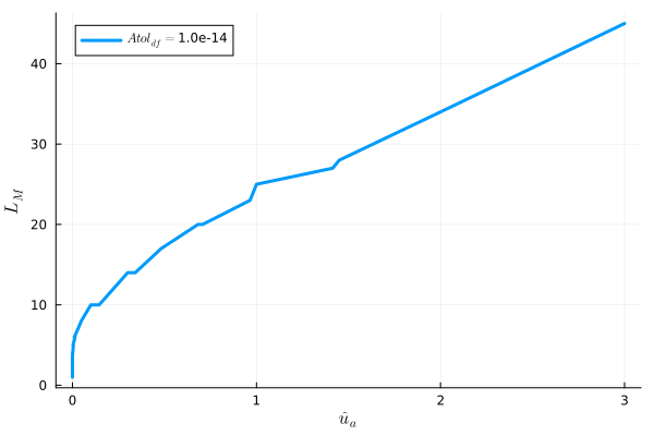
Figure 1: Convergence of SHE for drift-Maxwellian distribution: Truncated order $l_{M}$ as a function of $\hat{u}_{a}$ when tolerance $Atol_{df}=10^{-14}$.

III.3.1 Closure in $(l)$ space

For moderately anisotropic plasmasBell et al. (2006); Wang et al. (2025a), the series on the right side of the Eq. (6) will converge rapidly. Similar to Grad’s methodGrad (1949), the order $l$ can be truncated at a maximum value, $l_{M}$, where the subscript $M$ stands for $max$, satisfying that $\mathrm{max}|\hat{f}_{l}(\boldsymbol{r},v,t)|\leq Atol_{df}$ where $\hat{f}_{l}=v_{ath}^{3}n_{a}^{-1}f_{l}$. Here, $Atol_{df}$ is a tolerance with a default value of $10^{-14}$. Hence, $0\leq l\leq l_{M}$.

The convergence of SHE for drift-Maxwellian distribution is depicted in Fig. 1. It shows that the truncated order $l_{M}$ is a monotonic function of normalized average velocity, $\hat{u}_{a}=u_{a}/v_{ath}$. For example when $\hat{u}_{a}=3$ and $Atol_{df}=10^{-14}$, the maximum order, $l_{M}=45$. Moderately anisotropic plasmas can be defined as the system without significant asymmetric characteristics such as beam, where the truncated order $l_{M}\leq 45$ when tolerance $Atol_{df}=10^{-14}$. A more rigorous definition of anisotropy is provided in Sec. III.3.2 with the closure in $(j)$ space. Based on above definition, $l_{M}$ is typically not larger than $45$ for moderately anisotropic plasmas. This method is referred to as the natural truncation method in this article.

When applying the natural truncation method in the $(l)$ space and the truncated order $l_{M}$ is sufficiently large (maybe change with time), the amplitude functions with order larger than $l_{M}$ can simply be negligible. Subsequently, the higher-order kinetic moments with order $l\geq l_{M}+1$ in the KMEE (20) are negligible small quantities, that is

$$\mathcal{M}_{j,l}\left(\boldsymbol{r},t\right) \equiv 0,\quad\forall j,\quad l\geq l_{M}+1\leavevmode\nobreak\ .$$ (66)

This is the natural closure relation (NCR) in the $(l)$ space. Employing NCR, the KMEE represented by Eq. (28) with order $l_{M}\geq 1$ can be simplified to:

$$\frac{\partial}{\partial t}\mathcal{M}_{j,l_{M}}\left(\boldsymbol{r},t\right) = -C{{}_{A}}{{}_{l-1}}\frac{\partial}{\partial z}{\mathcal{M}}{{}_{j+1,l-1}}+C{{}_{E}}{{}_{j,l-1}}\frac{Z_{a}}{m_{a}}E_{z}{\mathcal{M}}{{}_{j-1,l-1}},\quad l=l_{M}\leavevmode\nobreak\ .$$ (67)

Notes that when $l=0$, $C{{}_{A}}{{}_{l-1}}=C{{}_{E}}{{}_{j,l-1}}=C{{}_{E}}{{}_{j,l-1}}\equiv 0$. Hence, KMEE (28) reduces to:

$$\frac{\partial}{\partial t}{\mathcal{M}}{{}_{j,0}}\left(\boldsymbol{r},t\right) = -C{{}_{A}}{{}_{l+1}}\frac{\partial}{\partial z}{\mathcal{M}}{{}_{j+1,l+1}}+C{{}_{E}}{{}_{j,l+1}}\frac{Z_{a}}{m_{a}}E_{z}{\mathcal{M}}{{}_{j-1,l+1}},\quad l=0\leavevmode\nobreak\ .$$ (68)

We can observe that the KMEE with order $(j,l=0)$ is independent of the kinetic moments with order $l-1$. That is to say that when $l_{M}=0$, applying NCR (66) results in:

$$\frac{\partial}{\partial t}{\mathcal{M}}{{}_{j,0}}\left(\boldsymbol{r},t\right) = 0,\quad\forall j\leavevmode\nobreak\ .$$ (69)

That is Eq. (29), representing the situation for collisionless plasmas when the velocity space exhibits spherical symmetry.

III.3.2 Closure in $(j)$ space

For moderately anisotropic plasmas, the FDIF hypothesisWang et al. (2025b, a) is an effective assumption to offer closure and capture the nonlinearity of the plasmas system. According to this hypothesis, we assume that the $l^{th}$-order amplitude distribution has distinguishable independent features with number $N_{l}$. Then, if we know the values of $N_{l}$ kinetic moments $\mathcal{M}_{j,l}$ with a collection of $(j)$, these features can be determined by these given kinetic moments. Here, we refer to the collection of $(j)$ as a vector, for example, $\boldsymbol{j}_{l}=[j_{m},\cdots,j-1,j,j+1,\cdots,j_{M}]$ where subscripts $m$ and $M$ stand for $min$ and $max$ respectively. Subsequently, $\mathcal{M}_{j\leq j_{m}-1,l}$ and $\mathcal{M}_{j\geq j_{M}+1,l}$ are dependent on kinetic moments within collection $\boldsymbol{j}_{l}$. Therefore, the closure relation in $(j)$ space can be expressed as:

$$\mathcal{M}_{j,l}\left(\boldsymbol{r},t\right) = \mathcal{M}_{j,l}\left(\mathcal{M}_{j_{m},l},\mathcal{M}_{j_{m}+1,l},\cdots,\mathcal{M}_{j_{M}-1,l},\mathcal{M}_{j_{M},l}\right),\quad j\notin\boldsymbol{j}_{l}\leavevmode\nobreak\ .$$ (70)

The concrete formula of above equation can be derived based on the FDIF hypothesis.

To capture the nonlinearity of the amplitude function $f_{l}$ (nature for general situation of fusion plasmas), a King function expansion (KFE) method is introduced in Ref.Wang et al. (2025b, a), which can be expressed as:

$$f_{l}\left(v/v_{ath},t\right) = \frac{2\pi}{\pi^{3/2}}\frac{n_{a}}{v_{ath}^{3}}\sum{{}_{s=1}^{N_{K_{a}}}}\left[\hat{n}_{a_{s,l}}\mathcal{K}_{l}\left(\hat{v};\hat{u}_{a_{s,l}},\hat{v}_{{ath}_{s,l}}\right)\right]\leavevmode\nobreak\ .$$ (71)

Here, $N_{K_{a}}\in\mathbb{N}^{+}$, which maybe vary with different $l$. The normalized speed coordinate, $\hat{v}=v/v_{ath}$. Symbols $\hat{n}_{a_{s,l}}$, $\hat{u}_{a_{s,l}}$ and $\hat{v}_{{ath}_{s,l}}$ represent the characteristic parameters of $s^{th}$ sub-distribution of $f_{l}$, respectively referred to as weight, group velocity and group thermal velocity. Generally, the characteristic parameters typically depend on $l$ in common scenarios. Function $\mathcal{K}_{l}$ denotes a new special function introduced in Ref.Wang et al. (2025a), which is associated with the first class of modified Bessel functions,

$$\mathcal{K}_{l}\left(\hat{v};\iota,\sigma\right) = \frac{(l+1/2)}{\sigma^{2}\sqrt{2\left|\iota\right|\hat{v}}}\left(\frac{\left|\iota\right|}{\iota}\right)^{l}\mathrm{e}^{-\sigma^{-2}\left(\hat{v}^{2}+\iota^{2}\right)}\mathrm{Besseli}\left(\frac{2l+1}{2},2\frac{\left|\iota\right|}{\sigma^{2}}\hat{v}\right)\leavevmode\nobreak\ .$$ (72)

Moreover, referenceWang et al. (2025a) has demonstrated that KFE is a moment convergent method. Here, Eq. (71) is referred to as the general King mixture model (GKMM) and the responding plasma state referred to as local sub-equilibriumWang (2024). Specially, when characteristic parameters are independent of $l$, the GKMM reduce to King mixture model (KMM) and the responding plasma state referred to as local quasi-equilibriumWang (2024); Wang et al. (2025a).

Substituting Eq. (71) into the definition of kinetic moment (19) gives the characteristic parameter equations (CPEs), namely:

$$\mathcal{M}_{j,l}\left(\boldsymbol{r},t\right)\ =\ {C_{M}}_{j}^{l}\rho_{a}\left(v_{ath}\right)^{j}\sum_{s=1}^{N_{K_{a}}}\hat{n}_{a_{s,l}}(\hat{v}_{{ath}_{s,l}})^{j}\left(\frac{\hat{u}_{a_{s,l}}}{\hat{v}_{{ath}_{s,l}}}\right)^{l}\left[1+\sum_{\gamma=1}^{(j-l)/2}C_{j,l}^{\gamma}\left(\frac{\hat{u}_{a_{s,l}}}{\hat{v}_{{ath}_{s,l}}}\right)^{2\gamma}\right],\ \forall l,$$ (73)

where $j\in\left\{(l+2j_{p}-2)|j_{p}\in\mathbb{N}^{+}\right\}$ and coefficients $C_{j,l}^{\gamma}$, ${C_{M}}_{j}^{l}$ are given by:

$$C_{j,l}^{\gamma} = 2^{\gamma}\frac{(2l+1)!!C_{\gamma}^{(j-l)/2}}{(2l+2\gamma+1)!!},\quad{C_{M}}_{j}^{l}\ =\ \frac{1}{2^{(j-l)/2}}\frac{(l+j+1)!!}{(2l-1)!!}\leavevmode\nobreak\ .$$ (74)

Symbol $C_{\gamma}^{(j-l)/2}$ is the binomial coefficient. Hence, given a specific collection $\boldsymbol{j}_{l}$ with number $N_{l}=3N_{K_{a}}$ and the values of the corresponding kinetic moments, the characteristic parameters can be determined by the well-posed CPEs (73). It is nature to offer the closure in $(j)$ space based on the CPEs, given by:

$$\frac{\mathcal{M}_{j,l}}{\rho_{a}\left(v_{ath}\right)^{j}} = {C_{M}}_{j}^{l}\sum_{s=1}^{N_{K_{a}}}\hat{n}_{a_{s,l}}(\hat{v}_{{ath}_{s,l}})^{j}\left(\frac{\hat{u}_{a_{s,l}}}{\hat{v}_{{ath}_{s,l}}}\right)^{l}\left[1+\sum_{\gamma=1}^{(j-l)/2}C_{j,l}^{\gamma}\left(\frac{\hat{u}_{a_{s,l}}}{\hat{v}_{{ath}_{s,l}}}\right)^{2\gamma}\right],\quad j\notin\boldsymbol{j}_{l}\leavevmode\nobreak\ .$$ (75)

Denote Eq. (75) as the characteristic closure relation (CCR) in the $(l)$ space.

The definition of anisotropy for plasmas can also be provided with the aid of characteristic parameters in KFE (71), which is associated with the group velocity of $f_{l}$. For species $a$, we define that anisotropy is equivalent to the maximum value of $\left|\hat{u}_{a_{s,l}}\right|/\hat{v}_{{ath}_{s,l}}$ for all the order $(s,l)$, and is denoted as:

$$\mathfrak{a}_{a}\left(\boldsymbol{r},t\right) = \mathrm{max}\left[\left({\left|\hat{u}_{a_{s,l}}\right|}/{\hat{v}_{{ath}_{s,l}}}\right)_{s\in[1.2.\cdots,N_{K_{a}}],l\in[0,1,2,\cdots,l_{M}]}\right]\leavevmode\nobreak\ .$$ (76)

It is evident that the anisotropy of a drift-Maxwellian plasmas will be:

$$\mathfrak{a}_{a}\left(\boldsymbol{r},t\right) = |u_{a}|/v_{ath}\leavevmode\nobreak\ .$$ (77)

In particular, anisotropy becomes zero when $u_{a}=0$, corresponding to the Maxwellian distribution, which is an isotropic part. Therefore, isotropy is naturally a special state of anisotropy.

With the definition of anisotropy, the weakly anisotropic plasmas will be defined as a system where the anisotropy $\mathfrak{a}_{a}\leq 0.1$, including the system in thermodynamic equilibrium state and near-equilibrium state. While the moderately anisotropic plasmas is defined as a system where anisotropy $\mathfrak{a}_{a}\leq 3$, encompassing the weakly anisotropic plasmas, and the so-called subsonic regions to low supersonic plasmas.

For moderately anisotropic plasmas, the proposed approach will be effective because of the fast convergence of SHE and KFE (complexity is determined by the kinetic effects of plasmas). However, if there are significant asymmetric characteristics in the plasmas system, such as a beam with $u_{a}/v_{ath}>3$ or some group velocity satisfies $\hat{u}_{a_{s,l}}/\hat{v}_{{ath}_{s,l}}>3$, the given framework in this study might become inefficient or even fail due to the slow convergence of SHE.

IV Conclusion

In this paper, we propose the transport theory derived from the 1D-2V Vlasov equation when velocity space exhibits axisymmetry, which is a kinetic moment-closed model (KMCM) for moderately anisotropic nonequilibrium plasmas. By utilizing the King function expansion (KFE) method which is based on the finitely distinguishable independent features (FDIF) hypothesis, the characteristic parameter equations (CPEs) are provided, serving as the closure relations of the transport equations. The presented model composed of the transport equations and closure relations, typically is a nonlinear system, which requires an optimization algorithm to solve numerically.

V Acknowledgments

References

- Vlasov (1968) A. A. Vlasov, Soviet Physics Uspekhi 10, 721 (1968).
- Mintzer (1965) D. Mintzer, Physics of Fluids 8, 1076 (1965).
- Schunk (1977) R. W. Schunk, Reviews of Geophysics 15, 429 (1977).
- Thomas et al. (2012) A. G. Thomas, M. Tzoufras, A. P. Robinson, R. J. Kingham, C. P. Ridgers, M. Sherlock, and A. R. Bell, Journal of Computational Physics 231, 1051 (2012).
- Wang et al. (2025a) Y. Wang, J. Xiao, Y. Zheng, Z. Zou, P. Zhang, and G. Zhuang, Journal of Computational Physics (Under review) (2025a), arXiv:2408.01616 [math.NA] .
- Grad (1949) H. Grad, Communications on Pure and Applied Mathematics 2, 331 (1949).
- Wang (2024) Y. Wang, (2024), arXiv:2409.12573 [physics.plasm-ph] .
- Chapman (1916) S. Chapman, Proceedings of the Royal Society of London. Series A, Containing Papers of a Mathematical and Physical Character 93, 1 (1916).
- Chapman and Cowling (1953) S. Chapman and T. G. Cowling, The Mathematical Theory of Non-Uniform Gases (Cambridge University Press, 1953).
- Burnett (1935) D. Burnett, Proceedings of the London Mathematical Society s2-39, 385 (1935).
- Wang et al. (2025b) Y. Wang, J. Xiao, X. Rao, P. Zhang, Y. Adil, and G. Zhuang, Chinese Physics B 1 (2025b).
- Wang et al. (2024) Y. Wang, S. Wu, and P. Fan, Chinese Physics B (Under review) (2024), arXiv:2409.10060 [physics.plasm-ph] .
- Min and Liu (2015) K. Min and K. Liu, Journal of Geophysical Research: Space Physics 120, 2739 (2015).
- Bell et al. (2006) A. R. Bell, A. P. Robinson, M. Sherlock, R. J. Kingham, and W. Rozmus, Plasma Physics and Controlled Fusion 48 (2006).
- Tzoufras et al. (2011) M. Tzoufras, A. R. Bell, P. A. Norreys, and F. S. Tsung, Journal of Computational Physics 230, 6475 (2011).
- Johnston (1960) T. W. Johnston, Physical Review 120, 1103 (1960).
- Arfken and Pan (1971) G. Arfken and Y. K. Pan, American Journal of Physics 39, 461 (1971).
- Freidberg (2014) J. P. Freidberg, Ideal MHD, Vol. 9781107006 (Cambridge University Press, 2014) pp. 1–722.