On principal eigenvalues of linear time-periodic parabolic systems: symmetric mutation case

Abstract.

The paper is concerned with the effect of the spatio-temporal heterogeneity on the principal eigenvalue of some linear time-periodic parabolic system. Various asymptotic behaviors of the principal eigenvalue and its monotonicity, as a function of the diffusion rate and frequency, are first derived. In particular, some singular behaviors of the principal eigenvalues are observed when both diffusion rate and frequency approach zero, with some scalar time-periodic Hamilton-Jacobi equation as the limiting equation. Furthermore, we completely classify the topological structures of the level sets for the principal eigenvalues in the plane of frequency and diffusion rate. Our results not only generalize most of the findings in [26] for scalar periodic-parabolic operators, but also reveal more rich global information, for time-periodic parabolic systems, on the dependence of the principal eigenvalues upon the spatio-temporal heterogeneity.

1. Introduction

Consider the coupled periodic-parabolic eigenvalue problem

(1.1) $$\left\{\begin{array}[]{ll}\vskip 6.0pt plus 2.0pt minus 2.0pt\omega\partial_{t}{\bm{\varphi}}-\rho{\bf D}\Delta{\bm{\varphi}}-{\bf A}(x,t){\bm{\varphi}}=\lambda{\bm{\varphi}}&\mathrm{in}~\Omega\times\mathbb{R},\\ \vskip 6.0pt plus 2.0pt minus 2.0pt\nabla{\bm{\varphi}}\cdot\nu=0&\mathrm{on}~\partial\Omega\times\mathbb{R},\\ {\bm{\varphi}}(x,t)={\bm{\varphi}}(x,t+1),&\mathrm{in}~\Omega\times\mathbb{R},\end{array}\right.$$

where $\Omega$ is a bounded domain in $\mathbb{R}^{n}$ with smooth boundary $\partial\Omega$ and $\nu(x)$ denotes the unit outward normal vector at $x\in\partial\Omega$. The operator $\Delta=\sum_{i=1}^{n}\partial_{x_{i}x_{i}}$ is the Laplace operator in $\mathbb{R}^{n}$ and ${\bf D}={\rm diag}(d_{1},\cdots,d_{n})$ is an $n\times n$ diagonal matrix with constant $d_{i}>0$, $i=1,\cdots,n$. For each $(x,t)\in\Omega\times\mathbb{R}$, ${\bf A}(x,t)$ is an essentially positive (cooperative) matrix (its off-diagonal entries are nonnegative), which is assumed to be symmetric and time-periodic with unit period. Inspired by [2, 36], we assume ${\bf A}=(a_{ij})_{n\times n}$ is fully coupled, i.e. the index set $\{1,\cdots,n\}$ cannot be split up in two disjoint nonempty sets $\mathcal{I}$ and $\mathcal{J}$ such that $a_{ij}(x,t)\equiv 0$ in $\Omega\times\mathbb{R}$ for $i\in\mathcal{I}$ and $j\in\mathcal{J}$. Parameters $\omega,\rho>0$ represent the frequency and diffusion rate, respectively.

By the Krein-Rutman theorem [21], it is shown in [2, 36] that problem (1.1) admits a real and simple eigenvalue, called principal eigenvalue. It has the smallest real part among all eigenvalues of (1.1) and corresponds to a positive eigenfunction, for which each entry is a positive time-periodic function. Our study is focused on the dependence of principal eigenvalue on frequency and diffusion rate.

1.1. Background and motivations

There has recently been considerable interest in issues related to qualitative analysis of the principal eigenvalue for problem (1.1); see for example [2, 5, 9, 23, 38]. Such interest stems mainly from the study of reaction-diffusion systems in spatio-temporally heterogeneous media. In particular, the principal eigenvalue can often be regarded as a threshold value in determining the dynamics of the associated nonlinear systems [3, 7, 17, 24].

Our motivation comes from the following linear system for $n$ phenotypes of a species with densities ${\bf u}(x,t)=(u_{1}(x,t),\cdots,u_{n}(x,t))$:

(1.2) $$\left\{\begin{array}[]{ll}\vskip 6.0pt plus 2.0pt minus 2.0pt\omega\partial_{t}{\bf u}=\rho{\bf D}\Delta{\bf u}+{\bf M}(x,t){\bf u}+{\rm diag}(c_{i}(x,t)){\bf u}&\mathrm{in}~\Omega\times(0,+\infty),\\ \nabla{\bf u}\cdot\nu=0&\mathrm{on}~\partial\Omega\times(0,+\infty),\end{array}\right.$$

where ${\rm diag}(c_{i}(x,t))$ is a diagonal matrix, with each $c_{i}$ being a time-periodic function denoting the birth-death rate of phenotype $i$. The essentially positive matrix function ${\bf M}(x,t)=(m_{ij}(x,t))_{n\times n}$ satisfying

$$m_{ii}(x,t)=-\sum_{j\not=i}m_{ij}(x,t),\quad\forall(x,t)\in\Omega\times\mathbb{R},\,\,i=1,\cdots,n,$$

represents the mutation of phenotypes.

The long-time behaviors of the solution to (1.2) is determined by the signs of the principal eigenvalue of problem (1.1) with

$${\bf A}(x,t)={\bf M}(x,t)+{\rm diag}(c_{i}(x,t)),\quad\forall(x,t)\in\Omega\times\mathbb{R}.$$

When ${\bf M}\equiv 0$, i.e. there is no mutation, problem (1.1) can be decoupled as the following $n$ scalar time-periodic parabolic problems:

(1.3) $$\begin{cases}\begin{array}[]{ll}\omega\partial_{t}\varphi-\rho d_{i}\Delta\varphi-c_{i}(x,t)\varphi=\lambda\varphi&\mathrm{in}~\Omega\times\mathbb{R},\,\,i=1,\cdots,n,\\ \nabla\varphi\cdot\nu=0&\mathrm{on}~\partial\Omega\times\mathbb{R},\\ \varphi(x,t)=\varphi(x,t+1)&\mathrm{in}~\Omega\times\mathbb{R},\end{array}\end{cases}$$

which admits the unique principal eigenvalue, denoted by $\lambda_{i}(\omega,\rho)$, for each $i=1,\cdots,n$; see [16, Proposition 16.1]. The outcomes of phenotypes in (1.2) are independent in this case, and phenotype $i$ is able to persist if and only if $\lambda_{i}(\omega,\rho)<0$. This motivates extensive researches on scalar problem (1.3) in order to clarify the effect of spatio-temporal heterogeneity on the persistence of phenotypes, mainly focusing on the asymptotic behaviors of $\lambda_{i}(\omega,\rho)$ with respect to frequency $\omega$ and diffusion rate $\rho$; see e.g. [16, 18, 26, 29, 33]. These findings turn out to have wide range of applications in studies of reaction-diffusion equations [3, 16, 17, 34].

A natural question is how the spatio-temporal heterogeneity may affect the dynamics of (1.2) when the mutation exists. We assume ${\bf M}$ is a time-periodic and fully coupled matrix function. In the simplest case, ${\bf M}$ is a discrete Laplacian, characterized as a symmetric and essentially positive constant matrix. Then all phenotypes will exhibit the same outcome and their persistence can be determined by the principal eigenvalue $\lambda(\omega,\rho)$ of coupled problem (1.1). To address the question, we are motivated to investigate the qualitative properties of $\lambda(\omega,\rho)$ as a function of $\omega$ and $\rho$. For technical reasons we specifically focus on the case of symmetric mutation, where matrix ${\bf M}$ (and thus ${\bf A}$) is assumed to be symmetric throughout this paper. We left the general cases for further studies.

When matrix ${\bf A}$ is independent of $x$ variable, problem (1.1) can be reduced to a time-periodic system in patchy environment [32, 35] and the corresponding principal eigenvalue is independent of the diffusion rate $\rho$. The monotonicity of principal eigenvalue with respect to frequency $\omega$ was established in [28] and subsequently applied in [22] to investigate the dispersal-induced growth phenomenon. We refer to [5, 20, 22] for details. In contrast, when matrix ${\bf A}$ is time-independent, problem (1.1) becomes a cooperative elliptic problem [36] and principal eigenvalue remains unaffected by frequency $\omega$. The asymptotic limits of principal eigenvalue as diffusion rate $\rho$ approaches zero was proved by Dancer [9] and was extended by Lam and Lou in [23] to more general cases, with applications to nonlinear competition population models.

When matrix ${\bf A}$ depends on both variables $x$ and $t$, much less is known about the dependence of principal eigenvalue on parameters. A few existing results can be found in [2, 15, 38], which generalized the results in [9, 23] and established the asymptotic behaviors of principal eigenvalue for small or large diffusion rate. Among others, the following result holds.

Theorem 1.1 ([2]).

Let $\lambda(\omega,\rho)$ be the principal eigenvalue of (1.1), then for each $\omega>0$,

$$\lim_{\rho\to 0}\lambda(\omega,\rho)=\underline{h}(\omega):=\min_{x\in\overline{\Omega}}h(x,\omega),$$

where for any $x\in\Omega$ and $\omega>0$, $h(x,\omega)$ denotes the principal eigenvalue of the problem

(1.4) $$\omega\frac{{\rm d}{\bm{\phi}}}{{\rm d}t}-{\bf A}(x,t){\bm{\phi}}=h{\bm{\phi}},\qquad{\bm{\phi}}(t)={\bm{\phi}}(t+1),\,\,\,\,t\in\mathbb{R}.$$

In the present paper, we will establish some monotonicity and asymptotic behaviors of the principal eigenvalue for problem (1.1). They lead to the complete classification for the topological structures of its level sets, as a function of frequency $\omega$ and diffusion rate $\rho$. This will help us better understand the combined effects of $\omega$ and $\rho$ on the principal eigenvalue.

1.2. Main results I: asymptotics and monotonicity

We define

(1.5) $$\underline{C}:=-\int_{0}^{1}\max_{x\in\overline{\Omega}}\mu({\bf A}(x,t)){\rm d}t\quad\text{and}\quad C_{*}:=-\max_{x\in\overline{\Omega}}\int_{0}^{1}\mu({\bf A}(x,t)){\rm d}t,$$

where $\mu({\bf A}(x,t))$ denotes the maximal eigenvalue of matrix ${\bf A}(x,t)$ associated with a nonnegative eigenvector. By Theorem 1.1 and [28, Theorem 2.1], it follows that

$$\lim_{\omega\to 0}\lim_{\rho\to 0}\lambda(\omega,\rho)=\lim_{\omega\to 0}\underline{h}(\omega)=C_{*}.$$

In contrast, Proposition 2.1 and [9, Theorem 1] imply that

$$\lim_{\rho\to 0}\lim_{\omega\to 0}\lambda(\omega,\rho)=\lim_{\rho\to 0}\underline{\lambda}(\rho)=\underline{C},$$

where $\underline{\lambda}(\rho)$ is defined in Proposition 2.1 to serve as the limit of $\lambda(\omega,\rho)$ as $\omega\to 0$. This implies that the double limit of $\lambda(\omega,\rho)$ as $(\omega,\rho)\to(0,0)$ does not exist once $\underline{C}\neq C_{*}$. This motivates us to consider the asymptotic behaviors of $\lambda(\omega,\rho)$ near $(\omega,\rho)=(0,0)$ and study the transition between the two regimes described above.

Theorem 1.2.

Let $\lambda(\omega,\rho)$ denote the principal eigenvalue of problem (1.1). Then

$$\lim_{(\omega,\rho)\to(0,0)\atop\frac{\omega}{\sqrt{\rho}}\to 0}\lambda(\omega,\rho)=\underline{C}\quad\text{and}\quad\lim_{(\omega,\rho)\to(0,0)\atop\frac{\omega}{\sqrt{\rho}}\to+\infty}\lambda(\omega,\rho)=C_{*}.$$

Furthermore, for any ${\bf p}\in\mathbb{R}^{n}$, let ${\rm H}({\bf p},x,t)\in\mathbb{R}$ be the maximal eigenvalue of matrix

$${\rm diag}\{d_{1}|{\bf p}|^{2},\cdots,d_{n}|{\bf p}|^{2}\}+{\bf A}(x,t)$$

associated with a nonnegative eigenvector. Then there holds

$$\lim_{(\omega,\rho)\to(0,0)\atop\frac{\omega}{\sqrt{\rho}}\to\vartheta}\lambda(\omega,\rho)=C(\vartheta),$$

whereas $C(\vartheta)$ is the unique value for which the following time-periodic Hamilton-Jacobi equation admits a Lipschitz viscosity solution:

(1.6) $$\begin{cases}\begin{array}[]{ll}\vartheta\partial_{t}U+{\rm H}(\nabla U,x,t)=-C(\vartheta)&\mathrm{in}~\Omega\times\mathbb{R},\\ \nabla U\cdot\nu=0&\mathrm{on}~\partial\Omega\times\mathbb{R},\\ U(x,t)=U(x,t+1)&\mathrm{in}~\Omega\times\mathbb{R}.\end{array}\end{cases}$$

Moreover, $C(\vartheta)$ is continuous in $\vartheta$, $C(\vartheta)\to\underline{C}$ as $\vartheta\to 0$, and $C(\vartheta)\to C_{*}$ as $\vartheta\to+\infty$.

Theorem 1.2 indicates that the transition of various asymptotic behaviors for principal eigenvalue $\lambda(\omega,\rho)$ in the regime $(\omega,\rho)\to(0,0)$ occurs at $\omega\approx\sqrt{\rho}$. This is connected by the time-periodic Hamilton-Jacobi equation (1.6) with some convex and coercive Hamiltonian that represents the maximal eigenvalue of some nonnegative matrix. It is somewhat interesting and surprising that the limiting behaviors of system (1.1) can be determined by a scalar Hamilton-Jacobi equation. This is a generalization of [26, Theorem 1.2] for periodic-parabolic operators and the proof is much more involved for the present case of systems.

The problem of identifying a pair $(C(\vartheta),U_{\vartheta})$ for which $U_{\vartheta}$ is a viscosity solution of (1.6) is known as an additive eigenvalue problem. This is related to weak KAM theory [19, 37] and homogenization theory [11, 31], both of which have extensive applications in the asymptotic propagation [6, 13] and the evolution of dispersal [25] for reaction diffusion equations. Problem (1.6) has a viscosity solution only if $C(\vartheta)$ is assigned a specific value, for which the uniqueness was established in the pioneering work [31]. Our next result is to provide more insight on the connections between the principal eigenvalue and such critical value.

Theorem 1.3.

Let $C(\omega/\sqrt{\rho})$ be the critical value of (1.6) with $\vartheta=\omega/\sqrt{\rho}$. Then $\lambda(\omega,\rho)\geq C(\omega/\sqrt{\rho})$ for all $\omega,\rho>0$. Moreover, the critical value $C(\vartheta)$ is non-decreasing in $\vartheta>0$.

The inequality in Theorem 1.3 is a reduced version of Theorem 4.2, in which more precise estimation is provided based on the associated eigenfunctions. The monotonicity in Theorem 1.3 is potentially of interest in understanding the effect of temporal heterogeneity on “effect Hamiltonians” as studied in [11, 12], where the asymptotic behaviors of $C(\vartheta)$ for more general time-periodic Hamiltonian in (1.6) are discussed.

A corollary of Theorem 1.3 is that $\lambda(\vartheta\sqrt{\rho},\rho)\geq C(\vartheta)$ for all $\rho,\vartheta>0$. In view of $\lambda(\vartheta\sqrt{\rho},\rho)\to C(\vartheta)$ as $\rho\to 0$ as shown in Theorem 1.2, this implies $\lambda(\vartheta\sqrt{\rho},\rho)$ attains its global minimal at $\rho=0$. A natural conjecture is that $\lambda(\vartheta\sqrt{\rho},\rho)$ is monotone increasing in $\rho$ for any $\vartheta>0$. The following result gives a positive answer.

Theorem 1.4.

Let $\lambda(\omega,\rho)$ denote the principal eigenvalue of (1.1). Suppose that $\rho=\rho(\omega)\in C^{1}((0,\infty))$, $\rho^{\prime}(\omega)\geq 0$, and $\left[\rho(\omega)/\omega^{2}\right]^{\prime}\leq 0$ in (1.1). Then $\lambda(\omega,\rho(\omega))$ is non-decreasing in $\omega$. In particular, for each fixed $\rho>0$, $\omega\mapsto\lambda(\omega,\rho)$ is non-decreasing.

Theorem 1.4 generalizes the results presented in [26, Theorem 1.1] for the scalar periodic-parabolic case and in [28, Theorem 1.1] for the spatially homogeneous case. Our proof offers a more straightforward and simplified approach in contrast to those in [26, 28], based on the equality provided in Lemma 4.1. The necessary and sufficient condition on the strict monotonicity is detailed in Theorem 4.3. We refer to [14] for a related result on the time-periodic nonlocal dispersal cooperative systems. However, the question of monotonicity in situations where matrix ${\bf A}$ is not necessarily symmetric remains open.

1.3. Main results II: level sets and applications

As applications of the above results, we are able to provide a complete classification of the level sets for principal eigenvalue of problem (1.1) as a function of frequency $\omega$ and diffusion rate $\rho$ in Theorem 5.4. It identifies five distinct types of topological structures for the level sets, which is a more intricate finding compared to the results in [26, Theorem 1.3] concerning the scalar time-periodic parabolic operators, where only two different topological structures were found. An interesting consequence of Theorem 5.4 is the implication on the non-monotone dependence of principal eigenvalue on the diffusion rate $\rho$ as shown in Corollary 5.5. This is in strong contrast to the time-independent scenario, wherein the principal eigenvalue is non-decreasing in $\rho$. To shorten the introduction, we move the materials for Theorem 5.4 to section 5 and refer to Fig. 3 for illustrations.

In what follows, we shall apply Theorem 5.4 to system (1.2) and characterize the parameter regions for the persistence and extinction of phenotypes. Assume the time-periodic mutation matrix ${\bf M}$ is essentially positive and fully coupled, then all phenotypes will interact with each other and the persistence of each phenotype is completely determined by the principal eigenvalue $\lambda(\omega,\rho)$ of system (1.1) with ${\bf A}={\bf M}+{\rm diag}(c_{i})$. In particular, the persistence region for problem (1.2) can be defined as

$$\mathbb{E}:=\{(\omega,\rho)\in\mathbb{R}_{+}^{2}:\,\,\lambda(\omega,\rho)<0\},$$

where $\mathbb{R}_{+}=(0,+\infty)$. This means that all phenotypes of the species will persist when $(\omega,\rho)\in\mathbb{E}$, whereas all phenotypes will become extinction when $(\omega,\rho)\not\in\mathbb{E}$. As a direct consequence of Theorem 5.4, the persistence region $\mathbb{E}$ can be characterized as follows.

Corollary 1.5.

Let $\underline{C}\leq C_{*}\leq\underline{C}^{+},C_{*}^{+}\leq\overline{C}$ be defined in (1.5) and (5.1) with ${\bf A}={\bf M}+{\rm diag}(c_{i})$ (see also Lemma 5.1). Then $\mathbb{E}=\emptyset$ if $\underline{C}\geq 0$, and $\mathbb{E}=\mathbb{R}_{+}^{2}$ if $\overline{C}\leq 0$. Otherwise, if $\underline{C}<0<\overline{C}$, then there exists uniquely a continuous function $\overline{\omega}:{\rm dom}(\overline{\omega})\mapsto(0,+\infty)$ such that

$$\mathbb{E}=\{(\omega,\rho)\in\mathbb{R}_{+}^{2}:\,\omega<\overline{\omega}(\rho),\,\,\,\rho\in{\rm dom}(\overline{\omega})\}.$$

The domain ${\rm dom}(\overline{\omega})$ and asymptotic behaviors of function $\overline{\omega}$ can be characterized as follows.

• If $\underline{C}<0<C_{*}$, then ${\rm dom}(\overline{\omega})=(0,\overline{\rho})$ for some $\overline{\rho}>0$, and

  $$\overline{\omega}(\rho)\to 0\quad\text{as }\,\,\rho\searrow 0\text{ and }\rho\nearrow\overline{\rho}.$$

• If $C_{*}<0<\min\{C_{*}^{+},\underline{C}^{+}\})$, then ${\rm dom}(\overline{\omega})=(0,\overline{\rho})$ for some $\overline{\rho}>0$, and

  $$\overline{\omega}(\rho)\to\underline{h}^{-1}(0)>0\text{ as }\rho\searrow 0\quad\text{ and }\quad\overline{\omega}(\rho)\to 0\text{ as }\rho\nearrow\overline{\rho}.$$

• If $C_{*}^{+}<0<\underline{C}^{+}$, then ${\rm dom}(\overline{\omega})=(\underline{\rho},\overline{\rho})$ for some $0<\underline{\rho}<\overline{\rho}$, and

  $$\overline{\omega}(\rho)\to+\infty\text{ as }\rho\searrow\underline{\rho}\quad\text{ and }\quad\overline{\omega}(\rho)\to 0\text{ as }\rho\nearrow\overline{\rho}.$$

• If $\underline{C}^{+}<0<C_{*}^{+}$,then ${\rm dom}(\overline{\omega})=(0,+\infty)$, and

  $$\overline{\omega}(\rho)\to\underline{h}^{-1}(0)>0\text{ as }\rho\searrow 0\quad\text{ and }\quad\overline{\omega}(\rho)\to\overline{h}^{-1}(0)>0\text{ as }\rho\nearrow+\infty.$$

• If $\max\{C_{*}^{+},\underline{C}^{+}\}<0<\overline{C}$, then ${\rm dom}(\overline{\omega})=(\underline{\rho},+\infty)$, and

  $$\overline{\omega}(\rho)\to+\infty\text{ as }\rho\searrow\underline{\rho}\quad\text{ and }\quad\overline{\omega}(\rho)\to\overline{h}^{-1}(0)>0\text{ as }\rho\nearrow+\infty.$$

Here functions $\underline{h}(\omega)$ and $\overline{h}(\omega)$ are defined in Theorem 1.1 and Proposition 2.2, respectively, both of which are non-decreasing and satisfy $\overline{h}^{-1}(0)<\underline{h}^{-1}(0)$.

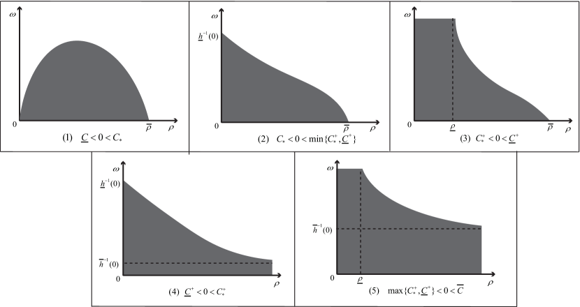
Figure 1. Illustrations of the persistence region $\mathbb{E}$ in the $\rho$-$\omega$ plane for the essentially positive and fully coupled mutation matrix ${\bf M}$, which is marked by the shaded areas, while the blank areas correspond to the region where $\lambda(\omega,\rho)\geq 0$.

Corollary 1.5 suggests that the persistence region $\mathbb{E}$ may exhibit five distinct types of topological structures in the $\rho$-$\omega$ plane, according to the combined effects of mutation matrix ${\bf M}$ and birth-death rate $c_{i}$. These structures are illustrated by the shaded areas in Fig. 1, which are separated with blank areas by the level set $\lambda(\omega,\rho)=0$ as characterized by Theorem 5.4. This in fact suggests much more complicated dynamics of (1.2) compared to the scenario where ${\bf M}\equiv 0$, indicating the absence of mutations in (1.2). Indeed, as aforementioned, when ${\bf M}\equiv 0$, phenotype $i$ can persist if and only if the principal eigenvalue $\lambda_{i}(\omega,\rho)$ for scalar problem (1.3) is of negative sign. According to the characterization of the level sets for $\lambda_{i}(\omega,\rho)$ in [26, Theorem 1.3], only two distinct types of topological structures, specifically types (1) and (3) in Fig. 1, are observed for the persistence region $\mathbb{E}$ under different conditions on the birth-death rate $c_{i}$. This finding suggests that our results in the present paper reveal some new phenomena, which cannot be observed from the decoupled system without mutations. Therefore, the analysis of the principal eigenvalue for system (1.1) can capture some intricate effects of mutations on the persistence of a species.

1.4. Organization of the paper

In section 2 we present some preliminary results on asymptotic behaviors of the principal eigenvalue for large/small frequency or diffusion rate. Section 3 is devoted to the asymptotic analysis of the principal eigenvalue near the origin and establishing Theorem 1.2. The monotone dependence of the principal eigenvalue is studied in section 4, where Theorems 1.3 and 1.4 are proved. Finally, in section 5 we classify the topological structures of level sets for the principal eigenvalue and establish some non-monotone dependence of principal eigenvalue on diffusion rate.

2. Preliminaries

In this section, we prepare some asymptotic behaviors of principal eigenvalue for problem (1.1), which generalize some results on the scalar time-periodic parabolic eigenvalue problems as studied in [17, 18, 29, 33]. Throughout the paper, for each $(x,t)\in\overline{\Omega}\times\mathbb{R}$, we assume ${\bf A}(x,t)=(a_{ij}(x,t))_{n\times n}$ is a symmetric and essentially positive matrix, with each $a_{ij}\in C(\overline{\Omega}\times\mathbb{R})$ being a time-periodic function with unit period.

The symmetric assumption on matrix ${\bf A}$ is not necessary throughout this section.

Proposition 2.1.

Let $\lambda(\omega,\rho)$ be the principal eigenvalue of problem (1.1). Then

• $\lambda(\omega,\rho)\to\overline{\lambda}(\rho)$ as $\omega\to+\infty$, where $\overline{\lambda}(\rho)$ denotes the principal eigenvalue of

  (2.1) $$-\rho{\bf D}\Delta{\bm{\phi}}-\widehat{\bf A}(x){\bm{\phi}}=\lambda{\bm{\phi}}\,\,\,\,\mathrm{in}~\,\,\,\Omega,\qquad\nabla{\bm{\phi}}\cdot\nu=0~~\mathrm{on}\,\,\,~\partial\Omega,$$

  with $\widehat{\bf A}$ being the temporally averaged matrix with entries $(\widehat{\bf A})_{ij}(x)=\int_{0}^{1}a_{ij}(x,t){\rm d}t$.

• $\lambda(\omega,\rho)\to\underline{\lambda}(\rho):=\int_{0}^{1}\lambda_{0}(t,\rho){\rm d}t$ as $\omega\to 0$, where for any $\rho>0$ and $t\in\mathbb{R}$, $\lambda_{0}(t,\rho)$ denotes the principal eigenvalue of the elliptic eigenvalue problem

  (2.2) $$-\rho{\bf D}\Delta{\bm{\phi}}-{\bf A}(x,t){\bm{\phi}}=\lambda{\bm{\phi}}\,\,\,\,\mathrm{in}~\,\,\,\Omega,\qquad\nabla{\bm{\phi}}\cdot\nu=0~~\mathrm{on}\,\,\,~\partial\Omega.$$

Proof.

Step 1. We first prove part (i). The proof can follow by the ideas in [33, Lemma 3.10] concerning scalar space-time periodic eigenvalue problems. We present the details for completeness. Let ${\bm{\varphi}}=(\varphi_{1},\cdots,\varphi_{n})>0$ be the principal eigenfunction of (1.1) associated with $\lambda(\omega,\rho)$, which can be normalized by $\sum_{i=1}^{n}\int_{0}^{1}\!\int_{\Omega}\varphi^{2}_{i}=1$. Recall that ${\bf A}(x,t)=(a_{ij}(x,t))_{n\times n}$ with $1$-periodic function $a_{ij}\in C(\Omega\times\mathbb{R})$. Multiplying both sides of (1.1) by $\varphi_{i}$ and integrating the resulting equation over $\Omega\times(0,1)$, we have

$$\rho\sum_{i=1}^{n}d_{i}\int_{0}^{1}\!\!\!\int_{\Omega}|\nabla\varphi_{i}|^{2}=\lambda(\omega,\rho)+\sum_{i,j=1}^{n}\int_{0}^{1}\!\!\!\int_{\Omega}a_{ij}\varphi_{i}\varphi_{j}.$$

Hence, by the uniform boundedness of $\lambda(\omega,\rho)$ we derive that

(2.3) $$\sum_{i=1}^{n}\int_{0}^{1}\!\!\!\int_{\Omega}|\nabla\varphi_{i}|^{2}\leq M/\rho,\quad\forall\omega,\rho>0.$$

Hereafter $M$ denotes some positive constant, which may vary from line to line but is always independent of $\omega$ and $\rho$. We next multiply both sides of (1.1) by $\partial_{t}\varphi_{i}$ and integrate the resulting equation over $\Omega\times(0,1)$, then

$$\omega\sum_{i=1}^{n}\int_{0}^{1}\!\!\!\int_{\Omega}|\partial_{t}\varphi_{i}|^{2}=-\frac{\rho}{2}\sum_{i=1}^{n}d_{i}\int_{0}^{1}\!\!\!\int_{\Omega}\partial_{t}(|\nabla\varphi_{i}|^{2})+\sum_{i,j=1}^{n}\int_{0}^{1}\!\!\!\int_{\Omega}a_{ij}\varphi_{j}\partial_{t}\varphi_{i}=\sum_{i,j=1}^{n}\int_{0}^{1}\!\!\!\int_{\Omega}a_{ij}\varphi_{j}\partial_{t}\varphi_{i},$$

which yields the following estimate

(2.4) $$\sum_{i=1}^{n}\int_{0}^{1}\!\!\!\int_{\Omega}|\partial_{t}\varphi_{i}|^{2}\leq M/\omega,\quad\forall\omega,\rho>0.$$

Combining (2.3) and (2.4), we observe that for each $i=1,\cdots,n$, function $\varphi_{i}$ is bounded in $H^{1}(\Omega\times(0,1))$ and $\partial_{t}\varphi_{i}\to 0$ in $L^{2}(\Omega\times(0,1))$ as $\omega\to+\infty$. Hence, by passing to a subsequence if necessary, we may assume that $\varphi_{i}\to\phi_{i}$ strongly in $L^{2}(\Omega\times(0,1))$ and weakly in $H^{1}(\Omega\times(0,1))$ for some $\phi_{i}\in H^{1}(\Omega\times(0,1))$ satisfying $\sum_{i=1}^{n}\int_{0}^{1}\!\!\int_{\Omega}\phi^{2}_{i}=1$. Then it follows by (2.4) that

$$\sum_{i=1}^{n}\int_{0}^{1}\!\!\!\int_{\Omega}|\partial_{t}\phi_{i}|^{2}\leq\liminf_{\omega\to 0}\sum_{i=1}^{n}\int_{0}^{1}\!\!\!\int_{\Omega}|\partial_{t}\varphi_{i}|^{2}=0,$$

and thus $\phi_{i}=\phi_{i}(x)$ is independent of $t$ variable.

Assume that $\lambda(\omega,\rho)\to\overline{\lambda}(\rho)$ for some $\overline{\lambda}(\rho)\in\mathbb{R}$ as $\omega\to+\infty$ by passing to a subsequence if necessary. It suffices to show that $\overline{\lambda}(\rho)$ is the principal eigenvalue of (2.1). To this end, multiply both sides of (1.1) by any test function in $H^{1}(\Omega\times(0,1))$ and let $\omega\to+\infty$ in the resulting equation, then we see that ${\bm{\phi}}=(\phi_{1},\cdots,\phi_{n})$ is a weak solution of the equation

(2.5) $$-\rho{\bf D}\Delta{\bm{\phi}}-{\bf A}(x,t){\bm{\phi}}=\overline{\lambda}(\rho){\bm{\phi}},\quad\,\,\forall(x,t)\in\Omega\times\mathbb{R}.$$

Due to ${\bm{\phi}}={\bm{\phi}}(x)$ is independent of $t$, we integrate (2.5) with respect to $t$ over $(0,1)$, then

$$-\rho{\bf D}\Delta{\bm{\phi}}-\widehat{\bf A}(x){\bm{\phi}}=\overline{\lambda}(\rho){\bm{\phi}},\quad\,\,\forall(x,t)\in\Omega\times\mathbb{R}.$$

In view of ${\bm{\phi}}>0$, by the uniqueness of principal eigenvalue of problem (2.1), we conclude the desired result. Step 1 is complete.

Step 2. We prove part (ii). For each $t\in\mathbb{R}$, denote by ${\bm{\phi}}=(\phi_{1},\cdots,\phi_{n})>0$ the principal eigenfunction of (2.2) corresponding to principal eigenvalue $\lambda_{0}(t,\rho)$. Set

$$\underline{\bm{\varphi}}(x,t):=\exp\left\{\frac{1}{\omega}\left(\underline{\lambda}(\rho)t-\int_{0}^{t}\lambda_{0}(s,\rho){\rm d}s\right)\right\}{\bm{\phi}}(x,t),$$

which is positive and $1$-periodic in $t$. Set $\underline{\bm{\varphi}}:=(\underline{\varphi}_{1},\cdots,\underline{\varphi}_{n})$ for $1$-periodic function $\underline{\varphi}_{i}\in C^{2,1}(\Omega\times\mathbb{R})$. By (2.2), direct calculations yield $\nabla\underline{\varphi}_{i}\cdot\nu=\underline{\varphi}_{i}\nabla\log\phi_{i}\cdot\nu=0$ for all $x\in\partial\Omega$ and

$$\omega\partial_{t}\underline{\varphi}_{i}-\rho d_{i}\Delta\underline{\varphi}_{i}-\sum_{j=1}^{n}a_{ij}\underline{\varphi}_{j}$$

$$= \Big{[}\underline{\lambda}(\rho)-\lambda_{0}(t,\rho)+\omega\frac{\partial_{t}\phi_{i}}{\phi_{i}}-\rho d_{i}\frac{\Delta\phi_{i}}{\phi_{i}}-\sum_{j=1}^{n}a_{ij}\frac{\phi_{j}}{\phi_{i}}\Big{]}\underline{\varphi}_{i}$$

$$= \left(\underline{\lambda}(\rho)+\omega\partial_{t}\log\phi_{i}\right)\underline{\varphi}_{i},\qquad\forall(x,t)\in\Omega\times\mathbb{R},\,\,\,i=1,\cdots,n.$$

Hence, for any given $\epsilon>0$, we can choose $\omega$ small such that

(2.6) $$\left\{\begin{array}[]{ll}\vskip 6.0pt plus 2.0pt minus 2.0pt\omega\partial_{t}\underline{\bm{\varphi}}-\rho{\bf D}\Delta\underline{\bm{\varphi}}-{\bf A}\underline{\bm{\varphi}}\leq(\underline{\lambda}(\rho)+\epsilon)\underline{\bm{\varphi}}&\mathrm{in}~\Omega\times\mathbb{R},\\ \vskip 6.0pt plus 2.0pt minus 2.0pt\omega\partial_{t}\underline{\bm{\varphi}}-\rho{\bf D}\Delta\underline{\bm{\varphi}}-{\bf A}\underline{\bm{\varphi}}\geq(\underline{\lambda}(\rho)-\epsilon)\underline{\bm{\varphi}}&\mathrm{in}~\Omega\times\mathbb{R},\\ \vskip 6.0pt plus 2.0pt minus 2.0pt\nabla\underline{\bm{\varphi}}\cdot\nu=0&\mathrm{on}~\partial\Omega\times\mathbb{R},\\ \underline{\bm{\varphi}}(x,t)=\underline{\bm{\varphi}}(x,t+1),&\mathrm{in}~\Omega\times\mathbb{R}.\end{array}\right.$$

Then we apply the comparison principle established by [2, section 2] to (2.6) and obtain

$$\underline{\lambda}(\rho)-\epsilon\leq\liminf_{\omega\rightarrow 0}\lambda(\omega,\rho)\leq\limsup_{\omega\rightarrow 0}\lambda(\omega,\rho)\leq\underline{\lambda}(\rho)+\epsilon,$$

which proves part (ii) by letting $\epsilon\to 0$. The proof is complete. ∎

As a complement to Theorem 1.1, we next consider the asymptotic behavior of principal eigenvalue $\lambda(\omega,\rho)$ for large diffusion rate $\rho$.

Proposition 2.2.

For each $\omega>0$, let $\overline{h}(\omega)$ be the principal eigenvalue of the problem

(2.7) $$\omega\frac{{\rm d}{\bm{\phi}}}{{\rm d}t}-\overline{\bf A}(t){\bm{\phi}}=h{\bm{\phi}},\qquad{\bm{\phi}}(t)={\bm{\phi}}(t+1),\,\,\,\,t\in\mathbb{R},$$

where $\overline{\bf A}$ is the spatially averaged matrix with entries $(\overline{\bf A})_{ij}(t)=\frac{1}{|\Omega|}\int_{\Omega}a_{ij}(x,t){\rm d}x$. Then

$$\lim_{\rho\to+\infty}\lambda(\omega,\rho)=\overline{h}(\omega).$$

Moreover, if the off-diagonal entries of ${\bf A}$ are independent of $x$ variable, then $\lambda(\omega,\rho)\leq\overline{h}(\omega)$ for all $\omega,\rho>0$, i.e. $\lambda(\omega,\rho)$ attains its global maximal at $\rho=+\infty$ for each $\omega>0$.

Proof.

Step 1. We first establish the limit of $\lambda(\omega,\rho)$ as $\rho\to+\infty$. Let ${\bm{\varphi}}=(\varphi_{1},\cdots,\varphi_{n})>0$, normalized by $\sum_{i=1}^{n}\int_{0}^{1}\!\int_{\Omega}\varphi^{2}_{i}=1$, be the principal eigenfunction of problem (1.1). Set

(2.8) $$f_{i}(x,t):=\varphi_{i}(x,t)-\frac{1}{|\Omega|}\int_{\Omega}\varphi_{i}(x,t){\rm d}x,\qquad i=1,\cdots,n.$$

Then $\int_{\Omega}f_{i}(x,t){\rm d}x=0$ for all $t\in\mathbb{R}$ and $1\leq i\leq n$. By the Poincaré’s inequality, there exists some constant $M>0$ depending only on $\Omega$ such that $\int_{\Omega}f_{i}^{2}\leq M\int_{\Omega}|\nabla f_{i}|^{2}$. Note from (2.8) that $\nabla f_{i}=\nabla\varphi_{i}$, whence by (2.3) we derive that

(2.9) $$\sum_{i=1}^{n}\int_{0}^{1}\!\!\!\int_{\Omega}f_{i}^{2}\leq M/\rho,\qquad i=1,\cdots,n.$$

Integrate (1.1) over $\Omega$ and substitute $\varphi_{i}=f_{i}+\frac{1}{|\Omega|}\int_{\Omega}\varphi_{i}$ into the resulting equation, then

(2.10) $$\omega\partial_{t}\int_{\Omega}\varphi_{i}-\sum_{j=1}^{n}(\overline{\bf A})_{ij}(t)\int_{\Omega}\varphi_{j}=\lambda(\omega,\rho)\int_{\Omega}\varphi_{i}+\sum_{j=1}^{n}\int_{\Omega}a_{ij}f_{j},\quad i=1,\cdots,n.$$

Multiplying both sides of (2.10) by $\int_{\Omega}\varphi_{i}$ and summing over index $i$ from $1$ to $n$, then by (2.9) and the boundedness of matrix $\overline{\bf A}$, we derive that

(2.11) $$\frac{\omega}{2}\partial_{t}\left[\sum_{i=1}^{n}(\int_{\Omega}\varphi_{i})^{2}\right]\leq(M+\lambda(\omega,\rho))\sum_{i=1}^{n}(\int_{\Omega}\varphi_{i})^{2}+O(\rho).$$

The adjoint problem of (2.7) can be written as

(2.12) $$-\omega\frac{{\rm d}{\bm{\phi}}}{{\rm d}t}-\overline{\bf A}(t){\bm{\phi}}=h{\bm{\phi}},\qquad{\bm{\phi}}(t)={\bm{\phi}}(t+1),\,\,\,\,t\in\mathbb{R}.$$

Denote by ${\bm{\phi}}(t)=(\phi_{1}(t),\cdots,\phi_{n}(t))>0$ the principal eigenfunction of (2.12) corresponding to $\overline{h}(\omega)$. Then multiplying both sides of (2.10) by ${\bm{\phi}}$ and integrating the resulting equation over $(0,1)$ yield

(2.13) $$(\overline{h}(\omega)-\lambda(\omega,\rho))\sum_{i=1}^{n}\int_{0}^{1}\left[\phi_{i}(t)\int_{\Omega}\varphi_{i}(x,t){\rm d}x\right]{\rm d}t=\sum_{i,j=1}^{n}\int_{0}^{1}\left[\phi_{i}(t)\int_{\Omega}a_{ij}f_{j}\right]{\rm d}t.$$

Hence, by (2.9) we have either $\lambda(\omega,\rho)\to\overline{h}(\omega)$ or $\int_{\Omega}\varphi_{i}(x,t){\rm d}x\to 0$ in $L^{1}((0,1))$ as $\rho\to+\infty$. The former completes the proof. It suffices to show that the latter is impossible.

Suppose it holds, then we can derive from (2.11) that $\int_{\Omega}\varphi_{i}(x,t){\rm d}x\to 0$ uniformly in $[0,1]$ as $\rho\to+\infty$. This together with (2.8) and (2.9) implies that

$$\lim_{\rho\to+\infty}\int_{0}^{1}\!\!\!\int_{\Omega}\varphi^{2}_{i}=0,\qquad i=1,\cdots,n.$$

This contradicts the normalization of ${\bm{\varphi}}$, so that the latter cannot hold. Hence, $\lambda(\omega,\rho)\to\overline{h}(\omega)$ as $\rho\to+\infty$, which completes the proof.

Step 2. We assume that the off-diagonal entries of ${\bf A}$ are independent of $x$ and show $\lambda(\omega,\rho)\leq\overline{h}(\omega)$ for all $\omega,\rho>0$. Recall that ${\bm{\varphi}}=(\varphi_{1},\cdots,\varphi_{n})>0$ is the principal eigenfunction of (1.1) associated to $\lambda(\omega,\rho)$. Inspired by [18], we define

$$w_{i}(t):=\exp\left(\frac{1}{|\Omega|}\int_{\Omega}\log\varphi_{i}(x,t){\rm d}x\right),\quad i=1,\cdots,n.$$

Recall ${\bf A}(x,t)=(a_{ij}(x,t))_{n\times n}$. By our assumption, $a_{ij}=a_{ij}(t)$ is independent of $x$ for all $i\neq j$. By (1.1), direct calculations yield

$$\omega\frac{{\rm d}\log w_{i}}{{\rm d}t}= \frac{1}{|\Omega|}\int_{\Omega}\frac{\omega\partial_{t}\varphi_{i}}{\varphi_{i}}{\rm d}x$$

$$= \lambda(\omega,\rho)+\frac{\rho d_{i}}{|\Omega|}\int_{\Omega}\frac{\Delta\varphi_{i}}{\varphi_{i}}{\rm d}x+\frac{1}{|\Omega|}\sum_{j=1}^{n}\int_{\Omega}\frac{a_{ij}\varphi_{j}}{\varphi_{i}}{\rm d}x$$

(2.14) $$= \lambda(\omega,\rho)+\frac{\rho d_{i}}{|\Omega|}\int_{\Omega}\frac{|\nabla\varphi_{i}|^{2}}{\varphi_{i}^{2}}{\rm d}x+\frac{1}{|\Omega|}\sum_{j=1}^{n}\int_{\Omega}\frac{a_{ij}\varphi_{j}}{\varphi_{i}}{\rm d}x$$

$$\geq \lambda(\omega,\rho)+\frac{1}{|\Omega|}\sum_{j=1}^{n}\int_{\Omega}\frac{a_{ij}\varphi_{j}}{\varphi_{i}}{\rm d}x.$$

By the definition of spatially averaged matrix $\overline{\bf A}$, using the Jensen’s inequality one has

$$\frac{1}{|\Omega|}\sum_{j=1}^{n}\int_{\Omega}\frac{a_{ij}\varphi_{j}}{\varphi_{i}}{\rm d}x =(\overline{\bf A})_{ii}+\frac{1}{|\Omega|}\sum_{j\neq i}a_{ij}(t)\int_{\Omega}\frac{\varphi_{j}}{\varphi_{i}}{\rm d}x$$

$$=(\overline{\bf A})_{ii}+\frac{1}{|\Omega|}\sum_{j\neq i}a_{ij}(t)\int_{\Omega}\exp(\log\varphi_{j}-\log\varphi_{i}){\rm d}x$$

$$\geq(\overline{\bf A})_{ii}+\sum_{j\neq i}a_{ij}(t)\exp\left[\frac{1}{|\Omega|}\int_{\Omega}\log\varphi_{j}{\rm d}x-\frac{1}{|\Omega|}\int_{\Omega}\log\varphi_{i}{\rm d}x\right]$$

$$=\sum_{j=1}^{n}\frac{(\overline{\bf A})_{ij}w_{j}}{w_{i}}.$$

This together with (2) gives

$$\omega\frac{{\rm d}w_{i}}{{\rm d}t}-\sum_{j=1}^{n}(\overline{\bf A})_{ij}w_{j}\geq\lambda(\omega,\rho)w_{i}\quad\text{ for }\,\,t\in\mathbb{R},\,\,\,i=1,\cdots,n,$$

and thus ${\bf w}=(w_{1},\cdots,w_{n})$ is a super-solution of problem (2.7). By comparison (see Proposition 2.4 of [2]), we derive $\lambda(\omega,\rho)\leq{\overline{h}}(\omega)$ for all $\omega>0$. The proof is complete. ∎

We conclude this section by stating a direct corollary of Proposition 2.2.

Corollary 2.3.

Let ${\bf B}(x)=(b_{ij}(x))_{n\times n}$ be any essentially positive and irreducible time-independent matrix. For any $\rho>0$, let $\lambda(\rho)$ be the principal eigenvalue of the elliptic problem

(2.15) $$-\rho{\bf D}\Delta{\bm{\varphi}}-{\bf B}(x){\bm{\varphi}}=\lambda{\bm{\varphi}}\,\text{ in }\,\Omega,\quad\nabla{\bm{\varphi}}\cdot\nu=0\,\text{ on }\,\partial\Omega.$$

Then $\lambda(\rho)\to\mu(\overline{\bf B})$ as $\rho\to+\infty$, where $\overline{\bf B}$ is the matrix with entries $(\overline{\bf B})_{ij}=\frac{1}{|\Omega|}\int_{\Omega}b_{ij}(x){\rm d}x$.

Proof.

Let ${\bf A}={\bf B}(x)$ be independent of $t$ in (1.1), then problem (1.1) is equivalent to (2.15). Hence, Corollary 2.3 is a direct consequence of Proposition 2.2. ∎

3. Asymptotic analysis near the origin

In this section, we are concerned with the asymptotic behaviors of the principal eigenvalue when both diffusion rate and frequency approach to zero and establish Theorem 1.2. To this end, we first consider the following asymptotic regime.

Proposition 3.1.

Let $\lambda(\omega,\rho)$ denote the principal eigenvalue of (1.1). Then

$$\lim_{(\omega,\rho)\to(0,0)\atop\frac{\omega}{\sqrt{\rho}}\to+\infty}\lambda(\omega,\rho)=C_{*}=-\max_{x\in\overline{\Omega}}\int_{0}^{1}\mu({\bf A}(x,t)){\rm d}t.$$

Proof.

Define ${\bm{\varphi}}=(\varphi_{1},\cdots,\varphi_{n})>0$, normalized by $\max_{1\leq i\leq n}\max_{\overline{\Omega}\times\mathbb{R}}\varphi_{i}=1$, as the principal eigenvector of (1.1) corresponding to $\lambda(\omega,\rho)$. Set

$$W_{i}(x,t;\omega,\rho):=-\sqrt{\rho}\log\varphi_{i}\left(x,\frac{\omega t}{\sqrt{\rho}}\right)\quad\text{ for all }(x,t)\in\Omega\times\mathbb{R},\,\,1\leq i\leq n.$$

Then $\min_{1\leq i\leq n}\min_{\overline{\Omega}\times\mathbb{R}}W_{i}(x,t;\omega,\rho)=0$ for all $\omega,\rho>0$. By (1.1), direct calculations yield that for any $1\leq i\leq n$,

(3.1) $$\begin{cases}\begin{array}[]{ll}\partial_{t}W_{i}-\sqrt{\rho}d_{i}\Delta W_{i}+d_{i}|\nabla W_{i}|^{2}+\displaystyle\sum_{j=1}^{n}a_{ij}(x,\tfrac{\omega t}{\sqrt{\rho}})e^{\frac{W_{i}-W_{j}}{\sqrt{\rho}}}=-\lambda(\omega,\rho)&\text{in }\,\,\Omega\times\mathbb{R},\\ \nabla W_{i}\cdot\nu=0&\text{on }\,\partial\Omega\times\mathbb{R}.\end{array}\end{cases}$$

Note that $\lambda(\omega,\rho)$ is uniformly bounded for all $\omega,\rho>0$ (see also Lemma 5.2). By the same arguments as in [13, Lemma 2.1], we may construct suitable super-solutions and apply the comparison principle to derive that

(3.2) $$\max_{1\leq i\leq n}\max_{\overline{\Omega}\times\mathbb{R}}|W_{i}(x,t;\omega,\rho)|\leq C,\,\,\quad\forall\rho>0,\,\,\forall\omega/\sqrt{\rho}\geq 1$$

for some constant $C$ independent of $\omega$ and $\rho$. Given any sequences $\{\omega_{k}\}_{k=1}^{\infty}$ and $\{\rho_{k}\}_{k=1}^{\infty}$ such that $\omega_{k},\rho_{k}\to 0$ and $\omega_{k}/\sqrt{\rho_{k}}\to+\infty$ as $k\to+\infty$, we assume $\lambda(\omega_{k},\rho_{k})\to\lambda_{\infty}$ for some $\lambda_{\infty}\in\mathbb{R}$. By the arbitrariness of $\{\omega_{k}\}_{k=1}^{\infty}$ and $\{\rho_{k}\}_{k=1}^{\infty}$, it suffices to show $\lambda_{\infty}=C_{*}$. The proof is separated into the following two steps.

Step 1. We prove $\lambda_{\infty}\geq C_{*}$. Define the following half-relaxed limit as in [4, Sect. 6]:

$$U_{i}(x,t):=\liminf_{k\to+\infty\atop(x^{\prime},t^{\prime})\to(x,t)}W_{i}(x^{\prime},t^{\prime};\omega_{k},\rho_{k})\quad\text{and}\quad U_{*}(x,t):=\min_{1\leq i\leq n}U_{i}(x,t),$$

which is well-defined due to (3.2). Clearly, $U_{*}$ is lower semi-continuous.

Set $\overline{d}=\max_{1\leq i\leq n}d_{i}>0$. We shall prove that $U_{*}$ is a lower semi-continuous viscosity super-solution of the Hamilton-Jacobi problem

(3.3) $$\begin{cases}\begin{array}[]{ll}\vskip 3.0pt plus 1.0pt minus 1.0pt\partial_{t}U_{*}+\overline{d}|\nabla U_{*}|^{2}+\int_{0}^{1}\mu({\bf A}(x,t)){\rm d}t=-\lambda_{\infty}&\text{in }\,\,\Omega\times\mathbb{R},\\ \nabla U_{*}\cdot\nu=0&\text{on }\,\partial\Omega\times\mathbb{R},\end{array}\end{cases}$$

where the boundary condition is understood in the viscosity sense [30]. Then we can apply the same arguments as in the proof of [26, Lemma 3.3] to derive that

$$\lambda_{\infty}\geq-\max_{x\in\overline{\Omega}}\int_{0}^{1}\mu({\bf A}(x,t)){\rm d}t=C_{*}.$$

To this end, we fix any smooth test function $\phi$ and assume that $U_{*}-\phi$ has a strict minimum at a point $(x_{0},t_{0})\in\overline{\Omega}\times\mathbb{R}$. By the definition of viscosity super-solution [19, 30], we must verify that at $(x_{0},t_{0})$, it holds

(3.4) $$\left\{\begin{array}[]{ll}\vskip 6.0pt plus 2.0pt minus 2.0pt\partial_{t}\phi+\overline{d}|\nabla\phi|^{2}+\int_{0}^{1}\mu({\bf A}(x_{0},t)){\rm d}t\geq-\lambda_{\infty}&\text{if }\,\,x_{0}\in\Omega,\\ \max\left\{\nabla\phi\cdot\nu,\,\,\partial_{t}\phi+\overline{d}|\nabla\phi|^{2}-\int_{0}^{1}\mu({\bf A}(x_{0},t)){\rm d}t+\lambda_{\infty}\right\}\geq 0&\text{if }\,\,x_{0}\in\partial\Omega.\end{array}\right.$$

Indeed, let ${\bf v}=(v_{1},\cdots,v_{n})>0$ denote the principal eigenvector of ${\bf A}(x,t)$ corresponding to the maximal eigenvalue $\mu({\bf A}(x,t))$, that is

(3.5) $$\sum_{j=1}^{n}a_{ij}(x,t)v_{j}=\mu({\bf A}(x,t))v_{i}\quad\text{ for all }(x,t)\in\Omega\times\mathbb{R},\,\,i=1,\cdots,n.$$

For any $1\leq i\leq n$ and $k\geq 1$, we define

(3.6) $$\begin{split}N_{i}(x,t;\omega_{k},\rho_{k}):=&\sqrt{\rho_{k}}\log v_{i}\left(x,\frac{\omega_{k}t}{\sqrt{\rho_{k}}}\right)\\ &-\frac{\sqrt{\rho_{k}}}{\omega_{k}}\left[\int_{0}^{\frac{\omega_{k}t}{\sqrt{\rho_{k}}}}\mu({\bf A}(x,s)){\rm d}s-\frac{\omega_{k}t}{\sqrt{\rho_{k}}}\int_{0}^{1}\mu({\bf A}(x,t)){\rm d}t\right].\end{split}$$

Due to $\rho_{k}\to 0$ and $\omega_{k}/\sqrt{\rho_{k}}\to+\infty$ as $k\to+\infty$, it follows that

(3.7) $$\max_{1\leq i\leq n}\max_{\overline{\Omega}\times\mathbb{R}}(|N_{i}|+|\nabla N_{i}|+|\Delta N_{i}|)\to 0\quad\text{as }\,\,k\to+\infty.$$

Together with (3.5) and (3.6), we can verify that

(3.8) $$\sum_{j=1}^{n}a_{ij}\left(x,\frac{\omega_{k}t}{\sqrt{\rho_{k}}}\right)e^{\frac{N_{j}-N_{i}}{\sqrt{\rho_{k}}}}=\mu\left({\bf A}\left(x,\omega_{k}t/{\sqrt{\rho_{k}}}\right)\right),\quad i=1,\cdots,n.$$

First, we assume $x_{0}\in\Omega$. By (3.7), the definition of $U_{*}$ implies

$$U_{*}(x,t)=\liminf_{k\to+\infty\atop(x^{\prime},t^{\prime})\to(x,t)}\min_{1\leq i\leq n}\left(W_{i}(x^{\prime},t^{\prime};\omega_{k},\rho_{k})-N_{i}(x^{\prime},t^{\prime};\omega_{k},\rho_{k})\right).$$

Since $(x_{0},t_{0})$ is a strict local minimum point of $U_{*}-\phi$, there exist some index $\ell\in\{1,\cdots,n\}$ and a sequence $(x_{k},t_{k})\in\Omega\times\mathbb{R}$ such that $(x_{k},t_{k})\to(x_{0},t_{0})$ as $k\to+\infty$, and

(3.9) $$\begin{split}W_{\ell}(x_{k},t_{k})-N_{\ell}(x_{k},t_{k})=\min_{1\leq j\leq n}\left(W_{j}(x_{k},t_{k})-N_{j}(x_{k},t_{k})\right)\to U_{*}(x_{0},t_{0}),\end{split}$$

and $W_{\ell}-(N_{\ell}+\phi)$ attains a local minimum at $(x_{k},t_{k})$, so that $\Delta(W_{\ell}-(N_{\ell}+\phi)\geq 0$ at $(x_{k},t_{k})$. Hence, we evaluate (3.1) at $(x_{k},t_{k})$ and obtain

$$\begin{split}&\partial_{t}N_{\ell}(x_{k},t_{k})+\partial_{t}\phi+d_{\ell}|\nabla N_{\ell}+\nabla\phi|^{2}+\sum_{j=1}^{n}a_{\ell j}\left(x_{k},\frac{\omega_{k}t_{k}}{\sqrt{\rho_{k}}}\right)e^{\frac{W_{\ell}-W_{j}}{\sqrt{\rho_{k}}}}\\ \geq&-\lambda(\omega_{k},\rho_{k})+\sqrt{\rho_{k}}(\Delta N_{\ell}+\Delta\phi).\end{split}$$

Hence, by (3.7) and (3.9), we derive that at $(x_{k},t_{k})$,

$$\partial_{t}N_{\ell}(x_{k},t_{k})+\partial_{t}\phi+d_{\ell}|\nabla\phi|^{2}+\sum_{j=1}^{n}a_{\ell j}\left(x_{k},\frac{\omega_{k}t_{k}}{\sqrt{\rho_{k}}}\right)e^{\frac{N_{j}-N_{\ell}}{\sqrt{\rho_{k}}}}\\ \geq-\lambda(\omega_{k},\rho_{k})+o(1),$$

which together with (3.8) yields

(3.10) $$\partial_{t}N_{\ell}+\partial_{t}\phi+d_{\ell}|\nabla\phi|^{2}\geq-\lambda(\omega_{k},\rho_{k})-\mu\left({\bf A}\left(x,\omega_{k}t/{\sqrt{\rho_{k}}}\right)\right)+o(1)\quad\text{at }(x_{k},t_{k}).$$

Observe from (3.6) that

(3.11) $$\partial_{t}N_{\ell}=\omega_{k}\partial_{t}(\log v_{\ell})-\mu\left({\bf A}\left(x,\omega_{k}t_{k}/{\sqrt{\rho_{k}}}\right)\right)+\int_{0}^{1}\mu({\bf A}(x,t)){\rm d}t,\quad\forall(x,t)\in\Omega\times\mathbb{R}.$$

Due to $\omega_{k}\to 0$ as $k\to+\infty$, we deduce from (3.10) that

(3.12) $$\partial_{t}\phi+\overline{d}|\nabla\phi|^{2}+\int_{0}^{1}\mu({\bf A}(x_{k},t)){\rm d}t\geq-\lambda(\omega_{k},\rho_{k})+o(1)\quad\text{at }\,(x_{k},t_{k}),$$

where letting $k\to+\infty$ yields the first equation in (3.4).

Next we consider the case $x_{0}\in\partial\Omega$ and prove the second equation in (3.4). Assume $\nabla\phi(x_{0},t_{0})\cdot\nu(x_{0})<0$, since otherwise (3.4) would hold automatically. As discussed above, there exists $(x_{k},t_{k})\in\overline{\Omega}\times\mathbb{R}$ such that (3.9) holds for some $1\leq\ell\leq n$, $W_{\ell}-(N_{\ell}+\phi)$ attains its minimum at $(x_{k},t_{k})$, and $(x_{k},t_{k})\to(x_{0},t_{0})$ as $k\to+\infty$. We claim that $x_{k}\in\Omega$ for large $k$. Indeed, if $x_{k}\in\partial\Omega$, then the boundary condition of $W_{\ell}$ in (3.1) implies that

(3.13) $$0=\nabla W_{\ell}\cdot\nu\leq\nabla(N_{\ell}+\phi)\cdot\nu=\nabla N_{\ell}\cdot\nu+\nabla\phi\cdot\nu\quad\text{at }\,(x_{k},t_{k}).$$

In view of $\nabla\phi(x_{0},t_{0})\cdot\nu(x_{0})<0$, using (3.7) and letting $k\to+\infty$ in (3.13) give a contradiction, which implies $x_{k}\in\Omega$ for large $k$. Hence, (3.12) remains true at $(x_{k},t_{k})$ for large $k$. Letting $k\to+\infty$ in (3.12), we can conclude (3.4) holds.

Therefore, $U_{*}$ is a viscosity super-solution of (3.3) and thus $\lambda_{\infty}\geq C_{*}$. Step 1 is complete.

Step 2. We show $\lambda_{\infty}\leq C_{*}$. Similar to Step 1, by (3.2) we define

$$\overline{U}_{i}(x,t):=\limsup_{k\to+\infty\atop(x^{\prime},t^{\prime})\to(x,t)}W_{i}(x^{\prime},t^{\prime};\omega_{k},\rho_{k})\quad\text{and}\quad\overline{U}_{*}(x,t):=\max_{1\leq i\leq n}U_{i}(x,t),$$

and thus $\overline{U}_{*}$ is upper semi-continuous. We shall show that $\overline{U}_{*}$ is a viscosity sub-solution of

(3.14) $$\begin{cases}\begin{array}[]{ll}\vskip 3.0pt plus 1.0pt minus 1.0pt\partial_{t}U+\underline{d}|\nabla U|^{2}+\int_{0}^{1}\mu({\bf A}(x,t)){\rm d}t=-\lambda_{\infty}&\text{in }\,\,\Omega\times\mathbb{R},\\ \nabla U_{*}\cdot\nu=0&\text{on }\,\partial\Omega\times\mathbb{R},\end{array}\end{cases}$$

where $\underline{d}=\min_{1\leq i\leq n}d_{i}>0$. That is, given any $(x_{0},t_{0})\in\overline{\Omega}\times\mathbb{R}$ and any smooth test function $\phi$, assume that $\overline{U}_{*}-\phi$ has a strict maximum at $(x_{0},t_{0})$, then we must prove that at $(x_{0},t_{0})$,

(3.15) $$\left\{\begin{array}[]{ll}\vskip 6.0pt plus 2.0pt minus 2.0pt\partial_{t}\phi+\underline{d}|\nabla\phi|^{2}+\int_{0}^{1}\mu({\bf A}(x_{0},t)){\rm d}t\leq-\lambda_{\infty}&\text{if }\,\,x_{0}\in\Omega,\\ \max\left\{\nabla\phi\cdot\nu,\,\,\partial_{t}\phi+\underline{d}|\nabla\phi|^{2}-\int_{0}^{1}\mu({\bf A}(x_{0},t)){\rm d}t+\lambda_{\infty}\right\}\leq 0&\text{if }\,\,x_{0}\in\partial\Omega.\end{array}\right.$$

We first assume $x_{0}\in\Omega$. Let $N_{i}$ be defined by (3.6). Due to (3.7), we observe from the definition of $\overline{U}_{*}$ that

$$\overline{U}_{*}(x,t)=\limsup_{k\to+\infty\atop(x^{\prime},t^{\prime})\to(x,t)}\max_{1\leq i\leq n}\left(W_{i}(x^{\prime},t^{\prime};\omega_{k},\rho_{k})-N_{i}(x^{\prime},t^{\prime};\omega_{k},\rho_{k})\right).$$

Hence, by [4, Lemma 6.1] there exist $\ell\in\{1,\cdots,n\}$ and sequence $(x_{k},t_{k})\in\Omega\times\mathbb{R}$ such that $(x_{k},t_{k})\to(x_{0},t_{0})$ as $k\to+\infty$, $W_{\ell}-(N_{\ell}+\phi)$ attains local maximum at $(x_{k},t_{k})$, and

(3.16) $$\begin{split}W_{\ell}(x_{k},t_{k})-N_{\ell}(x_{k},t_{k})=\max_{1\leq j\leq n}\left(W_{j}(x_{k},t_{k})-N_{j}(x_{k},t_{k})\right)\to\overline{U}_{*}(x_{0},t_{0}).\end{split}$$

This implies that $\Delta W_{\ell}(x_{k},t_{k})\leq\Delta(N_{\ell}+\phi)(x_{k},t_{k})$, so that by (3.1) we have

$$\begin{split}&\partial_{t}N_{\ell}(x_{k},t_{k})+\partial_{t}\phi+d_{\ell}|\nabla N_{\ell}+\nabla\phi|^{2}+\sum_{j=1}^{n}a_{\ell j}\left(x_{k},\frac{\omega_{k}t_{k}}{\sqrt{\rho_{k}}}\right)e^{\frac{W_{\ell}-W_{j}}{\sqrt{\rho_{k}}}}\\ \leq&-\lambda(\omega_{k},\rho_{k})+\sqrt{\rho_{k}}(\Delta N_{\ell}+\Delta\phi)\qquad\text{ at }(x_{k},t_{k}).\end{split}$$

Similar to (3.10), we can deduce from (3.8) and (3.16) that

$$\partial_{t}N_{\ell}(x_{k},t_{k})+\partial_{t}\phi+d_{\ell}|\nabla\phi|^{2}\\ \leq-\lambda(\omega_{k},\rho_{k})-\mu\left({\bf A}\left(x_{k},\omega_{k}t_{k}/{\sqrt{\rho_{k}}}\right)\right)+o(1).$$

Hence, by (3.11) and the fact that $\omega_{k}\to 0$ as $k\to+\infty$, it follows that

$$\partial_{t}\phi+\underline{d}|\nabla\phi|^{2}+\int_{0}^{1}\mu({\bf A}(x_{k},t)){\rm d}t\leq-\lambda(\omega_{k},\rho_{k})+o(1)\quad\text{at }\,(x_{k},t_{k}).$$

Letting $k\to+\infty$ in the above inequality yields the first equation in (3.15). Then we can use same arguments as in Step 1 to conclude the second equation in (3.15) holds for $x_{0}\in\partial\Omega$.

Therefore, $\overline{U}_{*}$ is a viscosity lower-solution of (3.14), so that by the arguments as in the proof of [26, Lemma 3.3] we have $\lambda_{\infty}\leq C_{*}$. This and Step 1 together prove $\lambda_{\infty}=C_{*}$. The proof is now complete. ∎

Next, we consider the asymptotic behaviors for principal eigenvalue in the limit of $(\omega,\rho)\to(0,0)$ and $\omega\approx\sqrt{\rho}$. To this end, we first prepare the following comparison result for the critical value of Hamilton-Jacobi equation (1.6).

Lemma 3.2.

For any $({\bf p},x,t)\in\mathbb{R}^{n}\times\Omega\times\mathbb{R}$, let Hamiltonian ${\rm H}({\bf p},x,t)$ be defined in Theorem 1.2. Given any $\vartheta>0$, let $c_{\vartheta}\in\mathbb{R}$ be any value such that the following problem admits a lower semi-continuous viscosity super-solution (resp. sub-solution):

(3.17) $$\begin{cases}\begin{array}[]{ll}\vskip 3.0pt plus 1.0pt minus 1.0pt\vartheta\partial_{t}U+{\rm H}(\nabla U,x,t)=-c_{\vartheta}&\text{in }\,\,\Omega\times\mathbb{R},\\ \nabla U\cdot\nu=0&\text{on }\,\partial\Omega\times\mathbb{R},\\ U(x,t)=U(x,t+1)&\text{in }\,\,\Omega\times\mathbb{R}.\end{array}\end{cases}$$

Then $C(\vartheta)\leq c_{\vartheta}$ (resp. $C(\vartheta)\geq c_{\vartheta}$), where $C(\vartheta)$ is the critical value of problem (1.6) as defined in Theorem 1.2.

Proof.

We assume $c_{\vartheta}$ be the value such that problem (3.2) admits a viscosity super-solution and prove $C(\vartheta)\leq c_{\vartheta}$, then the converse can be shown by the same arguments. Suppose on the contrary that $C(\vartheta)>c_{\vartheta}$. Let $\overline{U}_{\vartheta}$ be any viscosity super-solution of (3.17). Denote $U_{\vartheta}$ by any Lipschitz viscosity solution of (1.6) associated to $C(\vartheta)$. Adding a constant to $\overline{U}_{\vartheta}$ if necessary, we may suppose that $U_{\vartheta}(x,0)<\overline{U}_{\vartheta}(x,0)$ for all $x\in\overline{\Omega}$. Due to $c_{\vartheta}>C(\vartheta)$, we can choose $\delta>0$ small such that $\vartheta\delta-C(\vartheta)\leq-c_{\vartheta}$, so that $\underline{U}_{\delta}:=U_{\vartheta}+\delta t$ satisfies

$$\begin{cases}\begin{array}[]{ll}\vskip 3.0pt plus 1.0pt minus 1.0pt\vartheta\partial_{t}\underline{U}_{\delta}+{\rm H}(\nabla\underline{U}_{\delta},x,t)\leq\vartheta\partial_{t}\overline{U}_{\vartheta}+{\rm H}(\nabla\overline{U}_{\vartheta},x,t),&x\in\Omega,\,t>0,\\ \nabla U_{\delta}\cdot\nu=\nabla\overline{U}_{\vartheta}\cdot\nu=0,&x\in\partial\Omega,\,t>0\end{array}\end{cases}$$

in the viscosity sense. Since $\overline{U}_{\vartheta}(x,0)>\underline{U}_{\delta}(x,0)$ for all $x\in\Omega$, By comparison (see e.g. [19, Theorem 3.4]), it holds that $\overline{U}_{\vartheta}\geq\underline{U}_{\delta}$ for all $x\in\overline{\Omega}$ and $t>0$. Hence, for any integer $n$,

$$\overline{U}_{\vartheta}(x,0)=\overline{U}_{\vartheta}(x,n)\geq\underline{U}_{\delta}(x,n)=U_{\vartheta}(x,0)+\delta n,$$

for which letting $n\to+\infty$ yields $\overline{U}_{\vartheta}(x,0)=+\infty$. This is a contradiction, and thus $C(\vartheta)\leq c_{*}$, which completes the proof. ∎

Proposition 3.3.

Let $\lambda(\omega,\rho)$ denote the principal eigenvalue of (1.1). Then for any $\vartheta>0$,

$$\lim_{(\omega,\rho)\to(0,0)\atop\frac{\omega}{\sqrt{\rho}}\to\vartheta}\lambda(\omega,\rho)=C(\vartheta),$$

whereas $C(\vartheta)$ is the unique value such that (1.6) admits a Lipschitz viscosity solution.

Proof.

Denote by ${\bm{\varphi}}=(\varphi_{1},\cdots,\varphi_{n})>0$ the principal eigenvector of (1.1) associated to $\lambda(\omega,\rho)$, which is normalized by $\max_{1\leq i\leq n}\max_{\overline{\Omega}\times\mathbb{R}}\varphi_{i}=1$. Set $W_{i}(x,t;\omega,\rho):=-\sqrt{\rho}\log\varphi_{i}(x,t)$ for all $(x,t)\in\Omega\times\mathbb{R}$, $i=1,\cdots,n$. Then

$$\min_{1\leq i\leq n}\min_{\overline{\Omega}\times\mathbb{R}}W_{i}(\cdot,\cdot;\omega,\rho)=0,\quad\forall\omega,\rho>0.$$

Direct calculations from (1.1) yield that for any $1\leq i\leq n$,

(3.18) $$\left\{\begin{array}[]{ll}\frac{\omega}{\sqrt{\rho}}\partial_{t}W_{i}-\sqrt{\rho}d_{i}\Delta W_{i}+d_{i}|\nabla W_{i}|^{2}+\displaystyle\sum_{j=1}^{n}a_{ij}e^{\frac{W_{i}-W_{j}}{\sqrt{\rho}}}=-\lambda(\omega,\rho)&\text{in }\,\,\Omega\times\mathbb{R},\\ \nabla W_{i}\cdot\nu=0&\text{on }\,\partial\Omega\times\mathbb{R}.\end{array}\right.$$

Note that $\lambda(\omega,\rho)$ is uniformly bounded for all $\omega,\rho>0$. By the same argument in [13, Lemma 2.1], there exists some positive constant $C$ independent of $\omega$ and $\rho$ such that

(3.19) $$\max_{1\leq i\leq n}\max_{\overline{\Omega}\times\mathbb{R}}|W_{i}(x,t;\omega,\rho)|\leq C,\quad\forall\omega,\rho>0.$$

Given any sequences $\{\omega_{k}\}_{k\geq 1}$ and $\{\rho_{k}\}_{k\geq 1}$ such that $\omega_{k}\to+\infty$ and $\omega_{k}/\sqrt{\rho_{k}}\to\vartheta$ as $k\to+\infty$, we assume $\lambda(\omega_{k},\rho_{k})\to\lambda_{\vartheta}$ for some $\lambda_{\vartheta}\in\mathbb{R}$.

Step 1. We prove $\lambda_{\vartheta}\geq C(\vartheta)$. Define

(3.20) $$\underline{U}_{i}(x,t):=\liminf_{k\to+\infty\atop(x^{\prime},t^{\prime})\to(x,t)}W_{i}(x^{\prime},t^{\prime};\omega_{k},\rho_{k})\quad\text{and}\quad U_{*}(x,t):=\min_{1\leq i\leq n}\underline{U}_{i}(x,t),$$

which are well-defined due to (3.19). Clearly, $U_{*}$ is lower semi-continuous. We shall verify that $U_{*}$ is a viscosity super-solution of the problem

(3.21) $$\begin{cases}\begin{array}[]{ll}\vskip 3.0pt plus 1.0pt minus 1.0pt\vartheta\partial_{t}U+{\rm H}(\nabla U,x,t)=-\lambda_{\vartheta}&\text{in }\,\,\Omega\times\mathbb{R},\\ \nabla U\cdot\nu=0&\text{on }\,\partial\Omega\times\mathbb{R}.\end{array}\end{cases}$$

That is, for any smooth test function $\phi$ and assume that $U_{*}-\phi$ has a strict minimum at a point $(x_{0},t_{0})\in\overline{\Omega}\times\mathbb{R}$, then at $(x_{0},t_{0})$,

(3.22) $$\begin{cases}\begin{array}[]{ll}\vskip 3.0pt plus 1.0pt minus 1.0pt\vartheta\partial_{t}\phi+{\rm H}(\nabla\phi,x_{0},t_{0})\geq-\lambda_{\vartheta}&\text{if }\,\,x_{0}\in\Omega,\\ \max\{\nabla\phi\cdot\nu,\,\,\partial_{t}\phi+{\rm H}(\nabla\phi,x,t)+\lambda_{\vartheta}\}\geq 0&\text{if }\,\,x_{0}\in\partial\Omega.\end{array}\end{cases}$$

Then it follows from Lemma 3.2 that $\lambda_{\vartheta}\geq C(\vartheta)$.

To this end, denote by ${\bf v}=(v_{1},\cdots,v_{n})$ the positive eigenvector of matrix

$${\rm diag}\{d_{1},\cdots,d_{n}\}|\nabla\phi|^{2}(x_{0},t_{0})+{\bf A}(x_{0},t_{0})$$

corresponding to the eigenvalue ${\rm H}(\nabla\phi(x_{0},t_{0}),x_{0},t_{0})$, then at $(x_{0},t_{0})$,

(3.23) $$d_{i}|\nabla\phi|^{2}+\sum_{j=1}^{n}\frac{a_{ij}v_{j}}{v_{i}}={\rm H}(\nabla\phi,x_{0},t_{0})\quad\text{for all }1\leq i\leq n.$$

Observe from (3.20) that

$$U_{*}(x,t):=\min_{1\leq i\leq n}\liminf_{k\to+\infty\atop(x^{\prime},t^{\prime})\to(x,t)}\left(W_{i}(x^{\prime},t^{\prime};\omega_{k},\rho_{k})+\sqrt{\rho_{k}}\log v_{i}\right).$$

Then there exists some index $1\leq\ell\leq n$ and a sequence $(x_{k},t_{k})$ satisfying $(x_{k},t_{k})\to(x_{0},t_{0})$ as $k\to+\infty$ such that

(3.24) $$W_{\ell}(x_{k},t_{k})+\sqrt{\rho_{k}}\log v_{\ell}=\min_{1\leq i\leq n}\left\{W_{i}(x_{k},t_{k})+\sqrt{\rho_{k}}\log v_{i}\right\},$$

and $(W_{\ell}+\rho_{k}\log v_{\ell})-\phi$ attains a local minimum at $(x_{k},t_{k})$.

First, we assume $x_{0}\in\Omega$ and prove the first inequality in (3.22). Since $x_{k}\in\Omega$ for large $k$, we can assume $x_{k}\in\Omega$ for all $k\geq 1$ without loss of generality. By (3.18) we derive that

(3.25) $$\begin{split}-\lambda(\omega_{k},\rho_{k})&=\frac{\omega_{k}}{\sqrt{\rho_{k}}}\partial_{t}W_{\ell}-\sqrt{\rho_{k}}d_{\ell}\Delta W_{\ell}+d_{\ell}|\nabla W_{\ell}|^{2}+\displaystyle\sum_{j=1}^{n}a_{\ell j}e^{\frac{W_{\ell}-W_{j}}{\sqrt{\rho_{k}}}}\\ &\leq\frac{\omega_{k}}{\sqrt{\rho_{k}}}\partial_{t}\phi-\sqrt{\rho_{k}}d_{\ell}\Delta\phi+d_{\ell}|\nabla\phi|^{2}+\displaystyle\sum_{j=1}^{n}a_{\ell j}e^{\frac{W_{\ell}-W_{j}}{\sqrt{\rho_{k}}}}\quad\text{at }(x_{k},t_{k}).\end{split}$$

It follows from (3.24) that

$$W_{\ell}(x_{k},t_{k})-W_{j}(x_{k},t_{k})\leq\sqrt{\rho_{k}}\log v_{j}-\sqrt{\rho_{k}}\log v_{\ell},\quad\forall j=1,\cdots,n,$$

which together with (3.25) yields

(3.26) $$-\lambda(\omega_{k},\rho_{k})\leq\frac{\omega_{k}}{\sqrt{\rho_{k}}}\partial_{t}\phi-\sqrt{\rho_{k}}d_{\ell}\Delta\phi+d_{\ell}|\nabla\phi|^{2}+\displaystyle\sum_{j=1}^{n}a_{\ell j}\frac{v_{j}}{v_{\ell}}\quad\text{at }(x_{k},t_{k}).$$

Letting $k\to+\infty$ in (3.26) and applying (3.23), we can derive the first inequality in (3.22).

Next, we consider the case $x_{0}\in\partial\Omega$ and prove the second equation in (3.22). Assume $\nabla\phi(x_{0},t_{0})\cdot\nu(x_{0})<0$, since otherwise (3.22) would hold automatically. As discussed above, there exists $(x_{k},t_{k})\in\overline{\Omega}\times\mathbb{R}$ such that $(W_{\ell}+\rho_{k}\log v_{\ell})-\phi$ attains a minimum at $(x_{k},t_{k})$ and $(x_{k},t_{k})\to(x_{0},t_{0})$ as $k\to+\infty$. We claim that $x_{k}\in\Omega$ for large $k$. Indeed, if $x_{k}\in\partial\Omega$, then

(3.27) $$0=\nabla W_{\ell}(x_{k},t_{k})\cdot\nu(x_{k})\leq\nabla\phi(x_{k},t_{k})\cdot\nu(x_{k}).$$

In view of $\nabla\phi(x_{0},t_{0})\cdot\nu(x_{0})<0$, letting $k\to+\infty$ in (3.27) gives a contradiction, which implies $x_{k}\in\Omega$ for large $k$. Hence, (3.26) remains true at $(x_{k},t_{k})$ for large $k$. Hence, the second inequality in (3.21) follows.

Step 2. We prove $\lambda_{\vartheta}\leq C(\vartheta)$. Define

$$\overline{U}_{i}(x,t):=\limsup_{k\to+\infty\atop(x^{\prime},t^{\prime})\to(x,t)}W_{i}(x^{\prime},t^{\prime};\omega_{k},\rho_{k})\quad\text{and}\quad U^{*}(x,t):=\max_{1\leq i\leq n}\overline{U}_{i}(x,t),$$

which are also well-defined by (3.19). Clearly, $U^{*}$ is upper semi-continuous. We shall verify that $U^{*}$ is a viscosity sub-solution of problem (3.20). For any smooth test function $\phi$ such that $U^{*}-\phi$ has a strict maximum at some point $(x_{0},t_{0})\in\overline{\Omega}\times\mathbb{R}$, then at $(x_{0},t_{0})$,

(3.28) $$\begin{cases}\begin{array}[]{ll}\vskip 3.0pt plus 1.0pt minus 1.0pt\vartheta\partial_{t}\phi+{\rm H}(\nabla\phi,x_{0},t_{0})\leq-\lambda_{\vartheta}&\text{if }\,\,x_{0}\in\Omega,\\ \max\{\nabla\phi\cdot\nu,\,\,\partial_{t}\phi+{\rm H}(\nabla\phi,x,t)+\lambda_{\vartheta}\}\leq 0&\text{if }\,\,x_{0}\in\partial\Omega.\end{array}\end{cases}$$

Then the desired $\lambda_{\vartheta}\leq C(\vartheta)$ follows from Lemma 3.2.

Let ${\bf v}=(v_{1},\cdots,v_{n})>0$ be defined by (3.23). As in Step 1, there exists some index $1\leq\ell\leq n$ and a sequence $(x_{k},t_{k})$ satisfying $(x_{k},t_{k})\to(x_{0},t_{0})$ as $k\to+\infty$ such that

(3.29) $$W_{\ell}(x_{k},t_{k})+\sqrt{\rho_{k}}\log v_{\ell}=\max_{1\leq i\leq n}\left\{W_{i}(x_{k},t_{k})+\sqrt{\rho_{k}}\log v_{i}\right\},$$

and $(W_{\ell}+\sqrt{\rho_{k}}\log v_{\ell})-\phi$ attains a local maximum at $(x_{k},t_{k})$.

If $x_{0}\in\Omega$, then $x_{k}\in\Omega$ for large $k$. Similar to (3.25), we have

$$-\lambda(\omega_{k},\rho_{k}) \geq\frac{\omega_{k}}{\sqrt{\rho_{k}}}\partial_{t}\phi-\sqrt{\rho_{k}}d_{\ell}\Delta\phi+d_{\ell}|\nabla\phi|^{2}+\displaystyle\sum_{j=1}^{n}a_{\ell j}e^{\frac{W_{\ell}-W_{j}}{\sqrt{\rho_{k}}}}\quad\text{at }(x_{k},t_{k}).$$

Due to (3.29), it follows that

$$W_{\ell}(x_{k},t_{k})-W_{j}(x_{k},t_{k})\geq\sqrt{\rho_{k}}\log v_{j}-\sqrt{\rho_{k}}\log v_{\ell},\quad\forall j=1,\cdots,n,$$

and thus

$$-\lambda(\omega_{k},\rho_{k})\geq\frac{\omega_{k}}{\sqrt{\rho_{k}}}\partial_{t}\phi-\sqrt{\rho_{k}}d_{\ell}\Delta\phi+d_{\ell}|\nabla\phi|^{2}+\displaystyle\sum_{j=1}^{n}a_{\ell j}\frac{v_{j}}{v_{\ell}}\quad\text{at }(x_{k},t_{k}),$$

for which letting $k\to+\infty$ gives the first inequality in (3.28).

If $x_{0}\in\partial\Omega$, then the second inequality in (3.28) can be proved by the similar arguments in Step 1. The proof is now complete. ∎

Finally, we investigate the asymptotic behaviors of the critical value $C(\vartheta)$ for Hamilton-Jacobi equation (1.6). We first prepare the following result.

Lemma 3.4.

For each $({\bf p},x,t)\in\mathbb{R}^{n}\times\Omega\times\mathbb{R}$, let Hamiltonian ${\rm H}({\bf p},x,t)$ be defined in the statement of Theorem 1.2. For each $t\in\mathbb{R}$, consider the Hamilton-Jacobi equation

(3.30) $$\begin{cases}\begin{array}[]{ll}\vskip 3.0pt plus 1.0pt minus 1.0pt{\rm H}(\nabla U,x,t)=-c(t)&\text{in }\,\,\Omega,\\ \nabla U\cdot\nu=0&\text{on }\,\partial\Omega.\end{array}\end{cases}$$

Then the critical value $c(t)$ such that (3.30) admits a Lipschitz viscosity solution satisfies

$$c(t)=-\max_{x\in\overline{\Omega}}\mu({\bf A}(x,t))\quad\text{ for all }\,\,t\in\mathbb{R},$$

whereas $\mu({\bf A}(x,t))$ denotes the maximal eigenvalue of matrix ${\bf A}(x,t)$.

Proof.

let $U$ be any Lipschitz viscosity solution of (3.30) associated with $c(t)$, which is differentiable a.e. in $\Omega$ by Radamacher theorem. By (3.30) we have

(3.31) $${\rm H}(\nabla U,x,t)=-c(t)\quad\text{a.e. in }\,\,x\in\Omega.$$

Recall from the definition of Hamiltonian ${\rm H}$ that ${\rm H}(\nabla U,x,t)\geq{\rm H}(0,x,t)=\mu({\bf A}(x,t))$, so that (3.31) implies $c(t)\leq-\mu({\bf A}(x,t))$ a.e. in $\Omega\times(0,1)$. By the continuity of $\mu({\bf A}(x,t))$, we conclude $c(t)\leq-\max_{x\in\overline{\Omega}}\mu({\bf A}(x,t))$ for all $t\in\mathbb{R}$. It remains to establish

(3.32) $$c(t)\geq-\max_{x\in\overline{\Omega}}\mu({\bf A}(x,t))\quad\text{ for all }\,\,t\in\mathbb{R}.$$

Assume $U$ attains its local minimal at some point $x_{*}\in\overline{\Omega}$. We consider two cases:

(1) If $x_{*}\in\Omega$, then $U-0$ attains its local minimal at $x_{*}$. By the definition of viscosity solution (or super-solution), we arrive at ${\rm H}(0,x_{*},t)\geq-c(t)$, which implies $c(t)\geq-\mu(x_{*},t)$. Hence, (3.32) holds.

(2) If $x_{*}\in\partial\Omega$, we define $\mathcal{D}_{x_{*}}$ as the set of sub-differentials of $U$ at the point $x_{*}$. In fact, $p\in\mathcal{D}_{x_{*}}$ if and only if there exists some $\phi\in C^{1}(\overline{\Omega})$ such that $\nabla\phi(x_{*})=p$ and $x_{*}$ is a local minimum point of $U-\phi$. Since $x_{*}$ is a minimum point and $x_{*}\in\partial\Omega$, one can choose $\phi=-\sigma{\rm dist}(x,\partial\Omega)$ for any $\sigma\geq 0$ and verify $[0,\infty)\subset\{\sigma\in\mathbb{R}:\sigma\nu(x_{*})\in\mathcal{D}_{x_{*}}\}$. Next, we define

$$\underline{\sigma}:=\inf\{\sigma\in\mathbb{R}:\sigma\nu(x_{*})\in\mathcal{D}_{x_{*}}\}\leq 0.$$

We first consider the case $\underline{\sigma}<0$. Fix any $\sigma\in[\underline{\sigma},0)$ such that $\sigma\nu(x_{*})\in\mathcal{D}_{x_{*}}$. We can choose some $\phi\in C^{1}(\overline{\Omega})$ such that $\nabla\phi(x_{*})=\sigma\nu(x_{*})$ and $U-\phi$ attains a local minimum at $x=x_{*}$. In view of $\nabla\phi(x_{*})\cdot\nu(x_{*})=\sigma<0$, by the definition of viscosity solutions to (3.30), one has $H(\sigma\nu(x_{*}),x_{*},t)\geq-c(t)$, for which letting $\sigma\to 0$ gives $c(t)\geq-\mu(x_{*},t)$, which proves (3.32).

It remains to consider the case $\underline{\sigma}=0$. Given any $\delta>0$, we define $D_{\delta}:=B_{\delta}(x_{*})\cap\overline{\Omega}$. Set $\psi(x):=4(x-x_{*})^{2}$. Assume $U-(\delta{\rm dist}(x,\partial\Omega)-\psi)$ attains its minimum at a point $x_{\delta}\in\overline{D}_{\delta}$. We claim $x_{\delta}\in D_{\delta}$. Indeed, if $x_{\delta}\in\partial\Omega$, then there holds $U(x_{\delta},t)+\psi(x_{\delta})\leq U(x_{*},t)$, so that $x_{\delta}=x_{*}$ (due to $x_{*}$ being a local minimal point of $U$). This yields $\nabla\psi(x_{*})-\delta\nu(x_{*})=-\delta\nu(x_{*})\in\mathcal{D}_{x_{*}}$, and thus $\underline{\sigma}\leq-\delta<0$, contradicting the assumption $\underline{\sigma}=0$. Hence, $x_{\delta}\not\in\partial\Omega$. If $x_{\delta}\in\Omega$ and $|x_{\delta}-x_{*}|=\delta$, then $U(x_{\delta},t)-(\delta{\rm dist}(x_{\delta},\partial\Omega)-\psi(x_{\delta}))\leq U(x_{*},t)$, and thus $\delta{\rm dist}(x_{\delta},\partial\Omega)\geq\psi(x_{\delta})$. In view of $\psi(x_{\delta})=4\delta^{2}$ and $\delta{\rm dist}(x_{\delta},\partial\Omega)\leq 2\delta^{2}$, this is a contradiction. Therefore, $x_{\delta}\in D_{\delta}$.

Define the text function $\phi=\delta{\rm dist}(x,\partial\Omega)-\psi$. Since $U-(\delta{\rm dist}(x,\partial\Omega)-\psi)$ attains its minimum at $x_{\delta}\in D_{\delta}\subset\Omega$, the definition of viscosity solutions to (3.4) implies

$${\rm H}(-\delta\nu(x_{\delta})-8(x_{\delta}-x_{*}),x_{\delta},t)\geq-c(t)\quad\text{ for all }t\in\mathbb{R}.$$

Hence, letting $\delta\to 0$ yields $c(t)\geq-\mu(x_{*},t)$, which implies (3.32). The proof is complete. ∎

Proposition 3.5.

Let $C(\vartheta)$ be the critical value of Hamilton-Jacobi equation (1.6) as defined in Theorem 1.2. Then there holds

$$\lim_{\vartheta\to 0}C(\vartheta)=\underline{C}\quad\text{and}\quad\lim_{\vartheta\to+\infty}C(\vartheta)=C_{*}.$$

Proof.

Step 1. We first prove $C(\vartheta)\to\underline{C}$ as $\vartheta\to 0$. For each $t\in\mathbb{R}$, by Lemma 3.4 we denote $\overline{U}(\cdot,t)$ by any Lipschitz viscosity solution of (3.30) associated with $c(t)=-\max_{x\in\overline{\Omega}}\mu({\bf A}(x,t))$. We define the time-periodic function

$$V(x,t)=\frac{1}{\vartheta}\left[\int_{0}^{t}\max_{x\in\overline{\Omega}}\mu({\bf A}(x,s)){\rm d}s-\underline{C}t\right]+\overline{U}(x,t),\quad(x,t)\in{\Omega}\times\mathbb{R}.$$

By (3.30), direct calculations yield

$$\vartheta\partial_{t}V+{\rm H}(\nabla V,x,t)=\max_{x\in\overline{\Omega}}\mu({\bf A}(x,t))-\underline{C}+\vartheta\partial_{t}\overline{U}+{\rm H}(\nabla\overline{U},x,t)=\vartheta\partial_{t}\overline{U}-\underline{C}$$

in the sense of viscosity solutions. Hence, for any $\epsilon>0$, we can choose $\vartheta>0$ small such that the Lipschitz function $V$ is a viscosity solution of

$$\begin{cases}\begin{array}[]{ll}\vskip 3.0pt plus 1.0pt minus 1.0pt\vartheta\partial_{t}V+{\rm H}(\nabla V,x,t)\geq-\underline{C}-\epsilon&\text{in }\,\,\Omega\times\mathbb{R},\\ \vskip 3.0pt plus 1.0pt minus 1.0pt\vartheta\partial_{t}V+{\rm H}(\nabla V,x,t)\leq-\underline{C}+\epsilon&\text{in }\,\,\Omega\times\mathbb{R},\\ \vskip 3.0pt plus 1.0pt minus 1.0pt\nabla V\cdot\nu=0&\text{on }\,\partial\Omega\times\mathbb{R},\\ V(x,t)=V(x,t+1)&\text{in }\,\,\Omega\times\mathbb{R}.\end{array}\end{cases}$$

Then by applying Lemma 3.2 we conclude that

$$\underline{C}-\epsilon\leq\liminf_{\vartheta\to 0}C(\vartheta)\leq\limsup_{\vartheta\to 0}C(\vartheta)\leq\underline{C}+\epsilon.$$

Letting $\epsilon\to 0$ yields the desired result. Step 1 is complete.

Step 2. We next prove $C(\vartheta)\to C_{*}$ as $\vartheta\to+\infty$. Fix any sequence $\{\vartheta_{n}\}_{n\geq 1}$ such that $\vartheta_{n}\to+\infty$ as $n\to\infty$. Let $U_{n}$ be any Lipschitz viscosity solution of (1.6) associated to $C(\vartheta_{n})$. Up to extraction, we assume $C(\vartheta_{n})\to c_{\infty}$ as $n\to\infty$. It suffices to show $c_{\infty}=C_{*}$. Set

(3.33) $$U_{*}(x):=\lim\limits_{n\to\infty}\inf_{t\in[0,1]}U_{n}(x,t)\quad\text{and}\quad U^{*}(x):=\lim\limits_{n\to\infty}\sup_{t\in[0,1]}U_{n}(x,t).$$

(1) We show that $U_{*}$ and $U^{*}$ are respectively the viscosity super-solution and sub-solution of the time-independent Hamilton-Jacobi equation:

(3.34) $$\widehat{{\rm H}}(\nabla U,x)=-c_{\infty}\,\,\text{ in }\,\,\Omega,\qquad\nabla U_{*}\cdot\nu=0\,\,\text{ on }\,\partial\Omega,$$

where $\widehat{\rm H}({\bf p},x)=\int_{0}^{1}{\rm H}({\bf p},x,t){\rm d}t$ for any $({\bf p},x)\in\mathbb{R}^{n}\times\Omega$. We shall verify that $U_{*}$ is a viscosity super-solution of (3.34), then the fact that $U^{*}$ is a viscosity sub-solution can be proved by the same arguments.

By the definition of viscosity super-solutions, we fix any test function $\phi\in C^{1}(\Omega)$ and assume that $U_{*}-\phi$ attains a strict local minimum point $x_{*}\in\overline{\Omega}$. We must prove

(3.35) $$\begin{cases}\begin{array}[]{ll}\vskip 3.0pt plus 1.0pt minus 1.0pt\widehat{{\rm H}}(\nabla\phi(x_{*}),x_{*})\geq-c_{\infty}&\text{if }\,\,x_{*}\in\Omega,\\ \max\{\nabla\phi\cdot\nu,\,\,\widehat{\rm H}(\nabla\phi,x_{*})+c_{\infty}\}\geq 0&\text{if }\,\,x_{*}\in\partial\Omega.\end{array}\end{cases}$$

We only show the first inequality in (3.35) in the case $x_{*}\in\Omega$, then the second inequality for $x_{*}\in\partial\Omega$ follows by the same arguments in the proof of Proposition 3.1.

Set ${\bf p}_{*}:=\nabla\phi(x_{*})$. Suppose on the contrary that

(3.36) $$\widehat{{\rm H}}({\bf p}_{*},x_{*})+c_{\infty}<0.$$

We define the perturbed test function as

$$\phi_{n}(x,t)=\phi(x)+\frac{1}{\vartheta_{n}}\left[t\widehat{{\rm H}}({\bf p}_{*},x_{*})-\int_{0}^{t}{\rm H}({\bf p}_{*},x_{*},s){\rm d}s\right],\quad\forall(x,t)\in\Omega\times\mathbb{R},$$

which is $1$-periodic in $t$. By direct calculations, one obtains

$$\vartheta\partial_{t}\phi_{n}+{\rm H}(\nabla\phi_{n},x,t)$$

$$= \widehat{{\rm H}}({\bf p}_{*},x_{*})-{\rm H}({\bf p}_{*},x_{*},t)+{\rm H}(\nabla\phi(x),x,t)$$

$$= -C(\vartheta_{n})+(\widehat{{\rm H}}({\bf p}_{*},x_{*})+C(\vartheta_{n}))+({\rm H}(\nabla\phi(x),x,t)-{\rm H}({\bf p}_{*},x_{*},t)).$$

Hence, by (3.36) and the continuity of Hamiltonian ${\rm H}$, one can choose some $r>0$ small such that $B_{r}(x_{*})\subset\Omega$ and

(3.37) $$\vartheta_{n}\partial_{t}\phi_{n}+{\rm H}(\nabla\phi_{n},x,t)<-C(\vartheta_{n}),\quad\forall(x,t)\in B_{r}(x_{*})\times\mathbb{R},$$

provided that $n$ is sufficiently large. Recall that $U_{n}$ is a Lipschitz viscosity solution of (1.6). We can apply the comparison principle to (1.6) and (3.37) to derive that

$$\min_{B_{r}(x_{*})\times\mathbb{R}}(U_{n}-\phi_{n})\geq\min_{\partial B_{r}(x_{*})\times\mathbb{R}}(U_{n}-\phi_{n}).$$

By letting $n\to\infty$, it follows from the definition of $U_{*}$ in (3.33) that

$$\min_{B_{r}(x_{*})}(U_{*}-\phi)\geq\min_{\partial B_{r}(x_{*})}(U_{*}-\phi),$$

which contradicts to the fact that $x_{*}$ is a strict local minimum point of $U_{*}-\phi$. Therefore, (3.35) holds and $U_{*}$ is a viscosity solution of (3.34).

(2) We compete the proof. We first claim that the unique value such that

(3.38) $$\widehat{{\rm H}}(\nabla U,x)=-c\,\,\text{ in }\,\,\Omega,\qquad\nabla U\cdot\nu=0\,\,\text{ on }\,\partial\Omega$$

admits a Lipschitz viscosity solution is $c=C_{*}$. Indeed, noting that $\widehat{{\rm H}}(\nabla U,x)\geq\widehat{{\rm H}}(0,x)=\int_{0}^{1}\mu({\bf A}(x,t)){\rm d}t$, we observe from (3.38) that $c\leq-\int_{0}^{1}\mu({\bf A}(x,t)){\rm d}t$ for all $x\in\Omega$, and thus $c\leq C_{*}$. Then the assertion $c\geq C_{*}$ can be similarly established following the arguments in Lemma 3.4, thus the claim is proved. Furthermore, the assertion in (1) indicates that problem (3.38) admits both viscosity super-solution and viscosity sub-solution when $c=c_{\infty}$. By apply Lemma 3.2, we can infer that $c_{\infty}$ is exactly the critical value of (3.38), i.e. $c_{\infty}=C_{*}$. The proof is now complete. ∎

We are in a position to prove Theorem 1.2.

Proof of Theorem 1.2.

By Propositions 3.1, 3.3 and 3.5, it remains to show

(3.39) $$\lim_{(\omega,\rho)\to(0,0)\atop\frac{\omega}{\sqrt{\rho}}\to 0}\lambda(\omega,\rho)=\underline{C}=-\int_{0}^{1}\max_{x\in\overline{\Omega}}\mu({\bf A}(x,t)){\rm d}t.$$

The proof of (3.39) is postponed to the end of section 4, as the monotonicity result in Theorem 1.4 is required. The proof is complete. ∎

4. Monotonicity of the principal eigenvalue

In this section, we shall establish the monotone dependent of the principal eigenvalue on frequency $\omega$ and diffusion rate $\rho$.

The adjoint problem of (1.1) can be written as

(4.1) $$\left\{\begin{array}[]{ll}\vskip 6.0pt plus 2.0pt minus 2.0pt-\omega\partial_{t}{\bm{\psi}}-\rho{\bf D}\Delta{\bm{\psi}}-{\bf A}(x,t){\bm{\psi}}=\lambda{\bm{\psi}}&\mathrm{in}~\Omega\times\mathbb{R},\\ \vskip 6.0pt plus 2.0pt minus 2.0pt\nabla{\bm{\psi}}\cdot\nu=0,&\mathrm{on}~\partial\Omega\times\mathbb{R},\\ {\bm{\psi}}(x,t)={\bm{\psi}}(x,t+1),&\mathrm{in}~\Omega\times\mathbb{R}.\end{array}\right.$$

We first prepare the following equality holds.

Lemma 4.1.

Let ${\bm{\varphi}}=(\varphi_{1},\cdots,\varphi_{n})>0$ and ${\bm{\psi}}=(\psi_{1},\cdots,\psi_{n})>0$ denote respectively the principal eigenfunctions of (1.1) and (4.1) associated with $\lambda(\omega,\rho)$. Then there holds

(4.2) $$\begin{split}2\omega\int_{0}^{1}\!\!\!\int_{\Omega}{\bm{\psi}}^{\rm T}\partial_{t}{\bm{\varphi}}=&\rho\sum_{i=1}^{n}d_{i}\int_{0}^{1}\!\!\!\int_{\Omega}\varphi_{i}\psi_{i}\left|\nabla\log\left(\frac{\psi_{i}}{\varphi_{i}}\right)\right|^{2}\\ &+\frac{1}{2}\sum_{i,j=1}^{n}\int_{0}^{1}\!\!\!\int_{\Omega}a_{ij}(\varphi_{j}\psi_{i}-\psi_{j}\varphi_{i})\log\left(\frac{\psi_{i}\varphi_{j}}{\varphi_{i}\psi_{j}}\right).\end{split}$$

Proof.

Multiply both sides of (1.1) by $\psi_{i}\log(\psi_{i}/\varphi_{i})$ and integrate the resulting equation over $\Omega\times(0,1)$, then by the boundary conditions in (1.1) we calculate that

$$\lambda(\omega,\rho)\int_{0}^{1}\!\!\!\int_{\Omega}\varphi_{i}\psi_{i}\log(\psi_{i}/\varphi_{i})$$

$$= \omega\int_{0}^{1}\!\!\!\int_{\Omega}\psi_{i}\log(\psi_{i}/\varphi_{i})\partial_{t}\varphi_{i}-\rho d_{i}\int_{0}^{1}\!\!\!\int_{\Omega}\psi_{i}\log(\psi_{i}/\varphi_{i})\Delta\varphi_{i}$$

$$-\sum_{j=1}^{n}\int_{0}^{1}\!\!\!\int_{\Omega}a_{ij}\varphi_{j}\psi_{i}\log(\psi_{i}/\varphi_{i})$$

(4.3) $$= -\omega\int_{0}^{1}\!\!\!\int_{\Omega}\varphi_{i}\log(\psi_{i}/\varphi_{i})\partial_{t}\psi_{i}-\omega\int_{0}^{1}\!\!\!\int_{\Omega}\varphi_{i}\psi_{i}\partial_{t}\log(\psi_{i}/\varphi_{i})$$

$$+\rho d_{i}\int_{0}^{1}\!\!\!\int_{\Omega}\log(\psi_{i}/\varphi_{i})\nabla\varphi_{i}\cdot\nabla\psi_{i}+\rho d_{i}\int_{0}^{1}\!\!\!\int_{\Omega}\psi_{i}\nabla\varphi_{i}\cdot\nabla\log(\psi_{i}/\varphi_{i})$$

$$-\sum_{j=1}^{n}\int_{0}^{1}\!\!\!\int_{\Omega}a_{ij}\varphi_{j}\psi_{i}\log(\psi_{i}/\varphi_{i}).$$

Similarly, multiply both sides of (4.1) by $\varphi_{i}\log(\psi_{i}/\varphi_{i})$ and integrate over $\Omega\times(0,1)$, then

$$\lambda(\omega,\rho)\int_{0}^{1}\!\!\!\int_{\Omega}\varphi_{i}\psi_{i}\log(\psi_{i}/\varphi_{i})$$

(4.4) $$= -\omega\int_{0}^{1}\!\!\!\int_{\Omega}\varphi_{i}\log(\psi_{i}/\varphi_{i})\partial_{t}\psi_{i}+\rho d_{i}\int_{0}^{1}\!\!\!\int_{\Omega}\log(\psi_{i}/\varphi_{i})\nabla\varphi_{i}\cdot\nabla\psi_{i}$$

$$+\rho d_{i}\int_{0}^{1}\!\!\!\int_{\Omega}\varphi_{i}\nabla\psi_{i}\cdot\nabla\log(\psi_{i}/\varphi_{i})-\sum_{j=1}^{n}\int_{0}^{1}\!\!\!\int_{\Omega}a_{ij}\psi_{j}\varphi_{i}\log(\psi_{i}/\varphi_{i}).$$

Subtracting equations (4) and (4) and using the symmetry of matrix ${\bf A}$ yield

$$\omega\int_{0}^{1}\!\!\!\int_{\Omega}\varphi_{i}\psi_{i}\partial_{t}\log(\psi_{i}/\varphi_{i})$$

$$= \rho d_{i}\int_{0}^{1}\!\!\!\int_{\Omega}\psi_{i}\nabla\varphi_{i}\cdot\nabla\log(\psi_{i}/\varphi_{i})-\rho d_{i}\int_{0}^{1}\!\!\!\int_{\Omega}\varphi_{i}\nabla\psi_{i}\cdot\nabla\log(\psi_{i}/\varphi_{i})$$

$$-\sum_{j=1}^{n}\int_{0}^{1}\!\!\!\int_{\Omega}a_{ij}\varphi_{j}\psi_{i}\log(\psi_{i}/\varphi_{i})+\sum_{j=1}^{n}\int_{0}^{1}\!\!\!\int_{\Omega}a_{ji}\psi_{j}\varphi_{i}\log(\psi_{i}/\varphi_{i})$$

(4.5) $$= -\rho d_{i}\int_{0}^{1}\!\!\!\int_{\Omega}\frac{\psi_{i}|\nabla\varphi_{i}|^{2}}{\varphi^{2}_{i}}+2\rho d_{i}\int_{0}^{1}\!\!\!\int_{\Omega}\nabla\varphi_{i}\cdot\nabla\psi_{i}-\rho d_{i}\int_{0}^{1}\!\!\!\int_{\Omega}\frac{\varphi_{i}|\nabla\psi_{i}|^{2}}{\psi^{2}_{i}}$$

$$-\sum_{j=1}^{n}\int_{0}^{1}\!\!\!\int_{\Omega}a_{ij}(\varphi_{j}\psi_{i}-\psi_{j}\varphi_{i})\log(\psi_{i}/\varphi_{i})$$

$$= -\rho d_{i}\int_{0}^{1}\!\!\!\int_{\Omega}\varphi_{i}\psi_{i}\left|\nabla\log\left(\frac{\psi_{i}}{\varphi_{i}}\right)\right|^{2}$$

$$-\frac{1}{2}\sum_{j=1}^{n}\int_{0}^{1}\!\!\!\int_{\Omega}a_{ij}(\varphi_{j}\psi_{i}-\psi_{j}\varphi_{i})\log\left(\frac{\psi_{i}\varphi_{j}}{\varphi_{i}\psi_{j}}\right).$$

Observe that

$$\int_{0}^{1}\!\!\!\int_{\Omega}\varphi_{i}\psi_{i}\partial_{t}\log(\psi_{i}/\varphi_{i})=-2\int_{0}^{1}\!\!\!\int_{\Omega}\psi_{i}\partial_{t}\varphi_{i}.$$

Then summing equality (4) from $i$ to $n$ yields (4.2). The proof is complete. ∎

Based on the equality in Lemma 4.1, we can establish the following estimate.

Theorem 4.2.

Let $U_{\omega/\sqrt{\rho}}$ be any Lipschitz viscosity solution of (1.6) with $\vartheta=\omega/\sqrt{\rho}$ corresponding to the critical value $C(\omega/\sqrt{\rho})$. Let ${\bm{\varphi}}=(\varphi_{1},\cdots,\varphi_{n})>0$ denote the principal eigenfunction of problem (1.1). Then there holds

$$\begin{split}\lambda(\omega,\rho)-C(\omega/\sqrt{\rho})\geq\,&\rho\sum_{i=1}^{n}\int_{0}^{1}\!\!\!\int_{\Omega}d_{i}|\nabla\sqrt{\varphi_{i}\psi_{i}}|^{2}\\ &+\sum_{i=1}^{n}\int_{0}^{1}\!\!\!\int_{\Omega}\varphi_{i}\psi_{i}\left|\frac{\sqrt{\rho}}{2}\nabla\log(\frac{\varphi_{i}}{\psi_{i}})+\nabla U_{\omega/\sqrt{\rho}}\right|^{2},\quad\forall\omega,\rho>0,\end{split}$$

whereas ${\bm{\psi}}=(\psi_{1},\cdots,\psi_{n})>0$ normalized by $\int_{0}^{1}\!\!\int_{\Omega}{\bm{\varphi}}^{\rm T}{\bm{\psi}}=1$ denotes the principal eigenfunction of the adjoint problem (4.1).

Proof.

Recall that ${\bm{\varphi}}=(\varphi_{1},\cdots,\varphi_{n})>0$ and ${\bm{\psi}}=(\psi_{1},\cdots,\psi_{n})>0$ are respectively the principal eigenfunctions of (1.1) and its adjoint problem (4.1) associated with $\lambda(\omega,\rho)$, which can be normalized by $\int_{0}^{1}\!\!\int_{\Omega}{\bm{\varphi}}^{\rm T}{\bm{\psi}}=1$. Define

(4.6) $$\alpha_{i}:=\sqrt{\varphi_{i}\psi_{i}}\quad\text{ and }\quad\beta_{i}:=-\frac{\sqrt{\rho}}{2}\log\left(\frac{\varphi_{i}}{\psi_{i}}\right).$$

By (1.1) and (4.1), we can calculate from (4.6) that

$$d_{i}\nabla\cdot\left(\alpha_{i}^{2}\nabla\beta_{i}\right)= \frac{\sqrt{\rho}d_{i}}{2}\nabla\cdot\left(\varphi_{i}\nabla\psi_{i}-\psi_{i}\nabla\varphi_{i}\right)$$

(4.7) $$= \frac{\sqrt{\rho}d_{i}}{2}\left(\varphi_{i}\Delta\psi_{i}-\psi_{i}\Delta\varphi_{i}\right)$$

$$= -\frac{\omega}{2\sqrt{\rho}}\partial_{t}(\alpha_{i}^{2})+\frac{1}{2\sqrt{\rho}}\sum_{j=1}^{n}a_{ij}(\varphi_{j}\psi_{i}-\psi_{j}\varphi_{i}).$$

We write $U=U_{\omega/\sqrt{\rho}}$ for simplicity, which is any Lipschitz viscosity solution of (1.6) associated to $C(\omega/\sqrt{\rho})$, i.e.

(4.8) $$\frac{\omega}{\sqrt{\rho}}\partial_{t}U+{\rm H}(\nabla U,x,t)=-C(\omega/\sqrt{\rho})\quad\text{ a.e. in }\Omega\times\mathbb{R}.$$

Multiplying both sides of (4) by $U$ yields that

$$d_{i}\int_{0}^{1}\!\!\!\int_{\Omega}\alpha_{i}^{2}\nabla\beta_{i}\cdot\nabla U=-\frac{\omega}{2\sqrt{\rho}}\int_{0}^{1}\!\!\!\int_{\Omega}\alpha_{i}^{2}\partial_{t}U-\frac{1}{2\sqrt{\rho}}\sum_{j=1}^{n}\int_{0}^{1}\!\!\!\int_{\Omega}a_{ij}(\varphi_{j}\psi_{i}-\psi_{j}\varphi_{i})U.$$

Summing both sides of the above equality over index $i$ from $1$ to $n$, we derive

$$\sum_{i=1}^{n}d_{i}\int_{0}^{1}\!\!\!\int_{\Omega}\alpha_{i}^{2}\nabla\beta_{i}\cdot\nabla U+\frac{\omega}{2\sqrt{\rho}}\sum_{i=1}^{n}\int_{0}^{1}\!\!\!\int_{\Omega}\alpha_{i}^{2}\partial_{t}U=0.$$

Hence, in view of $\sum_{i=1}^{n}\int_{0}^{1}\!\int_{\Omega}\alpha_{i}^{2}=1$, by (4.8) we deduce that

(4.9) $$2\sum_{i=1}^{n}d_{i}\int_{0}^{1}\!\!\!\int_{\Omega}\alpha_{i}^{2}\nabla\beta_{i}\cdot\nabla U=C(\omega/\sqrt{\rho})+\sum_{i=1}^{n}\int_{0}^{1}\!\!\!\int_{\Omega}\alpha_{i}^{2}{\rm H}(\nabla U,x,t).$$

By (4.8) and (4.9), direct calculations yield

$$\rho\sum_{i=1}^{n}d_{i}\int_{0}^{1}\!\!\!\int_{\Omega}|\nabla\alpha_{i}|^{2}+\sum_{i=1}^{n}d_{i}\int_{0}^{1}\!\!\!\int_{\Omega}\alpha_{i}^{2}\left|\nabla\beta_{i}-\nabla U\right|^{2}$$

$$= \frac{\rho}{4}\sum_{i=1}^{n}d_{i}\int_{0}^{1}\!\!\!\int_{\Omega}\alpha_{i}^{2}|\nabla\log(\alpha_{i}^{2})|^{2}+\sum_{i=1}^{n}d_{i}\int_{0}^{1}\!\!\!\int_{\Omega}\alpha_{i}^{2}|\nabla\beta_{i}|^{2}$$

$$-2\sum_{i=1}^{n}d_{i}\int_{0}^{1}\!\!\!\int_{\Omega}\alpha_{i}^{2}\nabla\beta_{i}\cdot\nabla U+\sum_{i=1}^{n}d_{i}\int_{0}^{1}\!\!\!\int_{\Omega}\alpha_{i}^{2}|\nabla U|^{2}$$

(4.10) $$= \rho\sum_{i=1}^{n}d_{i}\int_{0}^{1}\!\!\!\int_{\Omega}\nabla\varphi_{i}\cdot\nabla\psi_{i}+2\sum_{i=1}^{n}d_{i}\int_{0}^{1}\!\!\!\int_{\Omega}\alpha_{i}^{2}|\nabla\beta_{i}|^{2}$$

$$-2\sum_{i=1}^{n}d_{i}\int_{0}^{1}\!\!\!\int_{\Omega}\alpha_{i}^{2}\nabla\beta_{i}\cdot\nabla U+\sum_{i=1}^{n}d_{i}\int_{0}^{1}\!\!\!\int_{\Omega}\alpha_{i}^{2}|\nabla U|^{2}$$

$$= 2\sum_{i=1}^{n}d_{i}\int_{0}^{1}\!\!\!\int_{\Omega}\alpha_{i}^{2}|\nabla\beta_{i}|^{2}+\rho\sum_{i=1}^{n}d_{i}\int_{0}^{1}\!\!\!\int_{\Omega}\nabla\varphi_{i}\cdot\nabla\psi_{i}$$

$$+\sum_{i=1}^{n}d_{i}\int_{0}^{1}\!\!\!\int_{\Omega}\alpha_{i}^{2}|\nabla U|^{2}-\sum_{i=1}^{n}\int_{0}^{1}\!\!\!\int_{\Omega}\alpha_{i}^{2}{\rm H}(\nabla U,x,t)-C(\omega/\sqrt{\rho}).$$

Observe from Lemma 4.1 that

(4.11) $$\begin{split}2\sum_{i=1}^{n}d_{i}\int_{0}^{1}\!\!\!\int_{\Omega}\alpha_{i}^{2}|\nabla\beta_{i}|^{2}=&\frac{\rho}{2}\sum_{i=1}^{n}d_{i}\int_{0}^{1}\!\!\!\int_{\Omega}\alpha_{i}^{2}|\nabla\log(\varphi_{i}/\psi_{i})|^{2}\\ =&\omega\int_{0}^{1}\!\!\!\int_{\Omega}{\bm{\psi}}^{\rm T}\partial_{t}{\bm{\varphi}}-\frac{1}{2}\sum_{i,j=1}^{n}\int_{0}^{1}\!\!\!\int_{\Omega}a_{ij}\varphi_{j}\psi_{i}\log\left(\frac{\psi_{i}\varphi_{j}}{\varphi_{i}\psi_{j}}\right).\end{split}$$

Multiply both sides of (1.1) by ${\bm{\psi}}^{\mathrm{T}}$ and integrate over $(0,1)\times\Omega$, then

$$\omega\int_{0}^{1}\!\!\!\int_{\Omega}{\bm{\psi}}^{\rm T}\partial_{t}{\bm{\varphi}}+\rho\sum_{i=1}^{n}d_{i}\int_{0}^{1}\!\!\!\int_{\Omega}\nabla\varphi_{i}\cdot\nabla\psi_{i}-\sum_{i,j=1}^{n}\int_{0}^{1}\!\!\!\int_{\Omega}a_{ij}\varphi_{j}\psi_{i}=\lambda(\omega,\rho).$$

This together with (4.11) yields

$$2\sum_{i=1}^{n}d_{i}\int_{0}^{1}\!\!\!\int_{\Omega}\alpha_{i}^{2}|\nabla\beta_{i}|^{2}+\rho\sum_{i=1}^{n}d_{i}\int_{0}^{1}\!\!\!\int_{\Omega}\nabla\varphi_{i}\cdot\nabla\psi_{i}$$

$$= \lambda(\omega,\rho)+\sum_{i,j=1}^{n}\int_{0}^{1}\!\!\!\int_{\Omega}a_{ij}\varphi_{j}\psi_{i}-\frac{1}{2}\sum_{i,j=1}^{n}\int_{0}^{1}\!\!\!\int_{\Omega}a_{ij}\varphi_{j}\psi_{i}\log\left(\frac{\psi_{i}\varphi_{j}}{\varphi_{i}\psi_{j}}\right).$$

Substituting the above equality into (4) gives

(4.12) $$\begin{split}&\rho\sum_{i=1}^{n}\int_{0}^{1}\!\!\!\int_{\Omega}d_{i}|\nabla\alpha_{i}|^{2}+\sum_{i=1}^{n}\int_{0}^{1}\!\!\!\int_{\Omega}\alpha_{i}^{2}\left|\nabla\beta_{i}-\nabla U\right|^{2}\\ =&\lambda(\omega,\rho)-C(\omega/\sqrt{\rho})-\frac{1}{2}\sum_{i,j=1}^{n}\int_{0}^{1}\!\!\!\int_{\Omega}a_{ij}\varphi_{j}\psi_{i}\log\left(\frac{\psi_{i}\varphi_{j}}{\varphi_{i}\psi_{j}}\right)\\ &+\sum_{i=1}^{n}d_{i}\int_{0}^{1}\!\!\!\int_{\Omega}\alpha_{i}^{2}|\nabla U|^{2}-\sum_{i=1}^{n}\int_{0}^{1}\!\!\!\int_{\Omega}\alpha_{i}^{2}{\rm H}(\nabla U,x,t)+\sum_{i,j=1}^{n}\int_{0}^{1}\!\!\!\int_{\Omega}a_{ij}\varphi_{j}\psi_{i}.\end{split}$$

Recall that ${\rm H}(\nabla U,x,t)$ defines the the maximal eigenvalue of matrix

$${\bf A}+{\rm{diag}}\{d_{1},\cdots,d_{n}\}|\nabla U|^{2}.$$

By the symmetry of matrix ${\bf A}$, we observe that

$${\rm H}(\nabla U,x,t)\sum_{i=1}^{n}\alpha_{i}^{2} ={\rm H}(\nabla U,x,t){\bm{\psi}}^{\rm T}{\bm{\varphi}}$$

$$\geq{\bm{\psi}}^{\rm T}({\bf A}+{\rm{diag}}\{d_{1},\cdots,d_{n}\}|\nabla U|^{2}){\bm{\varphi}}$$

$$=\sum_{i,j=1}^{n}a_{ij}\varphi_{j}\psi_{i}+|\nabla U|^{2}\sum_{i=1}^{n}d_{i}\alpha_{i}^{2}.$$

Then we can derive from (4.12) that

$$\lambda(\omega,\rho)-C(\omega/\sqrt{\rho})\geq\rho\sum_{i=1}^{n}\int_{0}^{1}\!\!\!\int_{\Omega}d_{i}|\nabla\alpha_{i}|^{2}+\sum_{i=1}^{n}\int_{0}^{1}\!\!\!\int_{\Omega}\alpha_{i}^{2}\left|\nabla\beta_{i}-\nabla U\right|^{2}.$$

This proves Theorem 4.2. ∎

Based on the equality in Lemma 4.1, we can also establish the following monotonicity result, which implies Theorem 1.4.

Theorem 4.3.

Let $\lambda(\omega,\rho)$ denote the principal eigenvalue of (1.1). Suppose that $\rho=\rho(\omega)\in C^{1}((0,\infty))$, $\rho^{\prime}(\omega)\geq 0$, and $\left[\rho(\omega)/\omega^{2}\right]^{\prime}\leq 0$ in (1.1). Then $\lambda(\omega,\rho(\omega))$ is non-decreasing in $\omega$.

Furthermore, if $\rho^{\prime}(\omega)=0$, then $(\lambda(\omega,\rho(\omega)))^{\prime}=0$ if and only if

(4.13) $${\bf A}{\bm{\phi}}=\widehat{\bf A}(x){\bm{\phi}}+g(t){\bm{\phi}},\quad\forall(x,t)\in\Omega\times\mathbb{R}$$

for some periodic function $g\in C(\mathbb{R})$, where $\widehat{\bf A}$ is the temporally averaged matrix defined in Proposition 2.1 and ${\bm{\phi}}={\bm{\phi}}(x)$ is the principal eigenfunction of elliptic problem (2.1).

In particular, for each $\rho>0$, either $\partial\lambda(\omega,\rho)/\partial\omega>0$ for all $\omega>0$, or $\partial\lambda(\omega,\rho)/\partial\omega\equiv 0$.

Proof.

In the proof, we denote ${\bm{\varphi}}=(\varphi_{1},\cdots,\varphi_{n})>0$ and ${\bm{\psi}}=(\psi_{1},\cdots,\psi_{n})>0$ by the principal eigenfunctions of (1.1) and (4.1), respectively. The proof is completed by the following two steps.

Step 1. We first show that the principal eigenvalue $\lambda(\omega,\rho(\omega))$ is non-decreasing in $\omega\geq 0$. Let $\rho=\rho(\omega)$ in (1.1) and define $\Lambda(\omega):=\lambda(\omega,\rho(\omega))$. Differentiate both sides of (1.1) with respect to $\omega$ and denote ${\bm{\varphi}}^{\prime}=\frac{\partial{\bm{\varphi}}}{\partial\omega}$ for brevity. Then

$$\partial_{t}{\bm{\varphi}}+\omega\partial_{t}{\bm{\varphi}}^{\prime}-\rho^{\prime}(\omega){\bf D}\Delta{\bm{\varphi}}-\rho(\omega){\bf D}\Delta{\bm{\varphi}}^{\prime}-{\bf A}(x,t){\bm{\varphi}}^{\prime}=\Lambda(\omega){\bm{\varphi}}^{\prime}+\Lambda^{\prime}(\omega){\bm{\varphi}}\quad\text{in}~~\Omega\times\mathbb{R}.$$

Recall that ${\bm{\psi}}$ satisfies (4.1). Multiply the above equation by ${\bm{\psi}}^{\mathrm{T}}$ and integrate the resulting equation over $\Omega\times(0,1)$, then

$$\Lambda^{\prime}(\omega)\int_{0}^{1}\!\!\!\int_{\Omega}{\bm{\psi}}^{\mathrm{T}}{\bm{\varphi}}=\int_{0}^{1}\!\!\!\int_{\Omega}{\bm{\psi}}^{\mathrm{T}}\partial_{t}{\bm{\varphi}}+\rho^{\prime}(\omega)\sum_{i=1}^{n}d_{i}\int_{0}^{1}\!\!\!\int_{\Omega}\nabla\varphi_{i}\cdot\nabla\psi_{i}.$$

By Lemma 4.1 and the symmetry of matrix ${\bf A}$, we derive

$$\Lambda^{\prime}(\omega)\int_{0}^{1}\!\!\!\int_{\Omega}{\bm{\psi}}^{\mathrm{T}}{\bm{\varphi}}$$

$$= \frac{\rho(\omega)}{2\omega}\sum_{i=1}^{n}d_{i}\int_{0}^{1}\!\!\!\int_{\Omega}\varphi_{i}\psi_{i}\left|\nabla\log\left(\frac{\psi_{i}}{\varphi_{i}}\right)\right|^{2}+\rho^{\prime}(\omega)\sum_{i=1}^{n}d_{i}\int_{0}^{1}\!\!\!\int_{\Omega}\nabla\varphi_{i}\cdot\nabla\psi_{i}$$

$$+\frac{1}{4\omega}\sum_{i,j=1}^{n}\int_{0}^{1}\!\!\!\int_{\Omega}a_{ij}(\varphi_{j}\psi_{i}-\psi_{j}\varphi_{i})\log\left(\frac{\psi_{i}\varphi_{j}}{\varphi_{i}\psi_{j}}\right)$$

(4.14) $$\geq \left[\frac{\rho(\omega)}{2\omega}-\frac{\rho^{\prime}(\omega)}{4}\right]\sum_{i=1}^{n}d_{i}\int_{0}^{1}\!\!\!\int_{\Omega}\varphi_{i}\psi_{i}\left|\nabla\log\left(\frac{\psi_{i}}{\varphi_{i}}\right)\right|^{2}$$

$$+\frac{\rho^{\prime}(\omega)}{4}\sum_{i=1}^{n}d_{i}\int_{0}^{1}\!\!\!\int_{\Omega}\varphi_{i}\psi_{i}\left|\nabla\log\left(\frac{\psi_{i}}{\varphi_{i}}\right)\right|^{2}+\rho^{\prime}(\omega)\sum_{i=1}^{n}d_{i}\int_{0}^{1}\!\!\!\int_{\Omega}\nabla\varphi_{i}\cdot\nabla\psi_{i}$$

$$= -\frac{\omega^{2}}{4}\left[\frac{\rho(\omega)}{\omega^{2}}\right]^{\prime}\sum_{i=1}^{n}d_{i}\int_{0}^{1}\!\!\!\int_{\Omega}\varphi_{i}\psi_{i}\left|\nabla\log\left(\frac{\psi_{i}}{\varphi_{i}}\right)\right|^{2}$$

$$+\frac{\rho^{\prime}(\omega)}{4}\sum_{i=1}^{n}d_{i}\int_{0}^{1}\!\!\!\int_{\Omega}\varphi_{i}\psi_{i}\left|\nabla\log\left(\varphi_{i}\psi_{i}\right)\right|^{2}.$$

Due to $\rho^{\prime}(\omega)\geq 0$ and $\left[\rho(\omega)/\omega^{2}\right]^{\prime}\leq 0$, (4) implies $\Lambda^{\prime}(\omega)\geq 0$ for all $\omega>0$. This proves the monotonicity of $\Lambda(\omega)$ and Step 1 is complete.

Step 2. We assume $\rho^{\prime}(\omega)=0$ and prove $\Lambda^{\prime}(\omega)=0$ if and only if ${\bf A}{\bm{\phi}}=\widehat{\bf A}(x){\bm{\phi}}+g(t){\bm{\phi}}$ for all $(x,t)\in\Omega\times\mathbb{R}$ for some periodic function $g$, where ${\bm{\phi}}={\bm{\phi}}(x)>0$ is the principal eigenfunction of (2.1) with $\rho=\rho(\omega)$ correspoding to $\overline{\lambda}(\rho(\omega))$. First, we assume ${\bf A}{\bm{\phi}}=\hat{{\bf A}}(x){\bm{\phi}}+g(t){\bm{\phi}}$ with some periodic function $g$. Set $\overline{\bm{\varphi}}(x,t)=e^{\left(\frac{1}{\omega}\int_{0}^{t}g(s)\mathrm{d}s\right)}{\bm{\phi}}$. Then $\overline{\bm{\varphi}}$ is $1$-periodic and solves

$$\begin{cases}\begin{array}[]{ll}\vskip 3.0pt plus 1.0pt minus 1.0pt\omega\partial_{t}\overline{\bm{\varphi}}-\rho(\omega){\bf D}\Delta\overline{\bm{\varphi}}-{\bf A}(x,t)\overline{\bm{\varphi}}=\overline{\lambda}(\rho(\omega))\overline{\bm{\varphi}}&\text{ in }\,\,\,\Omega\times\mathbb{R},\\ \vskip 3.0pt plus 1.0pt minus 1.0pt\nabla\overline{\bm{\varphi}}\cdot\nu=0&\text{ on }\,\,\,\Omega\times\mathbb{R},\\ \overline{\bm{\varphi}}(x,t)=\overline{\bm{\varphi}}(x,t+1)&\text{ in }\,\,\,\Omega\times\mathbb{R}.\end{array}\end{cases}$$

By the uniqueness of principal eigenvalue, we have $\Lambda(\omega)\equiv\overline{\lambda}(\rho(\omega))$ for all $\omega>0$, and hence $\Lambda^{\prime}(\omega)=0$ due to $\rho^{\prime}(\omega)=0$.

Conversely, we assume $\Lambda^{\prime}(\omega_{*})=0$ for some $\omega_{*}>0$ and show (4.13) holds. Due to $\rho^{\prime}(\omega_{*})=0$, we have $\left[\rho(\omega)/\omega^{2}\right]^{\prime}|_{\omega=\omega_{*}}<0$. It follows from (4) that $\varphi_{i}\psi_{j}=\psi_{i}\varphi_{j}$ and $\varphi_{i}=c_{i}(t)\psi_{i}$ for all $1\leq i,j\leq n$, where $c_{i}(t)>0$ is some $1$-periodic function. In particular, substituting $\varphi_{i}=c_{i}(t)\psi_{i}$ into $\psi_{j}\varphi_{i}=\psi_{i}\varphi_{j}$ gives $c_{i}(t)=c_{j}(t)=c(t)$. We then substitute $\varphi_{i}=c(t)\psi_{i}$ in (1.1) to derive that

$$\omega_{*}\partial_{t}{\bm{\psi}}+\omega_{*}(\log c)^{\prime}{\bm{\psi}}-\rho(\omega_{*}){\bf D}\Delta{\bm{\psi}}-{\bf A}{\bm{\psi}}=\Lambda(\omega_{*}){\bm{\psi}}\quad\text{ in }\,\,\Omega\times\mathbb{R}.$$

By (4.1) and the symmetry of ${\bf A}$, we have $2(\log c)^{\prime}{\bm{\psi}}+\partial_{t}{\bm{\psi}}=0$, and thus $\frac{\partial\log\psi_{i}}{\partial t}=-2(\log c)^{\prime}$ for all $1\leq i\leq n$. Hence, $\psi_{i}=f_{i}(x)/c^{2}(t)$ with some positive function $f_{i}(x)$. Then by (4.1),

(4.15) $$-\rho{\bf D}\Delta{\bm{f}}-{\bf A}{\bm{f}}=\left(\Lambda(\omega_{*})-2\omega_{*}(\log c)^{\prime}\right){\bm{f}}\quad\text{ in }\,\,\Omega\times\mathbb{R}.$$

Integrating the above equation with respect to $t$ on $(0,1)$ gives

$$\left\{\begin{array}[]{ll}\vskip 6.0pt plus 2.0pt minus 2.0pt-\rho{\bf D}\Delta{\bm{f}}-\hat{{\bf A}}(x){\bm{f}}=\lambda(\omega_{*},\rho){\bm{f}}&\mathrm{in}~\,\,\,\Omega,\\ \nabla{\bm{f}}\cdot\nu=0,&\mathrm{on}\,\,\,~\partial\Omega.\\ \end{array}\right.$$

This implies that ${\bm{f}}>0$ is a eigenfunction of problem (2.1), whence $\Lambda(\omega_{*})=\overline{\lambda}(\rho(\omega_{*}))$ and ${\bm{f}}=\tilde{c}{\bm{\phi}}$ for some constant $\tilde{c}>0$. Substituting this into (4.15) gives

$${\bf A}{\bm{\phi}}=-\rho{\bf D}\Delta{\bm{\phi}}+\left(2\omega_{*}(\log c)^{\prime}-\overline{\lambda}(\rho(\omega_{*}))\right){\bm{\phi}}\quad\text{ in }\,\,\Omega\times\mathbb{R}.$$

Hence, (4.13) holds with $g(t)=2\omega_{*}(\log c)^{\prime}-\overline{\lambda}(\rho(\omega_{*}))$. The proof is now complete. ∎

We are in a position to prove Theorems 1.3 and 1.4.

Proof of Theorem 1.3.

Let $C(\omega/\sqrt{\rho})$ be the critical value of (1.6) with $\vartheta=\omega/\sqrt{\rho}$. A direct application of Theorem 4.2 yields $\lambda(\omega,\rho)\geq C(\omega/\sqrt{\rho})$ for all $\omega,\rho>0$. It remains to show that $\vartheta\mapsto C(\vartheta)$ is non-decreasing. By Theorem 4.3 we observe that $\vartheta\mapsto\lambda(\vartheta\sqrt{\rho},\rho)$ is non-decreasing. Due to $\lambda(\vartheta\sqrt{\rho},\rho)\to C(\vartheta)$ as $\rho\to 0$ as shown in Proposition 3.3, this implies directly the monotonicity of $\vartheta\mapsto C(\vartheta)$. The proof is complete. ∎

Proof of Theorem 1.4.

Theorem 1.4 is a direct consequence of Theorem 4.3. ∎

Finally, we conclude this section by proving the limiting result (3.39), which completes the proof of Theorem 1.2.

Proof of (3.39).

For each $\vartheta>0$, we apply Theorem 4.3 with $\rho(\omega)=\omega^{2}/\vartheta^{2}$ to obtain that $\lambda(\omega,\rho(\omega))=\lambda(\vartheta\sqrt{\rho},\rho)$ is non-decreasing in $\rho$ for any fix $\vartheta>0$. Hence, for any $\rho_{*}>0$,

(4.16) $$\lambda(\vartheta\sqrt{\rho},\rho)\leq\lambda(\vartheta\sqrt{\rho_{*}},\rho_{*})\quad\text{ for all }\rho\leq\rho_{*}\text{ and }\vartheta>0.$$

Proposition 2.1(ii) implies $\lambda(\vartheta\sqrt{\rho_{*}},\rho_{*})\to\underline{\lambda}(\rho_{*})$ as $\vartheta\to 0$, where $\underline{\lambda}(\rho_{*})$ is defined by Proposition 2.1. Hence, by (4.16) we derive that

(4.17) $$\limsup_{(\vartheta,\rho)\to(0,0)}\lambda(\vartheta\sqrt{\rho},\rho)\leq\lim_{\rho_{*}\to 0}\underline{\lambda}(\rho_{*})=\underline{C},$$

where we applied [9, Theorem 1] to problem (2.2) to obtain the limit of $\underline{\lambda}(\rho_{*})$ as $\rho_{*}\to 0$.

It follows from Theorem 4.2 that $\lambda(\vartheta\sqrt{\rho},\rho)\geq C(\vartheta)$ for all $\vartheta,\rho>0$. Hence, by Proposition 3.5 we deduce that

$$\limsup_{(\vartheta,\rho)\to(0,0)}\lambda(\vartheta\sqrt{\rho},\rho)\geq\lim_{\vartheta\to 0}C(\vartheta)=\underline{C},$$

which together with (4.17) proves (3.39). The proof of Theorem 1.2 is now complete. ∎

5. Level sets of the principle eigenvalue

In this section, we will classify structure of the level sets of principal eigenvalue for problem (1.1). To this end, we first introduce some notations. Recall that ${\bf A}(x,t)=(a_{ij}(x,t))_{n\times n}$ with $a_{ij}$ being some continuous time-periodic function with unit period. We define

(5.1) $$\begin{split}C_{*}^{+}:=-\max_{x\in\overline{\Omega}}\mu(\widehat{\bf A}(x)),\quad\underline{C}^{+}:=-\int_{0}^{1}\mu(\overline{\bf A}(t)){\rm d}t,\quad\overline{C}:=-\mu(\overline{\widehat{\bf A}}),\end{split}$$

where $\widehat{\bf A}$, $\overline{\bf A}$ and $\overline{\widehat{\bf A}}$ denote the temporally or/and spatially averaged matrices with entries

$$(\widehat{\bf A})_{ij}(x)=\int_{0}^{1}a_{ij}(x,t){\rm d}t,\quad(\overline{\bf A})_{ij}(t)=\frac{1}{|\Omega|}\int_{\Omega}a_{ij}(x,t){\rm d}x,\quad(\overline{\widehat{\bf A}})_{ij}=\frac{1}{|\Omega|}\int_{0}^{1}\!\!\!\int_{\Omega}a_{ij}(x,t){\rm d}x.$$

We first show the following inequalities associated with quantities defined in (1.5) and (5.1).

Lemma 5.1.

Let $\underline{C}$ and $C_{*}$ be defined by (1.5) and let $C_{*}^{+}$, $\underline{C}^{+}$ and $\overline{C}$ be defined by (5.1). Then there holds $\underline{C}\leq C_{*}\leq\underline{C}^{+},C_{*}^{+}\leq\overline{C}$.

Proof.

The fact that $\underline{C}\leq C_{*}$ can be observed directly by definition (1.5). We first show $C_{*}\leq C_{*}^{+}$. A direct application of Theorem 1.3 yields

(5.2) $$\lambda(\omega,\rho)\geq C(\omega/\sqrt{\rho}),\quad\forall\omega,\rho>0,$$

where $C(\omega/\sqrt{\rho})$ is defined as the critical value of Hamilton-Jacobi equation (1.6) with $\vartheta=\omega/\sqrt{\rho}$. Letting $\omega\to+\infty$ in (5.2), by Propositions 2.1 and 3.5 one has $\overline{\lambda}(\rho)\geq C_{*}$ for all $\rho>0$, for which sending $\rho\to 0$ and applying [9, Theorem 1] yield $C_{*}^{+}\geq C_{*}$.

Next we show $C_{*}\leq\underline{C}^{+}$. Note that

(5.3) $$\mu({\bf A}(x,t))=\max_{{\bm{\phi}}\geq 0}\frac{{\bm{\phi}}^{\rm T}{\bf A}(x,t){\bm{\phi}}}{{\bm{\phi}}^{\rm T}{\bm{\phi}}},\quad\forall(x,t)\in\Omega\times\mathbb{R}.$$

Let $\overline{\bm{\phi}}(t)\geq 0$ be the principal eigenvector of $\overline{\bf A}(t)$ associated to $\mu(\overline{\bf A}(t))$. Choose $\overline{\bm{\phi}}(t)$ as the test vector in (5.3) and integrate the resulting inequality over $\Omega$, then

$$\frac{1}{|\Omega|}\int_{\Omega}\mu({\bf A}(x,t)){\rm d}x\geq\frac{\overline{\bm{\phi}}^{\rm T}(t)\overline{\bf A}(t)\overline{\bm{\phi}}(t)}{\overline{\bm{\phi}}^{\rm T}\overline{\bm{\phi}}}=\mu(\overline{\bf A}(t)),\quad\forall t\in\mathbb{R},$$

and thus it follows by (1.5) that

$$C_{*}\leq-\frac{1}{|\Omega|}\int_{0}^{1}\!\!\int_{\Omega}\mu({\bf A}(x,t)){\rm d}x{\rm d}t\leq-\int_{0}^{1}\mu(\overline{\bf A}(t)){\rm d}t=\underline{C}^{+}.$$

This proves $C_{*}\leq\underline{C}^{+}$.

Finally, we show $\underline{C}^{+}\leq\overline{C}$ and $C_{*}^{+}\leq\overline{C}$. Let $\overline{h}(\omega)$ be the principal eigenvalue of (2.7), serving as the limit of $\lambda(\omega,\rho)$ as $\rho\to+\infty$. Note from [28, Theorem 2.1] that

(5.4) $$\lim_{\omega\to 0}\overline{h}(\omega)=\underline{C}^{+}\quad\text{and}\quad\lim_{\omega\to+\infty}\overline{h}(\omega)=\overline{C}.$$

Due to the symmetry of matrix ${\bf A}$, [28, Theorem 1.1] implies that $\overline{h}(\omega)$ is non-decreasing in $\omega$. This together with (5.4) yields $\underline{C}^{+}\leq\overline{C}$. To prove $C_{*}^{+}\leq\overline{C}$, we recall that $\overline{\lambda}(\rho)$ denotes the principal eigenvalue of (2.1). By [9, Theorem 1] and Corollary 2.3 we derive

(5.5) $$\lim_{\rho\to 0}\overline{\lambda}(\rho)=C_{*}^{+}\quad\text{and}\quad\lim_{\rho\to+\infty}\overline{\lambda}(\rho)=\overline{C}.$$

Since matrix ${\bf A}$ is symmetric, by the variational structure for problem (2.1), $\overline{\lambda}(\rho)$ is non-decreasing in $\rho$, so that (5.5) implies $C_{*}^{+}\leq\overline{C}$. This completes the proof. ∎

We next establish the following double limits of principal eigenvalue $\lambda(\omega,\rho)$.

Lemma 5.2.

Let $\underline{C}$ be defined in (1.5) and let $C_{*}^{+}$, $\underline{C}^{+}$ and $\overline{C}$ be defined by (5.1). Then $\underline{C}\leq\lambda(\omega,\rho)\leq\overline{C}$ for all $\omega,\rho>0$ and the following double limits hold:

$$\lim_{(\omega,\rho)\to(+\infty,0)}\lambda(\omega,\rho)=C_{*}^{+},\quad\lim_{(\omega,\rho)\to(0,+\infty)}\lambda(\omega,\rho)=\underline{C}^{+},\quad\lim_{(\omega,\rho)\to(+\infty,+\infty)}\lambda(\omega,\rho)=\overline{C}.$$

Proof.

An application of Theorem 1.4 and Proposition 2.1-(i) yields that for any fixed $\rho>0$,

(5.6) $$\lambda(\omega,\rho)\leq\lim_{\omega\to+\infty}\lambda(\omega,\rho)=\overline{\lambda}(\rho),\quad\forall\omega>0,$$

where $\overline{\lambda}(\rho)$ is the principal eigenvalue of elliptic problem (2.1). Note that $\overline{\lambda}(\rho)$ is non-decreasing in $\rho$, so that (5.5) implies $\overline{\lambda}(\rho)\leq\overline{C}$ for all $\rho>0$. This and (5.6) imply $\lambda(\omega,\rho)\leq\overline{C}$ for all $\omega,\rho>0$. Similarly, it follows from Theorem 1.4 and Proposition 2.1-(ii) that

(5.7) $$\lambda(\omega,\rho)\geq\lim_{\omega\to 0}\lambda(\omega,\rho)=\int_{0}^{1}\lambda_{0}(t,\rho){\rm d}t,\quad\forall\omega,\rho>0,$$

where $\lambda_{0}(t,\rho)$ denotes the principal eigenvalue of (2.2). Since $\rho\mapsto\lambda_{0}(t,\rho)$ is non-decreasing due to the symmetry of ${\bf A}$, we apply the small diffusion limit established by [9, Theorem 1] or [23, Theorem 1.4] to problem (2.2), then

$$\lambda_{0}(t,\rho)\geq\lim_{\rho\to 0}\lambda_{0}(t,\rho)=-\max_{x\in\overline{\Omega}}\mu({\bf A}(x,t))\quad\text{for all }\rho>0\text{ and }t\in\mathbb{R},$$

which together with (5.7) implies $\lambda(\omega,\rho)\geq\underline{C}$ for all $\omega,\rho>0$.

Hence, it remains to prove the double limits in Lemma 5.2.

Step 1. We first show $\lambda(\omega,\rho)\to C_{*}^{+}$ as $(\omega,\rho)\to(+\infty,0)$. Applying [9, Theorem 1] or [23, Theorem 1.4] to (2.1) yields $\overline{\lambda}(\rho)\to\underline{C}^{+}$ as $\rho\to 0$. Hence, letting $\rho\to 0$ in (5.6) gives

(5.8) $$\limsup_{(\omega,\rho)\to(+\infty,0)}\lambda(\omega,\rho)\leq\lim_{\rho\to 0}\overline{\lambda}(\rho)=C_{*}^{+}.$$

Fix any $\omega_{1}>0$. Theorem 1.4 implies $\lambda(\omega,\rho)\geq\lambda(\omega_{1},\rho)$ for all $\omega\geq\omega_{1}$ and $\rho>0$, and thus by Theorem 1.1 we derive that

(5.9) $$\liminf_{(\omega,\rho)\to(+\infty,0)}\lambda(\omega,\rho)\geq\lim_{\rho\to 0}\lambda(\omega_{1},\rho)=\underline{h}(\omega_{1}),\quad\forall\omega_{1}>0,$$

where $\underline{h}(\omega_{1})$ is the principal eigenvalue of (1.4) with $\omega=\omega_{1}$. Applying [28, Theorem 2.1] to (1.4) gives $\underline{h}(\omega_{1})\to-\mu(\widehat{\bf A}(x))$ as $\omega_{1}\to+\infty$, and hence letting $\omega_{1}\to+\infty$ in (5.9) gives

$$\liminf_{(\omega,\rho)\to(+\infty,0)}\lambda(\omega,\rho)\geq C_{*}^{+},$$

which and (5.8) together complete Step 1.

Step 2. We next show $\lambda(\omega,\rho)\to\underline{C}^{+}$ as $(\omega,\rho)\to(0,+\infty)$. Recall that $\lambda_{0}(t,\rho)$ denotes the principal eigenvalue of (2.2) for each $t\in\mathbb{R}$. We apply Proposition 2.2 to (2.2) and derive $\lambda_{0}(t,\rho)\to-\mu(\overline{\bf A}(t))$ as $\rho\to+\infty$ for all $t\in\mathbb{R}$. This together with (5.7) implies

(5.10) $$\liminf_{(\omega,\rho)\to(0,+\infty)}\lambda(\omega,\rho)\geq\lim_{\rho\to+\infty}\underline{\lambda}(\rho)=\underline{C}^{+}.$$

For any given $\omega_{1}>0$, we apply Theorem 1.4 once again to obtain $\lambda(\omega,\rho)\leq\lambda(\omega_{1},\rho)$ for all $\omega\in(0,\omega_{1})$ and $\rho>0$. Hence, by Proposition 2.2 we deduce

(5.11) $$\limsup_{(\omega,\rho)\to(0,+\infty)}\lambda(\omega,\rho)\leq\lim_{\rho\to+\infty}\lambda(\omega_{1},\rho)=\overline{h}(\omega_{1}),$$

where $\overline{h}(\omega_{1})$ denotes the principal eigenvalue of (2.7) with $\omega=\omega_{1}$. Letting $\omega_{1}\to 0$ in (5.11) and applying [28, Theorem 2.1] to (2.7), we have

$$\limsup_{(\omega,\rho)\to(0,+\infty)}\lambda(\omega,\rho)\leq\underline{C}^{+}.$$

This and (5.10) together establish Step 2.

Step 3. We finally prove $\lambda(\omega,\rho)\to\overline{C}$ as $(\omega,\rho)\to(+\infty,+\infty)$. Since $\lambda(\omega,\rho)\leq\overline{C}$ for all $\omega,\rho>0$, it suffices to show

(5.12) $$\liminf_{(\omega,\rho)\to(+\infty,+\infty)}\lambda(\omega,\rho)\geq\overline{C}.$$

Indeed, for any given $\omega_{1}>0$, it follows by Theorem 1.4 that $\lambda(\omega,\rho)\geq\lambda(\omega_{1},\rho)$ for all $\omega\geq\omega_{1}$ and $\rho>0$, which together with Proposition 2.2 implies

$$\liminf_{(\omega,\rho)\to(+\infty,+\infty)}\lambda(\omega,\rho)\geq\lim_{\rho\to+\infty}\lambda(\omega_{1},\rho)=\overline{h}(\omega_{1}),\quad\forall\omega\geq\omega_{1},$$

for which, as in Step 2, letting $\omega_{1}\to+\infty$ and applying [28, Theorem 2.1] prove (5.12). The proof is now complete. ∎

Remark 5.1.

The quantities in (1.5) and (5.1) provide some double limits of $\lambda(\omega,\rho)$ in Theorem 1.2 and Lemma 5.2; see Fig. 2. While the inequalities $\underline{C}\leq C_{*}\leq\min\{\underline{C}^{+},C_{*}^{+}\}$ and $\max\{\underline{C}^{+},C_{*}^{+}\}\leq\overline{C}$ hold as proved by Lemma 5.1, there is no specified order relationship between $\underline{C}^{+}$ and $C_{*}^{+}$. For instance, if ${\bf A}$ is independent of $t$, then $\underline{C}^{+}=\overline{C}>C_{*}^{+}$, and conversely, if ${\bf A}$ is independent of $x$, then $C_{*}^{+}=\overline{C}>\underline{C}^{+}$.

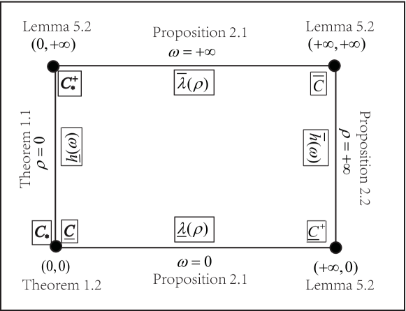
Figure 2. The illustrations of the quantities defined in (1.5) and (5.1), which are some double limit values of the principal eigenvalue $\lambda(\omega,\rho)$ when $\omega$ tends to $0$ or $+\infty$ and/or $\rho$ tends to $0$ or $+\infty$.

In addition to the notations in (1.5) and (5.1), some limit values provided in Theorem 1.1, Propositions 2.1 and 2.2 are summarized in Fig. 2, where

$$\begin{split}\underline{h}(\omega)=\lim_{\rho\to 0}\lambda(\omega,\rho),\quad\overline{h}(\omega)=\lim_{\rho\to+\infty}\lambda(\omega,\rho),\quad\forall\omega>0,\\ \underline{\lambda}(\rho)=\lim_{\omega\to 0}\lambda(\omega,\rho),\quad\overline{\lambda}(\rho)=\lim_{\omega\to+\infty}\lambda(\omega,\rho),\quad\forall\rho>0.\end{split}$$

Based on the above notations, we have the following result.

Lemma 5.3.

For each $\rho>0$, let $\overline{\lambda}(\rho)$ and $\underline{\lambda}(\rho)$ be defined in Proposition 2.1.

• If $\underline{C}<\underline{C}^{+}$, then for $\ell\in(\underline{C},\underline{C}^{+})$, there exists a unique $\rho_{\ell}>0$ such that $\underline{\lambda}(\rho_{\ell})=\ell$. Moreover, $\rho_{\ell}$ is increasing in $\ell$, $\rho_{\ell}\to 0$ as $\ell\to\underline{C}$, and $\rho_{\ell}\to+\infty$ as $\ell\to\underline{C}^{+}$.

• If $C_{*}^{+}<\overline{C}$, then for $\ell\in(C_{*}^{+},\overline{C})$, there exists a unique $\underline{\rho}_{\ell}\in(0,\rho_{\ell}]$ such that $\overline{\lambda}(\underline{\rho}_{\ell})=\ell$. Moreover, $\underline{\rho}_{\ell}$ is increasing in $\ell$, $\underline{\rho}_{\ell}\to 0$ as $\ell\to C_{*}^{+}$, and $\underline{\rho}_{\ell}\to+\infty$ as $\ell\to\overline{C}$.

Moreover, $\rho_{\ell}=\underline{\rho}_{\ell}$ if and only if (4.13) holds.

Proof.

We shall prove part (i), and part (ii) can follow by the rather similar arguments. A direct application of [9, Theorem 1] or [23, Theorem 1.4] to problem (2.2) yields $\lambda_{0}(t,\rho)\to-\max_{x\in\overline{\Omega}}\mu({\bf A}(x,t))$ as $\rho\to 0$, where $\lambda_{0}(t,\rho)$ denotes the principal eigenvalue of (2.2). Then applying Corollary 2.3 to problem (2.2), we have $\lambda_{0}(t,\rho)\to-\mu(\overline{\bf A}(t))$ as $\rho\to+\infty$. Hence, recall from the definitions in (1.5) and (5.1) that

(5.13) $$\lim_{\rho\to 0}\underline{\lambda}(\rho)=\underline{C}\quad\text{and}\quad\lim_{\rho\to+\infty}\underline{\lambda}(\rho)=\underline{C}^{+}.$$

By continuity, for each $\ell\in(\underline{C},\underline{C}^{+})$, there exists some $\rho_{\ell}>0$ such that $\underline{\lambda}(\rho_{\ell})=\ell$.

We next prove the uniqueness of such $\rho_{\ell}$. Suppose that $\underline{\lambda}(\rho_{*})=\ell$ for some $\rho_{*}\neq\rho_{\ell}$. Without loss of generality, assume $\rho_{*}<\rho_{\ell}$. Due to the symmetry of matrix ${\bf A}(x,t)$, it follows from the variational structure of (2.2) that $\lambda_{0}(t,\rho)$ is increasing in $\rho$ if ${\bf A}$ is a non-constant matrix in $x$, and otherwise $\lambda_{0}(t,\rho)$ is constant in $\rho$. Hence, $\lambda_{0}(t,\rho_{*})\leq\lambda_{0}(t,\rho_{\ell})$ for all $t\in\mathbb{R}$. By our assumption $\underline{\lambda}(\rho_{*})=\underline{\lambda}(\rho_{\ell})=\ell$, it follows that $\lambda_{0}(t,\rho_{*})=\lambda_{0}(t,\rho_{\ell})$ for all $t\in\mathbb{R}$. This implies $\lambda_{0}(t,\rho)=\lambda_{0}(t)$ independent of $\rho$, and thus $\underline{\lambda}(\rho)\equiv\ell$ for all $\rho>0$. By (5.13), one has $\underline{C}=\underline{C}^{+}=\ell$, contradicting our assumption $\underline{C}<\underline{C}^{+}$. This proves the uniqueness of $\rho_{\ell}$.

Since $\underline{\lambda}(\rho)$ is non-decreasing in $\rho$, the uniqueness of $\rho_{\ell}$ implies that $\underline{\lambda}(\rho)$ is increasing in $\rho$, and thus by definition, $\rho_{\ell}$ is increasing in $\ell$. Moreover, due to (5.13), it is clear that $\rho_{\ell}\to 0$ as $\ell\to\underline{C}$ and $\rho_{\ell}\to+\infty$ as $\ell\to\underline{C}^{+}$.

Finally, the fact that $\rho_{\ell}=\underline{\rho}_{\ell}$ if and only if (4.13) holds is a direct consequence of Theorem 4.3. Lemma 5.3 is thus proved. ∎

For each value $\ell\in(\underline{C},\overline{C})$, define the level set

$$\Sigma_{\ell}:=\{(\omega,\rho):\,\omega,\rho>0,\quad\lambda(\omega,\rho)=\ell\}.$$

Our aim is to characterize the topological structures of all level sets.

Theorem 5.4.

For any $\ell\in(\underline{C},\overline{C})$, let constants $0<\underline{\rho}_{\ell}\leq\rho_{\ell}$ be defined by Lemma 5.3 such that $\underline{\lambda}(\rho_{\ell})=\overline{\lambda}(\underline{\rho}_{\ell})=\ell$. If $\underline{\rho}_{\ell}=\rho_{\ell}$, then $\Sigma_{\ell}=\{(\omega,\rho):\,\rho=\rho_{\ell},\,\,\,\omega>0\}$; Otherwise there exist uniquely a continuous function $\omega_{\ell}:{\rm dom}(\omega_{\ell})\mapsto(0,+\infty)$ such that

$$\Sigma_{\ell}=\{(\omega,\rho):\,\omega=\omega_{\ell}(\rho),\,\,\,\rho\in{\rm dom}(\omega_{\ell})\}.$$

The domain ${\rm dom}(\omega_{\ell})$ and asymptotic behaviors of function $\omega_{\ell}$ can be characterized as follows.

• If $\ell\in(\underline{C},\min\{C_{*}^{+},\underline{C}^{+}\})$, then ${\rm dom}(\omega_{\ell})=(0,\rho_{\ell})$ and $\omega_{\ell}(\rho)\to 0$ as $\rho\nearrow\rho_{\ell}$. The asymptotic behaviors of $\omega_{\ell}(\rho)$ at $\rho=0$ are as follows.

  • If $\ell\in(\underline{C},C_{*}]$, then $\omega_{\ell}(\rho)\to 0$ as $\rho\searrow 0$. Furthermore, if $\ell\in(\underline{C},C_{*})$, there exist $0<{\underline{c}}<{\overline{c}}$ independent of $\rho$ such that ${\underline{c}}\sqrt{\rho}\leq\omega_{\ell}(\rho)\leq{\overline{c}}\sqrt{\rho}$ for small $\rho>0$.

  • If $\ell\in(C_{*},\min\{C_{*}^{+},\underline{C}^{+}\})$, then $\omega_{\ell}(\rho)\to\underline{h}^{-1}(\ell)$ as $\rho\searrow 0$.

• If $C_{*}^{+}<\underline{C}^{+}$ and $\ell\in(C_{*}^{+},\underline{C}^{+})$, then ${\rm dom}(\omega_{\ell})=(\underline{\rho}_{\ell},\rho_{\ell})$, and function $\omega_{\ell}$ satisfies $\omega_{\ell}(\rho)\to 0$ as $\rho\nearrow\rho_{\ell}$ and $\omega_{\ell}(\rho)\to+\infty$ as $\rho\searrow\underline{\rho}_{\ell}$.

• If $\underline{C}^{+}<C_{*}^{+}$ and $\ell\in[\underline{C}^{+},C_{*}^{+})$, then ${\rm dom}(\omega_{\ell})=(0,+\infty)$, and function $\omega_{\ell}$ satisfies $\omega_{\ell}(\rho)\to\underline{h}^{-1}(\ell)$ as $\rho\searrow 0$ and $\omega_{\ell}(\rho)\to\overline{h}^{-1}(\ell)$ as $\rho\nearrow+\infty$.

• If $\ell\in(\max\{C_{*}^{+},\underline{C}^{+}\},\overline{C})$, then ${\rm dom}(\omega_{\ell})=(\underline{\rho}_{\ell},+\infty)$, and function $\omega_{\ell}$ satisfies $\omega_{\ell}(\rho)\to+\infty$ as $\rho\searrow\underline{\rho}_{\ell}$ and $\omega_{\ell}(\rho)\to\overline{h}^{-1}(\ell)$ as $\rho\nearrow+\infty$.

Theorem 5.4 yields five types of topological structures for level sets $\Sigma_{\ell}$, which are illustrated by various shaded areas in Fig. 3. The pictures presented in Fig. 3 are focused on the scenarios where all quantities in (1.5) and (5.1) are distinct.

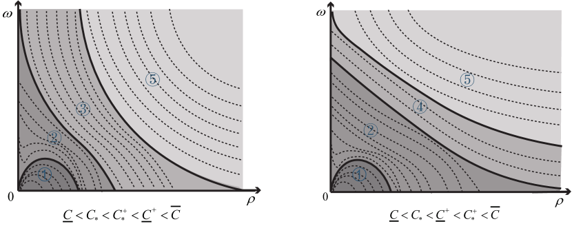
Figure 3. A sketch of the level sets of principal eigenvalue $\lambda(\omega,\rho)$ in $\rho$-$\omega$ plane as shown in Theorem 5.4, which are illustrated by the bounded or unbounded curves presenting the graphs of function $\omega=\omega_{\ell}(\rho)$ for the cases $\underline{C}<C_{*}<C_{*}^{+}<\underline{C}^{+}<\overline{C}$ and $\underline{C}<C_{*}<\underline{C}^{+}<C_{*}^{+}<\overline{C}$.

• For $\ell\in(\underline{C},C_{*})$, part (1)-(i) of Theorem 5.4 asserts all level sets $\Sigma_{\ell}$ are characterized by bounded curves connecting $(0,0)$ and $(\rho_{\ell},0)$ in $\rho$-$\omega$ plane as illustrated by curves in areas ① of Fig. 3. The estimate in part (1)-(i) indicates the curve $\omega=\omega_{\ell}(\rho)$ has asymptotic behavior of the form $\omega\sim\sqrt{\rho}$ at the origin.

• For $\ell\in(C_{*},\min\{C_{*}^{+},\underline{C}^{+}\})$, part (1)-(ii) in Theorem 5.4 suggests level sets $\Sigma_{\ell}$ are characterized by bounded curves connecting points $(\rho_{\ell},0)$ and $(0,\underline{h}^{-1}(\ell))$, which are illustrated by curves in areas ② of Fig. 3.

• For $C_{*}^{+}<\underline{C}^{+}$ and $\ell\in(C_{*}^{+},\underline{C}^{+})$, by part (2) of Theorem 5.4, the level sets $\Sigma_{\ell}$ will connect $(\rho_{\ell},0)$ and approach asymptotically to the vertical line $\rho=\underline{\rho}_{\ell}$, which are illustrated by curves in unbounded areas ③ in the left figure of Fig. 3

• For $\underline{C}^{+}<C_{*}^{+}$ and $\ell\in(\underline{C}^{+},C_{*}^{+})$, the level sets $\Sigma_{\ell}$ are illustrated by curves in unbounded areas ④ in the right figure of Fig. 3. In particular, $\Sigma_{\ell}$ will connect $(0,\underline{h}^{-1}(\ell))$ and approach asymptotically to the horizontal line $\omega=\underline{h}^{-1}(\ell)$ as proved by part (3) of Theorem 5.4.

• For $\ell\in(\max\{C_{*}^{+},\underline{C}^{+}\},\overline{C})$, part (4) of Theorem 5.4 implies the level sets $\Sigma_{\ell}$ are given by unbounded curves approaching asymptotically to both the vertical line $\rho=\underline{\rho}_{\ell}$ and the horizontal line $\omega=\underline{h}^{-1}(\ell)$, see areas ⑤ of Fig. 3.

For any $\ell\in(\underline{C},{\overline{C}})$, the topological structure of level sets $\Sigma_{\ell}$ is a combination of these five types, which are separated by the level sets $\Sigma_{C_{*}}$, $\Sigma_{C_{*}^{+}}$ and $\Sigma_{\underline{C}}$. In particular, if $C_{*}=C_{*}^{+}$ and $\underline{C}^{+}=\overline{C}$, then the corresponding structure of level sets is analogue to that of scalar case in [26] and spatially homogeneous case in [27].

We are in a position to prove Theorem 5.4.

Proof of Theorem 5.4.

Let $\overline{\lambda}(\rho)$ be the principal eigenvalue of problem (2.1) in Proposition 2.1, which serves as the limit of $\lambda(\omega,\rho)$ as $\omega\to+\infty$. By our assumption, $\widehat{\bf A}(x)$ is a symmetric matrix for all $x\in\Omega$. Hence, by the variational structure of (2.1), $\overline{\lambda}(\rho)$ is non-decreasing in $\rho$, and either $\overline{\lambda}^{\prime}(\rho)>0$ for all $\rho>0$, or $\overline{\lambda}^{\prime}(\rho)\equiv 0$. It was shown in [9, Theorem 1] or [23, Theorem 1.4] that $\overline{\lambda}(\rho)\to C_{*}^{+}$ as $\rho\to 0$, and hence

(5.14) $$C_{*}^{+}\leq\overline{\lambda}(\rho)\leq\overline{C}\quad\text{for all }\,\rho>0,$$

and $\overline{\lambda}(\rho)$ is strictly increasing in $\rho$ if $C_{*}^{+}<\overline{C}$.

Step 1. We assume $\ell\in(\underline{C},\min\{C_{*}^{+},\underline{C}^{+}\})$ and prove part (1). In view of $\underline{C}<\underline{C}^{+}$, let $\rho_{\ell}$ be determined by Lemma 5.3. Since $\underline{\lambda}(t,\rho)$ is non-decreasing in $\rho$, the uniqueness of $\rho_{\ell}$ implies

(5.15) $$\underline{\lambda}(\rho)<\underline{\lambda}(\rho_{\ell})=\ell\quad\text{for any }\,\rho\in(0,\rho_{\ell}).$$

This together with (5.14) implies that $\underline{\lambda}(\rho)<\ell\leq C_{*}^{+}\leq\overline{\lambda}(\rho)$ for all $\rho\in(0,\rho_{\ell})$. Applying the monotonicity established in Theorem 1.4, we find $\lambda(\omega,\rho)$ is strictly increasing in $\omega$ for any $\rho\in(0\rho_{\ell})$, and hence by Proposition 2.1, there is a unique continuous non-negative function $\omega_{\ell}(\rho):(0,\rho_{\ell})\mapsto[0,\infty)$ such that

(5.16) $$\lambda(\omega_{\ell}(\rho),\rho)\equiv\ell,\quad\forall\rho\in(0,\rho_{\ell}).$$

where the continuity follows from the implicit function theorem. By (5.15), it is easily seen that $\omega_{\ell}(\rho_{\ell})=0$ and $\omega_{\ell}(\rho_{\ell})>0$ for $\rho\in(0,\rho_{\ell})$. We shall prove part (1) by considering the following two cases:

Case 1: We assume $\ell\in(\underline{C},C_{*}]$ to establish part (1)-(i). We first claim $\omega_{\ell}(\rho)\to 0$ as $\rho\to 0$. If not, then there exists some sequence $\{\rho_{n}\}_{n\geq 1}$ such that $\rho_{n}\to 0$ and $\omega_{\ell}(\rho_{n})\to\omega_{*}$ as $n\to+\infty$ for some $\omega_{*}\in(0,+\infty]$. Then we shall reach a contradiction by the following two cases: (i) If $\omega_{*}=+\infty$, then a direct application of Lemma 5.2 yields $\lambda(\omega_{\ell}(\rho_{n}),\rho_{n})\to C_{*}^{+}$ as $n\to+\infty$. Note from (5.16) that $\lambda(\omega_{\ell}(\rho_{n}),\rho_{n})\equiv\ell$ for all $n$, so that $\ell=C_{*}^{+}$, which is a contradiction since $\ell<\min\{C_{*}^{+},\underline{C}^{+})$ by our assumption. (ii) If $\omega_{*}<+\infty$, it follows by Theorem 1.1 that $\lambda(\omega_{\ell}(\rho_{n}),\rho_{n})\to\underline{h}(\omega_{*})$ as $n\to+\infty$. Since $\lambda(\omega_{\ell}(\rho_{n}),\rho_{n})\equiv\ell$ for all $n$, one has $\ell=\underline{h}(\omega_{*})\leq C_{*}$. Due to the symmetry of ${\bf A}$, we can apply the monotonicity result in [28, Theorem 1.1] to (1.4) and obtain that either $\underline{h}(\omega)$ is strictly increasing in $\omega$, or $\underline{h}(\omega)$ is constant in $\omega$. Due to $\underline{h}(\omega)\to C_{*}$ as $\omega\to 0$ (by applying [28, Theorem 2.1]), it holds $\underline{h}(\omega_{*})=C_{*}$, and furthermore $\underline{h}(\omega)\equiv C_{*}$ for all $\omega>0$. By $\ell=\underline{h}(\omega_{*})$ one has $\ell=C_{*}<C_{*}+$ by our assumption. In particular, according to the fact that $\underline{h}(\omega)\to C_{*}^{+}$ as $\omega\to+\infty$, we derive $C_{*}=C_{*}^{+}$, which is a contradiction. Therefore, $\omega_{\ell}(\rho)\to 0$ as $\rho\to 0$.

It remains to prove that for the case $\ell\in(\underline{C},C_{*})$, it holds $c_{1}{\sqrt{\rho}}\leq{\omega_{\ell}(\rho)}\leq c_{2}\sqrt{\rho}$ for some constants $0<c_{1}<c_{2}$ independent of $\rho$. We first claim ${\omega_{\ell}(\rho)}\geq c_{1}{\sqrt{\rho}}$ holds for some constant $c_{1}>0$. If not, then there exists some sequence $\{\underline{\rho}_{n}\}_{n=1}^{\infty}$ such that $\omega_{\ell}(\underline{\rho}_{n})/\sqrt{\underline{\rho}_{n}}\to 0$ and $\underline{\rho}_{n}\to 0$ as $n\to+\infty$. Then a direct application of Theorem 1.2 yields $\lambda(\omega_{\ell}(\underline{\rho}_{n}),\underline{\rho}_{n})\to\underline{C}$ as $n\to+\infty$, so that $\ell=\underline{C}$, which is a contradiction. We next show $\omega_{\ell}(\rho)\leq c_{2}\sqrt{\rho}$ for some $c_{2}>0$ independent of $\rho$. Suppose on the contrary that there exists some sequence $\{\rho_{n}\}_{n=1}^{\infty}$ such that $\overline{\rho}_{n}\to 0$ and $\omega_{\ell}(\overline{\rho}_{n})/\sqrt{\overline{\rho}_{n}}\to+\infty$ as $n\to+\infty$. Then Theorem 1.2 implies $\lambda(\omega_{\ell}(\overline{\rho}_{n}),\overline{\rho}_{n})\to C_{*}$ as $n\to+\infty$, which contradicts $\lambda(\omega_{\ell}(\overline{\rho}_{n}),\overline{\rho}_{n})\equiv\ell<C_{*}$. Therefore, $0<c_{1}\leq\omega_{\ell}(\rho)/\sqrt{\rho}\leq c_{2}$. Part (1)-(i) is thus proved.

Case 2: We assume $\ell\in(C_{*},\min\{C_{*}^{+},\underline{C}^{+}\})$ to establish part (1)-(ii). Due to $C_{*}<C_{*}^{+}$, we apply [28, Theorem 1.1] to problem (1.4) and derive that $\underline{h}(\omega)$ is strictly increasing in $\omega$, with $\underline{h}(\omega)$ being defined as the limit of $\lambda(\omega,\rho)$ as $\rho\to 0$, see Theorem 1.1. Hence, there is the unique $\omega=\underline{h}^{-1}(\ell)$ such that $\underline{h}(\omega)=\ell$. Fix any sequence $\{\rho_{n}\}_{n=1}^{\infty}$ such that $\rho_{n}\to 0$ as $n\to+\infty$. If $\omega_{\ell}(\rho_{n})\to\omega_{*}$ for some $\omega_{*}\in[0,+\infty]$, then due to $\ell\in(C_{*},C_{*}^{+})$, by Theorem 1.2 and Lemma 5.2 we have $\omega_{*}\in(0,+\infty)$. Hence, Theorem 1.1 implies $\lambda(\omega_{\ell}(\rho_{n}),\rho_{n})\to\underline{h}(\omega_{*})$ as $n\to+\infty$, which together with (5.16) implies $\ell=\underline{h}(\omega_{*})$, and thus $\omega_{*}=\underline{h}^{-1}(\ell)$. This proves part (1)-(ii).

Step 2. We assume $\ell\in(C_{*}^{+},\underline{C}^{+})$ and $C_{*}^{+}<\underline{C}^{+}$ to prove part (2). In view of $\underline{C}\leq C_{*}<\underline{C}^{+}$, let $\rho_{\ell}>0$ be given by Lemma 5.3. Note that $\underline{\lambda}(\rho_{\ell})=\ell$ as given in Lemma 5.3. Let ${\bm{\phi}}>0$ be the principal eigenfunction of (2.1) with $\rho=\rho_{\ell}$. If ${\bf A}{\bm{\phi}}=\widehat{\bf A}(x){\bm{\phi}}+g(t){\bm{\phi}}$ for some $1$-periodic function $g$, Theorem 4.3(ii) yields $\lambda(\omega,\rho_{\ell})\equiv\ell$ for all $\omega>0$; Otherwise, $\lambda(\omega,\rho_{\ell})$ is strictly increasing in $\omega>0$, so that $\overline{\lambda}(\rho_{\ell})>\underline{\lambda}(\rho_{\ell})=\ell$, which implies $\underline{\rho}_{\ell}<\rho_{\ell}$. For each $\rho\in(\underline{\rho}_{\ell},\rho_{\ell})$, by (5.15) and the monotonicity of $\overline{\lambda}(\rho)$, it holds that $\underline{\lambda}(\rho)<\overline{\lambda}(\underline{\rho}_{\ell})<\overline{\lambda}(\rho)$. Hence, by the monotonicity of $\omega\mapsto\lambda(\omega,\rho)$ in Theorem 1.4, there is a unique continuous non-negative function $\omega_{\ell}(\rho):(\underline{\rho}_{\ell},\rho_{\ell}]\to[0,\infty)$ such that

(5.17) $$\lambda(\omega_{\ell}(\rho),\rho)\equiv\ell,\quad\forall\rho\in(\underline{\rho}_{\ell},\rho_{\ell}).$$

Clearly, $\omega_{\ell}(\rho_{\ell})=0$ and $\omega_{\ell}(d)>0$ for $\rho\in(\underline{\rho}_{\ell},\rho_{\ell})$. To part (2), it remains to show $\omega_{\ell}(\rho)\to+\infty$ as $\rho\searrow\underline{\rho}_{\ell}$. If not, then there exist some $\omega_{*}\geq 0$ and sequence $\{\rho_{n}\}_{n=1}^{\infty}$ such that $\rho_{n}\searrow\underline{\rho}_{\ell}$ and $\omega_{A}(\rho_{n})\to\omega_{*}$ as $n\to+\infty$. By (5.17), one has $\lambda(\omega_{*},\underline{\rho}_{\ell})=\ell$, and thus $\overline{\lambda}(\underline{\rho}_{\ell})=\lambda(\omega_{*},\underline{\rho}_{\ell})$. Applying Theorem 1.4 once again yields $\lambda(\omega,\underline{\rho}_{\ell})\equiv\ell$ for all $\omega>0$, which contradicts $\underline{\lambda}(\underline{\rho}_{\ell})<\ell$ as stated in (5.15). This proves part (2).

Step 3. We assume $\ell\in(\underline{C}^{+},C_{*}^{+})$ and $\underline{C}^{+}<C_{*}^{+}$ to prove part (3). We observe that

$$\underline{\lambda}(\rho)\leq\underline{C}^{+}<\ell<C_{*}^{+}\leq\overline{\lambda}(\rho),\quad\forall\rho>0.$$

Hence, Theorem 1.4 implies that $\lambda(\omega,\rho)$ is strictly increasing in $\omega$, and there is a unique continuous function $\omega_{\ell}(\rho):(0,+\infty)\to[0,\infty)$ such that $\lambda(\omega_{\ell}(\rho),\rho)\equiv\ell$ for all $\rho>0$.

Let $\underline{h}(\omega)$ be defined in Theorem 1.1, serving as the limit of $\lambda(\omega,\rho)$ as $\rho\to 0$. Note that

(5.18) $$\lim_{\omega\to 0}\underline{h}(\omega)=C_{*}\leq\underline{C}^{+}<\ell<C_{*}^{+}=\lim_{\omega\to+\infty}\underline{h}(\omega).$$

In view of $C_{*}\leq\underline{C}^{+}<C_{*}^{+}$, as in Step 1, we may apply [28, Theorem 1.1] to derive that $\underline{h}(\omega)$ is strictly increasing in $\omega$. This together with (5.18) yields $\underline{h}^{-1}(\ell)$ exists. By similar arguments as in Case 2 of Step 1, we find $\omega_{\ell}(\rho)\to\underline{h}^{-1}(\ell)$ as $\rho\to 0$.

It remains to show $\omega_{\ell}(\rho)\to\overline{h}^{-1}(\ell)$ as $\rho\to+\infty$, where $\overline{h}(\omega)$ is the limit of $\lambda(\omega,\rho)$ as $\rho\to+\infty$; see Proposition 2.2. Similar to (5.18), we find

$$\lim_{\omega\to 0}\overline{h}(\omega)=\underline{C}^{+}<\ell<C_{*}^{+}\leq\overline{C}=\lim_{\omega\to+\infty}\overline{h}(\omega).$$

Hence, by applying [28, Theorem 1.1] to problem (2.7) yields that $\overline{h}(\omega)$ is strictly increasing in $\omega$, so that $\overline{h}^{-1}(\ell)$ exists uniquely. Given any sequence $\{\rho_{n}\}_{n=1}^{\infty}$ such that $\rho_{n}\to+\infty$ as $n\to+\infty$. Assume $\omega_{\ell}(\rho_{n})\to\omega_{*}$ for some $\omega_{*}\in[0,+\infty]$, then due to $\ell\in(\underline{C},\overline{C})$, by Theorem 1.2 and Lemma 5.2 we have $\omega_{*}\in(0,+\infty)$. Hence, Proposition 2.2 implies $\lambda(\omega_{\ell}(\rho_{n}),\rho_{n})\to\overline{h}(\omega_{*})$ as $n\to+\infty$. In view of $\lambda(\omega_{\ell}(\rho),\rho)\equiv\ell$, this implies $\ell=\overline{h}(\omega_{*})$, and thus $\omega_{*}=\overline{h}^{-1}(\ell)$. This completes Step 3.

Step 4. We assume $\ell\in(\max\{C_{*}^{+},\underline{C}^{+}\},\overline{C})$ and prove part (4). Since $C_{*}^{+}<\overline{C}$, let $\underline{\rho}_{\ell}>0$ be defined by Lemma 5.3. Due to $\overline{\lambda}(\underline{\rho}_{\ell})=\ell$, the monotonicity of $\overline{\lambda}(\rho)$ implies $\overline{\lambda}(\rho)>\ell$ for all $\rho>\underline{\rho}_{\ell}$, and thus $\underline{\lambda}(\rho)\leq\underline{C}^{+}<\ell<\overline{\lambda}(\rho)$ for all $\rho>\underline{\rho}_{\ell}$. This together with Theorem 1.4 implies that $\lambda(\omega,\rho)$ is increasing in $\omega$, and thus there is a unique positive continuous function $\omega_{\ell}(\rho):(\underline{\rho}_{\ell},+\infty)\mapsto[0,\infty)$ such that $\lambda(\omega_{\ell}(\rho),\rho)\equiv\ell$ for all $\rho\in(\underline{\rho}_{\ell},+\infty)$. Then by the same arguments in Steps 2 and 3, we can show $\omega_{\ell}(\rho)\to+\infty$ as $\rho\to\underline{\rho}_{\ell}$ and $\omega_{\ell}(\rho)\to\overline{h}^{-1}(\ell)$ as $\rho\to+\infty$. Therefore, part (4) is proved.

The proof of Theorem 5.4 is now complete. ∎

For the temporally constant case, i.e. matrix A is independent of $t$, it can be observed that $\underline{C}=C_{*}=C_{*}^{+}$. The variational structure of (1.1) indicates that principal eigenvalue is monotone non-increasing in $\rho$. In contrast, Theorem 5.4 turns out to imply some non-monotone dependence of principal eigenvalue on $\rho$ when $\underline{C}<C_{*}$.

Corollary 5.5.

For each $x\in\Omega$ and $\omega>0$, let $h(x,\omega)$ be the principal eigenvalue of (1.4). Assume $\underline{C}<C_{*}$, then the followings hold.

• If $C_{*}=\overline{C}$, then for each $\omega>0$, $\lambda(\omega,\rho)$ attains its global minimum exactly at both $\rho=0$ and $\rho=+\infty$.

• If $C_{*}<\overline{C}$ and for each $\omega>0$, function $h(x,\omega)$ admits finite number of strict local minimal points, all of which are non-degenerate, i.e. the associated Hessian matrices are positive defined. Then for any $\omega>0$, $\lambda(\omega,\rho)$ attains a local minimum at $\rho=0$, and there exists some $\omega_{*}>0$ such that for each $0<\omega<\omega_{*}$, there exist two positive constants $0<\underline{\rho}<\overline{\rho}$ such that

  • $\lambda(\omega,\underline{\rho})=\lambda(\omega,\overline{\rho})=C_{*}$,

  • $\lambda(\omega,\rho)>C_{*}$ for all $\rho\in(0,\underline{\rho})\cup(\overline{\rho},+\infty)$, and

  • $\lambda(\omega,\rho)<C_{*}$ for some $\rho\in(\underline{\rho},\overline{\rho})$.

  In particular, $\lambda(\omega,\rho)$ attains its global minimum in $(\underline{\rho},\overline{\rho})$.

Corollary 5.5 implies that for temporally varying environment, the principal eigenvalue $\lambda(\omega,\rho)$ may not depend on diffusion rate $\rho$ monotonically, which is illustrated in Fig. 4. It could occur that $\lambda(\omega,\rho)$ is monotone decreasing for some ranges of $\rho$, and the global minimum of $\lambda(\omega,\rho)$ is attained at some intermediate value of $\rho$. This suggests the effect of diffusion rate on the principal eigenvalue of (1.1) can be rather complicate in contrast to temporally constant case.

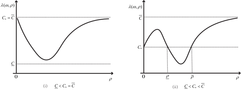
Figure 4. Graphs of $\lambda(\omega,\rho)$ as functions of $\rho$, with fixed $\omega$, for the cases given in Theorem 5.5. These figures are for illustration purpose only, as the exact shapes of the graphs could be more complex.

In what follows, we are devoted into proving Corollary 5.5. We first establish the following lower bound of $\lambda(\omega,\rho)$, which implies that for each fixed $\omega>0$, $\lambda(\omega,\rho)$ attains a local minimum at $\rho=0$.

Lemma 5.6.

For any $\omega>0$ and $x\in\overline{\Omega}$, let $h(x,\omega)$ be the principal eigenvalue of problem (1.4). Suppose the assumptions in Corollary 5.5-(ii) hold. Then for any $\omega>0$, there exist some $\eta,\rho_{0}>0$ independent of $\rho>0$ such that

(5.19) $$\lambda(\omega,\rho)>\underline{h}(\omega)+\eta\sqrt{\rho},\quad\forall\rho<\rho_{0},$$

where $\underline{h}(\omega)=\min_{x\in\overline{\Omega}}h(x,\omega)$ is the limit of $\lambda(\omega,\rho)$ as $\rho\to 0$ given by Theorem 1.1.

Proof.

Fix any $\omega>0$ throughout the proof. By our assumption, let $x_{k}\in\Omega$ ($1\leq k\leq N$) be the local minimal point such that $h(x_{k},\omega)=\underline{h}(\omega)$ and $h(x,\omega)>\underline{h}(\omega)$ for all $x\in\overline{\Omega}\setminus\{x_{1},\cdots,x_{N}\}$, as well as each point $x_{k}$ is a non-degenerate critical point. Hence, we can choose $v\in C^{2}(\overline{\Omega})$ such that for every $1\leq k\leq N$,

$$\nabla v(x_{k})=0,\quad\Delta v(x_{k})>0,\quad\nabla v\cdot\nu>0\text{ on }\partial\Omega,$$

and

(5.20) $$h(x,\omega)-\underline{h}(\omega)-\overline{d}|\nabla v|^{2}=\left\{\begin{array}[]{ll}\vskip 3.0pt plus 1.0pt minus 1.0pt+,&x\not=x_{k},\quad k=1,\cdots,N,\\ 0,&x=x_{k},\quad k=1,\cdots,N,\end{array}\right.$$

where $\overline{d}=\max\{d_{1},\cdots,d_{n}\}$. Denote by ${\bm{\phi}}=(\phi_{1},\cdots,\phi_{n})>0$ the principal eigenvector of problem (1.4) corresponding to principal eigenvalue $h(x,\omega)$. We define

$$\overline{\bm{\varphi}}(x,t):={\bm{\phi}}(x,t)\exp\left\{-\frac{v(x)}{\sqrt{\rho}}\right\},\quad\forall(x,t)\in\overline{\Omega}\times\mathbb{R}.$$

Next, we will claim there exist constants $\eta>0$ and $\rho_{0}>0$ such that for all $\rho<\rho_{0}$,

(5.21) $$\begin{cases}\begin{array}[]{ll}\vskip 3.0pt plus 1.0pt minus 1.0pt\omega\partial_{t}\overline{\bm{\varphi}}-\rho{\bf D}\Delta\overline{\bm{\varphi}}-{\bf A}\overline{\bm{\varphi}}\geq(\underline{h}(\omega)+\eta\sqrt{\rho})\overline{\bm{\varphi}}&\text{in }\,\,\Omega\times\mathbb{R},\\ \vskip 3.0pt plus 1.0pt minus 1.0pt\nabla\overline{\bm{\varphi}}\cdot\nu\geq 0&\text{on }\,\partial\Omega\times\mathbb{R},\\ \overline{\bm{\varphi}}(x,t)=\overline{\bm{\varphi}}(x,t+1)&\text{in }\,\,\Omega\times\mathbb{R}.\end{array}\end{cases}$$

Then (5.19) is a direct consequence of the comparison principle established in [2, Sect. 2].

By (1.4), direct calculations yield

$$\omega\partial_{t}\overline{\varphi}_{i}-\rho d_{i}\Delta\overline{\varphi}_{i}-\sum_{j=1}^{n}a_{ij}\overline{\varphi}_{j}-\underline{h}(\omega)\overline{\varphi}_{i}$$

$$= \omega(\partial_{t}\log\phi_{i})\overline{\varphi}_{i}-\rho d_{i}\frac{\Delta\phi_{i}}{\phi_{i}}\overline{\varphi}_{i}+2\sqrt{\rho}d_{i}(\nabla\log\phi_{i}\cdot\nabla v)\overline{\varphi}_{i}+\sqrt{\rho}d_{i}\overline{\varphi}_{i}\Delta v$$

(5.22) $$-d_{i}|\nabla v|^{2}\overline{\varphi}_{i}-\overline{\varphi}_{i}\sum_{j=1}^{n}a_{ij}\frac{\phi_{j}}{\phi_{i}}-\underline{h}(\omega)\overline{\varphi}_{i}$$

$$= \left[h(x,\omega)-\underline{h}(\omega)-d_{i}|\nabla v|^{2}\right]\overline{\varphi}_{i}$$

$$+\sqrt{\rho}d_{i}\left[\Delta v+2\nabla\log\phi_{i}\cdot\nabla v-\sqrt{\rho}\frac{\Delta\phi_{i}}{\phi_{i}}\right]\overline{\varphi}_{i},\quad\forall(x,t)\in\Omega\times\mathbb{R}.$$

By continuity, there exists some $\delta>0$ such that $\Delta v(x)\geq\Delta v(x_{k})/2$ for $x\in B_{\delta}(x_{k})$, $k=1,\cdots,N$. In view of $\nabla v(x_{k})=0$, we may further choose $\delta$ small if necessary such that $|\nabla\log\phi_{i}\cdot\nabla v|\leq\Delta v(x_{k})/4$ for all $x\in B_{\delta}(x_{k})$. Then by (5.20) and (5), there exists some $\rho_{1}>0$ small such that whenever $\rho\leq\rho_{1}$, it holds that for all $1\leq k\leq N$,

(5.23) $$\omega\partial_{t}\overline{\bm{\varphi}}-\rho{\bf D}\Delta\overline{\bm{\varphi}}-{\bf A}\overline{\bm{\varphi}}-\underline{h}(\omega)\overline{\bm{\varphi}}\geq\frac{\Delta v(x_{k})}{4}\underline{d}\sqrt{\rho}\overline{\bm{\varphi}}\quad\text{for}\,\,(x,t)\in B_{\delta}(x_{k})\times\mathbb{R}.$$

By (5.20), there exists some constant $\eta=\eta(\delta)>0$ such that

$$h(x,\omega)-\underline{h}(\omega)-\overline{d}|\nabla v|^{2}\geq\eta,\quad\forall x\not\in B_{\delta}(x_{k}),\,\,k=1,\cdots,N.$$

Hence, by (5) we may choose some constant $\rho_{2}>0$ such that for all $\rho<\rho_{2}$ and $1\leq k\leq N$,

(5.24) $$\omega\partial_{t}\overline{\bm{\varphi}}-\rho{\bf D}\Delta\overline{\bm{\varphi}}-{\bf A}\overline{\bm{\varphi}}-\underline{h}(\omega)\overline{\bm{\varphi}}\geq\frac{\eta}{2}\overline{\bm{\varphi}}\quad\text{for }\,\,x\not\in B_{\delta}(x_{k}),\ t\in\mathbb{R}.$$

Combining with (5.23) and (5.24), we have verified that the first inequality in (5.21) holds with $\rho\leq\min\{\rho_{1},\rho_{2}\}$. For $x\in\partial\Omega$ and $t\in\mathbb{R}$, observe that

$$\nabla\overline{\bm{\varphi}}\cdot\nu=\overline{\bm{\varphi}}\left[\nabla\log{\bm{\phi}}\cdot\nu-\frac{1}{\sqrt{\rho}}\nabla v\cdot\nu\right].$$

Due to $\nabla v\cdot\nu>0$, the boundary condition in (5.21) can be verified by choosing $\rho$ small. Therefore, (5.21) holds and Lemma 5.6 is proved. ∎

We conclude this section by proving Corollary 5.5.

Proof of Theorem 5.5.

We first assume $\underline{C}<C_{*}=\overline{C}$ and prove part (i). Since $C_{*}=\overline{C}$, Lemma 5.1 implies $C_{*}=C_{*}^{+}=\underline{C}^{+}=\overline{C}$, and thus by Lemma 5.2 we derive

$$\lim_{\rho\to 0}\lambda(\omega,\rho)=\lim_{\rho\to+\infty}\lambda(\omega,\rho)=\overline{C},\qquad\forall\omega>0.$$

It suffices to show $\lambda(\omega,\rho)<\overline{C}$ for all $\omega,\rho>0$. Suppose on the contrary that $\lambda(\omega_{*},\rho_{*})=\overline{C}$ for some $\omega_{*},\rho_{*}>0$. Let $\overline{\lambda}(\rho)$ be the principal eigenvalue of elliptic problem (2.1). By (5.6), $\lambda(\omega_{*},\rho_{*})\leq\overline{\lambda}(\rho_{*})\leq\overline{C}$. Due to $\lambda(\omega_{*},\rho_{*})=\overline{C}$, the monotonicity of $\omega\mapsto\lambda(\omega,\rho_{*})$ in Theorem 1.4 implies $\lambda(\omega,\rho_{*})\equiv\overline{\lambda}(\rho_{*})=\overline{C}$ for all $\omega>0$. In particular, Proposition 2.1(ii) yields

$$\overline{C}=\lim_{\omega\to 0}\lambda(\omega,\rho_{*})=\underline{\lambda}(\rho).$$

By the monotonicity of $\rho\mapsto\underline{\lambda}(\rho)$, we see that $\underline{\lambda}(\rho)\equiv\overline{C}$ for all $\rho>0$, and hence $\underline{C}=\lim_{\rho\to 0}\underline{\lambda}(\rho)=\overline{C}$. This contradicts our assumption. Part (i) thus follows.

We next show part (ii). Under the assumptions in part (ii), Lemma 5.6 implies that $\lambda(\omega,\rho)$ attains a local minimum at $\rho=0$. It remains to prove parts (a)-(c). Let $\rho_{C_{*}}$ and $\omega_{C_{*}}$ be determined by Lemma 5.3 and Theorem 5.4 with $\ell=C_{*}$. Set

(5.25) $$\omega_{*}:=\max\limits_{\rho\in[0,\rho_{C_{*}}]}\omega_{C_{*}}(\rho).$$

Then $\omega_{*}>0$ due to $\omega_{C_{*}}(0)=\omega_{C_{*}}(\rho_{C_{*}})=0$. Fix any $\omega\in(0,\omega_{*})$. We define

(5.26) $$\begin{split}\underline{\rho}:=\inf\{\rho\in(0,\rho_{C_{*}}):\,\omega_{C_{*}}(\rho)=\omega\},\quad\overline{\rho}:=\sup\{\rho\in(0,\rho_{C_{*}}):\,\omega_{C_{*}}(\rho)=\omega\}.\end{split}$$

Since $\omega<\omega_{*}$, it hold that $0<\underline{\rho}<\overline{\rho}$ and $\lambda(\omega,\underline{\rho})=\lambda(\omega,\overline{\rho})=C_{*}$, which proves part (ii)-(a).

On the other hand, it follows from (5.26) that

(5.27) $$\omega_{C_{*}}(\rho)<\omega\quad\text{and}\quad\lambda(\omega,\rho)\neq C_{*},\quad\forall\rho\in(0,\underline{\rho})\cup(\overline{\rho},\infty).$$

The monotonicity of $\omega\mapsto\lambda(\omega,\rho)$ in Theorem 1.4 implies $\lambda(\omega,\rho)>\lambda(\omega_{C_{*}(\rho)},\rho)=C_{*}$ for $\rho\in(0,\underline{\rho})\cup(\overline{\rho},\infty)$. This proves part (ii)-(b).

It suffices to show part (ii)-(c), i.e. $\lambda(\omega,\rho)<C_{*}$ for some $\rho\in(\underline{\rho},\overline{\rho})$. If not, then $\lambda(\omega,\rho)\geq C_{*}$ for all $\rho\in(\underline{\rho},\overline{\rho})$. In view of $\lambda(\omega_{C_{*}}(\rho),\rho)=C_{*}$, the monotonicity in Theorem 1.4 implies $\omega_{C_{*}}(\rho)\leq\omega$ for all $\rho\in(\underline{\rho},\overline{\rho})$. This together with (5.27) gives $\omega_{C_{*}}(\rho)\leq\omega$ for all $\rho\in(0,\rho_{C_{*}})$, which contradicts $\omega<\omega_{*}$ and (5.25). Therefore, part (ii)-(c) holds.

The proof is now complete. ∎

Acknowledgement. This work is partially supported by the NSFC grant (12201041) and Beijing Institute of Technology Research Fund Program for Young Scholars (XSQD-202214001).

References

- [1]
- [2] X. Bai, X. He, Asymptotic behavior of the principal eigenvalue for cooperative periodic-parabolic systems and applications. J. Differential Equations 269 (2020) 9868-9903.
- [3] X. Bai, X. He, W.-M. Ni, Dynamics of a periodic-parabolic Lotka-Volterra competition-diffusion system in heterogeneous environments, J. Eur. Math. Soc. 25 (2023) 4583-4637.
- [4] G. Barles, An introduction to the theory of viscosity solutions for first-order Hamilton-Jacobi equations and applications, in: Hamilton-Jacobi Equations: Approximations, Numerical Analysis and Applications, in: Lecture Notes in Math., vol. 2074, Springer, 2013, pp. 49-109.
- [5] M. Benaim, C. Lobry, T. Sari, E. Strickler, When can a population spreading across sink habitats persist? J. Math. Biol. 88 (2024) 19.
- [6] H. Berestycki, G. Nadin, Asymptotic spreading for general heterogeneous Fisher-KPP type equations, Mem. Amer. Math. Soc. 280 (1381) 2022.
- [7] R.S. Cantrell, C. Cosner, Spatial Ecology via Reaction-Diffusion Equations, Wiley Series in Mathematical and Computational Biology, John Wiley and Sons, Chichester, 2003.
- [8] M.G. Crandall, L.C. Evans, P.-L. Lions, Some properties of viscosity solutions of Hamilton-Jacobi equations, Trans. Amer. Math. Soc. 282 (1984) 487–502.
- [9] E.N. Dancer, On the principal eigenvalue of linear cooperating elliptic system with small diffusion, J. Evolut. Eqns. 9 (2009) 419-428.
- [10] J. Dockery, V. Hutson, K. Mischaikow, M. Pernarowski, The evolution of slow dispersal rates: a reaction diffusion model, J. Math. Biol. 37 (1998) 61-83.
- [11] L.C. Evans, D. Gomes, Effective Hamiltonians and averaging for Hamiltonian dynamics I, Arch. Ration. Mech. Anal. 157 (2001) 1-33.
- [12] L.C. Evans, D. Gomes, Effective Hamiltonians and averaging for Hamiltonian dynamics. II. Arch. Ration. Mech. Anal. 161 (2002) 271-305.
- [13] L.C. Evans, P.E. Souganidis, A PDE approach to geometric optics for certain semilinear parabolic equations, Indiana Univ. Math. J. 38 (1989) 141-172.
- [14] Y.-X. Feng, W.-T. Li, S. Ruan, M.-Z. Xin, Principal spectral theory of time-periodic nonlocal dispersal cooperative systems and applications, SIAM J. Math. Anal. 56 (2024) 4040-4083.
- [15] L. Girardin, I. Mazari-Fouquer, Generalized principal eigenvalues of space-time periodic, weakly coupled, cooperative, parabolic systems, arXiv:2109.09578v2.
- [16] P. Hess, Periodic-Parabolic Boundary Value Problems and Positivity, Pitman Res., Notes in Mathematics, vol. 247, Longman Sci. Tech., Harlow, 1991.
- [17] V. Hutson, K. Michaikow, P. Poláčik, The evolution of dispersal rates in a heterogeneous time-periodic environment, J. Math. Biol., 43 (2001) 501-533.
- [18] V. Hutson, W. Shen, G.T. Vickers, Estimates for the principal spectrum point for certain time-dependent parabolic operators, Proc. Amer. Math. Soc. 129 (2000) 1669-1679.
- [19] H. Ishii, Weak KAM aspects of convex Hamilton-Jacobi equations with Neumann type boundary conditions, J. Math. Pures Appl. 95 (2011) 99-135.
- [20] V.A. Jansenand, J. Yoshimura, Populations can persist in an environment consisting of sink habitats only, Proc. Natl. Acad. Sci. USA. 95 (1988) 3696-3698.
- [21] M.G. Krein, M.A. Rutman, Linear Operators Leaving Invariant a Cone in a Banach Space, American Mathematical Society, New York, 1950.
- [22] G. Katriel, Dispersal-induced growth in a time-periodic environment, J. Math. Biol. 85 (2022) 24.
- [23] K.-Y. Lam, Y. Lou, Asymptotic behavior of the principal eigenvalue for cooperative elliptic systems and applications, J. Dyn. Diff. Equat. 28 (2016) 29-48.
- [24] K.-Y. Lam, Y. Lou, Introduction to Reaction-Diffusion Equations: Theory and Applications to Spatial Ecology and Evolutionary Biology, Lecture Notes on Mathematical Modelling in the Life Sciences, Springer, Cham, 2022.
- [25] K.-Y. Lam, Y. Lou, B. Perthame, A Hamilton-Jacobi approach to evolution of dispersal, Comm. Partial Differential Equations 48 (2022) 86-118.
- [26] S. Liu, Y. Lou, Classifying the level set of principal eigenvalue for time-periodic parabolic operators and applications, J. Funct. Anal. 282 (2022) 109338.
- [27] S. Liu, Y. Lou, On the principal eigenvalues for a class of time-periodic and spatially discrete problems (in Chinese), Sci. Sin. Math. 54 (2024) 1-32.
- [28] S. Liu, Y. Lou, P. Song, A new monotonicity for principal eigenvalues with applications to time-periodic patch models, SIAM J. Appl. Math. 82 (2022) 576-601.
- [29] S. Liu, Y. Lou, R. Peng, M. Zhou, Monotonicity of the principal eigenvalue for a linear time-periodic parabolic operator, Proc. Amer. Math. Soc. 47 (2019) 5291-5302.
- [30] P.-L. Lions, Neumann type boundary conditions for Hamilton-Jacobi equations. Duke Math. J., 52 (1985) 793–820.
- [31] P.-L. Lions, G. Papanicolaou, S.R.S. Varadhan, Homogenization of Hamilton-Jacobi equations, unpublished, 1988.
- [32] D.P. Matthews, A. Gonzalez, The inflationary effects of environmental fluctuations ensure the persistence of sink metapopulations, Ecology 88 (2007) 2848-2856.
- [33] G. Nadin, The principal eigenvalue of a space-time periodic parabolic operator, Ann. Mat. Pura Appl. 188 (2009) 269-295.
- [34] R. Peng, X.-Q. Zhao, Effects of diffusion and advection on the principal eigenvalue of a periodic-parabolic problem with applications, Calc. Var. Partial Differential Equations 54 (2015) 1611-1642.
- [35] M. Roy, R.D. Holt, M. Barfield, Temporal autocorrelation can enhance the persistence and abundance of metapopulations comprised of coupled sinks, Am. Nat. 166 (2005) 246-261.
- [36] G. Sweers, Strong positivity in for elliptic systems, Math. Z. 209 (1992) 251-271.
- [37] H.V. Tran, Hamilton-Jacobi equations: theory and applications. Graduate Studies in Mathematics, 213. American Mathematical Society, Providence, RI, 2021.
- [38] L. Zhang, X.-Q. Zhao, Asymptotic behavior of the basic reproduction ratio for periodic reaction-diffusion systems, SIAM J. Math. Anal. 53 (2021) 6873-6909.
- [39] L. Zhang, X.-Q. Zhao, Asymptotic behavior of the principal eigenvalue and the basic reproduction ratio for periodic patch models. Sci. China Math. 65 (2022) 1363-1382.