A lattice QCD calculation of the Compton amplitude subtraction function

Abstract

The Compton amplitude subtraction function is an essential component in work concerning both the proton radius puzzle and the proton-neutron mass difference. However, owing to the difficulty in determining the subtraction function, it remains a key source of uncertainty in these two contexts. Here, we use the Feynman-Hellmann method to determine this subtraction function directly from lattice QCD. Furthermore, we demonstrate how to control dominant discretisation artefacts for this calculation, eliminating a major source of systematic error. This calculation is performed for a range of hard momentum scales, and three different sets of gauge configurations for pion masses about $400\;\text{MeV}$. Our results show good agreement with continuum OPE expectations. As such, this work paves the way for model-independent and precise determinations of the subtraction function over a wide range of kinematics.

I Introduction

The Compton amplitude subtraction function, $S_{1}(Q^{2})$, is a critical component in the theoretical determination of the proton–neutron mass difference, and a necessary quantity for the calculation of the proton charge radius. However, the subtraction function is not directly measurable from experiment, and as such contributes significant theoretical and statistical uncertainties to these quantities. In this context, a first-principles determination of the subtraction function could play a vital role in clarifying our understanding of hadron structure.

The leading electromagnetic contribution to the proton–neutron mass difference is given by the Cottingham sum rule Cottingham (1963)

$$\delta m^{\gamma}_{N}=-\frac{i}{2m_{p}}\frac{\alpha}{(2\pi)^{3}}\int d^{4}q\,\frac{g_{\mu\nu}T_{N}^{\mu\nu}(p,q)}{Q^{2}-i\epsilon},$$ (1)

where $T^{N}_{\mu\nu}$ is the spin-averaged forward Compton scattering amplitude for a nucleon $N(p)$

$$T^{N}_{\mu\nu}(p,q)=i\int d^{4}z\ e^{iq\cdot z}\langle N(p)|\mathcal{T}\{V_{\mu}(z)V_{\nu}(0)\}|N(p)\rangle,$$ (2)

with $V_{\mu}$ denoting the electromagnetic vector current and $q$ denoting the virtual photon 4-momentum with $Q^{2}=-q^{2}$. The subtraction function $S_{1}(Q^{2})$, defined below, encapsulates critical information about $T^{N}_{\mu\nu}$ at the $p\cdot q=0$ point.

An early evaluation of the Cottingham sum rule by Gasser and Leutwyler Gasser and Leutwyler (1975) found the electromagnetic contribution to the mass difference to be $\delta m_{N}^{\gamma}=0.76(30)\;\text{MeV}$. By contrast, a more recent evaluation Walker-Loud et al. (2012) proposed a significantly greater value, largely due to a different consideration of the Compton subtraction function. As a consequence of these developments, renewed interest was taken in the proton–neutron mass difference Thomas et al. (2015); Erben et al. (2014); Tomalak (2020); Horsley et al. (2016); Borsanyi et al. (2015). In light of further clarification Gasser et al. (2015), focusing particularly on the treatment of the subtraction function, the exact value of $\delta m_{N}^{\gamma}$ remains somewhat unclear. Thus a first-principles evaluation of $S_{1}(Q^{2})$ would be rather beneficial.

Similarly, the Compton amplitude is an input for measurements of the proton charge radius from the muonic-hydrogen Lamb shift, for which recent determinations have a 7$\sigma$ tension with results obtained via electron–proton scattering Bernauer et al. (2010); Pohl et al. (2010)—the so-called ‘proton radius puzzle’ Pohl et al. (2013); Antognini et al. (2022). This has led to renewed interest in possible systematic corrections to the muonic-hydrogen measurements, including the hadronic corrections from the two-photon exchange (TPE) Tomalak and Vanderhaeghen (2016a); Afanasev et al. (2017); Pachucki (1999), which are dependent on the forward Compton amplitude and, consequently, the subtraction function. Unfortunately, the Compton amplitude contributes the dominant uncertainty to the hadronic background, in large part due to $S_{1}(Q^{2})$ Carlson and Vanderhaeghen (2011); Hill and Paz (2011); Miller (2013). Therefore a more precise determination of the subtraction function could also help clarify the proton radius puzzle.

In both the context of the proton-neutron mass difference, and the muonic-hydrogen Lamb shift, knowledge of the Compton amplitude over the entire range of virtual photon momenta is essential. The subtraction function can be evaluated in a model independent way in the low-energy region ($Q^{2}\ll m_{p}^{2}$) from effective field theory Hill and Paz (2011), and in the high-energy region ($Q^{2}\gg\Lambda_{\text{QCD}}^{2}$) using the operator product expansion (OPE) Collins (1979); Hill and Paz (2017); Gasser et al. (2020a). In the intermediate $Q^{2}$ region various different methods have been applied including physically-motivated functional interpolations between the low and high $Q^{2}$ Walker-Loud et al. (2012); Erben et al. (2014); Hill and Paz (2017), and Regge model evaluations Gasser and Leutwyler (1975); Gasser et al. (2020a); Caprini (2021). The different methods of evaluating the unknown behaviour of the subtraction function lead to significant differences in both the proton-neutron mass difference and the two-photon exchange hadronic background.

In this context, a first-principles lattice QCD evaluation of the Compton amplitude subtraction function is crucial. Recently a lattice calculation of the subtraction function was performed using four-point correlation functions Fu et al. (2024), following on from earlier work Feng and Jin (2019); Fu et al. (2022). This calculation was performed over the range $Q^{2}\in[0,2]\,\text{GeV}^{2}$ at the physical pion mass and at an alternative subtraction point Hagelstein and Pascalutsa (2021). The resultant subtraction function was determined from a combination of lattice results and experimental data.

In this paper, we determine the Compton amplitude subtraction function over the range $1\lesssim Q^{2}\lesssim 16\,\text{GeV}^{2}$ at the standard subtraction point using the Feynman-Hellmann technique, which has previously been used to determine the structure function moments for the forward Chambers et al. (2017); Can et al. (2020); Batelaan et al. (2023) and off-forward Hannaford-Gunn et al. (2022a, 2024) Compton amplitudes. Preliminary results of our work on the Feynman-Hellmann subtraction function were first published in Ref. Hannaford-Gunn et al. (2022b). Unlike Ref. Fu et al. (2024), we do not incorporate experimental data into our subtraction function calculation, but rather present pure lattice results.

The structure of this paper is as follows: In Section II we discuss in further detail the definition of the subtraction function and its parameterisation in the high-energy region. In Section III we discuss the Feynman-Hellmann method used to determine the Compton amplitude, highlighting aspects of this implementation most relevant to the subtraction function, and initial results. Then, in Section IV, we discuss our method for correcting leading discretisation artefacts in our calculation. This is done using a lattice operator product expansion (LOPE). Finally, in Section V we remove the leading order discretisation artefacts and, in doing so, present the Compton amplitude subtraction function, and compare it with the continuum OPE expectation.

II Background

Figure 1: The diagram for proton forward Compton scattering, $\gamma^{*}(q)p(p)\to\gamma^{*}(q)p(p)$.

Our starting point is the forward virtual Compton amplitude for a proton, as shown in Eq. (2). This amplitude describes the process of photon-proton scattering, $\gamma^{*}(q)p(p)\to\gamma^{*}(q)p(p)$—see Fig. 1. By performing the standard tensor decomposition, the Compton amplitude can be written in the form Can et al. (2020)

$$\begin{split}&T_{\mu\nu}=\left(-g_{\mu\nu}+\frac{q_{\mu}q_{\nu}}{q^{2}}\right)T_{1}(\omega,Q^{2})\\ &+\frac{1}{p\cdot q}\left(p_{\mu}-\frac{p\cdot q}{q^{2}}q_{\mu}\right)\left(p_{\nu}-\frac{p\cdot q}{q^{2}}q_{\nu}\right)T_{2}(\omega,Q^{2}),\end{split}$$ (3)

where $\omega=2p\cdot q/Q^{2}$ and $Q^{2}=-q^{2}$. The alternative decomposition put forward in Ref. Gasser et al. (2020a) could provide an opportunity for future work.

The two Compton amplitude structure functions, $T_{1,2}$, satisfy the following dispersion relations Pasquini et al. (2001); Drechsel et al. (2003):

$$\begin{split}T_{1}(\omega,Q^{2})&=T_{1}(0,Q^{2})+\frac{2\omega^{2}}{\pi}\int_{1}^{\infty}d\omega^{\prime}\frac{\text{Im}T_{1}(\omega^{\prime},Q^{2})}{\omega^{\prime}(\omega^{\prime 2}-\omega^{2}-i\epsilon)},\\ T_{2}(\omega,Q^{2})&=\frac{2\omega}{\pi}\int_{1}^{\infty}d\omega^{\prime}\frac{\text{Im}T_{2}(\omega^{\prime},Q^{2})}{\omega^{\prime 2}-\omega^{2}-i\epsilon}.\end{split}$$ (4)

Crucially, the imaginary parts of $T_{1,2}$ can be determined from deep-inelastic scattering. On the other hand, $T_{1}(0,Q^{2})$ can not be experimentally accessed from inclusive processes. This is the subtraction function:

$$S_{1}(Q^{2})\equiv T_{1}(0,Q^{2}).$$ (5)

Although the subtraction function is not experimentally accessible, it can be estimated in both the low $Q^{2}$ and high $Q^{2}$ regions.

For $Q^{2}\ll m_{p}^{2}$ the subtraction function has been computed in a variety of formalisms, including effective field theory calculations Alarcon et al. (2014); Caprini (2016, 2021); Carlson and Vanderhaeghen (2011); Erben et al. (2014); Hill and Paz (2011); Gasser and Leutwyler (1975); Miller (2013); Thomas et al. (2015); Tomalak and Vanderhaeghen (2016b); Tomalak (2020); Walker-Loud et al. (2012); Walker-Loud (2019). These calculations have sizeable errors and are not always consistent with one another Gasser et al. (2020a).

In the region $Q^{2}\gg\Lambda_{\text{QCD}}^{2}$ the subtraction function can be evaluated model-independently using the operator product expansion (OPE). Such an expansion is performed in powers of $m_{p}^{2}/Q^{2}$, with the predicted asymptotic behaviour

$$S_{1}(Q^{2})\sim\frac{m_{p}^{2}}{Q^{2}},\quad\text{for}\quad Q^{2}\gg\Lambda_{\text{QCD}}^{2}.$$ (6)

Collins Collins (1979) originally determined the leading-order $m_{p}^{2}/Q^{2}$ contribution from the OPE. Hill and Paz later corrected this calculation, again only evaluating the leading $m_{p}^{2}/Q^{2}$ term. Up to gluon contributions which are suppressed by $\alpha_{s}$, the OPE result can be written Hill and Paz (2017)

$$S^{\text{OPE}}_{1}(Q^{2})=\frac{4m_{p}^{2}}{Q^{2}}\sum_{q}\mathcal{Q}_{q}^{2}\left(\langle x\rangle_{q}-\frac{m_{q}}{m_{p}}g^{q}_{S}\right),$$ (7)

where $\langle x\rangle_{q}$ is the second parton distribution function moment (i.e. the momentum fraction), $m_{q}$ is the quark mass and $g^{q}_{S}$ is the scalar charge—all for a quark of flavour $q$ and charge $\mathcal{Q}_{q}$.

Note that the expression in Eq. (7) is only the leading-order in $m_{p}^{2}/Q^{2}$ contribution to the OPE prediction. There are higher order terms in $m_{p}^{2}/Q^{2}$ that may contribute significantly, especially for $Q^{2}$ on the threshold of the perturbative region.

At low energies, in addition to the OPE contribution, there is also an elastic contribution to the subtraction function Walker-Loud et al. (2012); Erben et al. (2014); Gasser et al. (2020b, 2015)

III Feynman-Hellmann method

The Feynman-Hellmann (FH) method is a powerful tool that presents an alternative to the direct calculation of three- and four-point functions in lattice QCD. In particular, Feynman-Hellmann has proven particularly important in the case of matrix elements with two current insertions such as the Compton amplitude Chambers et al. (2017); Can et al. (2020); Batelaan et al. (2023); Hannaford-Gunn et al. (2022a, 2024).

Here we summarise the main aspects of our application of the Feynman-Hellmann method, noting that the full details can be found in Ref. Can et al. (2020). The starting point is to perturb the action, $\mathcal{S}$, by introducing external fields that couple to the valence quarks of the nucleon. For a particular choice of external field, Eq. (8), the ground-state energy of the nucleon in the external field can be related to the Compton amplitude, and thus the subtraction function, as demonstrated in Ref. Can et al. (2020). To access the flavour-diagonal piece and the flavour-mixed piece of the Compton amplitude, we perturb the action by

$$\begin{split}\mathcal{S}(\lambda)&=\mathcal{S}+\lambda_{q}\int d^{3}z\,\left(e^{i\mathbf{q}\cdot\mathbf{z}}+e^{-i\mathbf{q}\cdot\mathbf{z}}\right)V^{q}_{\mu}(z),\\ \mathcal{S}(\lambda)&=\mathcal{S}+\sum_{q}\lambda_{q}\int d^{3}z\,\left(e^{i\mathbf{q}\cdot\mathbf{z}}+e^{-i\mathbf{q}\cdot\mathbf{z}}\right)V^{q}_{\mu}(z)\end{split}$$ (8)

respectively, noting that $\mathbf{q}$ is the 3-momentum carried by the external current, and $V^{q}_{\mu}=Z_{V}\bar{\psi}^{q}\gamma_{\mu}\psi^{q}$ is the local Euclidean vector current of the quark $q=u,d$ for some choice of Lorentz index $\mu$ and with $Z_{V}$ denoting the renormalisation constant.

We implement these action modifications on the level of quark propagators

$$S^{q}_{\lambda_{q}}(z_{n}-z_{m})=\big{[}M-\lambda_{q}\mathcal{O}\big{]}^{-1}_{n,m},$$ (9)

where $M$ is the fermion matrix, $n,m$ are lattice sites and $\lambda_{q}$ is the FH coupling.

With the quark propagator in Eq. (9), the perturbed proton correlators for different flavour combinations are written generally, up to spin/colour structure, as

$$\begin{split}\mathcal{G}(\lambda_{u},\lambda_{d})\sim\langle S^{u}_{\lambda_{u}}S^{u}_{\lambda_{u}}S^{d}_{\lambda_{d}}\rangle\end{split}$$ (10)

where, for example, the flavour combination $uu$ is given by $\mathcal{G}(\lambda_{u},0)\sim\langle S^{u}_{\lambda_{u}}S^{u}_{\lambda_{u}}S^{d}\rangle$, with $S_{d}$ denoting the unperturbed down-quark propagator. Applying the general principles of Refs. Can et al. (2020); Batelaan et al. (2023), we can write the ground state energy of the nucleon in the external field as

$$E(\lambda_{u},\lambda_{d}) =m_{p}-\frac{\lambda_{u}^{2}}{2m_{p}}S^{uu}_{1}(Q^{2})-\frac{\lambda_{d}^{2}}{2m_{p}}S^{dd}_{1}(Q^{2})$$

$$-\frac{\lambda_{u}\lambda_{d}}{2m_{p}}\big{[}S^{ud}_{1}(Q^{2})+S^{du}_{1}(Q^{2})\big{]}+...,$$ (11)

noting that the ellipsis denotes terms of higher order in $\lambda$, $S^{ud}_{1}(Q^{2})=S^{du}_{1}(Q^{2})$, and where $S^{qq^{\prime}}_{1}(Q^{2})$ is the contribution to the subtraction function from

$$T^{qq^{\prime}}_{\mu\nu}(p,q)=i\int d^{4}z\ e^{iq\cdot z}\langle N(p)|\mathcal{T}\{V^{q}_{\mu}(z)V^{q^{\prime}}_{\nu}(0)\}|N(p)\rangle.$$ (12)

This Feynman-Hellmann relation is only strictly valid when the sink momentum is $\mathbf{p}=\bm{0}$. Information on the $\mathbf{p}\neq\bm{0}$ case can be found in Ref. Can et al. (2020). By definition $q_{4}=0$ in the FH procedure and hence the probe scale is given by $Q^{2}=|\mathbf{q}|^{2}$. As explained further in the following section, in our calculations we imposed a sink momentum of $\mathbf{p}=\bm{0}$ which, with $q_{4}=0$, ensures $\omega=0$.

The proton subtraction function, up to disconnected contributions, is then constructed via

$$\begin{split}&S_{1}^{p}(Q^{2})=\sum_{q,q^{\prime}=u,d}\mathcal{Q}_{q}\mathcal{Q}_{q^{\prime}}S^{qq^{\prime}}_{1}(Q^{2})\\ &=\frac{4}{9}S_{1}^{uu}(Q^{2})+\frac{1}{9}S_{1}^{dd}(Q^{2})-\frac{2}{9}\bigg{(}S_{1}^{ud}(Q^{2})+S_{1}^{du}(Q^{2})\bigg{)}.\end{split}$$ (13)

Figure 2: Lattice diagrams for all possible types of current insertion. Only Type I and Type II are considered here.

In terms of the diagrams in Fig. 2, the different flavour combinations receive the contributions,

• $uu$: Type I – V,

• $dd$: Type I, III – V

• $ud$: Type II – IV.

This distinction is particularly relevant to our discussion of lattice artefacts. In the present work, we only consider modifications to the action on the quark propagators, but not the shift in the fermion determinant which will affect the gauge field sampling. Our calculation therefore only considers diagrams of Type I and Type II in Fig. 2. In addition, Type III and Type IV contributions can be ignored in the present calculation, as they vanish at the SU(3) symmetric point. Since heavier quark contributions only appear in the final three types of Fig. 2, Eq. (13) need only include the up and down quark contributions.

Lattice determination

To determine the flavour-diagonal and flavour-mixed Compton amplitude subtraction functions, we calculate the following ratios of nucleon correlators,

$$\mathcal{R}^{uu}_{\lambda} =\frac{\mathcal{G}(\lambda,0)\mathcal{G}(-\lambda,0)}{[\mathcal{G}(0,0)]^{2}}\xrightarrow{t\gg a}A^{uu}e^{-2\Delta E_{\lambda}^{uu}t}$$

$$\mathcal{R}^{dd}_{\lambda} =\frac{\mathcal{G}(0,\lambda)\mathcal{G}(0,-\lambda)}{[\mathcal{G}(0,0)]^{2}}\xrightarrow{t\gg a}A^{dd}e^{-2\Delta E_{\lambda}^{dd}t}$$ (14)

$$\mathcal{R}^{ud}_{\lambda} =\frac{\mathcal{G}(\lambda,\lambda)\mathcal{G}(-\lambda,-\lambda)}{\mathcal{G}(\lambda,-\lambda)\mathcal{G}(-\lambda,\lambda)}\xrightarrow{t\gg a}A^{ud}e^{-4\Delta E_{\lambda}^{ud}t}$$

as a function of Euclidean time $t$ for each value of the external coupling strength $\lambda$. Then the energy shifts are

$$\begin{split}\Delta E^{uu}_{\lambda}&=\lambda^{2}\left.\frac{\partial^{2}E(\lambda,0)}{\partial\lambda^{2}}\right|_{\lambda={0}}+\mathcal{O}\left(\lambda^{4}\right),\\ \Delta E^{dd}_{\lambda}&=\lambda^{2}\left.\frac{\partial^{2}E(0,\lambda)}{\partial\lambda^{2}}\right|_{\lambda={0}}+\mathcal{O}\left(\lambda^{4}\right),\\ \Delta E^{ud}_{\lambda}&=\lambda^{2}\left.\frac{\partial^{2}E(\lambda_{1},\lambda_{2})}{\partial\lambda_{1}\partial\lambda_{2}}\right|_{\lambda_{1}=\lambda_{2}=0}+\mathcal{O}\left(\lambda^{4}\right),\end{split}$$ (15)

which from Eq. (11) are directly proportional to the subtraction function.

Subtraction Function Results

Table 1: Lattice parameters of the gauge ensembles used in this work Bietenholz et al. (2011), including $m_{p}$ Batelaan (2023), $Z_{V}$ Bickerton (2020), $g_{S}$ Smail et al. (2023) and $\langle x\rangle$ Dragos et al. (2016).

$$\begin{array}[]{c c c c c c c c c c c c c}N_{f}&N_{L}^{3}\times N_{T}&a\,[\text{fm}]&\beta&\kappa_{\ell},\kappa_{s}&am_{p}&am_{0}&m_{\pi}\,[\text{MeV}]&Z_{V}&g^{u}_{S}&g^{d}_{S}&\langle x\rangle_{u}&\langle x\rangle_{d}\\ \hline\cr\hline\cr 2+1&32^{3}\times 64&0.074&5.50&0.120900&0.4646(43)&0.00674(7)&470&0.85&4.26(10)&2.77(7)&-&-\\ 2+1&48^{3}\times 96&0.068&5.65&0.122005&0.3860(44)&0.00545(15)&410&0.86&4.83(23)&3.15(14)&0.403(1)&0.173(5)\\ 2+1&48^{3}\times 96&0.058&5.80&0.122810&0.3552(27)&0.00574(5)&430&0.88&4.47(28)&2.90(17)&-&-\\ \end{array}$$

We perform our calculation of the proton subtraction function on three gauge ensembles generated by the QCDSF collaboration Bietenholz et al. (2011). All ensembles have $2+1$ quark flavours at the SU(3) flavour symmetric point, and have an unphysical pion mass—approximately three times the physical pion mass. In expectation of the presence of large discretisation artefacts, we utilise three ensembles with relatively fine values of the lattice spacing: $a=0.074,0.068,0.058\;\text{fm}$. See Table 1 for more details.

For each gauge ensemble, we determine the subtraction function for a set of $Q^{2}$ values given in Table 2. The overall range of kinematics is $1\lesssim Q^{2}\lesssim 16\;\text{GeV}^{2}$, which pushes below the threshold of the perturbative region, and up to the region where we expect the only significant contributions to be from the OPE, Eq. (7). To determine the subtraction function we extract the energy shifts for each $\mathbf{q}$ following the methodology given in Section III for two values of the external coupling $\lambda\in[0.0125,0.0250]$ as has been done in the same way in previous Feynman-Hellmann calculations of the Compton amplitude Can et al. (2020); Batelaan et al. (2023). A single plateau fit is performed to each ratio given in Eq. (14) with the plateau regions chosen following a covariance-matrix based $\chi^{2}$ analysis. This allows us to perform simple quadratic fits in $\lambda$ to determine the subtraction functions following Eqs. (11) and (15).

Table 2: Kinematics for the all the results in this work.

$\kappa=0.120900$ $\beta=5.50$ $\mathbf{q}$ $Q^{2}$ $[2\pi/L]$ $[\mathrm{GeV}^{2}]$ $(2,0,0)$ $1.10$ $(2,1,0)$ $1.37$ $(3,1,0)$ $2.74$ $(3,2,0)$ $3.57$ $(4,0,0)$ $4.39$ $(4,1,0)$ $4.66$ $(4,2,0)$ $5.48$ $(4,3,0)$ $6.86$ $(5,1,0)$ $7.13$ $(6,3,0)$ $12.3$ $(7,3,0)$ $15.9$   $\kappa=0.122005$ $\beta=5.65$ $\mathbf{q}$ $Q^{2}$ $[2\pi/L]$ $[\mathrm{GeV}^{2}]$ $(3,1,0)$ $1.43$ $(3,2,0)$ $1.86$ $(4,2,0)$ $2.86$ $(4,3,0)$ $4.86$ $(7,1,0)$ $7.14$ $(7,4,0)$ $9.29$   $\kappa=0.122810$ $\beta=5.80$ $\mathbf{q}$ $Q^{2}$ $[2\pi/L]$ $[\mathrm{GeV}^{2}]$ $(4,3,0)$ $4.81$ $(5,3,0)$ $6.54$ $(7,1,0)$ $9.62$

In Fig. 3, we present our results for the $uu$, $dd$ and $ud$ components of the lattice subtraction function. We can see in both the $uu$ and $dd$ results that, instead of the expected asymptotic behaviour $S_{1}(Q^{2})\sim Q^{-2}$, the results appear to trend towards a large non-zero constant: $S_{1}^{uu}(Q^{2})\approx-2.5$ and $S_{1}^{dd}(Q^{2})\approx-1.5$. In contrast, the $ud$ result trends asymptotically to zero very quickly for $Q^{2}\gtrsim 4$. These results are discussed in the following sections.

Figure 3: The lattice subtraction function as determined from Feynman-Hellmann. Results are labelled according to which quark flavour the currents couple to: $u$ for both (top), $d$ for both (middle), and one on each (bottom).

Although the lattice spacing varies by more than $20\%$ across the three sets of gauge configurations ($a=0.074,0.068,0.058\;\text{fm}$), the trend of our values becoming smaller as the lattice spacing becomes finer is rather subtle, and difficult to discern. Such a result naturally suggests the presence of discretisation artefacts which converge somewhat slowly.

IV Discretisation artefacts

As with all lattice calculations, it is necessary to take into account, and correct for, discretisation artefacts present in the results. The subtraction function, more so than other quantities, suffers from such artefacts to a large degree. This is analogous to short-distance artefacts studied in the case of the hadronic vacuum polarisation Alexandrou et al. (2023); Cè et al. (2021).

To correct these artefacts, we perform a lattice operator product expansion (LOPE) of the Compton amplitude for Wilson fermions. This calculation is essentially a tree-level OPE, where the intermediate quark propagators are taken to be Wilson fermions. This section is inspired by, and builds upon, a previous LOPE by some of us in 2006 of the lattice Compton amplitude for the conserved current Göckeler et al. (2006). In contrast to this prior result, our current LOPE is specifically for the local current $V_{\mu}=Z_{V}\bar{\psi}\gamma_{\mu}\psi$ in order to match the Feynman-Hellmann calculation. Furthermore, we improve on the 2006 result by retaining the bare quark mass.

A succinct outline of the method we use to perform this LOPE is as follows (see Appendix A for further details): first, we expand and discretise the forward Compton amplitude ($T_{\mu\nu}\rightarrow T^{L}_{\mu\nu}$), then insert the Wilson form of the fermion propagators. Next, we begin the OPE by performing a Taylor expansion in small $\sin(ap_{\mu})$ (the lattice equivalent of $ap_{\mu}$ in the continuum) and substitute this expansion into the Compton amplitude ($T_{\mu\nu}^{L}\rightarrow T_{\mu\nu}^{\text{LOPE}})$. Unlike the standard OPE, which uses a hard scale $Q^{2}\rightarrow\infty$, we use a soft scale with $\sin(ap_{\mu})$ much smaller than the momentum transfer $q$. After much simplification, we associate the $\sin(ap_{\mu})$ terms with the covariant derivative before concluding by writing the relevant terms as symmetric and traceless operators.

In our full calculation in Appendix A, we restrict ourselves to terms up to first order in the covariant derivative. Then, to isolate the contribution to the subtraction function, we select the $\mu=\nu=3$ component with the constraint $q_{3}=0$ and $p_{3}=0$, which follows from the lattice sink momentum $\mathbf{p}=\mathbf{0}$. Recalling the form of Eq. (3), this unique selection (with $\omega=0$, since $q^{4}=0$ and $\mathbf{p}=\mathbf{0}$) ensures that $T^{\text{LOPE}}_{33}$ is, in fact, the LOPE of the lattice Compton subtraction function. After removing all terms present in the continuum, we are finally left with a ‘correction term’, $\Delta S_{1}$, which quantifies—to leading order—the discretisation artefact present in our lattice calculation of the subtraction function. That is, $\Delta S_{1}=S_{1}^{\text{full}}-S_{1}^{\text{cont.}}$, where $S_{1}^{\text{full}}$ is the leading order LOPE result, and $S_{1}^{\text{cont.}}$ is the leading order continuum component of the LOPE, leaving only the discretisation contribution. This result is as follows (see Eq. (44)):

$$\Delta S_{1}=C_{W}(q,m_{0})Z_{V}^{2}\langle p|\bar{\psi}\psi|p\rangle,$$ (16)

where $C_{W}(q,m_{0})$ is the Wilson coefficient of the form

$$C_{W}(q,m_{0})=\frac{2r\sum_{\rho}\left[1-\cos(aq_{\rho})\right]}{\sum_{\rho}\sin^{2}(aq_{\rho})+a^{2}M^{2}(q,m_{0})}.$$ (17)

with $M(k,m_{0})=m_{0}+\frac{r}{a}\sum_{\tau}\big{[}1-\cos(ak_{\tau})\big{]}$ and $r$ denoting the scalar Wilson coefficient. This scalar coefficient is typically set to $r=1$ in lattice simulations, but we keep it explicit in our LOPE expressions in order to keep track of $\mathcal{O}(a)$ terms arising from the Wilson term in the fermion action. Unlike standard Wilson coefficients, we also keep the bare quark mass explicit.

The correction term in Eq. (16) is comparable to the corresponding expression in Ref. Capitani et al. (2001). Under the same kinematic conditions, the 2006 result Göckeler et al. (2006) (ignoring the seagull term) is in agreement with Eq (16) in the limit $m_{0}\rightarrow 0$, as anticipated. This expression in Eq. (16) is also purely unphysical, as Taylor expanding in $a$ yields terms of order $\mathcal{O}(a)$, which vanish in the continuum. Furthermore, the expression in Eq. (16) is specifically a Wilson discretisation artefact, $\Delta S_{1}\,\propto\,r$, and thus there is an additional necessity for the term to vanish in the continuum Feng (2024). We intend to further investigate the correction in light of clover fermions Capitani et al. (2001), and for Ginsparg-Wilson fermions, for which $\mathcal{O}(a)$ contributions have already been determined Capitani et al. (2000). The matrix element is given by $\langle p|\bar{\psi}\psi|p\rangle=2am_{p}g_{S}^{\text{bare}}$, where $g_{S}^{\text{bare}}$ is the unrenormalised scalar charge. Since $am_{p}\approx 0.4$ in our calculations, we note that these artefacts will be relatively large, even at somewhat fine lattice spacings.

Taking our lattice calculations of the subtraction function, $S_{1}^{L}(Q^{2})$, we can now remove the leading order discretisation artefact, $\Delta S_{1}$, to produced an improved result

$$S^{\text{imp}}_{1}(Q^{2})=S^{L}_{1}(Q^{2})+\Delta S_{1}.$$ (18)

Since the $\mathcal{O}(a)$ term of our LOPE arises from the quark propagator connecting the two current insertions (Type I in Fig. 2), this correction only affects the $uu$ and $dd$ flavour combinations, but not the $ud$ combination. This quantitatively explains the behaviour of the results in Fig. 3, which appears reasonable in the $ud$ case, but has completely anomalous asymptotes in the $uu$ and $dd$ plots.

Figure 4: Comparison of our 2006 LOPE Göckeler et al. (2006), our lattice OPE, $\Delta S^{(\mathrm{ff})}_{1}$, in Eq. (20), and the Feynman-Hellmann results, ${S}_{1}^{L\,(\mathrm{ff})}$. Results are for free fermions and ${\mathbf{q}}=\frac{2\pi}{L}(5,1,0)$.

Figure 5: Comparison of the LOPE corection, $\Delta S_{1}^{(\text{ff})}$, and the Feynman-Hellmann (FH) results, for a free fermion over a range of ${\mathbf{q}}$ values.

Free fermion

To investigate the effectiveness of the LOPE correction $\Delta S_{1}$, we briefly consider the simple case of the free fermion. Applying simple QED, we can derive an analytic form of the forward Compton amplitude $T_{\mu\nu}$ which, under the conditions $\mu=\nu=3$ and $p_{3}=q_{3}=0$, reduces to $T_{33}=2\omega^{2}/(1-\omega^{2})$. At the subtraction point, $\omega=0$, the amplitude for a free fermion (ff) therefore vanishes. Setting $S_{1}^{\text{imp}}=0$, Eq. (18) then reduces to:

$$S_{1}^{L\,(\mathrm{ff})}(Q^{2})=-\Delta S^{(\mathrm{ff})}_{1},$$ (19)

where $S_{1}^{L\,(\mathrm{ff})}(Q^{2})$ is the free fermion lattice calculation of the subtraction function, which can be determined from Feynman-Hellmann using a single perturbed propagator as in Eq. (9) (i.e. we do not form multiple Wick contractions as in a hadron), and using unit gauge fields, $U_{\mu}=\mathbb{I}$, in the fermion matrix. We perform this calculation with a lattice size $N_{L}^{3}\times N_{T}=32^{3}\times 64$, and for values of the hopping parameter, $\kappa$, in the range $\kappa=0.0956-0.1248$, which correspond to dimensionless bare masses in the range $am=0.0064-0.5$. The results of this calculation are shown as the hollow data points in Fig. 4. As for $\Delta S^{(\mathrm{ff})}_{1}$, up to higher order corrections in $a$, it takes the form

$$\Delta S^{(\mathrm{ff})}_{1}=C_{W}(q,m_{0})2(am_{0})g_{S}^{\text{bare}}$$ (20)

where $m_{0}$ is the free fermion mass and we have taken $g_{S}^{\text{bare}}=(1+am_{0})^{-1}$ and $r=1$.

In Fig. 4 we plot the FH results, the discretisation artefact in Eq. (20) (solid curve) and our 2006 result (broken curve). We observe that, as a function of $am_{0}$, the LOPE agrees well with the numerical Feynman-Hellmann results up to $am_{0}\approx 0.5$. Comparing this LOPE with our 2006 LOPE result (which did not include the bare mass contribution) also suggests an improvement in the correction. Similarly, in Fig. 5 we see a strong agreement between $S_{1}^{L\,(\mathrm{ff})}(Q^{2})$ and $\Delta S^{(\mathrm{ff})}_{1}$ as a function of $\mathbf{q}^{2}$. For the smallest $am_{0}$ ($\kappa=0.1248$) in particular, the agreement is excellent, and also holds to large $\mathbf{q}^{2}$. It’s also interesting to note that, despite minor fluctuations in $\Delta S^{(\mathrm{ff})}_{1}$, the discretisation artefacts for the greater $am_{0}$ results are largely $\mathbf{q}^{2}$-independent.

For the free fermion we expect a strong agreement between the LOPE and numerical Feynman-Hellmann results, as $S_{1}^{L\,(\mathrm{ff})}(Q^{2})$ vanishes in the continuum. Therefore, the agreement of these results suggest that the LOPE is a good parameterisation of our dominant discretisation artefacts, both in terms of the larger $\mathcal{O}(am_{0})$ artefacts as well as the smaller $\mathcal{O}(a\mathbf{q})$ effects.

V Proton subtraction function

We present the application of the LOPE expressions to the $uu$ and $dd$ subtraction function results obtained in Section III, and conclude by constructing the proton subtraction function.

V.1 Evaluation of the discretisation artefact

Figure 6: The two components of the leading lattice artefact to our calculation as in Eq. (16). The upper panel shows $C_{W}(q,m_{0})$ for each kinematic point reported in Table 2, while the lower panel depicts $Z_{V}^{2}\langle p|\bar{\psi}\psi|p\rangle$. The total lattice artefact is given by $\Delta S_{1}=C_{W}(q,m_{0})2(am_{p})Z_{V}^{2}g_{S}$.

In Section IV, we derived a form for the leading discretisation artefact to our subtraction function, Eq. (16), which for the proton takes the form $\Delta S_{1}=C_{W}(q,m_{0})2(am_{p})Z_{V}^{2}g^{\text{bare}}_{S}$. The Wilson coefficient is determined by inserting the dimensionless $a\mathbf{q}$ vectors and the bare quark masses into Eq. (17). For our lattices the bare quark masses are extremely small: $am_{0}=0.00674,0.00545,0.00574$, for the $\beta=5.5,5.65,5.80$ ensembles, respectively. This makes the effects of the quark mass on $C_{W}(q,m_{0})$ quite small. For the matrix element $Z_{V}^{2}\langle p|\bar{\psi}\psi|p\rangle$ we determine the nucleon mass and vector renormalisation factor for each gauge ensemble separately. The bare scalar charge, $g_{S}^{\text{bare}}$, has been determined previously from a first-order Feynman-Hellmann calculation again for each of the ensembles Smail et al. (2023). The lattice parameters are shown in Tab. 1

In the top panel of Fig. 6, we plot the Wilson coefficient, $C_{W}(q,m_{0})$, against the $Q^{2}$ values for all three gauge ensembles. We see in Fig. 6 that the Wilson coefficient varies by as much as $12\%$ among the different $\mathbf{q}$ vectors, but smaller ‘jitters’ of $\sim 5\%$ are more typical.

In the bottom panel of Fig. 6, we plot the matrix element, $Z_{V}^{2}\langle p|\bar{\psi}\psi|p\rangle$, against the lattice spacing $a$. We see that there is a slight linear dependence of the matrix element on the lattice spacing $a$. Thus we anticipate a slightly larger correction to the lattice results at a larger lattice spacing, as is suggested by Fig. 3. Moreover, the ‘jitters’ we see in the Wilson coefficient largely explain the small fluctuations with $Q^{2}$ in our lattice subtraction function.

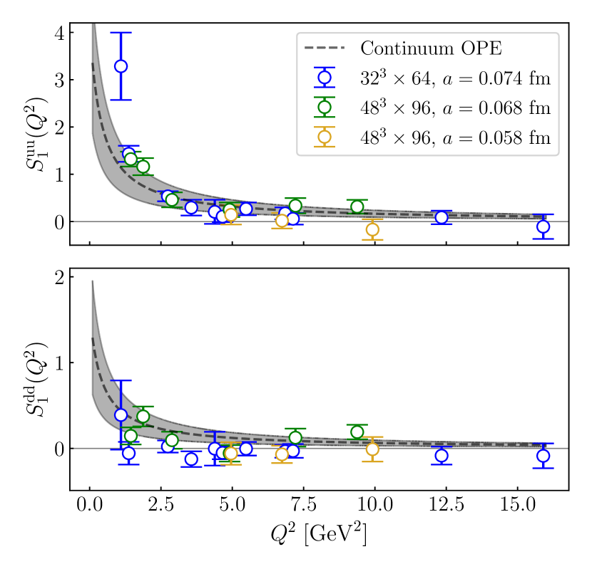
Figure 7: The subtraction function as determined from Feynman-Hellmann with lattice artefacts removed according to Eq. (18). The continuum OPE curve is also plotted, calculated directly from Eq. (7) Hill and Paz (2017) using inputs from the $a=0.074\;\text{fm}$ configurations listed in Table  1. As the scalar charge is flavour dependent, we present the results for both quark flavours ($u$ and $d$).

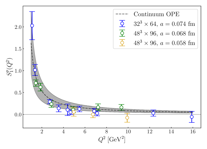
Figure 8: The proton subtraction function as determined from Feynman-Hellmann with lattice artefacts removed according to Eq. (18) and models included Hill and Paz (2017).

V.2 Improved subtraction function

Finally, we determine the improved subtraction function by removing the $\mathcal{O}(a)$ discretisation artefacts calculated in Section IV using Eq. (18). Combining the direct lattice subtraction function, Fig. 3, with the leading discretisation artefacts, Fig. 6, we present our final results for the up ($uu$) and down ($dd$) contributions in Fig. 7, and for the proton in Fig. 8. Included in both plots (dotted curve) is the continuum OPE calculated from Eq. (7).

We immediately observe an improvement in the Fig. 7 results as compared to Fig. 3, with the asymptotic $Q^{-2}$ behaviour restored for large momentum. Putting the results together to determine the subtraction function of the proton, Fig. 8, we observe a similar phenomenon. It appears as though $S_{1}(Q^{2})$ follows rather simple $Q^{-2}$ behaviour down to $Q^{2}\approx 1\,\text{GeV}^{2}$. Given the large size of the leading discretisation artefacts in Fig. 6, removing these artefacts from Fig. 3 is sufficient to shift the points upwards into the positive domain. This upwards shift brings the results into remarkable agreement with the continuum OPE in Ref. Hill and Paz (2017). Furthermore, the three sets of results at different lattice spacings are very consistent with each other.

Over the intermediate $Q^{2}$ values in Fig. 8, the proton subtraction function is rather well behaved, and a simple $Q^{-2}$ curve appears sufficient to capture the behaviour of the function.

VI Summary and Conclusions

By applying the Feynman-Hellmann method to the forward Compton amplitude, we have presented a determination of the subtraction function from first-principles. Furthermore, by performing a LOPE of the forward Compton amplitude, we successfully quantified and removed leading order Wilson discretisation artefacts, thereby placing the raw lattice results in agreement with predictions. In doing so, we demonstrated that the subtraction function indeed follows an asymptotic $Q^{-2}$ behaviour both at large $Q^{2}$ as well as intermediate momenta. Furthermore, the result indicates a smooth transition between the low and high $Q^{2}$ regimes. The results presented here established a pathway for improved lattice calculations of the subtraction function to deliver improved estimates of the proton-neutron mass difference and the proton charge radius.

Appendix A Details of Lattice Operator Product Expansion

Applying the fundamental thesis of the Operator Product Expansion (OPE), the time-ordered product of two local operators, $\mathcal{O}_{1}(z)$ and $\mathcal{O}_{2}(0)$, can be represented by a single local operator in the limit $z\rightarrow 0$. Writing this single operator in terms of a standard basis of operators, $\{\mathcal{O}_{n}\}$, the OPE can be expressed as

$$\lim_{z\rightarrow 0}\mathcal{T}\{\mathcal{O}_{1}(z)\mathcal{O}_{2}(0)\}=\sum_{n}C_{n}(z)\mathcal{O}_{n}(0),$$ (21)

where the Wilson coefficients $C_{n}(z)$ are c-number functions. Provided the external momentum of the system is small compared to the separation scale $1/z$, the perturbative, short-distance physics is entirely encoded within the Wilson coefficients, while the non-perturbative, long-distance physics is entirely contained within the operators. Of course, since QCD is an asymptotically free theory, the strong coupling constant $\alpha_{s}$ is small at the scale of $z$ and thus the Wilson coefficients $C_{n}(z)$ can be computed perturbatively.

In practice, Eq. (21) is replaced with its momentum-space counterpart

$$\int d^{4}z\,e^{iq\cdot z}\,\mathcal{T}\{\mathcal{O}_{1}(z)\mathcal{O}_{2}(0)\}=\sum_{n}C_{n}(q)\mathcal{O}_{n}(0),$$ (22)

where $C_{n}(q)$ are the Fourier-transformed Wilson coefficients. To ensure the $C_{n}(q)$ coefficients exclusively encode the perturbative, short-distance physics, $q$ must be large compared to the momentum of the external state. As for the standard basis in the continuum, $\{\mathcal{O}_{n}\}$, it is conventional to select a basis where each operator is fully symmetric and traceless, thereby ensuring linear independence and preventing cross-dimensional operator mixing.

Turning to the forward Compton amplitude, the ultimate objective of this appendix is to perform a lattice Operator Product Expansion (LOPE) for a proton. By the very nature of the OPE, the external state of the system only contributes to the matrix elements, not the operators or Wilson coefficients themselves. Thus, for the sake of clarity, we can perform the calculation with a single quark external state of momentum $p^{\mu}$ with charge $\mathcal{Q}=1$, and generalise to a proton at the end by adding quark flavours and associated charges.

To begin, recall the definition of the spin-averaged forward Compton amplitude:

$$T_{\mu\nu}=i\int d^{4}z\,e^{iq\cdot z}\langle p|\mathcal{T}\{V_{\mu}(z)V_{\nu}(0)\}|p\rangle.$$ (23)

Wick rotating to Euclidean space, Eq. (23) becomes Best et al. (1997)

$$T^{\mathcal{E}}_{\mu\nu}=\int d^{4}z^{\mathcal{E}}\,e^{-i(q\cdot z)^{\mathcal{E}}}\langle p|\mathcal{T}\{V^{\mathcal{E}}_{\mu}(z)V^{\mathcal{E}}_{\nu}(0)\}|p\rangle,$$ (24)

where $V_{\mu}^{\mathcal{E}}=\bar{\psi}\gamma_{\mu}^{\mathcal{E}}\psi$. For the sake of convenience, we will suppress the explicit Euclidean notation moving forward. At tree-level and zeroth order in the strong coupling constant $\alpha_{s}$, only two contraction terms contribute to Eq. (24) and thus the Compton amplitude can be written as:

$$T^{L}_{\mu\nu}=\bar{u}(p)\gamma_{\mu}\tilde{S}_{W}(p+q)\gamma_{\nu}u(p)+\bar{u}(p)\gamma_{\nu}\tilde{S}_{W}(p-q)\gamma_{\mu}u(p).$$ (25)

Here we have defined the dimensionless Wilson propagator

$$\tilde{S}_{W}(k)=\frac{-i\gamma_{\mu}\sin(ak_{\mu})+aM(k,m_{0})}{\sum_{\mu}\sin^{2}(ak_{\mu})+a^{2}M^{2}(k,m_{0})}$$ (26)

for

$$aM(k,m_{0})=am_{0}+r\sum_{\tau}\big{[}1-\cos(ak_{\tau})\big{]},$$ (27)

with $r$ denoting the Wilson parameter and $m_{0}$ the bare quark mass. Having now acquired a suitable form for $T_{\mu\nu}^{L}$, we are now in a position to commence the OPE. Firstly, consider the explicit form of the momentum-space Wilson propagators $\tilde{S}_{W}(p\pm q)$ from Eq. (26):

$$\tilde{S}_{W}(p\pm q)=\frac{am_{0}+r\sum_{\alpha}\big{[}1-\cos(ap_{\alpha}\pm aq_{\alpha})\big{]}-i\sum_{\alpha}\gamma_{\alpha}\sin(ap_{\alpha}\pm aq_{\alpha})}{\sum_{\tau}\sin^{2}(ap_{\tau}\pm aq_{\tau})+\big{[}am_{0}+r\sum_{\tau}\big{(}1-\cos(ap_{\tau}\pm aq_{\tau})\big{)}\big{]}^{2}}.$$ (28)

Expanding the trigonometric functions and isolating all $p$-dependence in $s_{\mu}\equiv\sin(ap_{\mu})$, Eq. (28) becomes

$$\tilde{S}_{W}(p\pm q)=\frac{am_{0}+r\sum_{\alpha}\big{[}1\pm\sin(aq_{\alpha})s_{\alpha}-\cos(aq_{\alpha})\sqrt{1-s_{\alpha}^{2}}\,\big{]}-i\sum_{\alpha}\gamma_{\alpha}\,\big{[}\cos(aq_{\alpha})s_{\alpha}\pm\sin(aq_{\alpha})\sqrt{1-s_{\alpha}^{2}}\,\big{]}}{\sum_{\tau}\big{[}\cos(aq_{\tau})s_{\tau}\pm\sin(aq_{\tau})\sqrt{1-s_{\tau}^{2}}\,\big{]}^{2}+\big{[}am_{0}+r\sum_{\tau}\big{(}1\pm\sin(aq_{\tau})s_{\tau}-\cos(aq_{\tau})\sqrt{1-s_{\tau}^{2}}\big{)}\big{]}^{2}},$$ (29)

where we have used $\cos(ap_{\mu})=+\sqrt{1-s_{\mu}^{2}}$, choosing the positive square root since $\cos(ap_{\mu})>0$ for very small $p_{\mu}$. In the continuum OPE, the calculation proceeds by expanding the denominator of the propagator as a power series in $\omega=2p\cdot q/Q^{2}$ in the unphysical (i.e. $\omega<1$) region. Given the added complexity of the lattice propagator, this standard approach is unfeasible. Rather, we proceed by expanding the denominator of Eq. (29), $\tilde{S}_{W}^{\text{dn}}(p\pm q)$, in small $p_{\mu}$ (hence small $s_{\mu}$). Doing so, we find

$$\tilde{S}_{W}^{\text{dn}}(p\pm q) \equiv\frac{1}{\sum_{\tau}\big{[}\cos(aq_{\tau})s_{\tau}\pm\sin(aq_{\tau})\sqrt{1-s_{\tau}^{2}}\,\big{]}^{2}+\big{[}am_{0}+r\sum_{\tau}\big{(}1\pm\sin(aq_{\tau})s_{\tau}-\cos(aq_{\tau})\sqrt{1-s_{\tau}^{2}}\big{)}\big{]}^{2}}$$

$$=\frac{1}{\Omega(q,m_{0})}\mp\frac{1}{\Omega^{2}(q,m_{0})}\sum_{\tau}2\sin(aq_{\tau})\big{[}\cos(aq_{\tau})+raM(q,m_{0})\big{]}s_{\tau}+\mathcal{O}(s^{2}),$$ (30)

where we define

$$\Omega(q,m_{0})=\sum_{\rho}\sin^{2}(aq_{\rho})+a^{2}M^{2}(q,m_{0}).$$ (31)

Substituting Eq. (A) and Eq. (29) back into Eq. (25), and further expanding the numerator terms $\sqrt{1-s_{\tau}^{2}}=1+\mathcal{O}(s^{2})$, we arrive at the following form:

$$T^{\text{LOPE}}_{\mu\nu} =\frac{1}{\Omega(q,m_{0})}\bar{u}(p)\gamma_{\mu}\big{[}-i\sum_{\alpha}\cos(aq_{\alpha})\gamma_{\alpha}s_{\alpha}-i\sum_{\alpha}\sin(aq_{\alpha})\gamma_{\alpha}+r\sum_{\alpha}\sin(aq_{\alpha})s_{\alpha}+aM(q,m_{0})\big{]}\gamma_{\nu}$$

$$\times\bigg{[}1-\frac{2}{\Omega(q,m_{0})}\sum_{\tau}\sin(aq_{\tau})\big{[}\cos(aq_{\tau})+raM(q,m_{0})\big{]}s_{\tau}\bigg{]}u(p)$$

$$+\frac{1}{\Omega(q,m_{0})}\bar{u}(p)\gamma_{\nu}\big{[}-i\sum_{\alpha}\cos(aq_{\alpha})\gamma_{\alpha}s_{\alpha}+i\sum_{\alpha}\sin(aq_{\alpha})\gamma_{\alpha}-r\sum_{\alpha}\sin(aq_{\alpha})s_{\alpha}+aM(q,m)\big{]}\gamma_{\mu}$$

$$\times\bigg{[}1+\frac{2}{\Omega(q,m_{0})}\sum_{\tau}\sin(aq_{\tau})\big{[}\cos(aq_{\tau})+raM(q,m_{0})\big{]}s_{\tau}\bigg{]}u(p)+\mathcal{O}(s^{2}).$$ (32)

Rewriting Eq. (A) yields

$$T_{\mu\nu}^{\text{LOPE}} =\frac{1}{\Omega(q,m_{0})}\bar{u}(p)\bigg{[}-i\gamma_{\mu}\sum_{\alpha}[\cos(aq_{\alpha})\gamma_{\alpha}s_{\alpha}+\sin(aq_{\alpha})\gamma_{\alpha}]\gamma_{\nu}-i\gamma_{\nu}\sum_{\alpha}[\cos(aq_{\alpha})\gamma_{\alpha}s_{\alpha}-\sin(aq_{\alpha})\gamma_{\alpha}]\gamma_{\mu}$$

$$\;\;\;\;\;\;\;\;\;\;\;\;\;\;\;\;\;\;\;\;\;\;\;\;\;\;\;+r\sum_{\alpha}\sin(aq_{\alpha})s_{\alpha}(\gamma_{\mu}\gamma_{\nu}-\gamma_{\nu}\gamma_{\mu})+aM(q,m_{0})(\gamma_{\mu}\gamma_{\nu}+\gamma_{\nu}\gamma_{\mu})\bigg{]}u(p)$$

$$+\frac{2}{\Omega^{2}(q,m_{0})}\sum_{\tau}X_{\tau}(q,m_{0})\bar{u}(p)\bigg{[}i\sum_{\alpha}\sin(aq_{\alpha})[\gamma_{\mu}\gamma_{\alpha}\gamma_{\nu}+\gamma_{\nu}\gamma_{\alpha}\gamma_{\mu}]s_{\tau}$$

$$\;\;\;\;\;\;\;\;\;\;\;\;\;\;\;\;\;\;\;\;\;\;\;\;\;\;\;\;\;\;\;\;\;\;\;\;\;\;\;\;\;\;\;\;\;\;\;\;\;\;-aM(q,m_{0})(\gamma_{\mu}\gamma_{\nu}-\gamma_{\nu}\gamma_{\mu})s_{\tau}\bigg{]}u(p)+\mathcal{O}(s^{2}),$$ (33)

where $X_{\tau}(q,m_{0})=\sin(aq_{\tau})\big{[}\cos(aq_{\tau})+raM(q,m_{0})\big{]}$. Applying the anti-commutation relation for Euclidean gamma matrices, $\{\gamma_{\mu},\gamma_{\nu}\}=2\delta_{\mu\nu}\mathbb{I}$, and the identity $\gamma_{\mu}\gamma_{\tau}\gamma_{\nu}=\delta_{\mu\tau}\gamma_{\nu}+\delta_{\tau\nu}\gamma_{\mu}-\delta_{\mu\nu}\gamma_{\tau}+\epsilon_{\sigma\mu\tau\nu}\gamma_{\sigma}\gamma_{5}$, we can write Eq. (A) as:

$$T^{\text{LOPE}}_{\mu\nu} =\frac{-2i}{\Omega(q,m_{0})}\bar{u}(p)\bigg{[}\cos(aq_{\mu})s_{\mu}\gamma_{\nu}+\cos(aq_{\nu})s_{\nu}\gamma_{\mu}-\delta_{\mu\nu}\sum_{\alpha}\cos(aq_{\alpha})s_{\alpha}\gamma_{\alpha}+\sum_{\alpha}\epsilon_{\sigma\mu\alpha\nu}\sin(aq_{\alpha})\gamma_{\sigma}\gamma_{5}$$

$$\;\;\;\;\;\;\;\;\;\;\;\;\;\;\;\;\;\;\;\;\;\;\;\;\;\;\;+r\sum_{\alpha}\sin(aq_{\alpha})s_{\alpha}\sigma_{\mu\nu}+iaM(q,m_{0})\delta_{\mu\nu}\bigg{]}u(p)$$

$$+\frac{4i}{\Omega^{2}(q,m_{0})}\sum_{\tau}X_{\tau}(q,m_{0})\bar{u}(p)\bigg{[}\sin(aq_{\mu})s_{\tau}\gamma_{\nu}+\sin(aq_{\nu})s_{\tau}\gamma_{\mu}-\delta_{\mu\nu}\sum_{\alpha}\sin(aq_{\alpha})s_{\tau}\gamma_{\alpha}$$

$$\;\;\;\;\;\;\;\;\;\;\;\;\;\;\;\;\;\;\;\;\;\;\;\;\;\;\;\;\;\;\;\;\;\;\;\;\;\;\;\;\;\;\;\;\;\;\;\;\;\;+aM(q,m_{0})s_{\tau}\sigma_{\mu\nu}\bigg{]}u(p)+\mathcal{O}(s^{2})$$ (34)

Thus far, we have neglected the spin-averaged nature of the amplitude under consideration. Having sufficiently expanded the expression, we can now separate the amplitude into a symmetric and antisymmetric component: $T_{\mu\nu}^{\text{LOPE}}=T_{\{\mu\nu\}}^{\text{LOPE}}+T_{[\mu\nu]}^{\text{LOPE}}$. Then, accounting for spin-averaging, we discard the antisymmetric term, leaving

$$T_{\{\mu\nu\}}^{\text{LOPE}} =\frac{-2i}{\Omega(q,m_{0})}\bar{u}(p)\bigg{[}\cos(aq_{\mu})s_{\mu}\gamma_{\nu}+\cos(aq_{\nu})s_{\nu}\gamma_{\mu}-\delta_{\mu\nu}\sum_{\alpha}\cos(aq_{\alpha})s_{\alpha}\gamma_{\alpha}+iaM(q,m_{0})\delta_{\mu\nu}\bigg{]}u(p)$$

$$+\frac{4i}{\Omega^{2}(q,m_{0})}\sum_{\tau}X_{\tau}(q,m_{0})\bar{u}(p)\bigg{[}\sin(aq_{\mu})s_{\tau}\gamma_{\nu}+\sin(aq_{\nu})s_{\tau}\gamma_{\mu}-\delta_{\mu\nu}\sum_{\alpha}\sin(aq_{\alpha})s_{\tau}\gamma_{\alpha}\bigg{]}u(p)+\mathcal{O}(s^{2}).$$ (35)

In discretised Euclidean space, we associate $\sin(ap_{\mu})\leftrightarrow-ia{\overset{\leftrightarrow}{D}}_{\mu}$, where ${\overset{\leftrightarrow}{D}}_{\mu}=(\vec{D}-\reflectbox{$\vec{\reflectbox{$D$}}$})/2$, since $p_{\mu}$ is associated with $-i\partial_{\mu}$ in continuous Euclidean spacetime. The covariant derivative here is, of course, the lattice covariant derivative (i.e. finite difference operator), which reduces to the continuum covariant derivative in the limit $a\rightarrow 0$. Defining $T_{\{\mu\nu\}}^{\text{LOPE}}=\langle p|t_{\{\mu\nu\}}^{\,\text{LOPE}}|p\rangle$, Eq. (A) becomes

$$t_{\{\mu\nu\}}^{\,\text{LOPE}} =\frac{2ai}{\Omega(q,m_{0})}\bigg{[}\cos(aq_{\mu})\bar{\psi}\gamma_{\nu}i{\overset{\leftrightarrow}{D}}_{\mu}\psi+\cos(aq_{\nu})\bar{\psi}\gamma_{\mu}i{\overset{\leftrightarrow}{D}}_{\nu}\psi-\delta_{\mu\nu}\sum_{\alpha}\cos(aq_{\alpha})\bar{\psi}\gamma_{\alpha}i{\overset{\leftrightarrow}{D}}_{\alpha}\psi-iM(q,m_{0})\delta_{\mu\nu}\bar{\psi}\psi\bigg{]}$$

$$-\frac{4ai}{\Omega^{2}(q,m_{0})}\sum_{\tau}X_{\tau}(q,m_{0})\bigg{[}\sin(aq_{\mu})\bar{\psi}\gamma_{\nu}i{\overset{\leftrightarrow}{D}}_{\tau}\psi+\sin(aq_{\nu})\bar{\psi}\gamma_{\mu}i{\overset{\leftrightarrow}{D}}_{\tau}\psi-\delta_{\mu\nu}\sum_{\alpha}\sin(aq_{\alpha})\bar{\psi}\gamma_{\alpha}i{\overset{\leftrightarrow}{D}}_{\tau}\psi\bigg{]}+\mathcal{O}(D^{2}).$$ (36)

We are now in the position to construct symmetric and traceless operators of the form:

$$\mathcal{O}^{S}=\bar{\psi}\psi,\;\;\;\;\;\;\;\mathcal{O}_{\mu_{1}...\mu_{n}}^{V}=\bar{\psi}\big{[}(-1)^{n-1}\gamma_{\{\mu_{1}}\,i{\overset{\leftrightarrow}{D}}_{\mu_{2}}\,...\,i{\overset{\leftrightarrow}{D}}_{\mu_{n}\}}\big{]}\psi-\text{traces},$$ (37)

which we define in such a way so that, in the limit $a\rightarrow 0$, these reduce to the standard continuum operators. Unlike the continuum OPE, Eq. (A) has additional $q$-dependent trigonometric coefficients which interfere with the construction of such operators. Thus, we expand the trigonometric functions as:

$$t_{\{\mu\nu\}}^{\,\text{LOPE}} =\frac{2a}{\Omega(q,m_{0})}M(q,m_{0})\delta_{\mu\nu}\bar{\psi}\psi$$

$$+\frac{2ai}{\Omega(q,m_{0})}\bigg{[}[1-2\sin^{2}(aq_{\mu}/2)]\bar{\psi}\gamma_{\nu}i{\overset{\leftrightarrow}{D}}_{\mu}\psi+[1-2\sin^{2}(aq_{\nu})]\bar{\psi}\gamma_{\mu}i{\overset{\leftrightarrow}{D}}_{\nu}\psi-\delta_{\mu\nu}\sum_{\alpha}[1-2\sin^{2}(aq_{\alpha})]\bar{\psi}\gamma_{\alpha}i{\overset{\leftrightarrow}{D}}_{\alpha}\psi\bigg{]}$$

$$-\frac{4ai}{\Omega^{2}(q,m_{0})}\sum_{\tau}X_{\tau}(q,m_{0})\bigg{[}\sin(aq_{\mu})\bar{\psi}\gamma_{\nu}i{\overset{\leftrightarrow}{D}}_{\tau}\psi+\sin(aq_{\nu})\bar{\psi}\gamma_{\mu}i{\overset{\leftrightarrow}{D}}_{\tau}\psi-\delta_{\mu\nu}\sum_{\alpha}\sin(aq_{\alpha})\bar{\psi}\gamma_{\alpha}i{\overset{\leftrightarrow}{D}}_{\tau}\psi\bigg{]}+\mathcal{O}(D^{2})$$

$$=\frac{2aM(q,m_{0})}{\Omega(q,m_{0})}\delta_{\mu\nu}\mathcal{O}^{S}+\frac{-2a^{2}i}{\Omega(q,m_{0})}\bigg{[}\mathcal{O}_{\mu\nu}^{V}-\frac{1}{2}\delta_{\mu\nu}\bar{\psi}i\not{D}\psi\bigg{]}$$

$$+\frac{-4ai}{\Omega(q,m_{0})}\bigg{[}\sin^{2}(aq_{\mu}/2)\bar{\psi}\gamma_{\nu}i{\overset{\leftrightarrow}{D}}_{\mu}\psi+\sin^{2}(aq_{\nu})\bar{\psi}\gamma_{\mu}i{\overset{\leftrightarrow}{D}}_{\nu}\psi-\delta_{\mu\nu}\sum_{\alpha}\sin^{2}(aq_{\alpha})\bar{\psi}\gamma_{\alpha}i{\overset{\leftrightarrow}{D}}_{\alpha}\psi\bigg{]}$$

$$-\frac{4ai}{\Omega^{2}(q,m_{0})}\sum_{\tau}X_{\tau}(q,m_{0})\bigg{[}\sin(aq_{\mu})\bar{\psi}\gamma_{\nu}i{\overset{\leftrightarrow}{D}}_{\tau}\psi+\sin(aq_{\nu})\bar{\psi}\gamma_{\mu}i{\overset{\leftrightarrow}{D}}_{\tau}\psi-\delta_{\mu\nu}\sum_{\alpha}\sin(aq_{\alpha})\bar{\psi}\gamma_{\alpha}i{\overset{\leftrightarrow}{D}}_{\tau}\psi\bigg{]}+\mathcal{O}(D^{2}).$$ (38)

At leading order in $a$, $\bar{\psi}\not{D}\psi=m_{0}\mathcal{O}^{S}$ and thus Eq. (A) becomes:

$$t_{\{\mu\nu\}}^{\,\text{LOPE}} =\frac{2a}{\Omega(q,m_{0})}\delta_{\mu\nu}\bigg{[}\frac{1}{2}m_{0}+\frac{r}{a}\sum_{\tau}\big{[}1-\cos(aq_{\tau})\big{]}\bigg{]}\mathcal{O}^{S}-\frac{2ai}{\Omega(q,m_{0})}\mathcal{O}^{V}_{\mu\nu}$$

$$-\frac{4ai}{\Omega(q,m_{0})}\bigg{[}\sin^{2}(aq_{\mu}/2)\bar{\psi}\gamma_{\nu}i{\overset{\leftrightarrow}{D}}_{\mu}\psi+\sin^{2}(aq_{\nu})\bar{\psi}\gamma_{\mu}i{\overset{\leftrightarrow}{D}}_{\nu}\psi-\delta_{\mu\nu}\sum_{\alpha}\sin^{2}(aq_{\alpha})\bar{\psi}\gamma_{\alpha}i{\overset{\leftrightarrow}{D}}_{\alpha}\psi\bigg{]}$$

$$-\frac{4ai}{\Omega^{2}(q,m_{0})}\sum_{\tau}X_{\tau}(q,m_{0})\bigg{[}\sin(aq_{\mu})\bar{\psi}\gamma_{\nu}i{\overset{\leftrightarrow}{D}}_{\tau}\psi+\sin(aq_{\nu})\bar{\psi}\gamma_{\mu}i{\overset{\leftrightarrow}{D}}_{\tau}\psi-\delta_{\mu\nu}\sum_{\alpha}\sin(aq_{\alpha})\bar{\psi}\gamma_{\alpha}i{\overset{\leftrightarrow}{D}}_{\tau}\psi\bigg{]}+\mathcal{O}(D^{2}),$$ (39)

This is as far as we can reasonably progress. The terms in the second line of Eq. (A) cannot be converted into operators of the form Eq. (37) as a result of interference from the trigonometric terms. However, for our purposes, we need not progress any further. Rather, we restrict our attention to only the terms at zeroth order in the covariant derivative:

$$t_{\{\mu\nu\}}^{\,\text{LOPE}} =\frac{2a}{\Omega(q,m_{0})}\delta_{\mu\nu}\bigg{[}\frac{1}{2}m_{0}+\frac{r}{a}\sum_{\tau}\big{[}1-\cos(aq_{\tau})\big{]}\bigg{]}\mathcal{O}^{S}+\mathcal{O}(D)$$

$$=C_{0}(q,m_{0})\delta_{\mu\nu}\mathcal{O}^{S}+\mathcal{O}(D),$$ (40)

where $C_{0}(q,m_{0})$ is the Wilson coefficient for the zeroth order term in the Compton amplitude OPE expansion. Then the full amplitude becomes

$$T_{\{\mu\nu\}}^{\text{LOPE}}=C_{0}(q,m_{0})\delta_{\mu\nu}\langle p|\bar{\psi}\psi|p\rangle+\mathcal{O}(D)$$ (41)

where the matrix element $\langle p|\bar{\psi}\psi|p\rangle\propto a$. There are two components to Eq. (41), a continuum component of order $\mathcal{O}(1/a)$ which, together with the matrix element, survives the continuum limit, and a lattice component which vanishes in the limit $a\rightarrow 0$. The continuum component is given by

$$\lim_{a\rightarrow 0}aC_{0}(q,m_{0})=\frac{m_{0}}{q^{2}+m_{0}^{2}}.$$ (42)

which simply corresponds to the first term of Eq. (A). To determine the pure ‘discretisation contribution’ to the lattice Compton amplitude, $\Delta T_{\{\mu\nu\}}$, we can therefore simply remove this term, leaving

$$\Delta T_{\{\mu\nu\}}=\frac{2r}{\Omega(q,m_{0})}\delta_{\mu\nu}\sum_{\tau}\big{[}1-\cos(aq_{\tau})\big{]}\langle p|\mathcal{O}^{S}|p\rangle+\mathcal{O}(D)$$ (43)

which entirely vanishes in the continuum. We can apply this same result to the subtraction function by selecting the component $\mu=\nu=3$ with $\omega=0$ so that Eq. (3) reduces to $T_{33}=S_{1}(Q^{2})$. Since we select the $\mu=\nu=3$ component, we also incorporate the factor of $(-i)^{2}$ that was neglected during the Wick rotation ($\mu=3$ component of the vector current picks up factor of $-i$ in shifting from Minkowski to Euclidean space). Finally, we introduce a factor of $(-1)$ for the sake of general clarity, and correct for this change of sign by adding the correction in Eq. (18), as opposed to subtracting it. Thus, for a quark state, we can define a ‘correction term’ to the subtraction function,

$$\Delta S_{1}\equiv C_{W}(q,m_{0})\langle p|\bar{\psi}\psi|p\rangle,$$ (44)

where

$$C_{W}(q,m_{0})\equiv\frac{2r\sum_{\tau}\big{[}1-\cos(aq_{\tau})\big{]}}{\Omega(q,m_{0})}$$ (45)

is the discretised ‘Wilson coefficient’. This final result can be applied to the proton by simply extending to multiple quark flavours with their associated charges, and introducing a renormalisation factor, $Z_{V}$, to the vector currents. It should be noted that this does not contribute additional terms in the Wick expansion of Eq. (24) from the product of two different currents because terms from these contractions are of twist $t\geq 4$, and thus do not contribute at leading order.

References

- Cottingham (1963) W. N. Cottingham, Annals Phys. 25, 424 (1963).
- Gasser and Leutwyler (1975) J. Gasser and H. Leutwyler, Nucl. Phys. B 94, 269 (1975).
- Walker-Loud et al. (2012) A. Walker-Loud, C. E. Carlson, and G. A. Miller, Phys. Rev. Lett. 108, 232301 (2012), arXiv:1203.0254 [nucl-th] .
- Thomas et al. (2015) A. W. Thomas, X. G. Wang, and R. D. Young, Phys. Rev. C 91, 015209 (2015), arXiv:1406.4579 [nucl-th] .
- Erben et al. (2014) F. B. Erben, P. E. Shanahan, A. W. Thomas, and R. D. Young, Phys. Rev. C 90, 065205 (2014), arXiv:1408.6628 [nucl-th] .
- Tomalak (2020) O. Tomalak, Eur. Phys. J. Plus 135, 411 (2020), arXiv:1810.02502 [hep-ph] .
- Horsley et al. (2016) R. Horsley, Y. Nakamura, H. Perlt, D. Pleiter, P. E. L. Rakow, G. Schierholz, A. Schiller, R. Stokes, H. Stüben, R. D. Young, and J. M. Zanotti, J. Phys. G43 43 (2016), arXiv:1508.06401 [hep-lat] .
- Borsanyi et al. (2015) S. Borsanyi, S. Durr, Z. Fodor, C. Hoelbling, S. D. Katz, S. Krieg, L. Lellouch, T. Lippert, A. Portelli, K. K. Szabo, and B. C. Toth, Science 347, 1452–1455 (2015), arXiv:1406.4088 [hep-lat] .
- Gasser et al. (2015) J. Gasser, M. Hoferichter, H. Leutwyler, and A. Rusetsky, Eur. Phys. J. C 75, 375 (2015), erratum: Eur. Phys. J. C, 80, 353 (2020), arXiv:1506.06747 [hep-ph] .
- Bernauer et al. (2010) J. C. Bernauer, P. Achenbach, C. Ayerbe Gayoso, R. Böhm, D. Bosnar, L. Debenjak, M. O. Distler, L. Doria, A. Esser, H. Fonvieille, J. M. Friedrich, J. Friedrich, M. Gómez Rodríguez de la Paz, M. Makek, H. Merkel, D. G. Middleton, U. Müller, L. Nungesser, J. Pochodzalla, M. Potokar, S. Sánchez Majos, B. S. Schlimme, S. Širca, T. Walcher, and M. Weinriefer, Physical Review Letters 105 (2010), arXiv:1007.5076 [nucl-ex] .
- Pohl et al. (2010) R. Pohl et al., Nature 466, 213 (2010).
- Pohl et al. (2013) R. Pohl, R. Gilman, G. A. Miller, and K. Pachucki, Ann. Rev. Nucl. Part. Sci. 63, 175 (2013), arXiv:1301.0905 [physics.atom-ph] .
- Antognini et al. (2022) A. Antognini, F. Hagelstein, and V. Pascalutsa, Ann. Rev. Nucl. Part. Sci. 72, 389 (2022), arXiv:2205.10076 [nucl-th] .
- Tomalak and Vanderhaeghen (2016a) O. Tomalak and M. Vanderhaeghen, Phys. Rev. D 93, 013023 (2016a), arXiv:1508.03759 [hep-ph] .
- Afanasev et al. (2017) A. Afanasev, P. G. Blunden, D. Hasell, and B. A. Raue, Prog. Part. Nucl. Phys. 95, 245 (2017), arXiv:1703.03874 [nucl-ex] .
- Pachucki (1999) K. Pachucki, Physical Review A 60, 3593–3598 (1999), arXiv:physics/9906002 [physics.atom-ph] .
- Carlson and Vanderhaeghen (2011) C. E. Carlson and M. Vanderhaeghen, Phys. Rev. A 84, 020102 (2011), arXiv:1101.5965 [hep-ph] .
- Hill and Paz (2011) R. J. Hill and G. Paz, Phys. Rev. Lett. 107, 160402 (2011), arXiv:1103.4617 [hep-ph] .
- Miller (2013) G. A. Miller, Phys. Lett. B 718, 1078 (2013), arXiv:1209.4667 [nucl-th] .
- Collins (1979) J. C. Collins, Nucl. Phys. B 149, 90 (1979), [Erratum: Nucl.Phys.B 153, 546 (1979), Erratum: Nucl.Phys.B 915, 392–393 (2017)].
- Hill and Paz (2017) R. J. Hill and G. Paz, Physical Review D 95 (2017), arXiv:1611.09917 [hep-lat] .
- Gasser et al. (2020a) J. Gasser, H. Leutwyler, and A. Rusetsky, Eur. Phys. J. C 80, 1121 (2020a), arXiv:2008.05806 [hep-ph] .
- Caprini (2021) I. Caprini, Eur. Phys. J. C 81, 309 (2021), arXiv:2102.08601 [hep-ph] .
- Fu et al. (2024) Y. Fu, X. Feng, L.-C. Jin, C. Liu, and S.-D. Wen, “Lattice qcd calculation of the subtraction function in forward compton amplitude,” (2024), arXiv:2411.03141 [hep-lat] .
- Feng and Jin (2019) X. Feng and L. Jin, Phys. Rev. D 100, 094509 (2019), arXiv:1812.09817 [hep-lat] .
- Fu et al. (2022) Y. Fu, X. Feng, L.-C. Jin, and C.-F. Lu, Phys. Rev. Lett. 128, 172002 (2022), arXiv:2202.01472 [hep-lat] .
- Hagelstein and Pascalutsa (2021) F. Hagelstein and V. Pascalutsa, Nuclear Physics A 1016, 122323 (2021).
- Chambers et al. (2017) A. J. Chambers, R. Horsley, Y. Nakamura, H. Perlt, P. E. L. Rakow, G. Schierholz, A. Schiller, K. Somfleth, R. D. Young, and J. M. Zanotti, Phys. Rev. Lett. 118, 242001 (2017), arXiv:1703.01153 [hep-lat] .
- Can et al. (2020) K. Can, A. Hannaford-Gunn, R. Horsley, Y. Nakamura, H. Perlt, P. Rakow, G. Schierholz, K. Somfleth, H. Stüben, R. Young, and J. M. Zanotti, Phys. Rev. D 102, 114505 (2020), arXiv:2007.01523 [hep-lat] .
- Batelaan et al. (2023) M. Batelaan, K. U. Can, A. Hannaford-Gunn, R. Horsley, Y. Nakamura, H. Perlt, P. Rakow, G. Schierholz, H. Stüben, R. Young, and J. Zanotti, Phys. Rev. D 107, 054503 (2023), arXiv:2209.04141 [hep-lat] .
- Hannaford-Gunn et al. (2022a) A. Hannaford-Gunn, K. U. Can, R. Horsley, Y. Nakamura, H. Perlt, P. E. L. Rakow, H. Stüben, G. Schierholz, R. D. Young, and J. M. Zanotti, Phys. Rev. D 105, 014502 (2022a), arXiv:2110.11532 [hep-lat] .
- Hannaford-Gunn et al. (2024) A. Hannaford-Gunn, K. U. Can, J. A. Crawford, R. Horsley, P. E. L. Rakow, G. Schierholz, H. Stüben, R. D. Young, and J. M. Zanotti (CSSM/QCDSF/UKQCD), Phys. Rev. D 110, 014509 (2024), arXiv:2405.06256 [hep-lat] .
- Hannaford-Gunn et al. (2022b) A. Hannaford-Gunn, E. Sankey, K. U. Can, R. Horsley, H. Perlt, P. E. L. Rakow, G. Schierholz, K. Somfleth, H. Stüben, R. D. Young, and J. M. Zanotti, PoS LATTICE2021, 028 (2022b), arXiv:2207.03040 [hep-lat] .
- Pasquini et al. (2001) B. Pasquini, M. Gorchtein, D. Drechsel, A. Metz, and M. Vanderhaeghen, Eur. Phys. J. A 11, 185 (2001), arXiv:hep-ph/0102335 .
- Drechsel et al. (2003) D. Drechsel, B. Pasquini, and M. Vanderhaeghen, Physics Reports 378, 99 (2003), arXiv:hep-ph/0212124 .
- Alarcon et al. (2014) J. M. Alarcon, V. Lensky, and V. Pascalutsa, Eur. Phys. J. C 74, 2852 (2014), arXiv:1312.1219 [hep-ph] .
- Caprini (2016) I. Caprini, Phys. Rev. D 93, 076002 (2016), arXiv:1601.02787 [hep-ph] .
- Tomalak and Vanderhaeghen (2016b) O. Tomalak and M. Vanderhaeghen, Phys. Rev. D 93, 013023 (2016b), arXiv:1508.03759 [hep-ph] .
- Walker-Loud (2019) A. Walker-Loud, PoS CD2018, 045 (2019), arXiv:1907.05459 [nucl-th] .
- Gasser et al. (2020b) J. Gasser, H. Leutwyler, and A. Rusetsky, Eur. Phys. J. C 80, 1121 (2020b), arXiv:2008.05806 [hep-ph] .
- Bietenholz et al. (2011) W. Bietenholz, V. Bornyakov, M. Göckeler, R. Horsley, W. G. Lockhart, Y. Nakamura, H. Perlt, D. Pleiter, P. E. L. Rakow, G. Schierholz, A. Schiller, T. Streuer, H. Stüben, F. Winter, and J. M. Zanotti, Phys. Rev. D 84, 054509 (2011), arXiv:1102.5300 [hep-lat] .
- Batelaan (2023) M. Batelaan, Baryon Structure Using the Feynman-Hellmann Theorem in Lattice Quantum Chromodynamics, Ph.D. thesis, Adelaide U. (2023).
- Bickerton (2020) J. M. Bickerton, Transverse Properties of Baryons using Lattice Quantum Chromodynamics, Ph.D. thesis, Adelaide U. (2020).
- Smail et al. (2023) R. E. Smail, M. Batelaan, R. Horsley, Y. Nakamura, H. Perlt, D. Pleiter, P. E. L. Rakow, G. Schierholz, H. Stüben, R. D. Young, and J. M. Zanotti, Physical Review D (2023), arXiv:2304.02866 [hep-lat] .
- Dragos et al. (2016) J. Dragos, R. Horsley, W. Kamleh, D. B. Leinweber, Y. Nakamura, P. E. L. Rakow, G. Schierholz, R. D. Young, and J. M. Zanotti, Phys. Rev. D 94, 074505 (2016), arXiv:1606.03195 [hep-lat] .
- Alexandrou et al. (2023) C. Alexandrou, S. Bacchio, P. Dimopoulos, J. Finkenrath, R. Frezzotti, G. Gagliardi, M. Garofalo, K. Hadjiyiannakou, B. Kostrzewa, K. Jansen, V. Lubicz, M. Petschlies, F. Sanfilippo, S. Simula, C. Urbach, and U. Wenger, Phys. Rev. D 107, 074506 (2023), arXiv:2206.15084 [hep-lat] .
- Cè et al. (2021) M. Cè, T. Harris, H. B. Meyer, A. Toniato, and C. Török, JHEP 12, 215 (2021), arXiv:2106.15293 [hep-lat] .
- Göckeler et al. (2006) M. Göckeler, R. Horsley, H. Perlt, P. E. L. Rakow, G. Schierholz, and A. Schiller, PoS LAT2006, 119 (2006), arXiv:hep-lat/0610064 .
- Capitani et al. (2001) S. Capitani, M. Göckeler, R. Horsley, H. Perlt, P. Rakow, G. Schierholz, and A. Schiller, Nuclear Physics B 593, 183–228 (2001).
- Feng (2024) X. Feng, “Private communication,” (2024).
- Capitani et al. (2000) S. Capitani, M. Gockeler, R. Horsley, P. E. L. Rakow, and G. Schierholz, Nucl. Phys. B Proc. Suppl. 83, 893 (2000), arXiv:hep-lat/9909167 .
- Haar et al. (2018) T. R. Haar, Y. Nakamura, and H. Stüben, EPJ Web Conf. 175, 14011 (2018), arXiv:1711.03836 [hep-lat] .
- Edwards and Joó (2005) R. G. Edwards and B. Joó, Nucl.Phys.Proc.Suppl. 140, 832 (2005), arXiv:hep-lat/0409003 .
- Best et al. (1997) C. Best, M. Göckeler, R. Horsley, E.-M. Ilgenfritz, H. Perlt, P. E. L. Rakow, A. Schäfer, G. Schierholz, A. Schiller, and S. Schramm, Phys. Rev. D 56, 2743 (1997), arXiv:hep-lat/9703014 .