Impact of particle production during inflation on the detection of CMB B-mode polarization
Abstract
This work focuses on particle production described by a nonminimally coupled model during inflation. In this model, three parameters determine the characteristic frequency and strength of the induced gravitational waves (GWs). Considering the impact of particle production on inflation, we identify the parameter values that generate the strongest GWs without violating the slow-roll mechanism at the CMB scale. However, even with such extreme parameters, the power spectrum of induced GWs is only about three thousandths of that of primordial GWs. This contribution remains insignificant when identifying the primary source of a detected CMB B-mode polarization. However, to precisely confirm the energy scale of inflation and extract information about quantum gravity, distinguishing between the CMB B-mode polarization from different sources is crucial. We compare the total power spectrum with that of primordial GWs, revealing a characteristic peak in the total spectrum. This peak can be used to test the model and differentiate it from other inflationary sources.
I Introduction
It has been a century since scientists first attempted to reconcile general relativity with quantum theoryCarlip et al. (2015); Kempf (2018). Nonetheless, in the absence of empirical data, a conclusive theoretical model has yet to emerge. The prevailing perspective holds that we cannot obtain such data from laboratory experiments because the test of quantum gravity (QG) needs a Milky Way-sized particle accelerator to touch the Planck length Barrau (2017). However, during the inflationary epoch, the tensor perturbations (primordial gravitational waves) origin from quantum fluctuations of the gravitational field were amplified and result in a characteristic B-modes polarization signal in the Cosmic Microwave Background (CMB)Guzzetti et al. (2016a). This signal allows the direct detection of the inflationary epoch and potentially the quantum properties of gravity Guzzetti et al. (2016b); Melia (2023); Shiraishi et al. (2016). At present, a multitude of campaigns dedicated to the observation of the CMB B-mode polarization are actively underway (BICEP Moncelsi et al. (2020), CLASS Dahal et al. (2020), Simons Array Suzuki et al. (2016), Simons Observatory Ade et al. (2019), etc). In the near future, there will be more observational campaigns with higher precision trying to detect and measure the B-modes polarization in the CMB (AliCPT Liu et al. (2022), CMB-S4 Abazajian et al. (2022), etc).
After detecting CMB B-mode polarization, can we say that gravity possesses quantum properties? In fact, GWs can be soured by any energetically-relevant components during inflation, and particles abundantly produced in the inflationary era would inevitably imprint signatures in primordial B-modes Shiraishi et al. (2016). Furthermore, various post-inflationary processes can generate gravitational waves. For example, a scale-invariant spectrum of gravitational radiation similar to that from inflation can arise from a continuous symmetry-breaking phase transition Krauss (1992). Gravitational waves can also be produced during the preheating or reheating phases due to explosive particle production, as well as from bubble collisions Caprini et al. (2016) or the loops arising throughout the cosmological evolution of the cosmic string network Wang et al. (2023), which produce a stochastic gravitational wave background. These gravitational waves can also affect the CMB B-mode polarization.
Accurately identifying the sources of CMB B-mode polarization is crucial for detecting quantum gravity and determining the energy scale of inflation. In order to distinguish the aforementioned post-inflationary processe gravitational waves, various methods have been proposed to distinguish the origins of CMB B-mode polarization. For instance, the authors of Baumann and Zaldarriaga (2009) defined causal -modes and pointed out that -mode correlations on angular scales are an unambiguous signature of inflationary tensor modes. The authors of Krauss et al. (2010) presented a new signature to discriminate between a spectrum of gravitational radiation generated by a self-ordering scalar field and that from inflation. One can also rule out many models through the constraints on scalar perturbations Guzzetti et al. (2016a).
As mentioned previously, scalar particle production during inflation can also result in GWs. Their contribution is typically insignificant compared to gravitational waves arising from quantum fluctuations of the gravitational field and has thus received limited attention. However, the authors of Yu et al. (2023) introduced an extra scalar field that interacts with the inflaton via the nonminimally coupling and find it can generating GWs more efficiently. Therefore, it is essential to examine the impact of GWs in this scenario on the detection of the CMB B-mode polarization. That’s the goal of the current paper.
The structure of this paper is as follows. In Sec. II, we provide a brief review of the model describing the nonminimal coupling between the inflaton and the scalar field , and discuss the impacts of different parameters. In Sec. III, we derive the appropriate parameters through numerical calculations and evaluate their impact on CMB B-mode polarization. Finally, we devote Sec. IV to the conclusion.
Throughout this paper we use units to make and denote as the Planck mass.
II Particle Production during Inflation
The most widely studied model of a scalar field coupled to the inflaton is described by the following action:
| (1) |
In this model, the scalar field interacts with the inflaton through the coupling term , where is the coupling constant. With the effective mass of field , we can divide the evolution of the universe into three stages: before reaches , as crosses , after has crossed . As gradually decreases and crosses , the effective mass of the scalar field becomes zero. At this point, the massless quantum field becomes unstable, and specific momentum modes of the field are excited. This results in the copious production of particles during inflation. The duration of this stage is approximately . The particles produced in this way act as a classical source for gravitational waves (GWs), leaving characteristic features on the GW spectrum at different scales. The timing of particle production, which depends on , determines these features.
To gain more significant GWs, the variable-mass nonminimally coupled scalar field has been extended to the inflationary period. In this model, in addition to the aforementioned coupling terms , the field is coupled to the Ricci scalar via the term. Such system is described by the following action Yu et al. (2023):
| (2) | ||||
Here, the field is treated as a quantum field without initial homogeneous background. The particle number of field produced during inflation depends on the choice of parameters and . Below, we briefly analyze the impact of these parameters on the induced GWs.
We start with the generation of particles. With Hamiltonian of field and isochronous commutation relations of quantum fields, we can obtain the equation of motion for field :
| (3) |
The field can be expanded in terms of creation and annihilation operators as
| (4) |
Each mode functions evolves independently according to its equation of motion
| (5) |
where
| (6) |
If we take the slow-roll approximation , Eq. (6) reduces to:
| (7) |
It is easy to see that the condition of the particle can be copiously produced is . When approaches and , modes satisfying are amplified, acting as a classical source for GWs. Thus, determines the time particle copiously produced and the characteristic frequency of the GWs, while and influence the amplitude and duration of particle production. Larger and smaller reduce the duration for which , thereby determining the strength of the GW spectrum. While this is a rough analysis, the actual impact of these parameters is more complex and will be discussed in the next section.
 |
 |
III Parameter Selection and Its Impact on CMB B-mode Polarization
 |
In this section, we select appropriate parameters through numerical calculations to assess the impact of particle production during inflation on the detection of quantum gravity via CMB B-mode polarization. To achieve this, we need parameters such that the characteristic frequency of the induced GWs is close to the CMB scale Mpc-1. The power spectrum of GWs is Yu et al. (2023)
| (8) |
Here, depends on . All modes with will be amplified, and the power spectrum of will feature a peak around Yu et al. (2023). Here, represents the scale exiting the horizon when . Since , the energy spectrum of GWs will features a peak around provided that most satisfies and . Thus, the peak of the GW spectrum should be near .
For numerical calculations, we adopt the Starobinsky potential as a typical representative. The Starobinsky potential is expressed as Starobinsky (1980); Yu et al. (2023):
| (9) |
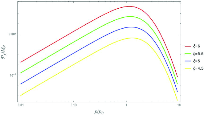
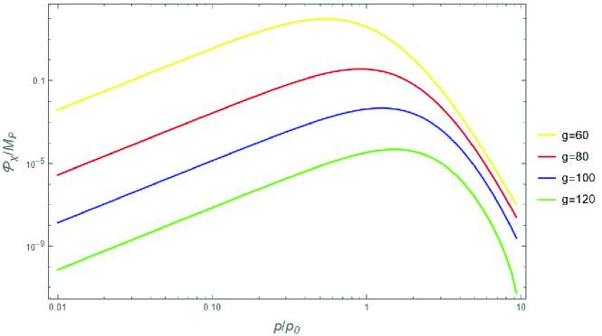
where . Based on numerical calculations Yu et al. (2023), we plot the power spectrum of the field for with varying values of and in Fig. 1. From the results, it is evident that is near , and specifically, larger and smaller yield higher . To match the CMB scale Mpc-1, we choose so that Mpc-1.
In the following we investigate the parameters and . We want that the induced GWs can be as large as possible. Therefore, we need to account for the backreaction of particle production on the evolution of the universe. As mentioned in Ref Yu et al. (2023), excessive particle production during inflation can terminate inflation prematurely, failing to provide sufficient e-folding to resolve the flatness problem. According to this condition, we can derive an upper limit on particle produced during inflation. For each value of , we can obtain a maximum value of . In Table. 1 we present maximum values of for the given values of . As expected, larger allows for larger , consistent with the earlier analysis.
| 20 | 40 | 60 | 80 | 100 | 120 | 140 | 160 | 180 | 200 | |
|---|---|---|---|---|---|---|---|---|---|---|
| 0.57 | 0.94 | 1.27 | 1.58 | 1.86 | 2.14 | 2.4 | 2.65 | 2.89 | 3.13 |
For our purpose, we need to identify the values of and which can induce the strongest GWs at the CMB scale. We calculate the energy spectrum of GWs at CMB scale Mpc-1. Since we only want to know the impact of induced GWs on the detection of primordial GWs, rough estimation of and is enough to get the appropriate parameters. We find can induce the strongest GWs at CMB scale Mpc-1.
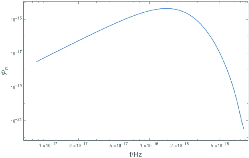
In Fig. 2,we present the resulting power spectrum of the GWs signal at the end of inflation. The spectrum features a peak around the CMB scale, consistent with our requirements. Through comparison with primordial GWs, we reveal that even the peak value is only about three thousandths of that of the primordial GWs. Therefore, if CMB B-mode polarization is detected and confirmed to be caused by GWs produced in the inflationary period, it would be straightforward to distinguish whether the source is quantum fluctuations or particle production in this way.
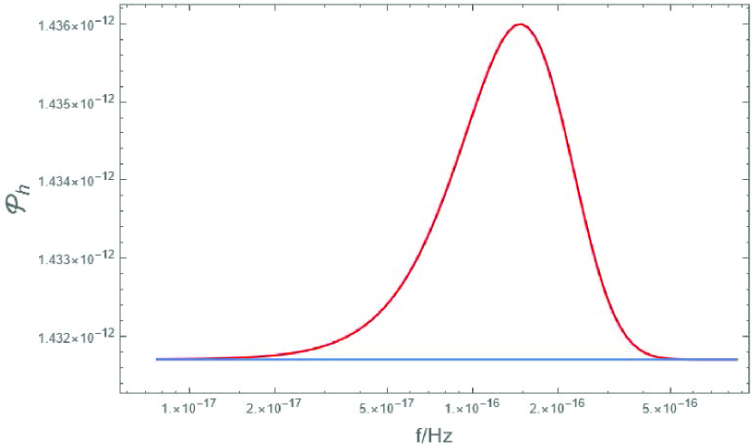
In Fig. 3, we show the total power spectrum of GWs including the standard primordial one and the particles induced one. A small additional peak appears in the scale-invariant spectrum of primordial GWs. This characteristic could be used to test the model and estimate values of the parameters. Additionally, we can also differentiate between primordial GWs and GWs induced by particle production in this way through it. Identifying inflationary tensor modes is crucial, as it provides the most promising avenue for extracting the energy scale of inflation and validating the standard consistency relation pertaining to the tensor-to-scalar ratio.
 |
IV Conclusion and discussion
In this paper, we examined the parameters governing particle production in the nonminimally coupled model and the gravitational waves (GWs) induced by the produced particles. The parameters and , which serve as coupling constants in this model, determine the duration over which particles are copiously produced. The parameter sets the time at which this process begins and influences the characteristic frequency of the scalar field . Then we verified these analyses by numerical calculations. Through the analysis of Eq. (2), we infer that induced GWs will feature a peak near the characteristic frequency of . By selecting an appropriate value for , we ensured that the induced GWs produced a peak close to the CMB scale, which allowed us to assess the impact of these particles on the detection of primordial GWs.
Taking into account the backreaction of particle production on inflation, we identified values for and that generate the strongest GWs at the CMB scale without violating the slow-roll mechanism. However, even for extreme values of and , the power spectrum of induced GWs only reaches about three thousandths of that of the primordial GWs at their peak. Therefore, if CMB B-mode polarization is detected and attributed to GWs from the inflationary period, it will be straightforward to distinguish whether these GWs originate from quantum fluctuations or from particle produced during inflation in this way.
The total power spectrum of GWs exhibits a distinct peak caused by particle production in the nonminimally coupled model. This feature provides a valuable tool for testing the model, estimating its parameters, and differentiating between primordial GWs and those induced by particle produced in this way. Identifying the origins of inflationary tensor modes remains critical, as it represents the most direct pathway to determining the energy scale of inflation and validating the consistency relation for the tensor-to-scalar ratio, offering profound insights into the physics of the early universe.
Acknowledgments
This work was supported in part by the National Key Research and Development Program of China Grant No. 2021YFC2203001 and in part by the NSFC (No. 12475046, No. 12375046, No. 12021003 and No. 12005016).
References
- Carlip et al. (2015) S. Carlip, D.-W. Chiou, W.-T. Ni, and R. Woodard, Int. J. Mod. Phys. D 24, 1530028 (2015), eprint 1507.08194.
- Kempf (2018) A. Kempf, Found. Phys. 48, 1191 (2018), eprint 1803.01483.
- Barrau (2017) A. Barrau, COMPTES RENDUS PHYSIQUE 18, 189 (2017), ISSN 1631-0705.
- Guzzetti et al. (2016a) M. C. Guzzetti, N. Bartolo, M. Liguori, and S. Matarrese, Riv. Nuovo Cim. 39, 399 (2016a), eprint 1605.01615.
- Guzzetti et al. (2016b) M. C. Guzzetti, N. Bartolo, M. Liguori, and S. Matarrese, RIVISTA DEL NUOVO CIMENTO 39, 399 (2016b), ISSN 0393-697X.
- Melia (2023) F. Melia, ASTROPARTICLE PHYSICS 152 (2023), ISSN 0927-6505.
- Shiraishi et al. (2016) M. Shiraishi, C. Hikage, R. Namba, T. Namikawa, and M. Hazumi, Phys. Rev. D 94, 043506 (2016), eprint 1606.06082.
- Moncelsi et al. (2020) L. Moncelsi et al., Proc. SPIE Int. Soc. Opt. Eng. 11453, 1145314 (2020), eprint 2012.04047.
- Dahal et al. (2020) S. Dahal et al., J. Low Temp. Phys. 199, 289 (2020), eprint 1908.00480.
- Suzuki et al. (2016) A. Suzuki et al. (POLARBEAR), J. Low Temp. Phys. 184, 805 (2016), eprint 1512.07299.
- Ade et al. (2019) P. Ade et al. (Simons Observatory), JCAP 02, 056 (2019), eprint 1808.07445.
- Liu et al. (2022) J. Liu, Z. Sun, J. Han, J. Carron, J. Delabrouille, S. Li, Y. Liu, J. Jin, S. Ghosh, B. Yue, et al., SCIENCE CHINA-PHYSICS MECHANICS & ASTRONOMY 65 (2022), ISSN 1674-7348.
- Abazajian et al. (2022) K. Abazajian et al. (CMB-S4), Astrophys. J. 926, 54 (2022), eprint 2008.12619.
- Krauss (1992) L. M. Krauss, Phys. Lett. B 284, 229 (1992).
- Caprini et al. (2016) C. Caprini et al., JCAP 04, 001 (2016), eprint 1512.06239.
- Wang et al. (2023) B.-R. Wang, J. Li, and H. Wang, Eur. Phys. J. C 83, 1010 (2023), eprint 2211.10617.
- Baumann and Zaldarriaga (2009) D. Baumann and M. Zaldarriaga, JCAP 06, 013 (2009), eprint 0901.0958.
- Krauss et al. (2010) L. M. Krauss, K. Jones-Smith, H. Mathur, and J. Dent, Phys. Rev. D 82, 044001 (2010), eprint 1003.1735.
- Yu et al. (2023) Z. Yu, C. Fu, and Z.-K. Guo, Phys. Rev. D 108, 123509 (2023), eprint 2307.03120.
- Starobinsky (1980) A. A. Starobinsky, Phys. Lett. B 91, 99 (1980).