6.5pt0.5pt

A three-family supersymmetric Pati-Salam model from rigid intersecting D6-branes

Abstract

We for the first time construct a three-family ${\cal N}=1$ supersymmetric Pati-Salam model from rigid intersecting D6-branes on a factorizable $\mathbb{T}^{6}/(\mathbb{Z}_{2}\times\mathbb{Z}_{2}^{\prime})$ orientifold with discrete torsion. We can break the Pati-Salam gauge symmetry down to the Standard Model (SM) gauge symmetry via the supersymmetry preserving Higgs mechanism, generate the SM fermion masses and mixings, and break the supersymmetry via gaugino condensations in the hidden sector.

Introduction – A great challenge in string phenomenology has been to construct the realistic string vacua, which can give the low energy supersymmetric Standard Models (SMs) without exotic particles, and stabilize the moduli fields. We can connect such string models to the low energy realistic particle physics via renormalization group equation running, and thus probe these models at the Large Hadron Collider (LHC) and the future Colliders, etc. We would like to emphasize that the semi-realistic supersymmetric Standard-like models and Grand Unified Theories (GUTs) have been constructed extensively in Type IIA theory on the $\mathbf{T^{6}/(\mathbb{Z}_{2}\times\mathbb{Z}_{2})}$ orientifold [1, 2, 3, 4, 5, 6, 7, 8, 9, 10, 11, 12, 13, 14, 15, 16, 17, 18, 19, 20, 21]. The key point is that only the Pati-Salam like models can explain all the Yukawa couplings [4]. The three family supersymmetric Pati-Salam models have been constructed systematically first in [4]. The SM fermion masses and mixings in some models have been explained explicitly [9, 10, 14, 19]. In particular, a systematic method was proposed to construct all the three-family ${\cal N}=1$ supersymmetric Pati-Salam models where the Pati-Salam gauge symmetry can be broken down to the SM gauge symmetry via the D-brane splitting and supersymmetry preserving Higgs mechanism [11, 12]. However, in these semi-realistic models, there exist three adjoint multiplets for $\textrm{U}(N)$ gauge symmetries since the D6-branes are not rigid. And the models from the rigid intersecting D6-branes are still very far from realistic [22, 23, 24, 25, 26, 27, 28, 29, 30]. Therefore, how to construct the three-family ${\cal N}=1$ supersymmetric Pati-Salam models from rigid intersecting D6-branes is a big challenge.

In Ref. [22] it was first shown that the global ${\cal N}=1$ chiral models can be constructed from the rigid intersecting D6-branes on a factorizable $\mathbb{T}^{6}/(\mathbb{Z}_{2}\times\mathbb{Z}_{2}^{\prime})$ orientifold with discrete torsion. However, the consistent three-generation models in this setup with factorizable tori were very difficult to engineer, and the examples in [22] generically had four generations. In the case of non-rigid branes, we need at least one torus to be tilted to generate three-generation models on the mirror orbifold $\mathbb{T}^{6}/(\mathbb{Z}_{2}\times\mathbb{Z}_{2})$ [1, 2, 3, 4, 5, 6, 7, 8, 9, 10, 11, 12, 13, 14, 15, 16, 17, 18, 19]. However, in the present setup with rigid 3-cycles, no consistent three-generation models employing tilted-tori are known. In Ref. [23] a first example of a three-generation model was indeed presented, however it was constructed on non-factorizable tori. The equivalent model with factorizable tori does not satisfy ${\cal N}=1$ supersymmetry conditions. In this letter, we for the first time construct a three-family ${\cal N}=1$ supersymmetric Pati-Salam model with factorizable tori from rigid intersecting D6-branes on a factorizable $\mathbb{T}^{6}/(\mathbb{Z}_{2}\times\mathbb{Z}_{2}^{\prime})$ orientifold, and briefly study its phenomenological consequences.

Model Building from Rigid Intersecting D6-Branes – Discrete torsion leads to rigid D6-branes wrapping fractional, and exceptional three-cycle collapsed to a lower dimensional fixed cycle in the orbifold limit of the Calabi-Yau space [24]. As the D6-branes are rigid, adjoint moduli disappear from the open string spectra: the irregularity of gauge symmetry breaking is removed along the flat direction, and one-loop beta functions are improved. Rigid branes allow instanton contributions to the Kähler potential, and superpotential generating $\mu$-terms [25], non-perturbative neutrino masses [26, 27], forbidden Yukawa couplings [28, 29] or might even trigger supersymmetry breaking [30].

In setup [22], the six-torus is factorizable as $\mathbb{T}^{6}=\mathbb{T}^{2}\times\mathbb{T}^{2}\times\mathbb{T}^{2}$, and the orbifold group is $\mathbb{Z}_{2}\times\mathbb{Z}^{\prime}_{2}$, where each $\mathbb{Z}_{2}$-factor inverts two two-tori. In addition to the untwisted cycles, there are 48 independent collapsed three-cycles from the twisted sectors. Thus, in this setup, there are, in total, 104 3-cycles, i.e., $b_{3}(\mathbb{T}^{6}/(\mathbb{Z}_{2}\times\mathbb{Z}_{2}^{\prime}))=2+2h^{21}_{unt}+2h^{21}_{tw}$, with $(h^{21}_{unt},h^{21}_{tw})=(3,48)$. For each sector, we denote the 16 fixed points on $(\mathbb{T}^{2}_{1}\times\mathbb{T}^{2}_{2})/\mathbb{Z}_{2}$ by $[e^{g}_{i,j}]$, with $g\in\{\Theta,\Theta^{\prime},\Theta\Theta^{\prime}\}$, and $i,j\in\{1,2,3,4\}$ as depicted in Fig. 1. After blowing up the orbifold singularities, these become two-cycles with the topology of $\mathbb{S}^{2}$. Each such four-dimensional $\mathbb{T}^{4}/\mathbb{Z}_{2}$ is an orbifold of $\mathbb{K}$3 before taking the other elements of the orientifold group into account. There are three $\mathbb{Z}_{2}$-twisted sectors with sixteen fixed points each. The three two-tori have radii $R_{1,2}^{(i)}$ along the $x^{i},y^{i}$-axes, $i\in\{1,2,3\}$. The tori may ($\beta^{i}=1$) or may not ($\beta^{i}=0$) be tilted. There are four orbifold fixed points on each torus, at $(0,0)$, $(0,R_{2}^{(i)}/2)$, $(R_{1}^{(i)}/2,\beta^{i}R_{2}^{(i)}/4)$ and $(R_{1}^{(i)}/2,(2+\beta^{i})R_{2}^{(i)}/4)$. They will be labelled fixed points $1,2,3$ and $4$. All this geometrical data is shown in Fig. 1 for an untilted and a tilted torus. The orientifold group is $\Omega{\cal R}(-1)^{F_{L}}$, where $F_{L}$ is the left-moving spacetime fermion number, $\Omega$ is world-sheet parity, and ${\cal R}$ is an isometric antiholomorphic involution of internal space acting on the Kähler class $J$ and three-from $\Omega_{3}$ as

$${\cal R}J=-J,\ \ {\cal R}\Omega_{3}=e^{2i\phi}\bar{\Omega}_{3},$$ (1)

with $\phi$ being real. The ${\cal R}$ can be thought of as complex conjugation if $\phi$ is vanishing. This gives rise to the orientifold plane at the fixed locus of ${\cal R}$. The branes (split into fractional branes) from hidden sector [32] are utilized in this letter to cancel the untwisted tadpoles.

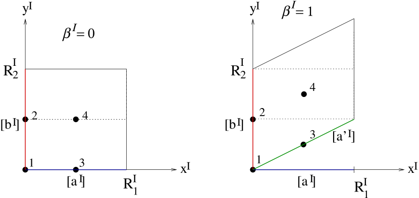
Figure 1: The $\mathbb{Z}_{2}$ invariant a-type (left) and b-type (right) lattices. $\mathbb{Z}_{2}$ fixed points are depicted in dots. The ${\cal R}$ invariant $x^{I}$ axis is along the 1-cycle $[a^{I}]-\frac{\beta^{I}}{2}[b^{I}]$ with $\beta^{I}=0$ for the a-type lattice and $\beta^{I}=1$ for the b-type lattice. ${\cal R}$ acts as reflection along the $y^{I}$ axis, which is spanned by the 1-cycle $[b^{I}]$. For the a-type lattice, all $\mathbb{Z}_{2}$ fixed points are invariant under ${\cal R}$, whereas for the b-type lattice, only 1 and 2 are invariant while 3 and 4 exchange as $3\stackrel{{\scriptstyle\cal R}}{{\leftrightarrow}}4$.

The (stacks of) D6-branes on this background are described by the wrapping numbers $(n^{i},m^{i})$, the charges under the twisted RR-fields $\epsilon^{i}\in\{-1,1\}$, the position $\delta^{i}\in\{0,1\}$, and the discrete Wilson lines $\lambda^{i}\in\{0,1\}$. The D6-brane wraps the one-cycle $n^{i}[{a^{\prime}}^{i}]+m^{i}[b^{i}]$ on the $i$-th torus, the fundamental one-cycles $[{a^{\prime}}^{i}]=[a^{i}]+\frac{\beta^{i}}{2}[b^{i}]$ and $[b^{i}]$ are shown in Fig. 1. The $\epsilon^{i}$ satisfy $\epsilon^{1}=\epsilon^{2}\epsilon^{3}$, and are related to the discrete Wilson lines [33]. The position is described by the three parameters $\delta^{i}$, where $\delta^{i}=0$ if the D6-brane goes through fixed point 1 on the $i$-th torus, and $\delta^{i}=1$ otherwise. An alternative way to characterise a D6-brane is to use $\epsilon^{i}_{kl}\in\{-1,0,1\}$, $i\in\{1,2,3\}$, $k,l\in\{1,2,3,4\}$ [22], instead of $\epsilon^{i}$, $\delta^{i}$ and $\lambda^{i}$. $\epsilon^{i}_{kl}$ is the charge of the D6-brane under the fixed point labelled $kl$ in the $i$-th twisted sector. The $\epsilon^{i}_{kl}$ can be determined from $\epsilon^{i}$, $\delta^{i}$ and $\lambda^{i}$. Note that for each $i$ only four out of the sixteen $\epsilon^{i}_{kl}$ are non-zero. In both these descriptions there is some redundancy [22]. Rather than fixing some of the $\epsilon^{i}_{kl}$ charges to be 1 [22], it will here be more convenient to choose $n^{1,2}>0$ (or $m^{i}$ positive if $n^{i}$ vanishes).

It is useful to define $\widetilde{m}^{i}=m^{i}+\frac{\beta^{i}}{2}n^{i}$, such that a D6-brane wraps the one-cycle $n^{i}[a^{i}]+\widetilde{m}^{i}[b^{i}]$ on the $i$-th torus. The volume of this one-cycle is given by

$$V^{i}=\sqrt{(n^{i})^{2}(R_{1}^{(i)})^{2}+(\widetilde{m}^{i})^{2}(R_{2}^{(i)})^{2}}~,~\,$$ (2)

and the tree-level gauge coupling is

$$\frac{1}{g_{\rm tree}^{2}} =e^{-\phi_{10}}\prod_{i}V^{i}=\frac{e^{-\phi_{4}}}{(T_{1}T_{2}T_{3})^{1/2}}\prod_{i}V^{i}$$

$$=\frac{(SU_{1}U_{2}U_{3})^{1/4}}{(T_{1}T_{2}T_{3})^{1/2}}\prod_{i}V^{i}\,$$ (3)

where $\phi_{10}$($\phi_{4}$) is the 10(4)-dimensional dilaton in string frame, $S$ is the dilaton in Einstein frame, $U_{i}$ are the (real parts of the) complex structure moduli in Einstein frame, and $T_{i}=R_{1}^{(i)}R_{2}^{(i)}$ are the (real parts of the) Kähler moduli. From (3) one can, using the supersymmetry condition (see below), derive the dependence of the tree-level gauge kinetic function on the untwisted moduli [34]

$$\hat{f}_{\rm tree}=S^{c}n^{1}n^{2}n^{3}-\sum_{i\neq j\neq k=1}^{3}U_{i}^{c}n^{i}\widetilde{m}^{j}\widetilde{m}^{k}\,,$$ (4)

where $S^{c}$ and $U_{i}^{c}$ are the complexified dilaton and complex structure moduli, the axions being RR-fields. Similarly, $T^{c}_{i}$ are complexified Kähler moduli with the axions stemming from the NSNS 2-form-field.

Sector	Representation
$aa$	${\rm U}(N_{a}/2)$ vector multiplet
	3 adjoint chiral multiplets
$ab+ba$	$I_{ab}\,(\yng(1)_{a},\overline{\yng(1)}_{b})=\Pi_{a}\circ\Pi_{b}$
$ab^{\prime}+b^{\prime}a$	$I_{ab^{\prime}}\,(\yng(1)_{a},\yng(1)_{b})=\Pi_{a}\circ\Pi_{b}^{\prime}$
$aa^{\prime}+a^{\prime}a$	$n_{\yng(2)}=\frac{1}{2}(\Pi_{a}\circ\Pi_{a}^{\prime}-\Pi_{a}\circ\Pi_{O6})$
	$n_{\yng(1,1)}=\frac{1}{2}(\Pi_{a}\circ\Pi_{a}^{\prime}+\Pi_{a}\circ\Pi_{O6})$

Table 1: Chiral spectrum for intersecting D6-branes at angles. Positive intersection numbers refer to the left-handed fermions.

The D6-brane is rotated by the angles $\theta^{i}$, defined via $\tan\theta^{i}=\widetilde{m}^{i}R_{2}^{(i)}/n^{i}R_{1}^{(i)}$, with respect to the x-axes of the three tori. Only supersymmetric configurations will be considered in this letter as

$$\sum_{i=1}^{3}\theta^{i}=0\mod 2\pi~.~\,$$ (5)

The charges of the four orientifold planes are denoted as $\eta_{\Omega{\cal R}}$ and $\eta_{\Omega{\cal R}i}$ with $i\in\{1,2,3\}$, and have to satisfy

$$\eta_{\Omega{\cal R}}\prod_{i=1}^{3}\eta_{\Omega{\cal R}i}=-1$$ (6)

in the present case of the $\mathbb{Z}_{2}\times\mathbb{Z}^{\prime}_{2}$ orbifold with $h_{21}=51$ [35, 22]. The tadpole cancellation conditions are given by

$$\sum_{a}N_{a}n_{a}^{1}n_{a}^{2}n_{a}^{3}=16\eta_{\Omega{\cal R}},$$

$$\sum_{a}N_{a}n_{a}^{i}\widetilde{m}_{a}^{j}\widetilde{m}_{a}^{k}=-2^{4-\beta^{j}-\beta^{k}}\eta_{\Omega{\cal R}i},~i\neq j\neq k\in\{1,2,3\},$$

$$\sum_{a}N_{a}n_{a}^{i}(\epsilon_{a,kl}^{i}-\eta_{\Omega{\cal R}}\eta_{\Omega{\cal R}i}\epsilon_{a,{\cal R}(k){\cal R}(l)}^{i})=0,$$

$$\sum_{a}N_{a}\widetilde{m}_{a}^{i}(\epsilon_{a,kl}^{i}+\eta_{\Omega{\cal R}}\eta_{\Omega{\cal R}i}\epsilon_{a,{\cal R}(k){\cal R}(l)}^{i})=0,$$ (7)

where ${\cal R}(k)=k$ in case of an untilted torus and ${\cal R}(\{1,2,3,4\})=\{1,2,4,3\}$ in the other case [22], and the sum is a sum over all stacks of D6-branes. $N_{a}$ denotes the number of D6-branes on stack $a$. The wrapping numbers and twisted charges carry an index $a$ denoting the D6-brane stack which they describe. The orientifold projection acts on the wrapping numbers and twisted charges as follows

$$\widetilde{m}^{I} \rightarrow -\widetilde{m}^{I}\,,$$ (8)

$$\epsilon_{kl}^{i} \rightarrow -\eta_{\Omega{\cal R}}\eta_{\Omega{\cal R}i}\epsilon^{i}_{{\cal R}(k){\cal R}(l)}\,.$$ (9)

Three-family ${\cal N}=1$ supersymmetric Pati-Salam models from rigid intersecting D6-branes – To construct the three family Pati-Salam model using rigid, semi-rigid and non-rigid branes, we follow the strategy outlined in [23]. In the $\mathbb{Z}_{2}\times\mathbb{Z}_{2}^{\prime}$ orbifold, the fractional branes invariant under $\Omega{\cal R}$ are those placed on top of an exotic O$6^{(+,+)}$ plane that is taken as O_ΩR in our choice (6). The adjoint fields from $aa$ sector do not arise due to the rigid D6-branes.

We present the model in Table 2, and the corresponding particle spectrum (only for pure rigid branes) in Table 4. The fixed points are given in Table 3 to produce the chiral spectrum, while the complete spectrum is presented in [32]. The additional constraint from (7) makes it very difficult to construct the consistent vacua that we could merely report a few more models in [32]. Indeed, the model reported in 2 is of phenomenological interest due to the breaking of the Pati-Salam gauge symmetry down to the SM gauge symmetry.

The purpose of the present section is to give an example of these more involved constructions which also admit the low energy theories very closer to realistic particle physics. Models presented in [32] usually do not have the Higgs fields to break the Pati-Salam gauge symmetry down to the SM. We address this important feature of model building for the Model in Table 2. With the choice of the fixed points listed in Table 3, one can calculate the chiral spectrum presented in Table 4. The Table 2 consists of five sets D6-branes, i.e., ${a,b,c,d,e}$. The set $a$ consists of five stacks of fractional D6-branes, but each with different bulk wrapping numbers. The set $a$, most importantly, gives rise to the gauge symmetries and chiral spectrum. In contrast to the set $a$, the sets $b$, $c$, $d$, and $e$ are the bulk the D6-branes which are split into fractional constituents. It can be checked that The table 2 satisfies all the constraints presented in (7) for untwisted and twisted tadpoles, and (5) for supersymmetry condition.

The gauge symmetries derived from the set $a$ are $\textrm{SU}(4)\times\textrm{SU}(2)_{L}\times\textrm{SU}(2)_{1}\times\textrm{SU}(2)_{2}\times\textrm{USp}(4)$, which give rise to the Pati-Salam-like theory from the subsets $a_{1}$, $a_{2}$, $a_{3}$, and $a_{4}$. In contrast to set $a$, the sets $b$, $c$, $d$, and $e$ yield the gauge symmetries $\textrm{USp}(4)^{4}$, $\textrm{U}(2)^{2}$, $\textrm{U}(4)^{2}$, and $\textrm{U}(4)^{2}$, respectively. The latter gauges groups from the fractional D6-branes can be deformed into bulk D6-branes upon Higgsings as follows

$$\{b_{1},b_{2},b_{3},b_{4}\},\{c_{1},c_{2}\},\{d_{1},d_{2}\},\{e_{1},e_{2}\}\to b,c,d,e$$ (10)

$$\textrm{USp}(4)^{4}\times\textrm{U}(2)^{2}\times\textrm{U}(4)^{2}\times\textrm{U}(4)^{2}\to\textrm{USp}(4)\times\textrm{U}(1)\times\textrm{U}(2)\times\textrm{U}(2).$$ (11)

Some of the $\textrm{U}(1)$s are not really gauge symmetries, but only global ones because their gauge bosons would receive Stueckelberg mass through the Green-Schwarz mechanism [2]. Thus, Pati-Salam gauge symmetries $\textrm{SU}(4)\times\textrm{SU}(2)\times\textrm{SU}(2)$ are obtained from D-branes $a_{1}$, $a_{2}$, $a_{3}$, and $a_{4}$, while the extra symmetries $\textrm{USp}(4)^{4}\times\textrm{U}(2)^{2}\times\textrm{U}(4)^{2}\times\textrm{U}(4)^{2}$ arise from the set $b$, $c$, $d$, and $e$ which turns out to be, after Higgsing (11), the gauge symmetries $\textrm{USp}(4)\times\textrm{U}(1)\times\textrm{U}(2)\times\textrm{U}(2)$.

$\begin{array}[]{|c|c|c|}\hline\cr{\rm Stack}&N&(n^{1},m^{1})\times(n^{2},m^{2})\times(n^{3},m^{3})\\ \hline\cr\hline\cr a_{1}&4&(0,1)\times(1,0)\times(0,-1)\\ a_{2}&2&(-4,-1)\times(-2,1)\times(1,0)\\ a_{3}&2&(4,1)\times(2,1)\times(-3,-1)\\ a_{4}&2&(-1,0)\times(-2,1)\times(2,1)\\ a_{5}&2&(1,0)\times(0,1)\times(0,-1)\\ \hline\cr b_{1}&2&(1,0)\times(1,0)\times(1,0)\\ b_{2}&2&(-1,0)\times(-1,0)\times(1,0)\\ b_{3}&2&(1,0)\times(-1,0)\times(-1,0)\\ b_{4}&2&(-1,0)\times(1,0)\times(-1,0)\\ \hline\cr c_{1}&2&(1,0)\times(0,-1)\times(0,1)\\ c_{2}&2&(-1,0)\times(0,1)\times(0,1)\\ \hline\cr d_{1}&4&(0,-1)\times(1,0)\times(0,1)\\ d_{2}&4&(0,1)\times(-1,0)\times(0,1)\\ \hline\cr e_{1}&4&(0,-1)\times(0,1)\times(1,0)\\ e_{2}&4&(0,-1)\times(0,-1)\times(-1,0)\\ \hline\cr\end{array}$

Table 2: Model with gauge symmetries $\textrm{SU}(4)_{C}\times\textrm{SU}(2)_{L}\times\textrm{SU}(2)_{1}\times\textrm{SU}(2)_{2}\times\textrm{SU}(2)^{3}\times\textrm{USp}(4)^{4}\times\textrm{SU}(4)^{4}$. The torus moduli are $\chi_{1}=8$, $\chi_{2}=4$, $\chi_{3}=3$, and the tree-level gauge coupling relation is $g_{C}^{2}=\frac{5}{4}g_{L}^{2}=\frac{25}{44}g_{R}^{2}=\frac{125}{182}\frac{5}{3}g_{Y}^{2}=2\sqrt{2}\pi e^{\phi_{4}}$.

Unlike the previous construction [32], the rigid brane $a_{4}$ is moved into visible sector for the sake of symmtery breaking, thus modifying the condition for three generations,

$$I_{a_{1}a_{2}}+I_{a_{1}a_{2}^{\prime}}=\pm 3,$$ (12)

$$I_{a_{1}a_{3}}+I_{a_{1}a_{3}^{\prime}}+I_{a_{1}a_{4}}+I_{a_{1}a_{4}^{\prime}}=\mp 3.$$ (13)

We present the chiral spectrum of this theory in the Table 4. In particular, we present the conventions of some particles concretely, for example, the SM fermions, and Higgs fields, etc. Moreover, the visible sector will suffer from the uncancelled twisted tadpoles. Therefore, an additional D6-brane $a_{5}$ is added to cancel the latter. In order to get the consistent model, untwisted tadpoles are canceled by adding more semi-rigid branes from the set $b$, $c$, $d$, and $e$ such that they do not make any contribution to the twisted tadpoles.

$\begin{array}[]{|c|c|c|c|}\hline\cr\text{Cycles}&\text{$\Theta$-sector}&\text{$\Theta^{\prime}$-sector}&\text{$\Theta\Theta^{\prime}$-sector}\\ \hline\cr\Pi_{a_{1}}&\{\{1,2\},\{1,3\}\}&\{\{1,3\},\{1,2\}\}&\{\{1,2\},\{1,2\}\}\\ \hline\cr\Pi_{a_{2}}&\{\{1,2\},\{1,2\}\}&\{\{1,2\},\{1,3\}\}&\{\{1,2\},\{1,3\}\}\\ \hline\cr\Pi_{a_{3}}&\{\{1,2\},\{1,2\}\}&\{\{1,2\},\{1,4\}\}&\{\{1,2\},\{1,4\}\}\\ \hline\cr\Pi_{a_{4}}&\{\{1,3\},\{1,2\}\}&\{\{1,2\},\{1,2\}\}&\{\{1,3\},\{1,2\}\}\\ \hline\cr\Pi_{a_{5}}^{*}&\{\{2,4\},\{3,4\}\}&\{\{3,4\},\{3,4\}\}&\{\{2,4\},\{3,4\}\}\\ \hline\cr\Pi_{b}^{*}&\{\{2,4\},\{2,4\}\}&\{\{2,4\},\{2,4\}\}&\{\{2,4\},\{2,4\}\}\\ \hline\cr\Pi_{c}^{*}&\{\{2,4\},\{3,4\}\}&\{\{3,4\},\{3,4\}\}&\{\{2,4\},\{3,4\}\}\\ \hline\cr\Pi_{d}&\{\{1,2\},\{1,3\}\}&\{\{1,3\},\{1,2\}\}&\{\{1,2\},\{1,2\}\}\\ \hline\cr\Pi_{e}^{*}&\{\{3,4\},\{3,4\}\}&\{\{3,4\},\{2,4\}\}&\{\{3,4\},\{2,4\}\}\\ \hline\cr\end{array}$

Table 3: The D6-branes with asteric move away from the orgin, while the rest of D6-branes pass through the origin. As the bulk branes turned into fractional branes pass through the same set of fixed points, they are written in compact notaion, i.e., $\Pi_{b}$, $\Pi_{c}$, and $\Pi_{d}$.

Phenomenological Study – The gauge symmetries from $a_{1}$, $a_{2}$, $a_{3}$, and $a_{4}$ are $\textrm{U}(4)_{C}$, $\textrm{U}(2)_{L}$, $\textrm{U}(2)_{1}$, and $\textrm{U}(2)_{2}$, respectively. The anomalies from four global $\textrm{U}(1)$s of $\textrm{U}(4)_{C}$, $\textrm{U}(2)_{L}$, $\textrm{U}(2)_{1}$, and $\textrm{U}(2)_{2}$ are cancelled by the Green-Schwarz mechanism, and the gauge fields of these $\textrm{U}(1)$s obtain masses via the linear $B\wedge F$ couplings. So, the effective gauge symmetry is $\textrm{SU}(4)_{C}\times\textrm{SU}(2)_{L}\times\textrm{SU}(2)_{1}\times\textrm{SU}(2)_{2}$. When $\Delta_{i}$ obtain Vacuum Expectation Values (VEVs), the $\textrm{SU}(2)_{1}\times\textrm{SU}(2)_{2}$ gauge symmetry is broken down to the diagonal $\textrm{SU}(2)_{R}$ gauge symmetry. Thus, we obtain the Pati-Salam $\textrm{SU}(4)_{C}\times\textrm{SU}(2)_{L}\times\textrm{SU}(2)_{R}$ gauge symmetry. We have three families of left-handed fermions $F^{i}$, and three families of right-handed fermions from $F_{R}^{i}$, $F_{R}^{c}$, $F_{R}^{\prime ci}$, i.e., $6-1-2=3$. Moreover, by giving VEVs to $F_{R}^{c}$ and a linear combination of $F_{R}^{i}$, we can break the Pati-Salam gauge symmetry down to the SM gauge symmetry and preserve the four-dimensional ${\cal N}=1$ supersymmetry by keeping the D-flatness and F-flatness. In addition, we can generate the SM fermion masses and mixing, as well as the vector-like particle masses for $F_{R}^{\prime ci}$ and two other linear combinations of $F_{R}^{i}$ via the following superpotential

$$W\supset y_{ij}^{k}F_{L}^{i}F_{R}^{j}\Phi_{k}+y_{ij}^{\prime k}F_{R}^{\prime ci}F_{R}^{j}\Delta_{k}\,.$$ (14)

Furthermore, the $\textrm{SU}(4)$ gauge symmetries in the hidden sector have negative beta functions, and then the supersymmetry can be broken via gaugino condensations.

$\begin{array}[]{|c|r|}\hline\cr{\rm Sector}&\textrm{SU}(4)\times\textrm{SU}(2)_{L}\times\textrm{SU}(2)_{1}\times\textrm{SU}(2)_{2}\times{\rm Hidden}\\ \hline\cr a_{1}a_{2}&F^{i}_{L}(Q_{L},L_{L}):~3\times\left(4,\bar{2},1,1,1,1,1,1,1,1,1,1,1,1,1\right)\\ a_{1}a_{3}^{\prime}&F^{i}_{R}(Q_{R},L_{R}):~6\times\left(\bar{4},1,\bar{2},1,1,1,1,1,1,1,1,1,1,1,1\right)\\ a_{1}a_{3}&F^{c}_{R}(Q_{R},L_{R}):~1\times\left(4,1,\bar{2},1,1,1,1,1,1,1,1,1,1,1,1\right)\\ a_{1}a_{4}&F^{\prime ic}_{R}(Q_{R},L_{R}):~2\times\left(4,1,1,\bar{2},1,1,1,1,1,1,1,1,1,1,1\right)\\ a_{2_{\overline{\yng(1,1)}}}&S_{L}^{i}:~4\times(1,\bar{1}_{\overline{\yng(1,1)}},1,1,1,1,1,1,1,1,1,1,1,1,1)\\ a_{2}a_{3}&\Phi^{\prime}_{i}(H^{\prime}_{u},H^{\prime}_{d}):~3\times\left(1,\bar{2},2,1,1,1,1,1,1,1,1,1,1,1,1\right)\\ a_{2}a_{3}^{\prime}&\Phi_{i}(H_{u}^{i},H_{d}^{i}):~5\times\left(1,2,2,1,1,1,1,1,1,1,1,1,1,1,1\right)\\ a_{2}a_{4}^{\prime}&1\times\left(1,2,1,2,1,1,1,1,1,1,1,1,1,1,1\right)\\ a_{3_{\overline{\yng(2)}}}&T_{R}^{i}:~6\times(1,1,\bar{3}_{\overline{\yng(2)}},1,1,1,1,1,1,1,1,1,1,1,1)\\ a_{3_{\overline{\yng(1,1)}}}&S_{R}^{i}:~60\times(1,1,\bar{1}_{\overline{\yng(1,1)}},1,1,1,1,1,1,1,1,1,1,1,1)\\ a_{3}a_{4}^{\prime}&\Delta_{i}:~3\times\left(1,1,2,2,1,1,1,1,1,1,1,1,1,1,1\right)\\ \hline\cr\end{array}$

Table 4: The chiral particle spectrum for model in Table 2, and the hidden part of symmetry is $\textrm{SU}(2)^{3}\times\textrm{USp}(4)^{4}\times\textrm{SU}(4)^{4}$. The chiral spectrum is singlet under latter symmetry.

Conclusions – We have presented a three-generation ${\cal N}=1$ supersymmetric Pati-Salam models from rigid intersecting D6-branes on $\mathbb{T}^{6}/(\mathbb{Z}_{2}\times\mathbb{Z}_{2}^{\prime})$ orientifold with discrete torsion. The model is first of its kind constructed in the factorizable compactification lattice. The construction is particularly simple as it only involves rectangular two-tori. We showed that the Pati-Salam gauge symmetry can be broken down to the SM gauge symmetry via the supersymmetry preserving Higgs mechanism, the SM fermion masses and mixings can be generated, and the supersymmetry can be broken via gaugino condensations in the hidden sector. The detailed phenomenology of the model needs a thorough analysis of the gauge coupling unification, the supersymmetry breaking soft terms, and the allowed masses of the SM fermions with moduli stabilization, which will be explored in a future study.

References

- Cvetic et al. [2001a] M. Cvetic, G. Shiu, and A. M. Uranga, Three family supersymmetric standard - like models from intersecting brane worlds, Phys. Rev. Lett. 87, 201801 (2001a), arXiv:hep-th/0107143 .
- Cvetic et al. [2001b] M. Cvetic, G. Shiu, and A. M. Uranga, Chiral four-dimensional N=1 supersymmetric type 2A orientifolds from intersecting D6 branes, Nucl. Phys. B 615, 3 (2001b), arXiv:hep-th/0107166 .
- Cvetic et al. [2003] M. Cvetic, I. Papadimitriou, and G. Shiu, Supersymmetric three family SU(5) grand unified models from type IIA orientifolds with intersecting D6-branes, Nucl. Phys. B 659, 193 (2003), [Erratum: Nucl.Phys.B 696, 298–298 (2004)], arXiv:hep-th/0212177 .
- Cvetic et al. [2004] M. Cvetic, T. Li, and T. Liu, Supersymmetric Pati-Salam models from intersecting D6-branes: A Road to the standard model, Nucl. Phys. B 698, 163 (2004), arXiv:hep-th/0403061 .
- Blumenhagen et al. [2005a] R. Blumenhagen, M. Cvetic, P. Langacker, and G. Shiu, Toward realistic intersecting D-brane models, Ann. Rev. Nucl. Part. Sci. 55, 71 (2005a), arXiv:hep-th/0502005 .
- Chen et al. [2006a] C.-M. Chen, T. Li, and D. V. Nanopoulos, Standard-like model building on Type II orientifolds, Nucl. Phys. B 732, 224 (2006a), arXiv:hep-th/0509059 .
- Chen et al. [2006b] C.-M. Chen, T. Li, and D. V. Nanopoulos, Type IIA Pati-Salam flux vacua, Nucl. Phys. B 740, 79 (2006b), arXiv:hep-th/0601064 .
- Chen et al. [2006c] C.-M. Chen, T. Li, and D. V. Nanopoulos, Flipped and unflipped SU(5) as type IIA flux vacua, Nucl. Phys. B 751, 260 (2006c), arXiv:hep-th/0604107 .
- Chen et al. [2008a] C.-M. Chen, T. Li, V. E. Mayes, and D. V. Nanopoulos, A Realistic world from intersecting D6-branes, Phys. Lett. B 665, 267 (2008a), arXiv:hep-th/0703280 .
- Chen et al. [2008b] C.-M. Chen, T. Li, V. E. Mayes, and D. V. Nanopoulos, Towards realistic supersymmetric spectra and Yukawa textures from intersecting branes, Phys. Rev. D 77, 125023 (2008b), arXiv:0711.0396 [hep-ph] .
- He et al. [2022a] W. He, T. Li, R. Sun, and L. Wu, The final model building for the supersymmetric Pati–Salam models from intersecting D6-branes, Eur. Phys. J. C 82, 710 (2022a), arXiv:2112.09630 [hep-th] .
- He et al. [2022b] W. He, T. Li, and R. Sun, The complete search for the supersymmetric Pati-Salam models from intersecting D6-branes, JHEP 08, 044, arXiv:2112.09632 [hep-th] .
- Li et al. [2023] T. Li, R. Sun, and L. Wu, String-scale gauge coupling relations in the supersymmetric Pati-Salam models from intersecting D6-branes, JHEP 03, 210, arXiv:2212.05875 [hep-th] .
- Sabir et al. [2022] M. Sabir, T. Li, A. Mansha, and X.-C. Wang, The supersymmetry breaking soft terms, and fermion masses and mixings in the supersymmetric Pati-Salam model from intersecting D6-branes, JHEP 04, 089, arXiv:2202.07048 [hep-th] .
- Li et al. [2021a] T. Li, A. Mansha, and R. Sun, Revisiting the supersymmetric Pati–Salam models from intersecting D6-branes, Eur. Phys. J. C 81, 82 (2021a), arXiv:1910.04530 [hep-th] .
- Li et al. [2021b] T. Li, A. Mansha, R. Sun, L. Wu, and W. He, N=1 supersymmetric models, models, and models from intersecting D6-branes, Phys. Rev. D 104, 046018 (2021b).
- Mansha et al. [2024a] A. Mansha, T. Li, M. Sabir, and L. Wu, Three-family supersymmetric Pati–Salam models with symplectic groups from intersecting D6-branes, Eur. Phys. J. C 84, 151 (2024a), arXiv:2212.09644 [hep-th] .
- Mansha et al. [2023] A. Mansha, T. Li, and L. Wu, The hidden sector variations in the supersymmetric three-family Pati–Salam models from intersecting D6-branes, Eur. Phys. J. C 83, 1067 (2023), arXiv:2303.02864 [hep-th] .
- Sabir et al. [2024a] M. Sabir, A. Mansha, T. Li, and Z.-W. Wang, Fermion masses and mixings in the supersymmetric Pati-Salam landscape from Intersecting D6-Branes, JHEP 10, 252, arXiv:2409.09110 [hep-ph] .
- Sabir et al. [2024b] M. Sabir, A. Mansha, T. Li, and Z.-W. Wang, Susy breaking soft terms in the supersymmetric Pati-Salam landscape from Intersecting D6-Branes, (2024b), arXiv:2410.09093 [hep-ph] .
- Mansha et al. [2024b] A. Mansha, T. Li, and M. Sabir, Revisiting the supersymmetric trinification models from intersecting D6-branes, Commun. Theor. Phys. 76, 095201 (2024b), arXiv:2406.07586 [hep-th] .
- Blumenhagen et al. [2005b] R. Blumenhagen, M. Cvetic, F. Marchesano, and G. Shiu, Chiral D-brane models with frozen open string moduli, JHEP 03, 050, arXiv:hep-th/0502095 .
- Forste and Zavala [2008] S. Forste and I. Zavala, Oddness from Rigidness, JHEP 07, 086, arXiv:0806.2328 [hep-th] .
- Blumenhagen et al. [2002] R. Blumenhagen, V. Braun, B. Kors, and D. Lust, Orientifolds of K3 and Calabi-Yau manifolds with intersecting D-branes, JHEP 07, 026, arXiv:hep-th/0206038 .
- Ibanez and Richter [2009] L. E. Ibanez and R. Richter, Stringy Instantons and Yukawa Couplings in MSSM-like Orientifold Models, JHEP 03, 090, arXiv:0811.1583 [hep-th] .
- Blumenhagen et al. [2007] R. Blumenhagen, M. Cvetic, and T. Weigand, Spacetime instanton corrections in 4D string vacua: The Seesaw mechanism for D-Brane models, Nucl. Phys. B 771, 113 (2007), arXiv:hep-th/0609191 .
- Ibanez and Uranga [2007] L. E. Ibanez and A. M. Uranga, Neutrino Majorana Masses from String Theory Instanton Effects, JHEP 03, 052, arXiv:hep-th/0609213 .
- Abel and Goodsell [2007] S. A. Abel and M. D. Goodsell, Realistic Yukawa Couplings through Instantons in Intersecting Brane Worlds, JHEP 10, 034, arXiv:hep-th/0612110 .
- Blumenhagen et al. [2008] R. Blumenhagen, M. Cvetic, D. Lust, R. Richter, and T. Weigand, Non-perturbative Yukawa Couplings from String Instantons, Phys. Rev. Lett. 100, 061602 (2008), arXiv:0707.1871 [hep-th] .
- Cvetic and Weigand [2008] M. Cvetic and T. Weigand, A String theoretic model of gauge mediated supersymmetry beaking, (2008), arXiv:0807.3953 [hep-th] .
- Note [1] Unlike [22], we take and not 1/2 for the tilted torus.
- [32] A. Mansha, T. Li, M. Sabir, Three-family Pati-Salam models from rigid branes, in preparation.
- Sen [1998] A. Sen, Stable nonBPS bound states of BPS D-branes, JHEP 08, 010, arXiv:hep-th/9805019 .
- Lust et al. [2004] D. Lust, P. Mayr, R. Richter, and S. Stieberger, Scattering of gauge, matter, and moduli fields from intersecting branes, Nucl. Phys. B 696, 205 (2004), arXiv:hep-th/0404134 .
- Blumenhagen and Schmidt-Sommerfeld [2007] R. Blumenhagen and M. Schmidt-Sommerfeld, Gauge Thresholds and Kaehler Metrics for Rigid Intersecting D-brane Models, JHEP 12, 072, arXiv:0711.0866 [hep-th] .