LoRS: Efficient Low-Rank Adaptation for Sparse Large Language Model
Abstract
Existing low-rank adaptation (LoRA) methods face challenges on sparse large language models (LLMs) due to the inability to maintain sparsity. Recent works introduced methods that maintain sparsity by augmenting LoRA techniques with additional masking mechanisms. Despite these successes, such approaches suffer from an increased memory and computation overhead, which affects efficiency of LoRA methods. In response to this limitation, we introduce LoRS, an innovative method designed to achieve both memory and computation efficiency when fine-tuning sparse LLMs. To mitigate the substantial memory and computation demands associated with preserving sparsity, our approach incorporates strategies of weight recompute and computational graph rearrangement. In addition, we also improve the effectiveness of LoRS through better adapter initialization. These innovations lead to a notable reduction in memory and computation consumption during the fine-tuning phase, all while achieving performance levels that outperform existing LoRA approaches.
LoRS: Efficient Low-Rank Adaptation for Sparse Large Language Model
Yuxuan Hu1,2, Jing Zhang1,2††thanks: Corresponding author. zhang-jing@ruc.edu.cn, Xiaodong Chen1,2 Zhe Zhao4, Cuiping Li1,3, Hong Chen1,3 1School of Information, Renmin University of China, Beijing, China 2Key Laboratory of Data Engineering and Knowledge Engineering, Beijing, China 3Engineering Research Center of Database and Business Intelligence, Beijing, China 4Tencent AI Lab, Beijing, China
1 Introduction
Large language models (LLMs) Touvron et al. (2023b); Dubey et al. (2024) have demonstrated remarkable proficiency in numerous natural language processing tasks, which has spurred their increasing integration into diverse applications. However, the deployment of these models is constrained by their vast parameter counts, necessitating significant hardware resources that can be prohibitive for many users. Moreover, the large scale of LLMs can impede inference speed, presenting a challenge in scenarios requiring rapid response times.
To mitigate these issues, various post-training pruning methods have been introduced, such as SparseGPT Frantar and Alistarh (2023), Wanda Sun et al. (2024), and RIA Zhang et al. (2024). These techniques effectively reduce model parameters, transforming dense models into sparse versions with minimal data requirements and within short periods. Despite their efficiency, pruned models still exhibit a performance disparity compared to their original counterparts, especially in small and medium-sized models with unstructured or 2:4 semi-structured sparsity Mishra et al. (2021). This discrepancy limits the practical utility of pruned models. Continuous pre-training could help bridge this gap but comes at a high computational cost. Consequently, there is a pressing need for tuning methods that maintain sparsity while optimizing memory and parameter efficiency.
Low-Rank Adaptation (LoRA) Hu et al. (2021) was developed to ease the computational demands of training dense LLMs. LoRA enables fine-tuning with reduced resource consumption, making it widely applicable for dense models. Recent studies SPP Lu et al. (2024) and SQFT Munoz et al. (2024), have extended LoRA to accommodate sparse LLMs by incorporating masking mechanisms. We refer to these methods as Sparsity Preserved LoRA methods (SP-LoRA). SPP and SQFT achieving performance similar to LoRA, while ensuring the sparsity of the model. However, they increase computation and memory overhead, undermining LoRA’s inherent efficiency. Specifically, SQFT requires twice the memory overhead of LoRA, while SPP reduces the memory overhead to the same as LoRA through gradient checkpoints Chen et al. (2016), but greatly increases the time overhead.
In response to these limitations, we present an innovative Low Rank Adaptation method for Sparse LLM (LoRS). LoRS addresses the increased memory and computational overhead caused by masking mechanisms through weight recompute, and computational graph rearrangement. Our approach discards the fitness weights during each forward pass and recalculates them during backward passes, thereby significantly reducing the memory overhead at the cost of a small amount of additional computation. Meanwhile, we optimize the gradient computation by computation graph rearrangement in the backward pass, which further reduces the computational overhead compared to SQFT and SPP. In addition, inspired by the latest LoRA variants, we also improve the efficiency of LoRS by better adapter initialization.
We evaluate LoRS on multiple LLMs, initially pruning them via post-training methods like Wanda or SparseGPT. Subsequently, LoRS is used to fine-tune these models using instruction datasets or pretraining datasets. The zero-shot performance of the tuned sparse LLMs is then assessed across a variety of benchmark tasks. The main contributions of this paper are summarized in the following:
(1) We introduce LoRS, a novel fine-tuning method for sparse LLMs that preserves sparsity while minimizing computation and memory overhead. LoRS leverages weight recompute and computational graph rearrangement techniques to achieve this efficiency and achieve better performance through better adapter initialization.
(2) Through comprehensive experiments on sparse LLMs with different sparsity patterns, we show that LoRS can outperform existing SP-LoRA methods in terms of performance, memory usage, and computation efficiency.
2 LoRS
In this section, we begin by reviewing unstructured pruning and low-rank adaptation in Section 2.1. We then proceed to analyze the memory complexity associated with existing methods in Section 2.2. We then describe how our method LoRS optimizes the memory and computational overhead of existing methods in section 2.3. Finally, in Section 2.4, we describe how the performance of LoRS can be improved by better adapter initialization.
2.1 Preliminary
Unstructured Pruning. Unstructured pruning Frantar and Alistarh (2023); Sun et al. (2024); Zhang et al. (2024) converts dense weight matrices of LLMs into sparse matrices to enhance computational efficiency. Given the original dense weight matrix , pruning aims to produce a sparse matrix through the application of a binary mask and weight updates . This process is mathematically represented as: , where denotes element-wise multiplication. The mask zeros out less important weights, while fine-tunes the retained weights, ensuring that the pruned model preserves its performance.
LoRA. Low-Rank Adaptation Hu et al. (2021); Wang et al. (2024) is an efficient approach designed to fine-tune LLMs for specific tasks or domains by training only a limited set of parameters. This method allows the model to be adapted to specific tasks while significantly reducing computational cost.
The mathematical representation of LoRA is expressed as , where stands for the initial weight matrix of the pre-trained model. The term denotes the adapted weight matrix at the -th iteration of training. The matrices and represent the trainable adapter matrices at the -th iteration. Specifically, and , with being much smaller in dimension compared to and . Here, and represents the dimensions of the original weight matrix. In practice, during the adaptation process, only the parameters within and are updated, while all other parameters remain fixed. This strategy ensures that the model can be efficiently tuned to new tasks or domains without altering the entire pre-trained weights.
SP-LoRA. To maintain the sparsity of the model while adaptation, SP-LoRA methods Lu et al. (2024); Munoz et al. (2024) integrate a masking mechanism within the LoRA framework. Let us consider a sparse large language model (LLM) with a weight matrix and its associated mask . During each training iteration , the mask is applied to enforce the sparsity of the weight matrix, which can be mathematically represented as:
| (1) |
Here, denotes element-wise multiplication, while and represent adapter matrices that are updated at each iteration.
The incorporation of the mask, while ensuring that the weights remain sparse, modifies the computational graph of the original LoRA framework. This modification results in increased GPU memory usage and computation overhead, presenting practical challenges. Therefore, we will first investigate the reasons behind this elevated GPU memory and computation consumption, and subsequently propose an effective solution to mitigate this issue.
2.2 Complexity Analysis
At the -th training iteration, let us denote the input to the weight matrix as . For LoRA, the output can be mathematically represented as
| (2) |
The computation process unfolds in these steps:
where , , and represent intermediate activations with dimensions , , and respectively. During back-propagation, gradients for , , and are computed based on the gradient of , denoted as . The gradient computations are formulated as follows:
In the forward pass, the input and intermediate activation are stored for back-propagation, involving parameters. Meanwhile, the corresponding multiply–accumulate operations (MACs) for forward is and for backward is .
For SP-LoRA, the output expression modifies to
| (3) |
where acts as a mask indicating non-zero elements in . Unlike LoRA, SP-LoRA requires computing before multiplying by . This sequence of operations is outlined as:
Meanwhile, back-propagation for SP-LoRA involves:
SP-LoRA’s forward pass necessitates retaining , , and for back-propagation including parameters, and the MACs corresponding to the forward and backward are and , respectively.
Based on frequently used model sizes and training configurations, we assume that . Comparing LoRA and SP-LoRA, it can be seen that incorporating masks in SP-LoRA significantly raises GPU memory overhead due to traced mask and weight matrix in computational graph (). Meanwhile, SP-LoRA requires additional computation in the backward pass due to the need to compute the gradient of the weight matrix (). Therefore, optimizing GPU memory usage and computation overhead in SP-LoRA is essential.
In this work, we consider the most advanced SP-LoRA methods SPP and SQFT, where SQFT does not take into account the memory and computational overheads and has the same complexity as analyzed above. SPP, on the other hand, optimizes memory usage through PyTorch’s built-in gradient checkpoint API, and its implementation is shown in Appendix A. Thus, on top of LoRA, SPP reduces the number of parameters that need to be stored in the computational graph (), but introduces additional computation during backward pass ().
2.3 Memory and Computation Optimization
After comparing the computational processes of LoRA and SP-LoRA, it is evident that the memory overhead in SP-LoRA arises from the need to maintain additional masks and adapted weight matrices within the computational graph, and the computation overhead arises from the need to compute the gradient of weight matrices.
To address the memory overhead, inspired by gradient checkpoint Chen et al. (2016), we introduce weight recompute strategie in LoRS, effectively eliminating the necessity for masks and adapted weight matrices in the computation graph. Specifically, we release the intermediate weights and directly after the forward pass of the LoRS, and recompute them later during the backward pass. After optimization, only the input activation is saved to the computational graph for subsequent backward pass. With this optimization, for each linear layer, we reduce the recorded parameter from to , while only increasing the computational overhead of MACs.
After that, to reduce the computation overhead associated with computing the gradient of the weight matrix, we propose the computational graph reordering method. Firstly, we find that the masking operation of the gradient during backward pass () has minimal effect on the model performance and thus can be ignored, which is equivalent to estimating the gradient using straight through estimator Bengio et al. (2013); Zhou et al. (2021a). After that, we can directly compute gradients and based on , , , and , i.e.,
Instead of following the computational graph and prioritizing the computation of , we can reorder the computation process to compute and first, thus reducing the MACs from to . The optimized backward propagation processes are as follows:
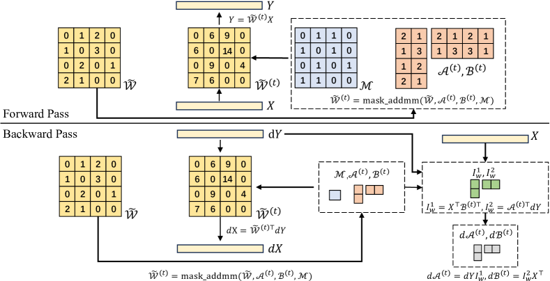
Finally, the workflow of LoRS is illustrated in Figure 1. Meanwhile, algorithm 1 and 2 details the forward pass and backward pass of LoRS. It can be seen that after optimization, LoRS only needs to store parameters in the computational graph, and at the same time, it only needs the MACs of in the forward pass and in the backward pass. Compared to LoRA, LoRS reduces the parameters stored in the computational graph and increases only the MACs of , superior to SP-LoRA, which increases the parameters stored in the computational graph and increases the MACs of .
2.4 Performance Optimization
The existing SP-LoRA methods SPP and SQFT use zero initialization and random initialization to initialize the adapters. However, recent advances in LoRA variants highlight the critical impact of initialization strategies on overall performance. Drawing inspiration from the methodologies of LoRA-GA Wang et al. (2024), we introduce a gradient-based initialization technique aimed at enhancing LoRS’s effectiveness.
Referring to existing LoRA variants, we initialize to 0, while minimizing the difference between LoRS and full fine-tuning on the first training iteration by initializing . To illustrate, with and disregarding masking operations, we derive the following equations:
This derivation illustrates the relation between the adapters and the gradient obtained from the initial training step. Therefore, we determine through an optimization process as follow:
| (4) |
This optimization objective can be solved by singular value decomposition, i.e., .
While the gradient-based initialization does require access to the gradients of the weight matrices during the first training step, we adopt layer-by-layer initialization strategy to ensure that this process can be carried out without imposing additional memory costs. This efficient initialization paves the way for improved performance in subsequent training iterations.
3 Experiments
| Model | Method | Sparsity | ARC-c | ARC-e | BoolQ | Hellaswag | OBQA | RTE | Winogrande | Average |
| Llama-2-7B | None | None | 43.52 | 76.35 | 77.74 | 57.14 | 31.40 | 62.82 | 69.06 | 59.72 |
| SparseGPT | 2:4 | 31.31 | 63.93 | 68.90 | 43.54 | 24.60 | 63.18 | 65.90 | 51.62 | |
| SparseGPT+SPP | 2:4 | 36.86 | 69.15 | 72.91 | 50.67 | 28.80 | 62.45 | 66.30 | 55.31 | |
| SparseGPT+SQFT | 2:4 | 36.01 | 64.35 | 72.17 | 51.84 | 29.60 | 59.93 | 63.61 | 53.93 | |
| SparseGPT+LoRS | 2:4 | 37.63 | 70.03 | 74.22 | 51.95 | 30.20 | 63.90 | 66.38 | 56.33 | |
| Wanda | 2:4 | 30.03 | 61.95 | 68.32 | 41.21 | 24.20 | 53.07 | 62.35 | 48.73 | |
| Wanda+SPP | 2:4 | 36.26 | 69.44 | 72.02 | 49.64 | 27.80 | 55.96 | 63.77 | 53.56 | |
| Wanda+SQFT | 2:4 | 35.41 | 65.03 | 72.39 | 50.18 | 30.00 | 60.29 | 62.67 | 53.71 | |
| Wanda+LoRS | 2:4 | 37.12 | 70.71 | 71.56 | 51.18 | 27.60 | 57.76 | 64.48 | 54.34 | |
| Llama-3-8B | None | 2:4 | 50.26 | 80.09 | 81.35 | 60.18 | 34.80 | 69.31 | 72.38 | 64.05 |
| SparseGPT | 2:4 | 32.00 | 62.67 | 73.70 | 43.19 | 22.20 | 53.79 | 65.75 | 50.47 | |
| SparseGPT+SPP | 2:4 | 40.78 | 71.09 | 75.35 | 52.01 | 26.40 | 59.93 | 67.88 | 56.21 | |
| SparseGPT+SQFT | 2:4 | 38.05 | 64.02 | 73.27 | 48.89 | 25.20 | 60.65 | 62.12 | 53.17 | |
| SparseGPT+LoRS | 2:4 | 40.70 | 70.96 | 79.08 | 53.26 | 28.00 | 60.65 | 67.17 | 57.94 | |
| Wanda | 2:4 | 26.45 | 55.93 | 66.18 | 37.51 | 18.60 | 52.71 | 60.06 | 45.35 | |
| Wanda+SPP | 2:4 | 38.48 | 68.64 | 74.77 | 49.53 | 25.20 | 58.48 | 64.64 | 54.25 | |
| Wanda+SQFT | 2:4 | 37.46 | 65.07 | 73.36 | 49.48 | 26.00 | 63.18 | 62.75 | 53.90 | |
| Wanda+LoRS | 2:4 | 40.78 | 70.37 | 77.03 | 51.54 | 26.00 | 67.87 | 64.80 | 56.91 |
| Model | Method | Sparsity | ARC-c | ARC-e | BoolQ | Hellaswag | OBQA | RTE | Winogrande | Average |
|---|---|---|---|---|---|---|---|---|---|---|
| Llama-2-13B | None | None | 48.38 | 79.42 | 80.55 | 60.04 | 35.20 | 65.34 | 72.30 | 63.03 |
| SparseGPT | 2:4 | 37.29 | 69.07 | 79.05 | 48.00 | 25.80 | 58.84 | 69.14 | 55.31 | |
| SparseGPT+SPP | 2:4 | 42.06 | 73.32 | 78.62 | 55.02 | 29.40 | 65.70 | 69.77 | 59.13 | |
| SparseGPT+SQFT | 2:4 | 40.78 | 67.93 | 76.48 | 54.68 | 29.40 | 71.12 | 69.38 | 58.54 | |
| SparseGPT+LoRS | 2:4 | 42.32 | 74.24 | 77.52 | 55.81 | 30.00 | 68.95 | 70.56 | 59.91 | |
| Wanda | 2:4 | 34.47 | 68.48 | 75.72 | 46.39 | 24.40 | 57.04 | 66.69 | 53.31 | |
| Wanda+SPP | 2:4 | 39.42 | 69.40 | 77.37 | 54.84 | 30.40 | 65.34 | 68.27 | 57.86 | |
| Wanda+SQFT | 2:4 | 40.02 | 68.35 | 76.09 | 54.17 | 29.80 | 64.98 | 66.93 | 57.19 | |
| Wanda+LoRS | 2:4 | 41.04 | 72.10 | 77.46 | 55.46 | 29.40 | 68.95 | 67.09 | 58.79 |
| Model | Method | Sparsity | ARC-c | ARC-e | BoolQ | Hellaswag | OBQA | RTE | Winogrande | Average |
|---|---|---|---|---|---|---|---|---|---|---|
| Llama-3-8B | SparseGPT | unstructured | 42.66 | 73.95 | 77.16 | 53.86 | 29.40 | 58.84 | 72.30 | 58.31 |
| SparseGPT+SPP | unstructured | 47.53 | 77.86 | 80.09 | 57.77 | 32.00 | 65.70 | 72.53 | 61.92 | |
| SparseGPT+SQFT | unstructured | 46.76 | 77.06 | 80.70 | 56.76 | 30.60 | 64.98 | 72.93 | 61.39 | |
| SparseGPT+LoRS | unstructured | 49.15 | 76.64 | 81.71 | 57.66 | 31.00 | 69.31 | 72.45 | 62.56 |
| Model | Method | Sparsity | ARC-c | ARC-e | BoolQ | Hellaswag | OBQA | RTE | Winogrande | Average |
|---|---|---|---|---|---|---|---|---|---|---|
| Llama-3-8B | SparseGPT | 2:4 | 32.00 | 62.67 | 73.70 | 43.19 | 22.20 | 53.79 | 65.75 | 50.47 |
| SparseGPT+SPP | 2:4 | 39.42 | 69.95 | 71.93 | 51.67 | 25.80 | 63.18 | 68.27 | 55.75 | |
| SparseGPT+SQFT | 2:4 | 38.14 | 70.29 | 75.87 | 52.35 | 26.80 | 63.90 | 67.56 | 56.42 | |
| SparseGPT+LoRS | 2:4 | 39.16 | 70.50 | 75.60 | 52.27 | 27.40 | 63.54 | 67.48 | 56.56 | |
| Wanda | 2:4 | 26.45 | 55.93 | 66.18 | 37.51 | 18.60 | 52.71 | 60.06 | 45.35 | |
| Wanda+SPP | 2:4 | 36.77 | 67.39 | 72.97 | 49.49 | 25.80 | 59.21 | 64.88 | 53.79 | |
| Wanda+SQFT | 2:4 | 38.31 | 69.53 | 71.56 | 50.83 | 28.00 | 54.87 | 66.30 | 54.20 | |
| Wanda+LoRS | 2:4 | 38.57 | 69.61 | 72.87 | 50.60 | 27.80 | 61.73 | 64.64 | 55.12 |
In this section, we aim to demonstrate the efficacy of LoRS in training sparse Large Language Models (LLMs) through a series of experiments.
Metrics. We assessed both the LoRA and SP-LoRA methods based on two primary metrics:
-
•
Efficiency: This includes the memory consumption and computational time required during the fine-tuning process.
-
•
Performance: We measured this by evaluating the model’s accuracy across various downstream tasks.
3.1 Experiment Setup
Our experimental framework utilized several models from the Llama series: Llama-2-7B, Llama-2-13B and Llama-3-8B (Touvron et al., 2023a, b; Dubey et al., 2024). To create sparse models, we applied post-training pruning techniques, specifically SparseGPT Frantar and Alistarh (2023) and Wanda Sun et al. (2024), using unstructured and 2:4 structured sparsity patterns, following existing works. For the efficiency analysis, we fine-tuned the pruned models with varying batch sizes and adapter ranks to observe their impact on resource utilization. Then, the performance evaluation involved fine-tuning the pruned models on two types of datasets: instruction data and pre-training data. During this phase, adapters were incorporated into all sparse weight matrices within the models.
-
•
Instruction Data: For instruction tuning, we employed the Stanford-Alpaca dataset (Taori et al., 2023). Here, the adapter rank was also set to 16, and the batch size was set to 32 samples, with the learning rate remaining at .
-
•
Pre-training Data: We used a subset of the SlimPajama dataset (Penedo et al., 2023), containing 0.5 billion tokens. The setup for this experiment included setting the adapter rank to 16, the batch size to 256,000 tokens, and the learning rate to .
Following fine-tuning, we evaluated the zero-shot performance of the models on seven benchmark datasets from the EleutherAI LM Evaluation Harness (Gao et al., 2024): ARC-Challenge, ARC-Easy (Clark et al., 2018), BoolQ (Clark et al., 2019), Hellaswag (Zellers et al., 2019), OpenBookQA (Mihaylov et al., 2018), RTE, and Winogrande (Sakaguchi et al., 2019). All experiments were conducted on Nvidia A800-80G GPUs and Nvidia A6000-48G GPUs.
Baselines. To evaluate the effectiveness of LoRS, we compare LoRS with the SP-LoRA methods SPP and SQFT, two existing methods designed to tuning sparse LLMs while preserving sparsity. Refer to Appendix B for a more detailed explanation.
3.2 Experiment Results
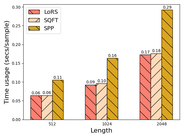
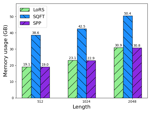
Efficiency Results. We evaluated the time and memory overhead of different methods via Llama-3-8B, including LoRS, SQFT and SPP. The implementation details for these methods are provided in Appendix A. We conducted experiments for sequence lengths from 512 to 2048 and for adapter ranks from 16 to 64, respectively. Figure 3 and 4 show the time usage and memory usage of the different methods for different sequence lengths, with the adapter rank being 16. It can be seen that LoRS outperforms SPP and SQFT in all scenarios in terms of training throughput and memory overhead, respectively. Compared to SPP, LoRS has a 40% increase in training speed while having the same memory footprint as SPP. LoRS, on the other hand, saves 40% of the memory footprint with the same training speed compared to SQFT. Figure 3, on the other hand, shows how the time overhead varies with the adapter rank size for a sequence length of 2048. It can be seen that changes in the adapter rank size have almost no impact on the time overhead. These results underscore the effectiveness of our approach, demonstrating that LoRS offers an optimal balance between performance and resource utilization when fine-tuning sparse LLMs.
Performance Results. Tables 1 and 2 present the zero-shot performance of the Llama-2-7B, Llama-3-8B and Llama-2-13B models, as well as their pruned and fine-tuned variants developed using the Stanford Alpaca under 2:4 sparsity type. Meanwhile, Table 3 shows the experimental results using unstructured sparsity types. The experimental findings reveal that LoRS significantly boosts the performance of sparse models, with improvements ranging from 7%~25% compared to models obtained through post-training pruning. In addition, the effectiveness of LoRS also exceeds that of existing SP-LoRA methods SPP and SQFT. Specifically, LoRS has a 1%~2% improvement over SPP and SQFT on the Alpaca dataset due to the better initialization used by LoRS. Table 4, on the other hand, present the results using the SlimPajama-0.5B datasets. On this dataset, LoRS has only minor enhancements compared to SPP and SQFT, this is due to it contains enough data that the impact of initialization on performance is reduced at this point.
4 Related Work
4.1 Pruning
Pruning is a technique for compressing neural networks by eliminating unimportant weights (Han et al., 2016). It can be divided into structured and unstructured pruning based on the sparsity pattern it induces. Structured pruning removes entire units like channels or layers to simplify the network’s architecture. In contrast, unstructured pruning targets individual weights, converting dense matrices into sparse ones. Advances in hardware have enabled efficient execution of models pruned with specific sparse patterns, such as 2:4 sparsity (Mishra et al., 2021). From an optimization standpoint, pruning methods are also classified as training-based or post-training. Training-based pruning gradually removes weights during the training phase by applying regularization techniques, which can introduce computational overhead and data requirements that are prohibitive for large models (Louizos et al., 2018; Sanh et al., 2020; Xia et al., 2022; Hu et al., 2024). Post-training pruning, however, allows for significant model compression using minimal calibration data, making it more suitable for large language models (Frantar and Alistarh, 2023; Sun et al., 2024; Zhang et al., 2024).
4.2 Parameter-Efficient Fine-Tuning (PEFT)
PEFT strategies enable fine-tuning of pre-trained models with minimal parameter updates. These methods typically freeze the original model and introduce trainable adapters, such as prefix tokens, side networks, or parallel/serial adapters (Liu et al., 2022; Zhang et al., 2020; Houlsby et al., 2019; Hu et al., 2023). LoRA and its variants are popular PEFT approaches that allow adapter parameters to merge with model weights after training (Hu et al., 2021; Zhang et al., 2023; Zhao et al., 2024). However, this merging process can negate the sparsity benefits in sparse LLMs. Our work focuses on adapting LoRA to maintain sparsity.
4.3 Sparsity-Preserved Training
Sparsity-preserved training methods aim to train sparse models from the outset or refine existing sparse models. Techniques like STE (Zhou et al., 2021b), RigL (Evci et al., 2021), and others (Huang et al., 2024; Kurtic et al., 2023) ensure that the trained models retain their sparse structure while achieving performance similar to dense counterparts. Despite their potential, these methods often require training all model parameters and can demand more GPU memory than training dense models, presenting challenges for LLM applications. Recent innovations, such as SPP Lu et al. (2024) and SQFT Munoz et al. (2024), attempt to mitigate this issue by integrating PEFT methods with sparsity-preserved training, offering a streamlined approach to training sparse models with reduced costs. Nonetheless, these methods still face high GPU memory overhead due to the construction of full-size matrices during forward passes.
5 Conclusion
In this paper, we present LoRS, a novel method designed to train sparse models in a parameter-efficient and memory-efficient manner while preserving sparsity. Our approach specifically tackles the challenges of domain adaptation and performance recovery for sparse large language models (LLMs). By building on the sparsity-preserving LoRA framework, LoRS achieves efficient fine-tuning of LLMs with reduced memory and computation usage through techniques including weight recompute and computational graph reording. Additionally, LoRS enhances the performance of fine-tuned models by employing more effective parameter initialization strategies.
Our experimental results on the Llama family demonstrate that LoRS can efficiently restore the performance of pruned LLMs, surpassing existing methods like SPP and SQFT. This highlights LoRS’s potential as an advanced solution for enhancing sparse models without compromising efficiency or performance.
References
- Bengio et al. (2013) Yoshua Bengio, Nicholas Léonard, and Aaron Courville. 2013. Estimating or propagating gradients through stochastic neurons for conditional computation. arXiv preprint arXiv:1308.3432.
- Chen et al. (2016) Tianqi Chen, Bing Xu, Chiyuan Zhang, and Carlos Guestrin. 2016. Training deep nets with sublinear memory cost. Preprint, arXiv:1604.06174.
- Clark et al. (2019) Christopher Clark, Kenton Lee, Ming-Wei Chang, Tom Kwiatkowski, Michael Collins, and Kristina Toutanova. 2019. Boolq: Exploring the surprising difficulty of natural yes/no questions. Preprint, arXiv:1905.10044.
- Clark et al. (2018) Peter Clark, Isaac Cowhey, Oren Etzioni, Tushar Khot, Ashish Sabharwal, Carissa Schoenick, and Oyvind Tafjord. 2018. Think you have solved question answering? try arc, the ai2 reasoning challenge. Preprint, arXiv:1803.05457.
- Dubey et al. (2024) Abhimanyu Dubey, Abhinav Jauhri, Abhinav Pandey, Abhishek Kadian, Ahmad Al-Dahle, Aiesha Letman, Akhil Mathur, Alan Schelten, Amy Yang, Angela Fan, Anirudh Goyal, and et al. 2024. The llama 3 herd of models. Preprint, arXiv:2407.21783.
- Evci et al. (2021) Utku Evci, Trevor Gale, Jacob Menick, Pablo Samuel Castro, and Erich Elsen. 2021. Rigging the lottery: Making all tickets winners. Preprint, arXiv:1911.11134.
- Frantar and Alistarh (2023) Elias Frantar and Dan Alistarh. 2023. Sparsegpt: Massive language models can be accurately pruned in one-shot. Preprint, arXiv:2301.00774.
- Gao et al. (2024) Leo Gao, Jonathan Tow, Baber Abbasi, Stella Biderman, Sid Black, Anthony DiPofi, Charles Foster, Laurence Golding, Jeffrey Hsu, Alain Le Noac’h, Haonan Li, Kyle McDonell, Niklas Muennighoff, Chris Ociepa, Jason Phang, Laria Reynolds, Hailey Schoelkopf, Aviya Skowron, Lintang Sutawika, Eric Tang, Anish Thite, Ben Wang, Kevin Wang, and Andy Zou. 2024. A framework for few-shot language model evaluation.
- Han et al. (2016) Song Han, Huizi Mao, and William J. Dally. 2016. Deep compression: Compressing deep neural networks with pruning, trained quantization and huffman coding. Preprint, arXiv:1510.00149.
- Houlsby et al. (2019) Neil Houlsby, Andrei Giurgiu, Stanislaw Jastrzebski, Bruna Morrone, Quentin de Laroussilhe, Andrea Gesmundo, Mona Attariyan, and Sylvain Gelly. 2019. Parameter-efficient transfer learning for nlp. Preprint, arXiv:1902.00751.
- Hu et al. (2021) Edward J. Hu, Yelong Shen, Phillip Wallis, Zeyuan Allen-Zhu, Yuanzhi Li, Shean Wang, Lu Wang, and Weizhu Chen. 2021. Lora: Low-rank adaptation of large language models. Preprint, arXiv:2106.09685.
- Hu et al. (2024) Yuxuan Hu, Jing Zhang, Zhe Zhao, Chen Zhao, Xiaodong Chen, Cuiping Li, and Hong Chen. 2024. : Enhancing structured pruning via pca projection. Preprint, arXiv:2308.16475.
- Hu et al. (2023) Zhiqiang Hu, Lei Wang, Yihuai Lan, Wanyu Xu, Ee-Peng Lim, Lidong Bing, Xing Xu, Soujanya Poria, and Roy Ka-Wei Lee. 2023. Llm-adapters: An adapter family for parameter-efficient fine-tuning of large language models. Preprint, arXiv:2304.01933.
- Huang et al. (2024) Weiyu Huang, Yuezhou Hu, Guohao Jian, Jun Zhu, and Jianfei Chen. 2024. Pruning large language models with semi-structural adaptive sparse training. Preprint, arXiv:2407.20584.
- Kurtic et al. (2023) Eldar Kurtic, Denis Kuznedelev, Elias Frantar, Michael Goin, and Dan Alistarh. 2023. Sparse fine-tuning for inference acceleration of large language models. Preprint, arXiv:2310.06927.
- Liu et al. (2022) Xiao Liu, Kaixuan Ji, Yicheng Fu, Weng Tam, Zhengxiao Du, Zhilin Yang, and Jie Tang. 2022. P-tuning: Prompt tuning can be comparable to fine-tuning across scales and tasks. In Proceedings of the 60th Annual Meeting of the Association for Computational Linguistics (Volume 2: Short Papers), pages 61–68, Dublin, Ireland. Association for Computational Linguistics.
- Louizos et al. (2018) Christos Louizos, Max Welling, and Diederik P. Kingma. 2018. Learning sparse neural networks through regularization. Preprint, arXiv:1712.01312.
- Lu et al. (2024) Xudong Lu, Aojun Zhou, Yuhui Xu, Renrui Zhang, Peng Gao, and Hongsheng Li. 2024. Spp: Sparsity-preserved parameter-efficient fine-tuning for large language models. Preprint, arXiv:2405.16057.
- Mihaylov et al. (2018) Todor Mihaylov, Peter Clark, Tushar Khot, and Ashish Sabharwal. 2018. Can a suit of armor conduct electricity? a new dataset for open book question answering. Preprint, arXiv:1809.02789.
- Mishra et al. (2021) Asit Mishra, Jorge Albericio Latorre, Jeff Pool, Darko Stosic, Dusan Stosic, Ganesh Venkatesh, Chong Yu, and Paulius Micikevicius. 2021. Accelerating sparse deep neural networks. Preprint, arXiv:2104.08378.
- Munoz et al. (2024) Juan Pablo Munoz, Jinjie Yuan, and Nilesh Jain. 2024. SQFT: Low-cost model adaptation in low-precision sparse foundation models. In Findings of the Association for Computational Linguistics: EMNLP 2024, pages 12817–12832, Miami, Florida, USA. Association for Computational Linguistics.
- Penedo et al. (2023) Guilherme Penedo, Quentin Malartic, Daniel Hesslow, Ruxandra Cojocaru, Alessandro Cappelli, Hamza Alobeidli, Baptiste Pannier, Ebtesam Almazrouei, and Julien Launay. 2023. The refinedweb dataset for falcon llm: outperforming curated corpora with web data, and web data only. arXiv preprint arXiv:2306.01116.
- Sakaguchi et al. (2019) Keisuke Sakaguchi, Ronan Le Bras, Chandra Bhagavatula, and Yejin Choi. 2019. Winogrande: An adversarial winograd schema challenge at scale. Preprint, arXiv:1907.10641.
- Sanh et al. (2020) Victor Sanh, Thomas Wolf, and Alexander M. Rush. 2020. Movement pruning: Adaptive sparsity by fine-tuning. Preprint, arXiv:2005.07683.
- Sun et al. (2024) Mingjie Sun, Zhuang Liu, Anna Bair, and J. Zico Kolter. 2024. A simple and effective pruning approach for large language models. Preprint, arXiv:2306.11695.
- Taori et al. (2023) Rohan Taori, Ishaan Gulrajani, Tianyi Zhang, Yann Dubois, Xuechen Li, Carlos Guestrin, Percy Liang, and Tatsunori B. Hashimoto. 2023. Stanford alpaca: An instruction-following llama model. https://github.com/tatsu-lab/stanford_alpaca.
- Touvron et al. (2023a) Hugo Touvron, Thibaut Lavril, Gautier Izacard, Xavier Martinet, Marie-Anne Lachaux, Timothée Lacroix, Baptiste Rozière, Naman Goyal, Eric Hambro, Faisal Azhar, Aurelien Rodriguez, Armand Joulin, Edouard Grave, and Guillaume Lample. 2023a. Llama: Open and efficient foundation language models. Preprint, arXiv:2302.13971.
- Touvron et al. (2023b) Hugo Touvron, Louis Martin, Kevin Stone, Peter Albert, Amjad Almahairi, Yasmine Babaei, Nikolay Bashlykov, Soumya Batra, Prajjwal Bhargava, Shruti Bhosale, Dan Bikel, and et al. 2023b. Llama 2: Open foundation and fine-tuned chat models. Preprint, arXiv:2307.09288.
- Wang et al. (2024) Shaowen Wang, Linxi Yu, and Jian Li. 2024. Lora-ga: Low-rank adaptation with gradient approximation. arXiv preprint arXiv:2407.05000.
- Xia et al. (2022) Mengzhou Xia, Zexuan Zhong, and Danqi Chen. 2022. Structured pruning learns compact and accurate models. arXiv preprint arXiv:2204.00408.
- Zellers et al. (2019) Rowan Zellers, Ari Holtzman, Yonatan Bisk, Ali Farhadi, and Yejin Choi. 2019. Hellaswag: Can a machine really finish your sentence? Preprint, arXiv:1905.07830.
- Zhang et al. (2020) Jeffrey O Zhang, Alexander Sax, Amir Zamir, Leonidas Guibas, and Jitendra Malik. 2020. Side-tuning: A baseline for network adaptation via additive side networks. Preprint, arXiv:1912.13503.
- Zhang et al. (2023) Longteng Zhang, Lin Zhang, Shaohuai Shi, Xiaowen Chu, and Bo Li. 2023. Lora-fa: Memory-efficient low-rank adaptation for large language models fine-tuning. Preprint, arXiv:2308.03303.
- Zhang et al. (2024) Yingtao Zhang, Haoli Bai, Haokun Lin, Jialin Zhao, Lu Hou, and Carlo Vittorio Cannistraci. 2024. Plug-and-play: An efficient post-training pruning method for large language models. In The Twelfth International Conference on Learning Representations.
- Zhao et al. (2024) Jiawei Zhao, Zhenyu Zhang, Beidi Chen, Zhangyang Wang, Anima Anandkumar, and Yuandong Tian. 2024. Galore: Memory-efficient llm training by gradient low-rank projection. Preprint, arXiv:2403.03507.
- Zhou et al. (2021a) Aojun Zhou, Yukun Ma, Junnan Zhu, Jianbo Liu, Zhijie Zhang, Kun Yuan, Wenxiu Sun, and Hongsheng Li. 2021a. Learning n:m fine-grained structured sparse neural networks from scratch. Preprint, arXiv:2102.04010.
- Zhou et al. (2021b) Aojun Zhou, Yukun Ma, Junnan Zhu, Jianbo Liu, Zhijie Zhang, Kun Yuan, Wenxiu Sun, and Hongsheng Li. 2021b. Learning n:m fine-grained structured sparse neural networks from scratch. Preprint, arXiv:2102.04010.
Appendix A Implementation of SPP, SQFT and LoRS
Appendix B SPP and SQFT
SPP (Lu et al., 2024) is a parameter-efficient and sparsity-preserving fine-tuning method. The formulation of SPP can be mathematically described as follows:
where denotes the sparse weight matrix, and represent the learnable parameter matrices, and means repeating the tensor along axis for times. The adjustment to the weight matrix, denoted by , is formulated as the Hadamard product of these three matrices, thereby maintaining the sparsity structure inherent in the matrices involved. Furthermore, the parameters and are the only ones subject to training, which significantly reduces the parameters compared to that of , thus exemplifying the parameter efficiency of this approach.
It is observed that SPP can be conceptualized as a variant of LoRA. To illustrate this perspective, consider partitioning each sequence of consecutive elements within into segments, such that:
where each segment is a vector of length . Subsequently, we define a block-diagonal matrix constructed from these segments:
With this definition, the update rule for the weight matrix can be rewritten as:
Therefore, SPP can be interpreted as a LoRA variant that employs a specialized matrix , augmented with the initial weight matrix as a weight term, to achieve its parameter-efficient and sparsity-preserving properties.
The distinctions between SPP and LoRA can be delineated as follows:
-
•
SPP employs a composite weight matrix formed by stitching together multiple diagonal matrices, whereas LoRA utilizes a standard matrix as its weight matrix.
-
•
SPP incorporates the initial weight matrix as an additional weight term on the basis of LoRA.
SQFT (Munoz et al., 2024) is another parameter-efficient and sparsity-preserving fine-tuning method. The formulation of SQFT can be mathematically described as follows:
where denotes the sparse weight matrix, and represent the learnable parameter matrices.