Exponential Asymptotics for Translational Modes in the Discrete Nonlinear Schrödinger Model

Abstract

In the present work, we revisit the topic of translational eigenmodes in discrete models. We focus on the prototypical example of the discrete nonlinear Schrödinger equation, although the methodology presented is quite general. We tackle the relevant discrete system based on exponential asymptotics and start by deducing the well-known (and fairly generic) feature of the existence of two types of fixed points, namely site-centered and inter-site-centered. Then, turning to the stability problem, we not only retrieve the exponential scaling (as $e^{-\pi^{2}/(2\varepsilon)}$, where $\varepsilon$ denotes the spacing between nodes) and its corresponding prefactor power-law (as $\varepsilon^{-5/2}$), both of which had been previously obtained, but we also obtain a highly accurate leading-order prefactor and, importantly, the next-order correction, for the first time, to the best of our knowledge. This methodology paves the way for such an analysis in a wide range of lattice nonlinear dynamical equation models.

I Introduction

It is well-known (and has by now been extensively studied) that lattice nonlinear dynamical equations of dispersive type arise in a wide range of applications. These emerge, among others, in the dynamics of the electric field of light in optical waveguides [24], as well as in the mean-field dynamics of atomic Bose-Einstein condensates (BECs) in deep optical lattices [25]. They are also relevant to nonlinear coupled lattices of electrical circuits governed by Kirchhoff’s laws applied to nonlinear elements (such as capacitors) [31], as well as to coherent structures arising in elastic media and mechanical metamaterials such as granular crystals and variants thereof [26, 33]. Further settings of considerable impact involve the arrays of superconducting Josephson junctions in condensed matter physics [6, 35], as well as the denaturation models of the DNA double strand [30, 29].

Admittedly, there exists a wide variety of associated models, with different ones among them being of interest/relevance to different applications. For instance, the quintessential —within nonlinear science— models of the Fermi-Pasta-Ulam-Tsingou type [14, 36] are particularly well suited to granular systems, while discrete Klein-Gordon (variants of sine-Gordon) lattices [21] are tailored to superconducting Josephson junctions. However, arguably, a central envelope model that emerges in a wide range of applications consists of the discrete nonlinear Schrödinger (DNLS) equation [20, 12]. For the latter, the most canonical framework consists of arrays of optical waveguides (where its relevance and extensive findings, including in experiments, have been summarized in various reviews [24, 1]), but it has also been of value to other fields such as BECs with optical lattice potential wells forming the effective lattice nodes [25, 3].

In all of these models bearing on-site potentials (discrete Klein-Gordon (DKG) and DNLS ones, for instance), there exist some principal features that clearly distinguish the discrete case from the continuum one. Arguably, the most notable one is the breaking of a fundamental continuum symmetry of the problem, the translational invariance thereof. The latter is well-known through Noether theory to be associated with the conservation of momentum [27]. This, in turn, has significant consequences as concerns the prototypical solitary waves of the models [8]. Indeed, typically it is found that such models, instead of a single discrete analogue to a continuum wave, they bear two such discrete analogues. One of them is referred to as site-centered and the other as bond-centered or inter-site-centered. Perhaps even more importantly, one of these states is found to be spectrally stable (typically in DKG and DNLS models it is the site-centered one) and one is spectrally unstable (typically, the inter-site-centered one). This is because the invariance of translation within the continuum is reflected in a zero eigenvalue (pair — as the system is Hamiltonian and eigenvalues come in pairs), which upon the perturbation of discreteness can either move along the imaginary axis, in the spectrally stable site-centered case, or along the real axis, in the spectrally unstable bond-centered alternative.

It was realized a considerable while ago [17] (see also references therein) that the relevant bifurcation of this translational eigenmode has to be exponentially small. A heuristic argument to that effect hinges on the Taylor expansion of the second difference (see also below), which to all algebraic orders in the relevant lattice spacing parameter can be approximated by a sum involving even derivatives, none of which breaks translational invariance. Hence, the bifurcation of the relevant eigenvalue from the origin of the spectral plane of eigenvalues needs to be exponentially small. Indeed, the work of [17] sought to approximate this eigenvalue that was also observed in numerous other works, including, e.g., in [16, 20] etc. However, the relevant work developed a perturbative argument from the integrable analogue of the equation —the so-called Ablowitz-Ladik model [2]. This had, however, a distinct drawback: while it seemed to capture the correct exponentially small term (and even the prefactor thereof as concerns its scaling power on the lattice spacing), it was argued therein that the prefactor could not be properly captured, nor could corrections to this leading order behavior be assessed.

In the present work we definitively address the relevant problem. Indeed, we utilize an exponential asymptotics technique based on [9, 28, 22] (partially reminiscent of what was done for continuum problems with periodic potentials in the work of [15]) that enables us to identify the two different possible stationary solitary waves of the lattice. We then bring the corresponding result to the spectral stability analysis problem and observe its implications on the (formerly zero translational) eigenvalue. Our technique allows us to indeed compute definitively the relevant prefactor and even lends itself to the calculation of the next order correction. By using the rather numerically stringent test of multiplying the eigenvalue by the relevant exponential (and leveraging an accurate computation of the relevant eigenvalue down to the limit of double precision), we are able to showcase the asymptotic agreement of our prediction with the numerical findings. What’s more, this methodology provides the reader with a tool that is expected to naturally generalize to other models carrying this generic —within lattice dynamical settings— feature.

Our presentation is structured as follows. In section II, we briefly provide the model’s mathematical setup and notation. In section III, we focus on the existence problem and its corresponding solitary wave solution. Section IV details our stability findings. Finally, in section V, we summarize our results and present some possibilities for future studies.

II Model Setup

The 1D discretized nonlinear Schrödinger (DNLS) equation is given by [20]

$${\rm i}\frac{dQ_{n}}{dt}+\Delta_{2}Q_{n}+|Q_{n}|^{2}Q_{n}=0,$$ (1)

where the discrete Laplacian associated with the spacing $\varepsilon$ reads:

$$\Delta_{2}Q_{n}=\frac{Q_{n-1}-2Q_{n}+Q_{n+1}}{\varepsilon^{2}}.$$ (2)

The continuous 1D nonlinear Schrödinger (NLS) equation, i.e., the continuum limit of the model as $\varepsilon\rightarrow 0$ assumes the form:

$${\rm i}q_{t}+q_{xx}+|q|^{2}q=0.$$ (3)

While we will not tackle them in the present work, it is relevant to point out that our considerations can be extended firstly to the setting of the 1D discretized nonlinear Schrödinger equation involving next-to-nearest neighbors:

$$\Delta_{2}Q_{n}=-\frac{1}{12}Q_{n-2}+\frac{4}{3}Q_{n-1}-\frac{5}{2}Q_{n}+\frac{4}{3}Q_{n+1}-\frac{1}{12}Q_{n+2}.$$ (4)

and secondly to the more general realm of next-nearest neighbor interactions (cooperating or potentially competing with the nearest neighbor ones) in the modeling form:

$$\mu(Q_{n+2}-2Q_{n}+Q_{n-2})+{\rm i}\frac{dQ_{n}}{dt}+\Delta_{2}Q_{n}+|Q_{n}|^{2}Q_{n}=0$$ (5)

which is inspired by setups in the form of zigzag waveguide arrays [11, 34].

III Series Solution

Let us use the well-known standing wave form $Q_{n}={\rm e}^{{\rm i}\omega t}q_{n}$ in (1) to obtain the stationary DNLS,

$$-\omega q_{n}+\frac{1}{\varepsilon^{2}}({q_{n+1}-2q_{n}+q_{n-1}})+|q_{n}|^{2}q_{n}=0.$$ (6)

We take a continuum limit by setting $z=\varepsilon n$ and letting $q_{n}\equiv q(z)$ to obtain

$$-\omega q(z)+\frac{1}{\varepsilon^{2}}\left(q(z+\varepsilon)-2q(z)+q(z-\varepsilon)\right)+|q(z)|^{2}q(z)=0.$$ (7)

Expanding this as a power series in $\varepsilon$ gives the infinite-order differential equation

$$-\omega q(z)+2\sum_{m=1}^{\infty}\frac{\varepsilon^{2m-2}}{(2m)!}\frac{d^{2j}q(z)}{dz^{2j}}+|q(z)|^{2}q(z)=0.$$ (8)

We expand $q(z)$ as an asymptotic power series in $\varepsilon$ such that

$$q(z)\sim\sum_{j=0}^{\infty}\varepsilon^{2j}q_{j}(z)\quad\mathrm{as}\quad\varepsilon\to 0.$$ (9)

The leading-order solution $q_{0}(z)$ satisfies the (ODE resulting from the standing wave ansatz within the) continuous nonlinear Schrödinger equation (3). We select the soliton solution, given by

$$q_{0}(z)=\sqrt{2\omega}\sech[\sqrt{\omega}(z-z_{0})].$$ (10)

Notice that here without loss of generality, and taking advantage of the phase/gauge invariance of the model [20, 8], we have selected the real solution to the relevant problem. For simplicity in the subsequent analysis, we define $\tilde{z}=z-z_{0}$, and write our equations in terms of this shifted variable. Substituting (9) into (8) and noting that $q_{0}$ is real and positive gives the recurrence relation

$$-\omega q_{j}+2\sum_{m=1}^{\infty}\frac{1}{(2m)!}\frac{d^{2m}q_{j-m+1}}{d\tilde{z}^{2m}}+2q_{0}^{2}|q_{j}|+q_{0}^{2}q_{j}=0.$$ (11)

It will be useful to identify certain asymptotic properties of $q_{0}$. The tail asymptotics of $q_{0}$ are given by

$$q_{0}(\tilde{z})\sim 2\sqrt{2\omega}e^{-\sqrt{\omega}\tilde{z}}\quad\mathrm{as}\quad\tilde{z}\to\infty.$$ (12)

The leading-order solution is singular at

$$\tilde{z}_{s}=\pm\frac{1}{\sqrt{\omega}}\left[\frac{\pi{\rm i}}{2}+k\pi{\rm i}\right],$$ (13)

where $k\in\mathbb{Z}$. We will denote specific choices of $k$ as $\tilde{z}_{s,k}$ where appropriate. Near these points, we find

$$q_{0}(\tilde{z})\sim-\frac{{\rm i}\sqrt{2}}{\tilde{z}-\tilde{z}_{s}}+\frac{{\rm i}\omega}{3}{\sqrt{2}}(\tilde{z}-\tilde{z}_{s})\quad\mathrm{as}\quad\tilde{z}\to\tilde{z}_{s}.$$ (14)

The dominant exponentially small oscillations will arise from the singularities $\tilde{z}_{s,0}$ and $\tilde{z}_{s,-1}$. By rearranging (11), we can see that each term $q_{j}$ is obtained by repeatedly differentiating previous terms in the series, and we therefore expect singularities in $q_{j}$ for $j>0$ to also be located at the points in (13). The singularities will become stronger as $j$ increases.

Continuing the calculated terms using the recurrence relation (11) gives

$$\frac{d^{2}q_{1}}{d\tilde{z}^{2}}+\frac{1}{12}\frac{d^{4}q_{0}}{d\tilde{z}^{4}}+(3q_{0}^{2}-\omega)q_{1}=0.$$ (15)

Solving this gives the particular solution

$$q_{1}=\frac{\omega^{3/2}(9-7\cosh(2\sqrt{\omega}\tilde{z})+\sqrt{\omega}\tilde{z}\sinh(2\sqrt{\omega}\tilde{z}))}{24\sqrt{2}\cosh^{3}(\sqrt{\omega}\tilde{z})}.$$ (16)

Near the singularities at $\tilde{z}=\tilde{z}_{s}$, this has the asymptotic behaviour

$$q_{1}(\tilde{z})\sim\frac{{\rm i}\sqrt{2}}{3(\tilde{z}-\tilde{z}_{s})^{3}}+\frac{\pi\sqrt{\omega}}{24\sqrt{2}(\tilde{z}-\tilde{z}_{s})^{2}}\quad\mathrm{as}\quad\tilde{z}\to\tilde{z}_{s}.$$ (17)

III.1 Late-Order Asymptotics

We now need to determine the asymptotic behaviour of $q_{j}(\tilde{z})$ as $j\to\infty$. In singularly perturbed equations such as (8), obtaining $q_{j}$ requires repeatedly differentiating earlier terms in the series. This repeated differentiation causes the singularity strength to increase at subsequent orders, and the series terms to diverge in a predictable factorial-over-power fashion [10]. Based on this observation, [9] proposed that the asymptotic behaviour of $q_{j}$ as $j\to\infty$ can be written a sum of factorial-over-power terms with the form

$$q_{j}(\tilde{z})\sim\frac{Q(\tilde{z})\Gamma(2j+\gamma)}{\chi(\tilde{z})^{2j+\gamma}},$$ (18)

where $\chi(z)=0$ at some $\tilde{z}=\tilde{z}_{s}$, and each singular point $\tilde{z}_{s}$ generates late-order terms in the asymptotic behaviour.

We will determine $Q(\tilde{z})$, $\chi(\tilde{z})$ and $\gamma$. By substituting this expression into (11), we obtain

$$-\frac{\omega Q\Gamma(2j+\gamma)}{\chi^{2j+\gamma}}+2\sum_{m=1}^{j-1}\Bigg{[}\frac{(\chi^{\prime})^{2m}}{(2m)!}\frac{Q\Gamma(2j+2+\gamma)}{\chi^{2j+2+\gamma}}-\frac{(\chi^{\prime})^{2m-1}}{(2m-1)!} \frac{Q^{\prime}\Gamma(2j+1+\gamma)}{\chi^{2j+1+\gamma}}$$

$$+\frac{(\chi^{\prime})^{2m-2}}{(2m-2)!}\frac{Q^{\prime\prime}\Gamma(2j+\gamma)}{\chi^{2j+\gamma}}\Bigg{]} +\frac{3q_{0}^{2}Q\Gamma(2j+\gamma)}{\chi^{2j+\gamma}}+\ldots=0,$$ (19)

where the terms that we have retained are all $\mathcal{O}(q_{j})$ as $j\to\infty$, and all omitted terms are smaller in this limit than those retained, and $q_{j}(\tilde{z})$ is taken to be real-valued. Note that we omitted any term proportional to $\chi^{\prime\prime}$, which would appear at order $\mathcal{O}(q_{n+1/2})$, because we will find at $\mathcal{O}(q_{j+1})$ that $\chi^{\prime}$ is constant, and therefore $\chi^{\prime\prime}=0$.

III.1.1 Calculating the singulant, $\chi$

Balancing terms of $\mathcal{O}(q_{j+1})$ in (19) as $j\to\infty$ gives

$$2Q\sum_{m=1}^{j-1}\frac{(\chi^{\prime})^{2m}}{(2m)!}=0.$$ (20)

We can determine the leading-order solution of this in the limit that $j\to\infty$ by extending the upper bound of the summation term to infinity. This gives $\cosh(\chi^{\prime})=1$, or

$$\chi=2\pi{\rm i}\ell\left(\tilde{z}-\tilde{z}_{s}\right),$$ (21)

where $\ell\in\mathbb{Z}$ and the final term corresponds to the positive choice of sign in (13) with $k=0$. We select $\ell=1$ as the solution of interest, as this corresponds to the largest exponentially small term associated with the singularity at $\tilde{z}_{s,0}$.

From this, we conclude that there is a Stokes line in the solution, along the curve satisfying

$$\mathrm{Im}(\chi)=0,\qquad\mathrm{Re}(\chi)>0.$$ (22)

This configuration is shown in Figure 1, with the Stokes line being represented as a solid blue line. Without loss of generality, we will select the contribution so that it is zero on the left-hand side of the Stokes line, and is switched on as the line is crossed from left ($\tilde{z}<0$) to right ($\tilde{z}>0$).

Figure 1: Stokes structure for the discrete solitary wave solution. We could pick the exponentially small term to be zero on either the left or the right-hand side of the Stokes line, shown as a solid blue line; this choice does not affect the final result. There are additional singularities further along the imaginary axis in both directions that produce additional Stokes lines on the line $\mathrm{Re}(\tilde{z})=0$, represented as dotted blue lines, but these Stokes lines switch on asymptotic contributions that are exponentially small compared to those considered here.

From (21), we see that $\chi^{*}$, or the complex conjugate of $\chi$ is a solution to this equation, and this corresponds to the largest exponentially small term associated with the singularity at $\tilde{z}_{s,-1}$. This will produce a second Stokes line along the curve $\mathrm{Re}(\tilde{z})=0$, across which another exponentially small contribution appears. This contribution will be the complex conjugate of the contribution associated with $\chi$ on the real axis, meaning that the total exponentially small contribution is real for $\tilde{z}\in\mathbb{R}$.

III.1.2 Calculating the prefactor, $Q$

At $\mathcal{O}(q_{j+1/2})$ as $j\to\infty$, we balance terms in (19) to obtain

$$2\sum_{m=1}^{j-1}\frac{Q^{\prime}(\chi^{\prime})^{2m-1}}{(2m-1)!}=0.$$ (23)

As $\chi^{\prime}=2\pi{\rm i}\ell$, this statement is always true when $j\to\infty$. This is a generic feature of such discrete systems, and appears in any discrete equation with only second-order differences.

Balancing terms at the next order, $\mathcal{O}(q_{j})$, gives

$$2\sum_{m=1}^{j-1}\frac{Q^{\prime\prime}(\chi^{\prime})^{2m-2}}{(2m-2)!}+(3q_{0}^{2}-\omega)Q =0.$$ (24)

Extending the summation term to infinity gives, after some algebraic manipulation,

$$Q^{\prime\prime}+(6\sech^{2}(\sqrt{\omega}\tilde{z})-1)\omega Q=0.$$ (25)

This can be solved to give the prefactor

$$Q(\tilde{z})=K_{1}Q_{1}(\tilde{z})+K_{2}Q_{2}(\tilde{z}),$$ (26)

where $K_{1}$ and $K_{2}$ are constants that have yet to be determined, and

$$Q_{1}(\tilde{z}) =\tfrac{1}{2}\tanh(\sqrt{\omega}\tilde{z})\sech(\sqrt{\omega}\tilde{z}),$$ (27)

$$Q_{2}(\tilde{z}) =\sech(\sqrt{\omega}\tilde{z})\,\left(6\sqrt{\omega}\tilde{z}\tanh(\sqrt{\omega}\tilde{z})+\cosh(2\sqrt{\omega}\tilde{z})-5\right).$$ (28)

The limiting behaviour as $\tilde{z}\to\infty$ of these solutions is

$$Q_{1}(\tilde{z})\sim e^{-\sqrt{\omega}\tilde{z}},\qquad Q_{2}(\tilde{z})\sim e^{\sqrt{\omega}\tilde{z}}.$$ (29)

The asymptotic behaviour of these solutions as $\tilde{z}\to\tilde{z}_{s}$ is,

$$Q_{1}(\tilde{z})\sim-\frac{\rm i}{2\omega(\tilde{z}-\tilde{z}_{s})^{2}},\qquad Q_{2}(z)\sim\frac{3\pi}{\omega(\tilde{z}-\tilde{z}_{s})^{2}}.$$ (30)

III.1.3 Calculating $\gamma$

We use (14) in (25) to obtain the local governing equation near $\tilde{z}=\tilde{z}_{s}$,

$$Q^{\prime\prime}\sim\frac{6Q}{(\tilde{z}-\tilde{z}_{s})^{2}},$$ (31)

which tells us that the asymptotic behaviour of the solution is

$$Q(\tilde{z})\sim\Lambda_{1}(\tilde{z}-\tilde{z}_{s})^{3}+\frac{\Lambda_{2}}{(\tilde{z}-\tilde{z}_{s})^{2}},$$ (32)

where $\Lambda_{1}$ and $\Lambda_{2}$ are arbitrary constants yet to be determined. The asymptotic behaviour of $q_{j}$ near the singularity is dominated as $j\to\infty$ by the term containing $\Lambda_{1}$. Setting $Q\sim\Lambda_{1}(z-z_{s})^{3}$ near the singular point gives the local behaviour

$$q_{j}\sim\frac{\Lambda_{1}(\tilde{z}-\tilde{z}_{s})^{3}\Gamma(2j+\gamma)}{[2\pi{\rm i}(\tilde{z}-\tilde{z}_{s})]^{2j+\gamma}}\quad\mathrm{as}\quad j\to\infty,\,\tilde{z}\to\tilde{z}_{s}.$$ (33)

In order to be consistent with the leading-order asymptotics for $q_{0}$ from (14), we require that the singularity have strength of 1 when $j=0$. This gives $\gamma=4$. An equivalent analysis for the term containing $\Lambda_{2}$ gives $\gamma=-1$. The large-$j$ asymptotic behaviour of $q_{j}$ is therefore dominated by the late-order expression in (33), in which the factorial term has larger argument.

The constants $\Lambda_{1}$ and $\Lambda_{2}$ may be used to determine the constants $K_{1}$ and $K_{2}$ in (26). We expand this expression for $Q$ in (30) about the point $\tilde{z}=\tilde{z}_{s}$ to obtain

$$Q(\tilde{z})\sim\frac{-\tfrac{\mathrm{i}}{2}K_{1}+3\pi K_{2}}{(\tilde{z}-\tilde{z}_{s})^{2}}+\frac{-\tfrac{\mathrm{i}}{2}K_{1}+3\pi K_{2}}{6}-\frac{7(-\tfrac{\rm i}{2}K_{1}+3\pi K_{2})}{120}(\tilde{z}-\tilde{z}_{s})^{2}+\frac{4{\rm i}}{5}K_{2}(\tilde{z}-\tilde{z}_{s})^{3}+\ldots$$ (34)

Comparing this expression with (32) gives $\Lambda_{1}={4{\rm i}}K_{2}/5$ and $\Lambda_{2}=-{\rm i}K_{1}/2+3\pi K_{2}$. We therefore know that the asymptotic behaviour of $q_{j}$, described in (18), as $j\to\infty$ is dominated by factorial-over-power terms with the form

$$q_{j}\sim\frac{5}{4{\rm i}}\frac{\Lambda_{1}U_{2}(z)\Gamma(2j+4)}{[2\pi{\rm i}(z-z_{s})^{2j+4}]}\quad\mathrm{as}\quad j\to\infty.$$ (35)

In subsequent analysis, we will omit the subscript on and $\Lambda_{1}$ and $U_{2}$.

III.1.4 Calculating $\Lambda$

To calculate $\Lambda$, we must match the asymptotics of the late-order terms (33) with an inner expansion near the singularity at $\tilde{z}=\tilde{z}_{s}$. From the expression (9) we see that the series fails to be asymptotic if $q_{j}(\tilde{z})=\mathcal{O}(\varepsilon^{-2})$ in the small $\varepsilon$ limit, as the terms are no longer well-ordered. We see from (33) that this corresponds to $\tilde{z}-\tilde{z}_{s}=\mathcal{O}(\varepsilon)$. Motivated by this scaling, we define a new inner coordinate $\eta$ and inner variable $\hat{q}(\eta)$ such that

$$\tilde{z}-\tilde{z}_{s}=\varepsilon\eta,\qquad\hat{q}(\eta)=\frac{q(\tilde{z})}{\varepsilon}.$$ (36)

The rescaled inner equation becomes

$$-\varepsilon^{2}\omega\hat{q}(\eta)+2\sum_{m=1}^{\infty}\frac{1}{(2m)!}\frac{d^{2m}\hat{q}(\eta)}{d\eta^{2m}}+|\hat{q}(\eta)|^{2}\hat{q}(\eta) =0,$$ (37)

Taking only the leading-order asymptotic behaviour of (37) gives the inner system

$$2\sum_{m=1}^{\infty}\frac{1}{(2m)!}\frac{d^{2m}\hat{q}(\eta)}{d\eta^{2m}}+|\hat{q}(\eta)|^{2}\hat{q}(\eta) =0.$$ (38)

The value of $\omega$ does not influence the calculations at this scaling. Note that the inner scaled variable $\eta$ has returned the original discrete scaling, and this system is equivalent to

$$2[q(\eta+1)-q(\eta)+q(\eta-1)]+|q(\eta)|^{2}q(\eta) =0.$$ (39)

This is the leading order reduction for the discrete equation (1) in the vicinity of singular points. This observation connects the outer scaling in terms of $z$ with the large-$n$ asymptotics of the original discrete problem in terms of $n$.

We apply the asymptotic series in the limit that $|\eta|\to\infty$,

$$\hat{q}(\eta)\sim\sum_{j=0}^{\infty}\frac{\hat{q}_{j}}{\eta^{2j+1}}\quad\mathrm{as}\quad|\eta|\to\infty$$ (40)

Based on the local behaviour of leading-order solution (14), we set $q_{0}=-{\rm i}\sqrt{2}$. We can then substitute (40) into (38) and balance powers of $\eta$ to obtain a recurrence relation for $q_{n}$, given by

$$2\sum_{j=1}^{n}\binom{2n+2}{2j}\hat{q}_{n-j+1}+\sum_{j=0}^{n}\sum_{k=0}^{n-j}\hat{q}_{j}\hat{q}_{k}\hat{q}_{n-j-k} =0.$$ (41)

These equations may be repeatedly solved for $\hat{q}_{n}$ up to arbitrary order. To determine the value of $\Lambda$, we match the value of $\hat{q}_{n}$ for large values of $n$ with the late-order term ansatz (33). By expressing the inner series (40) in terms of the outer variables, we find that matching $\hat{q}_{n}$ with the late-order ansatz requires that the asymptotic matching condition

$$\frac{\hat{q}_{n}}{(\tilde{z}-\tilde{z}_{s})^{2n+1}}\sim\frac{\Lambda(\tilde{z}-\tilde{z}_{s})^{3}\Gamma(2j+4)}{[2\pi\mathrm{i}(\tilde{z}-\tilde{z}_{s})]^{2j+4}}$$ (42)

be satisfied as $n\to\infty$. By rearranging this, we find that

$$\Lambda=\lim_{n\to\infty}\frac{(2\pi{\rm i})^{2n+4}\hat{q}_{n}}{\Gamma(2j+4)}.$$ (43)

To approximate this value, we calculate $\hat{q}_{n}$ numerically for large values of $n$. These values are then substituted into the expression from (43) to obtain an approximate value for $\Lambda$, denoted $\Lambda_{\mathrm{app}}$. Figure 2 shows evidence that $\Lambda_{\mathrm{app}}$ converges as $n\to\infty$. Calculating up to $n=500$ gives $\Lambda\approx-358.513{\rm i}$.

Figure 2: First 100 approximate values of $\Lambda$.

III.2 Stokes Phenomenon

This procedure is essentially identical to King & Chapman [22]; however, that is a nonstandard application of the ideas from Olde Daalhuis et al [28], and we therefore outline the details in Appendix A. The general procedure is to truncate the asymptotic series (9) so that the truncation remainder is exponentially small, giving

$$q(\tilde{z})=\sum_{j=0}^{N-1}\varepsilon^{2n}q_{n}(\tilde{z})+q_{\mathrm{exp}},$$ (44)

where $N$ is the truncation value that minimizes the series approximation error, and $q_{\mathrm{exp}}$ is the remainder after truncation, which is exponentially small if $N$ is chosen optimally [5, 4]; in this case, we find that the correct value is $N=|\chi|/2\varepsilon+\alpha$, where $\alpha\in[0,1)$ is chosen so that $N$ is an integer. We substitute the truncated series (44) into the governing equation (8) to obtain an equation for $q_{\mathrm{exp}}$, given in (93), that we write in terms of the late-order ansatz (18) to obtain an equation (96) which we can study using asymptotic methods as $\varepsilon\to 0$.

We apply matched asymptotic expansions to study $q_{\mathrm{exp}}$ in a neighborhood of width $\mathcal{O}(\sqrt{\varepsilon})$ near the Stokes line in order to determine the exponentially small change in the asymptotic contribution that occurs within this neighborhood as the Stokes line is crossed from left to right. We are free to set $q_{\mathrm{exp}}$ to be zero on the left-hand side of the Stokes line, meaning that the change (107) gives the value of the exponentially small contribution on the right-hand side.

In this analysis we find that for $\tilde{z}>0$ the exponentially small contribution to the asymptotic behaviour, denoted $q_{\mathrm{exp}}$, satisfies

$$q_{\mathrm{exp}}\sim-\frac{2\pi{\rm i}}{\varepsilon^{4}}Qe^{-\chi/(\varepsilon\sqrt{\omega})}+\mathrm{c.c.}\quad\mathrm{as}\quad\varepsilon\to 0,$$ (45)

where we have included the complex conjugate quantity that switches on due to the singularity at $z_{s,-1}$. Simplifying this expression using (21) and (13) gives the exponentially small contribution for $\tilde{z}>0$ as

$$q_{\mathrm{exp}}\sim\frac{2\pi}{\varepsilon^{4}}Qe^{-\pi^{2}/(\varepsilon\sqrt{\omega})}\sin\left(\frac{2\pi\tilde{z}}{\varepsilon}\right)\quad\mathrm{as}\quad\varepsilon\to 0.$$ (46)

There is no exponentially small contribution present in the solution for $\tilde{z}<0$.

III.3 Site selection

The oscillations in (46) are exponentially small when they switch in amplitude across the Stokes line; however, as $z\to\infty$, the exponentially small oscillations in (46) grow as a consequence of to the exponentially growing behaviour of $Q$ described in (29). As $\tilde{z}\to\infty$ and $\varepsilon\to 0$, the remainder satisfies the expression

$$q_{\mathrm{exp}}\sim\frac{2\pi}{\varepsilon^{4}}\left(\frac{5\Lambda}{4{\rm i}}e^{\sqrt{\omega}\tilde{z}}\right)e^{-\pi^{2}/(\varepsilon\sqrt{\omega})}\sin\left(\frac{2\pi\tilde{z}}{\varepsilon}\right).$$ (47)

We can write this in the original discrete scaling using $\tilde{z}=\varepsilon(n-n_{0})$, and using the fact that $\Lambda$ is a negative imaginary number, to obtain

$$q_{\mathrm{exp}}\sim-\frac{5\pi|\Lambda|}{2\varepsilon^{4}}e^{\varepsilon\sqrt{\omega}(n-n_{0})}e^{-\pi^{2}/(\varepsilon\sqrt{\omega})}\sin\left(2\pi(n-n_{0})\right)\quad\mathrm{as}\quad n\to\infty,\,\varepsilon\to 0.$$ (48)

The presence of a slowly growing oscillatory tail in the asymptotic solution indicates that this solution can only exist if $n_{0}$ is chosen in a way such as to eliminate the oscillations entirely for integer values of $n$. There are only two values in $n_{0}\in[0,1)$ that achieve this; $n_{0}=0$, or on-site pinning, and $n_{0}=1/2$, or inter-site pinning. In this way we retrieve the well-known result about the existence of solely site-centered and inter-site-centered stationary solutions in the discrete lattice setting [12, 16, 20].

IV Stability

In the previous section we determined that as $\varepsilon\to 0$, if $z>z_{0}$ then

$$q(\tilde{z})\sim\sum_{j=0}^{N-1}\varepsilon^{2j}q_{j}(\tilde{z})+\frac{2\pi}{\varepsilon^{4}}Qe^{-\pi^{2}/(\varepsilon\sqrt{\omega})}\sin\left(\frac{2\pi\tilde{z}}{\varepsilon}\right).$$ (49)

We will subsequently refer to this steady solution as $q_{s}(\tilde{z})$. As $\tilde{z}\to\infty$, this asymptotic behavior is

$$q_{s}(z)\sim 2\sqrt{2\omega}e^{-\sqrt{\omega}\tilde{z}}+\sum_{j=1}^{N-1}\varepsilon^{2j}q_{j}(z)-\frac{2\pi}{\varepsilon^{4}}\left(\frac{5{\rm i}\Lambda}{4}\mathrm{e}^{\sqrt{\omega}\tilde{z}}\right)e^{-\pi^{2}/(\varepsilon\sqrt{\omega})}\sin\left(\frac{2\pi\tilde{z}}{\varepsilon}\right),$$ (50)

as ${\tilde{z}}\to\infty$, $\varepsilon\to 0$. We assume that $n_{0}$, and hence $z_{0}$, is chosen so that we have either an site-centered or inter-site-centered solution. We introduce perturbations of the form

$$Q=e^{{\rm i}\omega t}\left[q_{s}+fe^{\lambda t}+g^{*}e^{\lambda^{*}t}\right].$$ (51)

By direct substitution, we obtain

$$2\sum_{m=1}^{\infty}\frac{\varepsilon^{2m-2}}{(2m)!}\frac{d^{2m}f}{d\tilde{z}^{2m}}+q_{s}^{2}(2f+g)-\omega f =-{\rm i}\lambda f,$$ (52)

$$2\sum_{m=1}^{\infty}\frac{\varepsilon^{2m-2}}{(2m)!}\frac{d^{2m}g}{d\tilde{z}^{2m}}+q_{s}^{2}(2g+f)-\omega g ={\rm i}\lambda g.$$ (53)

We make the transformation $v=f+g$, $w=f-g$, giving

$$\mathcal{L}_{0}v=-{\rm i}\lambda w,\qquad\mathcal{L}_{1}w={\rm i}\lambda v,$$ (54)

where

$$\mathcal{L}_{0}=2\sum_{m=1}^{\infty}\frac{\varepsilon^{2m-2}}{(2m)!}\frac{d^{2m}}{d{\tilde{z}}^{2m}}+3q_{s}^{2}-\omega,\qquad\mathcal{L}_{1}=2\sum_{m=1}^{\infty}\frac{\varepsilon^{2m-2}}{(2m)!}\frac{d^{2m}}{d{\tilde{z}}^{2m}}+q_{s}^{2}-\omega.$$ (55)

We expand $v$ and $w$ as power series in the eigenvalue $\lambda$ in the limit $\lambda\to 0$, giving the leading-order equations

$$\mathcal{L}_{0}v_{0}=0,\qquad\mathcal{L}_{1}w_{0} =0.$$ (56)

We consider two eigenfunctions; one associated with translation and one associated with phase invariance. We can study these by setting (as is well-known [19, 8])

$$v_{0}=\frac{dq_{s}}{{d\tilde{z}}},\qquad w_{0}=0,$$ (57)

for the eigenvector associated with translation invariance, and

$$v_{0}=0,\qquad w_{0}={\rm i}q_{s},$$ (58)

for the one associated with phase invariance. These choices solve (56).

IV.1 First eigenvalue

IV.1.1 Leading order

To calculate the eigenvalue associated with translation invariance, we apply (57) to obtain $w_{0}=0$ and

$$v_{0}\sim-\frac{5|\Lambda|\pi^{2}}{\varepsilon^{5}}e^{\sqrt{\omega}\tilde{z}}\mathrm{e}^{-\pi^{2}/(\varepsilon\sqrt{\omega})}\cos\left(\frac{2\pi\tilde{z}}{\varepsilon}\right)\quad\mathrm{as}\quad\tilde{z}\to\infty,\,\varepsilon\to 0.$$ (59)

We now balance terms in (54) at $\mathcal{O}(\lambda)$ to obtain

$$\mathcal{L}_{0}v_{1}=0,\qquad\mathcal{L}_{1}w_{1}=-{\rm i}\frac{dq_{s}}{d\tilde{z}}.$$ (60)

The first equation gives $v_{1}=0$. Using $q_{s}\sim q_{0}$ as $\varepsilon\to 0$, we find

$$\frac{d^{2}w_{1}}{dz^{2}}+2\omega\sech^{2}(\sqrt{\omega}\tilde{z})w_{1}-\omega w_{1}\sim-{\rm i}\sqrt{2\omega}\sech(\sqrt{\omega}\tilde{z})\tanh(\sqrt{\omega}\tilde{z}).$$ (61)

The homogeneous solutions $W_{1}$ and $W_{2}$ are

$$W_{1}(z)=\sech(\sqrt{\omega}\tilde{z}),\qquad W_{2}(z)=\sqrt{\omega}\tilde{z}\sech(\sqrt{\omega}\tilde{z})+\sinh(\sqrt{\omega}\tilde{z}).$$ (62)

The general solution is

$$w_{1}=-\frac{{\rm i}\sqrt{2}}{2}W_{1}(\tilde{z})\int_{a}^{\tilde{z}} W_{2}(s)\sech(\sqrt{\omega}s)\tanh(\sqrt{\omega}s)ds$$

$$+\frac{{\rm i}\sqrt{2}}{2}W_{2}(\tilde{z})\int_{b}^{\tilde{z}}W_{1}(s)\sech(\sqrt{\omega}s)\tanh(\sqrt{\omega}s)ds.$$ (63)

where we are free to choose $a$ and $b$. These integrals can be evaluated exactly using (62). The function $W_{2}(z)\to\infty$ as $z\to\pm\infty$. We therefore select $b$ so that the second integral vanishes in this limit, or $b=-\infty$. The resulting expression is

$$w_{1}=-\frac{{\rm i}\sqrt{2\omega}}{2}\big{(}\tilde{z}\sech(\sqrt{\omega}\tilde{z})+\alpha W_{1}(\tilde{z})\big{)},$$ (64)

where $\alpha$ is a constant determined by the choice of $a$ in (63). As $W_{1}(z)$ decays in both directions, we do not obtain a condition on the choice of $\alpha$. The resulting expression for $w_{1}(\tilde{z})$ decays as $\tilde{z}\to\pm\infty$.

Balancing terms in (54) at $\mathcal{O}(\lambda^{2})$ gives

$$\mathcal{L}_{0}v_{2}=-{\rm i}w_{1},\qquad\mathcal{L}_{1}w_{2}=0.$$ (65)

We see that $w_{2}=0$, and $v_{2}$ satisfies

$$\frac{d^{2}v_{2}}{d\tilde{z}^{2}}+(3u_{s}^{2}-\omega)v_{2}=-\frac{\sqrt{2\omega}}{2}(\tilde{z}+\alpha)\sech(\sqrt{\omega}\tilde{z}).$$ (66)

The homogeneous solutions to this equation were given previously in (27)–(28). For consistency in notation within this section, we define

$$V_{1}(\tilde{z}) =\tfrac{1}{2}\tanh(\sqrt{\omega}\tilde{z})\sech(\sqrt{\omega}\tilde{z}),$$ (67)

$$V_{2}(\tilde{z}) =\sech(\sqrt{\omega}\tilde{z})\,\left(6\sqrt{\omega}\tilde{z}\tanh(\sqrt{\omega}\tilde{z})+\cosh(2\sqrt{\omega}\tilde{z})-5\right).$$ (68)

The general solution is

$$v_{2}=\frac{1}{2\sqrt{2}}V_{1}(\tilde{z})\int_{a}^{\tilde{z}} V_{2}(s)(s+\alpha)\sech(\sqrt{\omega}s)ds$$

$$-\frac{1}{2\sqrt{2}}V_{2}({\tilde{z}})\int_{b}^{\tilde{z}}V_{1}(s)(s+\alpha)\sech(\sqrt{\omega}s)ds,$$ (69)

where we are free to choose $a$ and $b$. The first term decays as $V_{1}({\tilde{z}})$, so we do not obtain any conditions on $a$. The second term grows as ${\tilde{z}}\to\pm\infty$. We can select $b$ to suppress growth on one side, but not both. We choose $b=-\infty$, which ensures that the second integral vanishes as ${\tilde{z}}\to-\infty$. As ${\tilde{z}}\to\infty$, we have

$$v_{2}\sim-\frac{1}{2\sqrt{2}}V_{2}({\tilde{z}})\int_{-\infty}^{\tilde{z}}V_{1}(s)(s+\alpha)\sech(\sqrt{\omega}s)ds=-\frac{V_{2}({\tilde{z}})}{4\sqrt{2}}\sim-\frac{e^{{\sqrt{\omega}\tilde{z}}}}{4\sqrt{2}}.$$ (70)

We are now able to predict the behaviour of the tail as $\tilde{z}\to\infty$. On lattice points, we have

$$v\sim v_{0}+\lambda^{2}v_{2}\sim-\frac{5|\Lambda|\pi^{2}}{\varepsilon^{5}}e^{\sqrt{\omega}\tilde{z}}e^{-\pi^{2}/(\varepsilon\sqrt{\omega})}\cos\left(\frac{2\pi\tilde{z}}{\varepsilon}\right)-\frac{\lambda^{2}e^{\sqrt{\omega}\tilde{z}}}{4\sqrt{2}}\quad\mathrm{as}\quad\tilde{z}\to\infty,\,\varepsilon\to 0.$$ (71)

Both terms grow large in the limit $z\to\infty$, and can only be avoided if the terms cancel precisely. This gives the condition that

$$v_{0}\sim-\lambda^{2}v_{2}\quad\mathrm{as}\quad\varepsilon\to 0.$$ (72)

Solving this expression for $\lambda$ and writing the result in terms of the original discrete variable $n$ gives

$$\lambda^{2}\sim-\frac{40\sqrt{2}|\Lambda|\pi^{2}}{\varepsilon^{5}}e^{-\pi^{2}/(\varepsilon\sqrt{\omega})}\cos\left({2\pi(n-n_{0})}\right)\quad\mathrm{as}\quad\varepsilon\to 0.$$ (73)

For on-site pinning $n_{0}$ is an integer, so $\lambda^{2}<0$. The eigenvalues are imaginary, and the on-site standing wave is stable. For inter-site pinning $n_{0}$ is a half-integer, so there is a positive real value for $\lambda$ and the corresponding waveform is unstable. In both cases, the eigenvalue has magnitude as $\varepsilon\to 0$

$$|\lambda|\sim\frac{2^{7/4}5^{1/2}\pi|\Lambda|^{1/2}e^{-\pi^{2}/(2\varepsilon\sqrt{\omega})}}{\varepsilon^{5/2}}\approx\frac{316.355e^{-\pi^{2}/(2\varepsilon\sqrt{\omega})}}{\varepsilon^{5/2}}.$$ (74)

To validate this prediction numerically, we will require the first correction term to $\lambda$ in the limit $\varepsilon\to 0$. It is also worthwhile to note that this prediction shares both the exponential dependence and the prefactor $\varepsilon$-scaling of the work of [17], yet has a different numerical prefactor than the $116.2$ of the latter work.

IV.1.2 First correction term

To determine the correction to the eigenvalue, we must match the asymptotic solution for $q$ with two terms of an inner expansion in the neighborhood of the singularity at $\tilde{z}=\tilde{z}_{s}$. To do this, we apply the trick introduced in [22] and find the first correction to the pole locations in $q(\tilde{z})$.

Combining the local expansions from (14) and (17) near $\tilde{z}=\tilde{z}_{s}$ gives

$$q\sim-\frac{{\rm i}\sqrt{2}}{\tilde{z}-\tilde{z}_{s}}+\frac{{\rm i}\omega}{3}{\sqrt{2}}(\tilde{z}-\tilde{z}_{s})+\varepsilon^{2}\left(\frac{{\rm i}\sqrt{2}}{3(\tilde{z}-\tilde{z}_{s})^{3}}+\frac{\pi\sqrt{\omega}}{24\sqrt{2}(\tilde{z}-\tilde{z}_{s})^{2}}\right)\quad\mathrm{as}\quad\varepsilon\to 0,\,\tilde{z}\to\tilde{z}_{s}.$$ (75)

Expressing this in terms of the inner variables $\varepsilon\eta=\tilde{z}-\tilde{z}_{s}$ and $\hat{q}(\eta)=\varepsilon q(\tilde{z})$, we find that

$$\hat{q}(\eta)\sim\left(-\frac{{\rm i}\sqrt{2}}{\eta}+\frac{{\rm i}\sqrt{2}}{3\eta^{2}}\right)+\frac{\varepsilon\pi\sqrt{\omega}}{24\sqrt{2}\eta}+\mathcal{O}(\varepsilon^{2})$$ (76)

as $\varepsilon\to 0$. We instead define the alternative inner variable $\varepsilon\hat{\eta}=\tilde{z}-\tilde{z}_{s}-\pi{\rm i}\sqrt{\omega}\varepsilon^{2}/48$.This inner variable is chosen to precisely cancel the $\mathcal{O}(\varepsilon)$ correction term, leaving

$$\hat{q}(\eta)\sim\left(-\frac{{\rm i}\sqrt{2}}{\hat{\eta}}+\frac{{\rm i}\sqrt{2}}{3\hat{\eta}^{2}}\right)+\mathcal{O}(\varepsilon^{2})$$ (77)

as $\varepsilon\to 0$, which is accurate to the required two terms. This tells us that the true pole location has an $\mathcal{O}(\varepsilon^{2})$ correction, and we set $\tilde{z}_{s,0}={\rm i}\pi/2\sqrt{\omega}+{\rm i}\pi\sqrt{\omega}\varepsilon^{2}/48$. This adjusts the value of $\chi=2\pi{\rm i}(\tilde{z}-\tilde{z}_{s})$ in (108), which in turn produces the adjusted exponentially-small remainder as $\varepsilon\to 0$ and $\tilde{z}\to\infty$

$$R \sim-\frac{5\pi|\Lambda|}{2\varepsilon^{4}}e^{\sqrt{\omega}\tilde{z}}e^{-\pi^{2}/(\varepsilon\sqrt{\omega})}e^{-\varepsilon\pi^{2}\sqrt{\omega}/48}\sin\left(\frac{2\pi\tilde{z}}{\varepsilon}\right)$$ (78)

$$\sim-\frac{5\pi|\Lambda|}{2\varepsilon^{4}}e^{\sqrt{\omega}\tilde{z}}e^{-\pi^{2}/(\varepsilon\sqrt{\omega})}\left(1-\frac{\varepsilon\pi^{2}\sqrt{\omega}}{24}\right)\sin\left(\frac{2\pi\tilde{z}}{\varepsilon}\right)$$ (79)

This allows us to determine the first correction in $\varepsilon$ to the eigenvalue $\lambda$. We find that

$$|\lambda| \sim\frac{2^{7/4}5^{1/2}\pi|\Lambda|^{1/2}e^{-\pi^{2}/(2\varepsilon\sqrt{\omega})}}{\varepsilon^{5/2}}\left(1-\frac{\varepsilon\pi^{2}\sqrt{\omega}}{24}\right)^{1/2}$$ (80)

$$\sim\frac{2^{7/4}5^{1/2}\pi|\Lambda|^{1/2}e^{-\pi^{2}/(2\varepsilon\sqrt{\omega})}}{\varepsilon^{5/2}}\left(1-\frac{\varepsilon\pi^{2}\sqrt{\omega}}{48}\right)\quad\mathrm{as}\quad\varepsilon\to 0.$$ (81)

Evaluating this expression gives the numerical approximation

$$|\lambda|\approx 316.355\left(1-\frac{\varepsilon\pi^{2}\sqrt{\omega}}{48}\right)\frac{\mathrm{e}^{-\pi^{2}/(2\varepsilon\sqrt{\omega})}}{\varepsilon^{5/2}}.$$ (82)

IV.1.3 Numerics

In order to examine the validity of the original prediction of Eq. (74) and the associated first correction term of Eq. (82), we have performed computations of the relevant eigenvalues for the case of the site-centered solitary waves and their associated stability. Such computations are admittedly not new, as they have earlier appeared in [16, 17, 20], however the distinguishing feature here is that we push further towards the relevant limit than was previously considered and, in addition, we plot them in a way that clearly brings forth the agreement with our theoretical predictions. Indeed, looking already at the right panel of Fig. 3, the agreement between the original prediction of Eq. (74) (black dash-dotted line) and the full numerical results seems very good. This agreement seems to be even further improved by the presence of the first correction term (red dashed line). It is important to appreciate here that the variation of the relevant eigenvalue occurs over more than 6 orders of magnitude for the interval of spacings $\varepsilon$ shown.

However, the true accuracy of our findings is much more clearly underscored by the far more demanding test of multiplying the eigenvalue findings by $\varepsilon^{5/2}\mathrm{e}^{\pi^{2}/(2\varepsilon\sqrt{\omega})}$. This rescaling not only strips the theoretical prediction of its dominant functional dependence, clearly distinguishing between the original form of Eq. (74) (which is now just a constant) and of Eq. (82) (which is now just a straight line). It also imposes a multiplication by a growing exponential which would be extremely sensitive towards a potential error in the relevant exponent. This clearly confirms not only the accuracy of the exponential dependence and of the power law prefactor; it also showcases the systematic approach to our asymptotic prediction in a quite definitive manner. It is relevant to note here that we have use a diverse palette of tools for obtaining these eigenvalues accurately to about $10^{-7}$. Seeking a further probing of the asymptotics requires tools that are considerably more refined at the level of the eigenvalue solver which, while not impossible, is outside the scope of the present work.

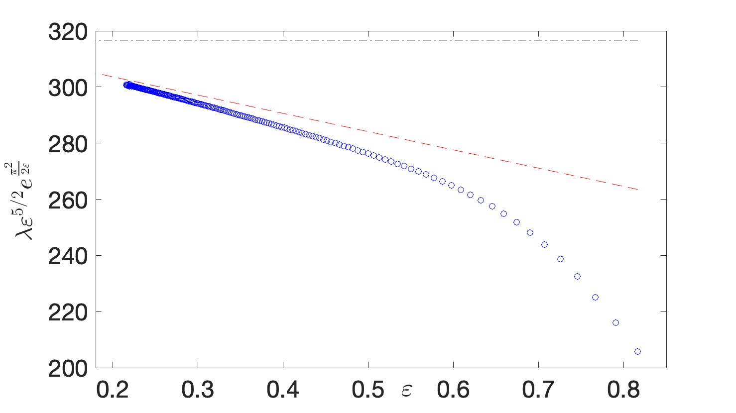
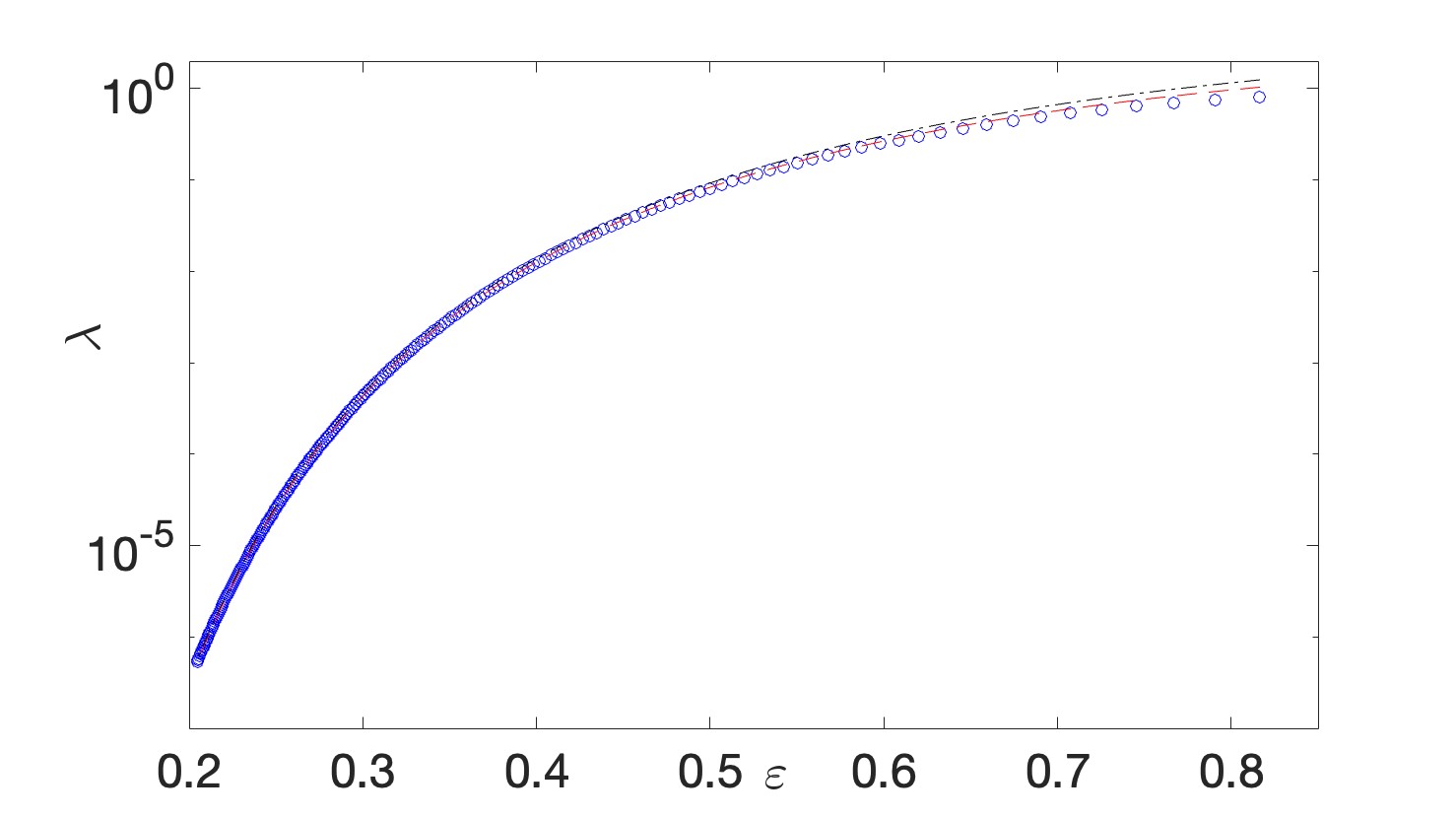
Figure 3: In the left panel we show the asymptotic predictions of our analysis herein, namely Eq. (74) by a black dash-dotted line, and its leading order correction of Eq. (82) by a red dashed line. These eigenvalue predictions (as a function of the lattice spacing $\varepsilon$) have been multiplied by $\varepsilon^{5/2}\mathrm{e}^{\pi^{2}/(2\varepsilon\sqrt{\omega})}$, so that the former one amounts to a constant and the latter to a straight line. These are compared to the correspondingly plotted eigenvalues associated with the site-centered solitary wave, plotted by blue circles. To illustrate how stringent of a test the left panel represents and showcase how close these 3 curves are as concerns the original eigenvalue itself, we can observe the same predictions/findings for $\lambda$ as a function of the coupling $\varepsilon$ in the right panel.

IV.2 Second eigenvalue

We may repeat the previous procedure in order to determine the second eigenvalue, using the perturbation

$$v_{0}=0,\qquad w_{0}={\rm i}u_{s}.$$ (83)

Following the analysis from before, $w_{1}=0$ and the equation for $v_{1}$ at leading order as $\lambda,\varepsilon\to 0$ is

$$\frac{d^{2}v_{1}}{d\tilde{z}^{2}}+(3u_{s}^{2}-\omega)v_{1}=u_{0}.$$ (84)

The homogeneous solutions are identical to (67)–(68). The general solution is given by

$$w_{2}=-\frac{V_{1}(\tilde{z})}{\sqrt{2}}\int_{a}^{\tilde{z}}V_{2}(s)\sech(s)\,ds+\frac{V_{2}(\tilde{z})}{\sqrt{2}}\int_{b}^{\tilde{z}}V_{1}(s)\sech(s)\,ds.$$ (85)

We select $b=-\infty$ to suppress growth $V_{2}$ as $\tilde{z}\to-\infty$, giving

$$v_{1}=\frac{\sech(\sqrt{\omega}{\tilde{z}})}{\sqrt{2\omega}}\left(1-\sqrt{\omega}(\tilde{z}+\alpha)\tanh(\sqrt{\omega}\tilde{z})\right),$$ (86)

where $\alpha$ is a constant that depends on the choice of $a$. Balancing terms at $\mathcal{O}(\lambda^{2})$, we find $v_{2}=0$ and

$$\frac{d^{2}w_{2}}{dz^{2}}+(u_{s}^{2}-\omega)w_{2}=-v_{1}.$$ (87)

The homogeneous solutions are given in (62). The general solution is

$$w_{2}=\frac{\rm i}{2\sqrt{2\omega}}W_{1}(\tilde{z}) \int_{a}^{\tilde{z}}W_{2}(s)\sech(\sqrt{\omega}s)(1-\sqrt{\omega}(s+\alpha)\tanh(\sqrt{\omega}s))\,ds$$

$$-\frac{\rm i}{2\sqrt{2\omega}}W_{2}(\tilde{z})\int_{b}^{\tilde{z}}W_{1}(s)\sech(\sqrt{\omega}s)(1-\sqrt{\omega}(s+\alpha)\tanh(\sqrt{\omega}s))\,ds$$ (88)

As before, we suppress the growing $W_{1}$ term as $\tilde{z}\to-\infty$ by setting $b=-\infty$. As $\tilde{z}\to\infty$, the first integral vanishes for any choice of $a$. This leaves

$$w_{2}\sim-\frac{\rm i}{2\sqrt{2\omega}}W_{2}(\tilde{z})\int_{-\infty}^{\infty}W_{1}(s)\sech(\sqrt{\omega}s)(1-\sqrt{\omega}(s+\alpha)\tanh(\sqrt{\omega}s))\,ds=-\frac{{\rm i}W_{2}(\tilde{z})}{2\sqrt{2}}\sim-\frac{{\rm i}e^{\sqrt{\omega}\tilde{z}}}{4\sqrt{2}}.$$ (89)

We now calculate

$$w\sim w_{0}+\lambda^{2}w_{2}\sim-\frac{5{\rm i}|\Lambda|\pi}{2\varepsilon^{4}}e^{\sqrt{\omega}\tilde{z}}e^{-\pi^{2}/(\varepsilon\sqrt{\omega})}\sin\left(\frac{2\pi\tilde{z}}{\varepsilon}\right)-\frac{{\rm i}\lambda^{2}e^{\sqrt{\omega}\tilde{z}}}{4\sqrt{2}}\quad\mathrm{as}\quad\tilde{z}\to\infty,\,\varepsilon\to 0.$$ (90)

As this expression grows exponentially as $\tilde{z}\to\infty$, we need to determine $\lambda$ such that $w_{0}+\lambda^{2}w_{2}=0$. The expression in (90) is similar to (70); however, there is an important distinction. In this case, the first term contains

$$\sin\left(\frac{2\pi\tilde{z}}{\varepsilon}\right)=\sin(2\pi(n-n_{0})).$$ (91)

The value of $n_{0}$ can be an integer (on-site pinning) or a half-integer (inter-site pinning). In both cases, this term is equal to zero. This means that the only value of $\lambda$ that solves $w_{0}+\lambda^{2}w_{2}=0$ is $\lambda=0$. This is naturally what is expected in this case: in particular (and contrary to what is the case for the translational invariance leading to the eigenvalue computed in section IV.A), here the eigenvector pertains to a symmetry that is preserved in the presence of discreteness. Hence, we expect the corresponding eigenvalue to indeed “stay put” at $\lambda^{2}=0$, in line with our numerical observations.

V Conclusions & Outlook

In the present work we have revisited the time-honored problem of the breaking of translational invariance and its existence and spectral stability implications in nonlinear lattice dynamical equations. We have used as a prototype for our analysis the discrete nonlinear Schrödinger equation, although we have alluded throughout our presentation to the generality of our considerations, for instance in the large class of models that involves discretizations of the Laplacian operator, such as, for instance, discrete Klein-Gordon, as well as other discrete NLS variants. Our exponential asymptotics formulation has enabled us to infer the ability of the lattice to center the solution either on-site or inter-site at the level of the existence problem. The subsequent consideration of these states in the stability analysis has prompted us to conclude the stability of the former and instability of the latter, but importantly to also offer definitive information on not only the exponential dependence (on the lattice spacing), but also its power law form multiplying it. Indeed, our work went far further than these features that were previously known, e.g., to [17]. More specifically the prefactor of this composite (exponential multiplying power law) dependence was accurately identified and the demanding leading order correction to this asymptotic form was also inferred and confirmed through numerical computations extending over several orders of magnitude of eigenvalue data.

Naturally, these considerations and the accuracy of the exponential asymptotics in capturing such eigenvalues raise numerous further questions and generate various possibilities for future studies. As some of the most canonical ones among them, we note the following. Here, we have restricted considerations to the standard Laplacian term involving nearest neighbor interactions. However, in optical waveguide array applications the consideration of next-nearest-neighbor lattices involving the so-called zigzag waveguide arrays has not only been theoretically proposed [11]; it has been experimentally implemented, e.g., in the work of [34]. This naturally poses the question of the potential interplay (and indeed perhaps even competition) between the role of the nearest- and next-nearest-neighbor interactions. While this is technically considerably more involved due to the presence of additional exponentially small asymptotic contributions, it is well within the purview of our theoretical methodology. In an additional vein, works such as [17] and before it also such as [23, 18] have studied bifurcations of internal modes of solitary waves and have illustrated that these combine (pure) power-law effects in the lattice spacing [23] with (modulated) exponential ones. It remains an important open question whether variants of the method proposed herein can accurately, not just at a qualitative level, but also at a quantitative one as herein, capture the relevant dependence. Finally, it is natural to recall that integrable variants of the DNLS model remain of considerable interest for both computational and perturbative analysis purposes. The so-called Salerno-model homotopic continuation between the two limits (DNLS and Ablowitz-Ladik) [32] remains a popular setting in its own right. Thus, an understanding of the translational mode behavior homotopically between the two limits in a quantitative fashion is naturally of interest. Of course, extensions of the methodology to DNLS models in higher dimensions [20] (where excitation thresholds [13, 37] and associated stability changes arise) would naturally be of interest as well. Such studies are presently under consideration and will be reported in future publications.

Acknowledgements. This material is based upon work supported by the U.S. National Science Foundation under the awards PHY-2110030, PHY-2408988 and DMS-2204702 (PGK), and Australian Research Council DP190101190 and DP240101666 (CJL). Additionally, PGK gratefully acknowledges past discussions on this topic with C.K.R.T. Jones and T. Kapitula (from 1999 to 2001) and with I. Mylonas, as well as H. Susanto and R. Kusdiantara (from 2016 to 2018) that motivated the present work.

Appendix A Stokes switching calculations

Truncating the series (9) after $N$ terms gives

$$q(\tilde{z})=\sum_{j=0}^{N-1}\varepsilon^{2n}q_{n}(\tilde{z})+R(\tilde{z}).$$ (92)

We follow the heuristic described by Boyd [7] and choose the value of $N$ that minimizes (18) over $j$. This gives $N=\tfrac{|\chi|}{2\varepsilon}+\alpha$, where $\alpha\in[0,1)$ is chosen so that $N\in\mathbb{Z}$. $R(\tilde{z})$ is the remainder after truncation; if $N$ is chosen optimally, then this quantity is exponentially small as $\varepsilon\to 0$. After simplification, we have

$$2\sum_{m=1}^{\infty}\frac{\varepsilon^{2m-2}}{(2m)!}\frac{d^{2m}R}{d\tilde{z}^{2m}}+(3q_{0}^{2}-\omega)R\sim-2\sum_{p=N}^{\infty}\varepsilon^{2p}\sum_{m=p-N+2}^{p+1}\frac{1}{(2m)!}\frac{d^{2m}q_{p-m+1}}{d\tilde{z}^{2m}}.$$ (93)

Applying a WKB analysis to the homogeneous version of (93) gives $R\sim kQ\mathrm{e}^{-\chi/\varepsilon}$ where $k$ is an arbitrary constant. Using variation of parameters therefore suggests

$$R\sim\mathcal{S}Q\mathrm{e}^{-\chi/\varepsilon}\quad\mathrm{to}\quad\varepsilon\to 0,$$ (94)

where $\mathcal{S}$ behaves as a constant everywhere except in the neighborhood of a Stokes line, where it changes rapidly in value. Substituting this expression into (93) gives after simplification

$$2\left[\sum_{m=1}^{\infty}\binom{2m}{2}\frac{(\chi^{\prime})^{2m-2}}{(2m)!}\right]\frac{d^{2}}{d\tilde{z}^{2}}\left(\mathcal{S}Q\right)\mathrm{e}^{-\chi/\varepsilon}+(3u_{0}^{2}-\omega)\mathcal{S}Q\mathrm{e}^{-\chi/\varepsilon}\sim-2\sum_{p=N}^{\infty}\varepsilon^{2p}\sum_{m=p-N+2}^{p+1}\frac{1}{(2m)!}\frac{d^{2m}q_{p-m+1}}{d\tilde{z}^{2m}}.$$ (95)

We substitute in $\chi^{\prime}=2\pi\mathrm{i}$ and the late-order ansatz (18) for $u_{j}$ to give

$$\left[\frac{d^{2}}{d{\tilde{z}}^{2}}\left(\mathcal{S}Q\right)+(3u_{0}^{2}-1)\mathcal{S}Q\right]\mathrm{e}^{-\chi/\varepsilon}\sim-2\sum_{p=N}^{\infty}\varepsilon^{2p}\sum_{m=p-N+2}^{p+1}\frac{(\chi^{\prime})^{2m}Q\Gamma(2p+\gamma+2)}{(2m)!\chi^{2p+\gamma+2}},$$ (96)

where the omitted terms are smaller as $\varepsilon\to 0$ and $N\to\infty$.

We can extend the second summation term to infinity as before, as $p\geq N$ which is asymptotically large as $\varepsilon\to 0$. Hence we write

$$\left[\frac{d^{2}}{d{\tilde{z}}^{2}}\left(\mathcal{S}Q\right)+(3q_{0}^{2}-\omega)\mathcal{S}Q\right]\mathrm{e}^{-\chi/\varepsilon}\sim-2\sum_{p=N}^{\infty}\varepsilon^{2p}\sum_{m=p-N+2}^{\infty}\frac{(\chi^{\prime})^{2m}Q\Gamma(2p+\gamma+2)}{(2m)!\chi^{2p+\gamma+2}},$$ (97)

To make the scale of $p$ apparent, we write $p=N+q$. Swapping the order of summation and writing $\chi=r\mathrm{e}^{\mathrm{i}\theta}$ and $N={r}/{2\varepsilon}+\alpha$ gives

$$\left[\frac{d^{2}}{d{\tilde{z}}^{2}}\left(\mathcal{S}Q\right)+(3q_{0}^{2}-\omega)\mathcal{S}Q\right]\mathrm{e}^{-\chi/\varepsilon}\sim-2\sum_{m=2}^{\infty}\sum_{q=0}^{m-2}\varepsilon^{r/\varepsilon+2q+2\alpha}\sum_{m=p-N+2}^{\infty}\frac{(2\pi\mathrm{i})^{2m}Q\Gamma(r/\varepsilon+2q+\gamma+2+2\alpha)}{(2m)!\chi^{r/\varepsilon+2q+\gamma+2+2\alpha}}.$$ (98)

Applying Stirling’s formula gives

$$\left[\frac{d^{2}}{d{\tilde{z}}^{2}}\left(\mathcal{S}Q\right)+(3q_{0}^{2}-\omega)\mathcal{S}Q\right]\mathrm{e}^{-\chi/\varepsilon}\sim-2\sum_{m=2}^{\infty}\sum_{q=0}^{m-2}\frac{(2\pi\mathrm{i})^{2m}Q\sqrt{2\pi}\mathrm{e}^{-r/\varepsilon}}{(2m)!\varepsilon^{\gamma+3/2}r^{1/2}}\mathrm{e}^{-\mathrm{i}\theta(r/\varepsilon+2q+\gamma+2+2\alpha)}.$$ (99)

We can evalute these sums exactly to obtain

$$\frac{d^{2}}{d{\tilde{z}}^{2}}\left(\mathcal{S}Q\right)+(3q_{0}^{2}-\omega)\mathcal{S}Q\sim\frac{2\mathrm{e}^{-r/\varepsilon-\mathrm{i}\theta(r/\varepsilon+\gamma+2\alpha)}\sqrt{2\pi}Qf(\theta)}{\varepsilon^{\gamma+3/2}r^{1/2}}\mathrm{e}^{\chi/\varepsilon},$$ (100)

where

$$f(\theta)=\frac{\cos(2\pi\mathrm{e}^{-\mathrm{i}\theta})-1}{1-\mathrm{e}^{-2\mathrm{i}\theta}}.$$ (101)

Note that $f(\theta)\sim-\mathrm{i}\pi^{2}\theta$ as $\theta\to 0$. We consider variation in the $\theta$ direction, and set

$$\frac{d}{d{\tilde{z}}}=\chi^{\prime}\frac{d}{d\chi},\qquad\frac{d}{d\chi}=-\frac{\mathrm{i}}{r}\mathrm{e}^{-\mathrm{i}\theta}\frac{d}{d\theta}.$$ (102)

Some algebra gives

$$\frac{d^{2}}{d{\tilde{z}}^{2}}\left(\mathcal{S}Q\right)=-\frac{(\chi^{\prime})^{2}}{r^{2}}\mathrm{e}^{-\mathrm{i}\theta}\frac{d}{d\theta}\left(\mathrm{e}^{-\mathrm{i}\theta}\frac{d}{d\theta}\left(\mathcal{S}Q\right)\right).$$ (103)

The rapid variation across the Stokes line in the $\theta$ direction is captured by the change in $\mathcal{S}$; $Q$ does not change rapidly in this direction. This means that $(\mathcal{S}Q)_{\theta}\sim Q\mathcal{S}_{\theta}$ as $\varepsilon\to 0$. Hence

$$\mathrm{e}^{-\mathrm{i}\theta}\frac{d}{d\theta}\left(\mathrm{e}^{-\mathrm{i}\theta}\frac{d}{d\theta}\left(\mathcal{S}\right)\right)\sim-\frac{r^{2}}{(2\pi\mathrm{i})^{2}}\frac{2\sqrt{2\pi}f(\theta)}{\varepsilon^{\gamma+3/2}r^{1/2}}\exp\left(-\frac{r}{\varepsilon}-\mathrm{i}\theta\left(\frac{r}{\varepsilon}+\gamma+2\alpha\right)+\frac{r}{\varepsilon}\mathrm{e}^{\mathrm{i}\theta}\right).$$ (104)

To determine rapid variation in a neighborhood of the Stokes line, we set $\theta=\varepsilon^{1/2}\vartheta$. In this region,

$$\frac{1}{\varepsilon}\frac{d^{2}\mathcal{S}}{d\theta^{2}}\sim-\frac{r^{2}}{(2\pi\mathrm{i})^{2}}\frac{2\sqrt{2\pi}(-\mathrm{i}\pi^{2}\varepsilon^{1/2}\vartheta)}{\varepsilon^{\gamma+3/2}r^{1/2}}\exp\left(-\frac{r}{\varepsilon}-\mathrm{i}\varepsilon^{1/2}\vartheta\left(\frac{r}{\varepsilon}+\gamma+2\alpha\right)+\frac{r}{\varepsilon}\mathrm{e}^{\mathrm{i}\varepsilon^{1/2}\vartheta}\right),$$ (105)

where we have used that $f(\varepsilon^{1/2}\vartheta)\sim-\mathrm{i}\pi^{2}\varepsilon^{1/2}\vartheta$ as $\varepsilon\to 0$. Simplification and integrating twice gives

$$\frac{d\mathcal{S}}{d\theta}\sim-\frac{{\rm i}}{\varepsilon^{\gamma}}\sqrt{\frac{\pi r}{2}}\int_{-\infty}^{\vartheta}\mathrm{e}^{-rs^{2}}ds.$$ (106)

We denote the jump in a quantity across the Stokes line from $\mathrm{Im}(\chi)<0$ to $\mathrm{Im}(\chi)>0$ as $[\,\cdot\,]_{-}^{+}$, so (106) gives

$$\left[\mathcal{S}\right]_{-}^{+}\sim\frac{\pi\mathrm{i}}{\varepsilon^{\gamma}}\quad\mathrm{as}\quad\varepsilon\to 0.$$ (107)

We will impose the condition that the remainder is present on the right-hand side of the Stokes line, corresponding to $\tilde{z}>0$. Hence for ${\tilde{z}}>0$ we have

$$R\sim-\frac{2\pi\mathrm{i}}{\varepsilon^{\gamma}}Q\mathrm{e}^{-\chi/\varepsilon}.$$ (108)

References

- [1] M. J. Ablowitz and J. T. Cole. Nonlinear optical waveguide lattices: Asymptotic analysis, solitons, and topological insulators. Physica D, 440:133440, 2022.
- [2] M. J. Ablowitz, B. Prinari, and A. D. Trubatch. Discrete and Continuous Nonlinear Schrödinger Systems. Cambridge University Press, Cambridge, 2004.
- [3] G. L. Alfimov, P. G. Kevrekidis, V. V. Konotop, and M. Salerno. Wannier functions analysis of the nonlinear Schrödinger equation with a periodic potential. Phys. Rev. E, 66:046608, Oct 2002.
- [4] M. V. Berry. Asymptotics, superasymptotics, hyperasymptotics. In H. Segur, S. Tanveer, and H. Levine, editors, Asymptotics Beyond All Orders, pages 1–14. Plenum Publishing Corporation, Amsterdam, The Netherlands, 1991.
- [5] M. V. Berry and C. J. Howls. Hyperasymptotics. Proc. Roy. Soc. Lond. A, 430(1880):653–668, 1990.
- [6] P. Binder, D. Abraimov, A. V. Ustinov, S. Flach, and Y. Zolotaryuk. Observation of breathers in Josephson ladders. Phys. Rev. Lett., 84:745, 2000.
- [7] J. P. Boyd. The devil’s invention: Asymptotic, superasymptotic and hyperasymptotic series. Acta Appl. Math., 56(1):1–98, 1999.
- [8] R. Carretero-González, D. J. Frantzeskakis, and P. G. Kevrekidis. Nonlinear Waves & Hamiltonian Systems: From One To Many Degrees of Freedom, From Discrete To Continuum. Oxford University Press, Oxford, UK, 2025.
- [9] S. J. Chapman, J. R. King, and K. L. Adams. Exponential asymptotics and Stokes lines in nonlinear ordinary differential equations. Proc. Roy. Soc. Lond. A, 454(1978):2733–2755, 1998.
- [10] R. B. Dingle. Asymptotic Expansions: Their Derivation and Interpretation. Academic Press, New York, NY, USA, 1973.
- [11] N. K. Efremidis and D. N. Christodoulides. Discrete solitons in nonlinear zigzag optical waveguide arrays with tailored diffraction properties. Phys. Rev. E, 65(5):056607, 2002.
- [12] J. C. Eilbeck and M. Johansson. The discrete nonlinear Schrödinger equation - 20 years on. Localization and Energy Transfer in Nonlinear Systems, pages 44–67, 2003.
- [13] S. Flach, K. Kladko, and R. S. MacKay. Energy thresholds for discrete breathers in one-, two-, and three-dimensional lattices. Phys. Rev. Lett., 78:1207–1210, 1997.
- [14] G. Gallavotti. The Fermi–Pasta–Ulam Problem: A Status Report. Springer-Verlag, Berlin, Germany, 2008.
- [15] G. Hwang, T.R. Akylas, and J. Yang. Gap solitons and their linear stability in one-dimensional periodic media. Physica D, 240(12):1055–1068, 2011.
- [16] M. Johansson and S. Aubry. Growth and decay of discrete nonlinear Schrödinger breathers interacting with internal modes or standing-wave phonons. Phys. Rev. E, 61:5864–5879, 2000.
- [17] T. Kapitula and P. Kevrekidis. Stability of waves in discrete systems. Nonlinearity, 14(3):533, 2001.
- [18] T. Kapitula, P. G. Kevrekidis, and C. K. R. T. Jones. Soliton internal mode bifurcations: Pure power law? Phys. Rev. E, 63:036602, 2001.
- [19] D. J. Kaup. Perturbation theory for solitons in optical fibers. Phys. Rev. A, 42:5689–5694, 1990.
- [20] P. G. Kevrekidis. The discrete nonlinear Schrödinger Equation. Springer-Verlag, Heidelberg, 1st edition, 2009.
- [21] P. G. Kevrekidis. Non-linear waves in lattices: past, present, future. IMA. J. Appl. Math., 76(3):389–423, 04 2011.
- [22] J. R. King and S. J. Chapman. Asymptotics beyond all orders and Stokes lines in nonlinear differential-difference equations. Eur. J. Appl. Math., 12(4):433–463, 2001.
- [23] Y. S. Kivshar, D. E. Pelinovsky, T. Cretegny, and M. Peyrard. Internal modes of solitary waves. Phys. Rev. Lett., 80:5032–5035, 1998.
- [24] F. Lederer, G. I. Stegeman, D. N. Christodoulides, G. Assanto, M. Segev, and Y. Silberberg. Discrete solitons in optics. Phys. Rep., 463(1):1–126, 2008.
- [25] O. Morsch and M. Oberthaler. Dynamics of Bose-Einstein condensates in optical lattices. Rev. Mod. Phys., 78:179–215, 2006.
- [26] V. F. Nesterenko. Dynamics of Heterogeneous Materials. Springer-Verlag, New York, 2001.
- [27] E. Noether. Invariant variational problems. Transport Theor. Stat., 1(3):186–207, 1971. Translated by M. A. Tavel.
- [28] A. B. Olde Daalhuis, S. J. Chapman, J. R. King, J. R. Ockendon, and R. H. Tew. Stokes phenomenon and matched asymptotic expansions. SIAM J. Appl. Math., 55(6):1469–1483, 1995.
- [29] M. Peyrard. Nonlinear dynamics and statistical physics of DNA. Nonlinearity, 17(2):R1, 2004.
- [30] M. Peyrard and A. R. Bishop. Statistical mechanics of a nonlinear model for DNA denaturation. Phys. Rev. Lett., 62:2755–2758, 1989.
- [31] M. Remoissenet. Waves Called Solitons. Springer-Verlag, Berlin, 1999.
- [32] M. Salerno. Quantum deformations of the discrete nonlinear Schrödinger equation. Phys. Rev. A, 46(11):6856, 1992.
- [33] Yu. Starosvetsky, K. R. Jayaprakash, M. Arif Hasan, and A. F. Vakakis. Dynamics and Acoustics of Ordered Granular Media. World Scientific, Singapore, 2017.
- [34] A. Szameit, R. Keil, F. Dreisow, M. Heinrich, T. Pertsch, S. Nolte, and A. Tünnermann. Observation of discrete solitons in lattices with second-order interaction. Opt. Lett., 34(18):2838–2840, 2009.
- [35] E. Trías, J. J. Mazo, and T. P. Orlando. Discrete breathers in nonlinear lattices: Experimental detection in a Josephson array. Phys. Rev. Lett., 84:741, 2000.
- [36] A. Vainchtein. Solitary waves in FPU-type lattices. Physica D, 434:133252, 2022.
- [37] M. I. Weinstein. Excitation thresholds for nonlinear localized modes on lattices. Nonlinearity, 12(3):673, 1999.