Deep inference of simulated strong lenses in ground-based surveys

Abstract

The large number of strong lenses discoverable in future astronomical surveys will likely enhance the value of strong gravitational lensing as a cosmic probe of dark energy and dark matter. However, leveraging the increased statistical power of such large samples will require further development of automated lens modeling techniques. We show that deep learning and simulation-based inference (SBI) methods produce informative and reliable estimates of parameter posteriors for strong lensing systems in ground-based surveys. We present the examination and comparison of two approaches to lens parameter estimation for strong galaxy-galaxy lenses — Neural Posterior Estimation (NPE) and Bayesian Neural Networks (BNNs). We perform inference on 1-, 5-, and 12-parameter lens models for ground-based imaging data that mimics the Dark Energy Survey (DES). We find that NPE outperforms BNNs, producing posterior distributions that are more accurate, precise, and well-calibrated for most parameters. For the 12-parameter NPE model, the calibration is consistently within $<$10% of optimal calibration for all parameters, while the BNN is rarely within 20% of optimal calibration for any of the parameters. Similarly, residuals for most of the parameters are smaller (by up to an order of magnitude) with the NPE model than the BNN model. This work takes important steps in the systematic comparison of methods for different levels of model complexity.

1 Introduction

When light from a distant source is deflected by a massive object along the line-of-sight to an observer, causing the source image to appear multiply imaged or distorted to the observer, we have what is known as strong gravitational lensing. Strong gravitational lensing systems are well-established observational probes of astrophysics and cosmology; on the astrophysical side, the amplification of the source galaxy or quasar light due to gravitational lensing allows for the observation and analysis of high-redshift sources that would otherwise be too faint to detect [e.g., 11, 52, 109, 122, 39, 29, 63, 141, 42, 60, 68]. Additionally, the morphology of lensed images provides information about the distribution of dark and baryonic matter in the lens systems [e.g., 8, 10, 98, 96, 97]. On the cosmological front, strong lensing systems with multiple images of a time-varying source (e.g., quasars and supernovae) [e.g., 123, 124, 120, 65, 66], and strong lensing systems with multiple source planes [e.g., 45, 33, 31], can be used to constrain the Hubble constant and dark energy.

Achieving these science objectives requires precise and accurate modeling of statistical samples of lensing systems. Conventional lens modeling involves reconstructing the lens galaxy mass distribution and source galaxy light distribution from imaging (and perhaps ancillary) data. A well-established class of modeling methods involves Bayesian parametric forward modeling, where both the source light and the lens mass distributions are approximated by parametric models [e.g., 14, 16, 74, 123, 124, 78]. An explicit likelihood function is constructed from the residual between the observed image and the reconstructed model image. This likelihood function is then maximized, often through random sampling methods like Markov Chain Monte Carlo sampling. The posterior model parameter distribution is then used for lensing science applications.

Approximately a thousand galaxy-galaxy strong lensing systems have been discovered in large cosmic imaging surveys [142, 62, 61, 100] and the catalogs referenced in [28, 93] and the Gravitationally Lensed Quasar Database [82]. The Vera Rubin Observatory Legacy Survey of Space and Time [LSST; 59] is expected to find about 100,000 such systems, and space-based surveys such as Euclid [131, 110] and the Nancy Grace Roman Space Telescope [116, 140] will additionally find tens of thousands more [32, 100, 138].

While the current approach to strong lens modeling described above has been successful for samples of order 100 or less [126], it is labor- and time-intensive; scaling it to the projected LSST strong lens sample would require an estimated $\sim 1000$ person-years of effort for the analysis, which is infeasible. While there have been efforts to develop automated lens modeling techniques [e.g., 99], this is still a nascent field with many approaches that have not yet been explored.

Explicit inference — where $p(X|\theta)$ is approximated by an analytic likelihood function — is the traditional approach to estimating parameter posteriors in Bayesian inference and is the most common method used in lens modeling. In traditional Bayesian inference, the posterior $p(\theta|X)$ is given by Bayes’ theorem as:

$$\begin{gathered}p(\theta|X)=\frac{p(X|\theta)*p(\theta)}{p(X)},\end{gathered}$$ (1.1)

where $X$ denotes the data vector (e.g., flux values in an image), $\theta$ is the set of model parameters to be inferred, $p(X|\theta)$ denotes the likelihood, $p(\theta)$ is the prior on the parameters before acquiring the data $X$, $p(X)$ is the evidence (or marginal likelihood), and we are implicitly working in the context of a particular model characterized by the parameters $\theta$. Examples of explicit likelihood inference methods include Markov Chain Monte Carlo (MCMC) methods, which are now ubiquitous in astronomical and cosmological inference. However, in cases where the likelihood function is unknown or computationally intractable (e.g., in cases where the model contains hundreds or even thousands of parameters), explicit likelihood methods may not be feasible.

To address the challenges in explicit likelihood calculations, Simulation-Based Inference (SBI) — a.k.a. Implicit Likelihood Inference (ILI) or Likelihood-Free Inference (LFI) — methods have gained popularity in recent years [36]. SBI methods leverage simulators at the core of a statistical inference procedure that can accurately infer the likelihood or posterior distributions of scientific analysis for the experiment or observation at hand. Traditional SBI methods include Approximate Bayesian Computation [ABC; 114, 128, 12] and its frequentist analog, Approximate Frequentist Computation [AFC; 22, 21].

ABC has a long history and has been applied to a number of astronomical problems [26, 67]. ABC starts by simulating realizations of model observables $X$ (synthetic data) that are drawn from points in the model parameter space $\theta$. The points are then accepted or rejected based on the model observables’ similarity to the observed data up to some tolerance $\epsilon$ in some specified metric. Through this rejection sampling, the distributions of accepted points in parameter space will approximate the desired posterior distribution while circumventing explicit likelihood calculations. ABC suffers from two drawbacks. First, the inference is not amortized — for every new observation, the potentially computationally expensive inference process has to be repeated; this is also true of traditional explicit likelihood methods like MCMC. Second, there is an unavoidable trade-off between inference quality and sampling efficiency. Accurate and precise inference of the posterior occurs in the limit $\epsilon\rightarrow 0$, in which case the rate of acceptance can be so low that the computational expense is prohibitively high even for low-dimensional (and certainly for high-dimensional) parameter spaces.

Recent advancements in deep learning methods and SBI techniques have largely addressed these drawbacks. They have led to the adoption of novel neural network surrogates for modeling the conditional probability densities of the likelihood or posterior distribution in a given inference problem from simulations [36]. These neural density estimators are more flexible than conventional parametric density estimators and scale better to higher-dimensional parameter spaces. They are also amortized — once the upfront computational cost of training the density estimator is paid, the subsequent inference is fast and cheap. Advances in SBI help address the constraining trade-off between inference quality and sampling efficiency and overcome the curse of dimensionality for problems with a large parameter space.

Next-generation SBI methods have been used in a variety of astronomical tasks, such as the analysis of supernova data, tomographic cosmic shear, inference of the HI ionization rate from high-redshift Lyman-$\alpha$ forests in [4], dark matter substructure inference in galaxy-galaxy strong lenses [23, 34, 6], inference of variability properties of astrophysical objects from dead time-affected light curves in X-ray observations [58], and the inference of the Hubble constant from binary neutron star mergers  [46].

For strong lensing, there have been efforts to automatically infer strong lens parameters with deep learning: Neural Posterior Estimation [NPE; 79, 81, 136], Bayesian Neural Networks [BNNs; 83, 106, 135, 105], Neural Ratio Estimation [NRE; 34, 6], vision transformers [57].

In this paper, we use NPE to model strong lensing systems in synthetic imaging data designed to emulate ground-based surveys like the Dark Energy Survey [DES; 37]. Our work differs from and complements previous studies applying NPE to strong lensing [79, 81, 136]. First, previous studies focused on performing inference on simulated imaging data that are either idealized  [79, 81], or are emulating space-based imaging data [136], which has a small pixel scale and no image atmosphere-induced blurring. Since the majority of new lens discoveries will come from ground-based survey data, it is important to investigate the suitability (and limitations) of SBI methods when applied to noisier ground-based strong lensing images. To this end, we use deeplenstronomy [92], which is built on lenstronomy [14, 16], to emulate the observing conditions of the DES survey, which are informed by the physical specifications of the DES experiment and empirical atmospheric data collected by the survey.

We emulated DES imaging data because the full 6-year DES dataset is publicly available [2], and a natural progression of this line of work is to evaluate the performance of these models on real observed survey data. Many lenses in the DES survey footprint have previously been modeled using conventional MCMC techniques, and we can use the lens parameter values and uncertainties from those studies as a future benchmark for our models. The takeaways from such a study can help inform the direction of future work on survey data from the Rubin Observatory.

Another way in which this work differs from previous SBI studies is that it uses masked autoregressive flows (MAFs) [103] as the density estimator. To our knowledge, this is the first application of MAFs to the problem of strong lens modeling. MAFs differ from the mixture density networks used in previous studies as they are not restricted to modeling probability densities using mixtures of Gaussians.

Finally, we compare an NPE model [79, 81] to a BNN trained on the same data. BNNs have already been successfully used in astrophysics and cosmology — e.g., for the classification of blazars [25], calibration of gamma-ray bursts as cosmological distance indicators using supernovae type Ia [41], and galaxy morphology measurements [137, 127], among others. In the context of strong lens parameter estimation, they are the most commonly used architecture in the literature [83, 106, 135, 105, 20]. As such, they provide a suitable method for comparison.

Another reason we use BNNs for comparison is that both methods have computational costs that are amortized, enabling us to evaluate the performance of both models across a large ensemble of one thousand lenses on a reasonable timescale. We do not rely on the models’ performances on any single lens image, as that can be prone to selection bias and may not be indicative of a model’s typical performance. Due to the prohibitive computational expense of MCMC modeling, it cannot be performed for a large number of lenses, so we did not compare NPE to MCMC.

We evaluate the performance of the MAF-driven NPE model in this work with extensive diagnostics. It is difficult to achieve statistical guarantees from any model without making post hoc calibrations, which is beyond the scope of this work. Due to this difficulty, we emphasize the importance of using multiple diagnostics to characterize the stability and sensitivity of our models, such as posterior/empirical coverage plots, Simulation-Based Calibration [SBC; 125], and weight initialization and generalization. No single diagnostic can fully characterize the performance of a model: it is important to deploy a suite of diagnostics that complement each other.

This paper is organized as follows. In § 2, we give an overview of strong lens system modeling. Details about how NPE is implemented, as well as BNN that are used for comparison, are given in § 3. We describe the simulator we use and discuss how we create our datasets in § 4. Metrics for evaluating model performance are discussed in Section 5. Our results are presented in § 6, with discussion in § 7 and conclusion in § 8.

2 Strong Gravitational Lensing

General Relativity predicts that when light from a distant source passes near an intervening massive object (the lens), the mass causes light to deflect around the object. The deflection field is given by the lens equation,

$$\hat{\beta}=\hat{\theta}-\hat{\alpha},$$ (2.1)

where $\hat{\beta}$ is the 2D angular position in the source plane, $\hat{\theta}$ is the position in the image plane, and $\hat{\alpha}$ is the deflection angle caused by gravitational lensing. The mapping from the source plane position $\hat{\beta}$ to the image plane position $\hat{\theta}$ is generally non-linear, and a single source location $\hat{\beta}$ may map to multiple image positions $\hat{\theta}$ in the image plane. The deflection angle $\hat{\alpha}$ depends on the mass distribution of the intervening lensing object(s) and on the impact parameter of a given ray in the lens plane relative to the lens mass distribution. Solving this lens equation is central to lens modeling problems, but analytic solutions exist for only the simplest parametric lens mass models. There is a wealth of literature describing the mathematical formalism of lensing [94], cosmological and astrophysical applications [130], and solutions for some of the most common lens mass profiles [70, 75, 9].

The population of strong lens systems predicted to be found in future surveys is dominated by galaxy-galaxy lensing systems, in which a single source galaxy is lensed by a single lensing galaxy, leading to a distorted (strongly sheared) image of the source. The lens population is dominated by massive, early-type (elliptical) galaxies [101], the mass distributions of which are well-approximated by Singular Isothermal Ellipsoid (SIE) profiles. For the SIE profile, the reduced surface mass density (i.e., convergence) is given by

$$\kappa(x^{\prime},y^{\prime})=\frac{1}{2}\left(\frac{\theta_{\rm E}}{\sqrt{q_{\mathrm{l}}x^{\prime 2}+y^{\prime 2}/q_{\mathrm{l}}}}\right),$$ (2.2)

where ($x^{\prime}$, $y^{\prime}$) are 2D image plane coordinates oriented such that $x^{\prime}$ is aligned with the semi-major axis of the mass distribution, $q_{\mathrm{l}}$ is the ratio of semi-minor to semi-major axis of the mass profile (the lens ellipticity), and $\theta_{\mathrm{E}}$ is the Einstein radius, defined as the effective radius within which the average convergence $\langle\kappa\rangle=1$, and which characterizes the scale length of deflections of the source light by the lensing galaxy.

The solution for the deflection angle $\hat{\alpha}$ in Eqn. 2.1 in the same coordinate system as Eqn. 2.2 is given analytically for SIE lenses by [117]:

$$\alpha_{x^{\prime}} =\theta_{E}\left(\frac{\sqrt{q_{\mathrm{l}}}}{\sqrt{1-q_{\mathrm{l}}^{2}}}\right)\arctan\left(\frac{x^{\prime}\sqrt{1-q_{\mathrm{l}}^{2}}}{\sqrt{q_{\mathrm{l}}^{2}x^{\prime 2}+y^{\prime 2}}}\right),$$ (2.3)

$$\alpha_{y^{\prime}} =\theta_{E}\left(\frac{\sqrt{q_{\mathrm{l}}}}{\sqrt{1-q_{\mathrm{l}}^{2}}}\right)\operatorname{arctanh}\left(\frac{y^{\prime}\sqrt{1-q_{\mathrm{l}}^{2}}}{\sqrt{q_{\mathrm{l}}^{2}x^{\prime 2}+y^{\prime 2}}}\right),$$ (2.4)

where $\alpha_{x^{\prime}}$ and $\alpha_{y^{\prime}}$ are the $x^{\prime}$- and $y^{\prime}$- components of the deflection angle. To fully describe the SIE profile, we must also specify the position of the center of the lens mass ($x$, $y$) in an observer’s 2D Cartesian coordinate system ($\hat{x}$, $\hat{y}$) in the image plane and the position angle of the lens $\phi_{\mathrm{l}}$ in that system; $\phi_{\mathrm{l}}$ is thus the rotation angle between the coordinates ($x^{\prime}$, $y^{\prime}$) and ($\hat{x}$, $\hat{y}$). Because $\phi_{\mathrm{l}}$ is a cyclic parameter, which can complicate the numerical analysis, it is often convenient to perform a parameter transformation from the lens ellipticity and position angle to the eccentricity moduli:

$$l_{e1} =\frac{1-q_{\mathrm{l}}}{1+q_{\mathrm{l}}}\cos(2\phi_{\mathrm{l}}),$$ (2.5)

$$l_{e2} =\frac{1-q_{\mathrm{l}}}{1+q_{\mathrm{l}}}\sin(2\phi_{\mathrm{l}}).$$ (2.6)

The SIE model profile is therefore specified by five parameters: the Einstein radius ($\theta_{\mathrm{E}}$), the eccentricity moduli ($l_{e1}$, $l_{e2}$), and the 2D position of the center of mass ($x$, $y$).

In addition to the mass profile parameters, we include an external shear component to emulate the effect of external mass perturbers near the line of sight. The external shear is parameterized by a shear modulus $\gamma$ and position angle $\phi_{\gamma}$ in the $(x,y)$ coordinate system [71]. However, as with the lens ellipticity and position angle, we avoid working in the cyclic coordinate $\phi_{\gamma}$ by changing variables to two external shear components:

$$\gamma_{1} =\gamma\cos(2\phi_{\gamma}),$$ (2.7)

$$\gamma_{2} =\gamma\sin(2\phi_{\gamma}).$$ (2.8)

Next, we model the source galaxy light profile as a 2D Sersic profile [119]:

$$I(r)=I_{e}\exp\left(-b_{n}\left(\left(\frac{r}{R}\right)^{\frac{1}{n}}-1\right)\right),$$ (2.9)

where

$$r=\sqrt{q_{\mathrm{s}}x^{\prime\prime 2}+y^{\prime\prime 2}/q_{\mathrm{s}}}$$ (2.10)

is the projected radial distance from the center of the light profile, $q_{\mathrm{s}}$ is the ratio of semi-minor to semi-major axis (the ellipticity) of the source light profile, $x^{\prime\prime}$ and $y^{\prime\prime}$ are 2D Cartesian coordinates oriented such that $x^{\prime\prime}$ is aligned with the semi-major axis of the light profile, and the source-light position angle in the $(x,y)$ coordinate system is given by $\phi_{\rm src}$. The coefficient $b_{n}$ in Eqn. 2.9 is a function of the Sersic index $n$ and is well-approximated by

$$b_{n}\approx 2n-\frac{1}{3}+\frac{4}{405n}+\frac{46}{25515n^{2}},$$ (2.11)

in the range $0.5<n<10$ [30]. The parameter $R$ is the half-light radius (i.e., the radius which contains half the emitted flux of the galaxy), and $I_{e}$ is the intensity at the half-light radius $R$, such that $I(R)=I_{e}$.

In this work, we use the source galaxy’s apparent magnitude $m_{s}$ in some passband in place of the source intensity $I_{e}$ in that band, as the former is the quantity directly measured in astronomical observations. Converting between the two quantities requires the magnitude zero point, defined as the magnitude that produces 1 count per second on the detector in that band, which varies from telescope to telescope. We define the zero point using DES observing conditions in the $g$-band filter, which we describe in § 4.

As with the lens ellipticity (Eqn.’s 2.5-2.6), we replace the corresponding source parameters ($q_{\mathrm{s}}$, $\phi_{\mathrm{s}}$) with the eccentricity moduli:

$$s_{e1} =\frac{1-q_{\mathrm{s}}}{1+q_{\mathrm{s}}}\cos(2\phi_{\mathrm{s}}),$$ (2.12)

$$s_{e2} =\frac{1-q_{\mathrm{s}}}{1+q_{\mathrm{s}}}\sin(2\phi_{\mathrm{s}}).$$ (2.13)

The lensing morphology depends only on the relative difference between the 2D positions of the centers of the lens mass and source light profiles. We fix the center of the source light profile to the origin of the $(x,y)$ image coordinate system without any loss of generality; we instead infer the relative positions as ($x_{\mathrm{c}}$, $y_{\mathrm{c}}$). This reduces the total number of parameters needed to describe the source light profile to five: the source apparent magnitude $m_{s}$, the effective radius $R$, the Sersic index $n$, and the eccentricity moduli ($s_{e1}$, $s_{e2}$).

In this study, we make a few additional simplifying assumptions in our modeling setup. First, we assume that the lens galaxy’s light has been perfectly subtracted from the image. The lens light is often subtracted before lens modeling, and there has been promising work done to automate the process of lens light subtraction as a pre-processing step in an automated pipeline [55]. The alternative would be to include the lens light in the model with additional parameters. Second, we set the lens redshift to $z_{l}=0.5$ and the source redshift to $z_{s}=2.0$ because those are the peaks of the projected redshift distributions for galaxy-galaxy strong lenses in forthcoming surveys [32]. Finally, we assume a flat $\Lambda$CDM cosmology with $H_{0}=70$ kms^-1Mpc^-1 and $\Omega_{M}=0.3$.

In summary, each strong lens is characterized by 12 parameters: five to describe the lens mass ($\theta_{\mathrm{E}}$, $l_{e1}$, $l_{e2}$, $x_{c}$, $y_{c}$), two to describe the external shear ($\gamma_{1},\gamma_{2}$), and five to describe the source light ($m_{s}$, $R$, $n$, $s_{e1}$, $s_{e2}$). Table 5 contains further details on the distributions of these parameters.

3 Methodology: Posterior Estimation

3.1 Density Modeling and Posterior Estimation

In this section, we describe the two density modeling techniques we use to model the posterior probability for a lens model. The first method, NPE, is an SBI approach that leverages recent advancements in deep learning techniques to train a neural density estimator to directly learn the posterior distribution of strong lens model parameters. NPE requires three elements — a mechanistic model (simulator), priors on parameters of the model being inferred, and data (or corresponding summary statistics), which are outputs of the simulator. The priors are utilized to sample the parameters and simulate synthetic data that is passed to a neural network (density estimator). The network is trained to learn the relation between simulated data and the underlying parameters and is later deployed on empirical data to obtain the posterior parameter distribution corresponding to that data. NPE avoids explicit likelihood calculations and uses simulations to train the network and to get the relevant parameters.

The second approach, BNNs, involves using stochastic neural networks trained using a Bayesian approach [69]. Traditional artificial neural networks produce the equivalent of maximum likelihood (MLE) or maximum a posteriori (MAP) point estimates for the labels when given an observed data point. Although these so-called deterministic neural network models are easy to deploy, they do not include uncertainty quantification, which is crucial in science applications. BNNs address this flaw in traditional neural networks by replacing the deterministic network weights with probability distributions. By introducing stochasticity into the network, the BNN model produces a probability density estimate instead of a point estimate as its output, thus enabling posterior density estimation and uncertainty quantification.

3.2 Neural Posterior Estimation

3.2.1 Overview

There are a few subcategories of approaches for this method: the original method, NPE-A [102] and two variants, NPE-B [87] and NPE-C [50]. In this work, we follow the nomenclature of [90], which is consistent with the taxonomy of other SBI literature [40]). These methods differ in their handling of active learning, also known as sequential estimation. The sequential aspect is optional, and we opt not to use it in this work for reasons we discuss in § 3.2.5. In the case where no sequential estimation is performed, all NPE methods reduce to the same approach described in NPE-A.

In NPE, $q_{\phi}(\theta|X)$ is parameterized by a vector $\phi$ that represents the neural network weights. It is trained on $N$ pairs of training data $\{\theta_{i},X_{i}\}^{N}_{i=1}$ from the simulator to approximate the posterior density $p(\theta|X)$, the posterior probability distribution of model parameters $\theta$ given some observed data $X$.

$$\theta_{i}\sim p(\theta), X_{i}\sim p(X|\theta_{i}),$$ (3.1)

where $p(\theta)$ is the prior and $p(X|\theta_{i})$ is a statistical model representing the simulator’s data-generating process. The model’s goodness-of-fit is evaluated by maximizing the average log-likelihood

$$\mathcal{L}(\phi)=\frac{1}{N}\sum^{N}_{i}\log q_{\phi}(\theta_{i}|X_{i})$$ (3.2)

with respect to $\phi$. By the strong law of large numbers, in the limit $N\rightarrow\infty$, Eqn. 3.2 converges to the expectation value of the log-likelihood $\log q_{\phi}(\theta|X)$ over the true underlying joint probability distribution of the training data $\{\theta_{i},X_{i}\}\sim p(X|\theta)p(\theta)$:

$$\mathcal{L}(\phi) =\lim_{N\to\infty}\frac{1}{N}\sum^{N}_{i}\log q_{\phi}(\theta_{i}|X_{i})$$

$$=\int\int p(X|\theta)p(\theta)\log q_{\phi}(\theta_{i}|X_{i})dXd\theta$$

$$\equiv\mathbb{E}_{p(X|\theta)p(\theta)}[\log q_{\phi}(\theta|X)].$$ (3.3)

This is equivalent to minimizing the Kullback-Leibler (KL) divergence [77] between the true and model probability distributions

$$\mbox{KL}(p(\theta|X)||q_{\phi}(\theta|X)) \equiv\int\int p(\theta|X)\log\frac{p(\theta|X)}{q_{\phi}(\theta|X)}dXd\theta$$

$$=-\mathbb{E}_{p(X|\theta)p(\theta)}[\log q_{\phi}(\theta|X)]+\text{Const.}$$ (3.4)

with respect to $\phi$. In other words, maximizing Eqn. 3.2 for $q_{\phi}(\theta|X)$ decreases its statistical distance from the true posterior underlying $p(\theta|X)$, enabling it to be a better approximation of $p(\theta|X)$.

Therefore, if $q_{\phi}(\theta|X)$ is a sufficiently flexible model, then as $N\rightarrow\infty$, $q_{\phi}(\theta|X)$ will converge to the true posterior $p(\theta|X)$ when the average log-likelihood in Eqn. 3.2 is maximized. By using the negative average log-likelihood as a loss function, we can train $q_{\phi}(\theta|X)$ on the training data $\{\theta_{i},X_{i}\}^{N}_{i=1}$ to approximate the true posterior $p(\theta|X)$.

3.2.2 Masked Autoregressive Flow Density Estimators

In this work, we used Masked Autoregressive Flows [MAF; 103] as the neural density estimator for their state-of-the-art flexibility in modeling complex density distributions. MAFs are a fusion of two state-of-the-art families of neural density estimators — autoregressive models [133] and normalizing flows [111]. Autoregressive density estimators use the property that any $n$-dimensional probability density $p(\textbf{v})$, where $\textbf{v}\equiv[v_{i},...,v_{n}]$, can be factorized by the chain rule into a product of $1$-dimensional conditional probability distributions:

$$p(\textbf{v})=\prod_{i=1}^{n}p(v_{i}|v_{1},...,v_{i-1})=\prod_{i=1}^{n}p(v_{i}|\textbf{v}_{1:i-1}),$$ (3.5)

where $\textbf{v}_{1:i-1}$ is the subset of the data vector containing data points with indices less than $i$. These conditional probabilities, where $p(v_{i})$ is only conditional on data points with indices less than $i$, are autoregressive. The family of autoregressive density estimation methods uses neural networks to model $p(v_{i})$ for all $n$, which can then be combined using Eqn. 3.5 to get the target density $p(\textbf{v})$.

By contrast, normalizing flows work by transforming samples from a simple base density (e.g., typically a standard normal distribution), $\textbf{u}\sim p(\textbf{u})$ into samples from the target density $\textbf{v}\sim p(\textbf{v})$ through an invertible transformation or flow $T$:

$$p(\textbf{v})=p(\textbf{u})\left|\frac{\partial T}{\partial\textbf{u}}\right|^{-1},$$ (3.6)

where $\textbf{u}=T^{-1}(\textbf{v})$. $p(\textbf{v})$ is well-defined under the transformation $T$ if and only if $T$ is invertible and both $T$ and $T^{-1}$ are differentiable (i.e., $T$ has a tractable Jacobian). Enforcing this property ensures that the resulting transformation is both normalized (i.e., $\int p(\textbf{v})d\textbf{v}=\int p(\textbf{u})d\textbf{u}=1$) and composable (i.e., the composition of two transformations $T=T_{2}\cdot T_{1}$ also has a tractable Jacobian). The base density $p(\textbf{u})$ is chosen such that it is easily evaluated for any u, with the standard normal distribution being a very common choice in the literature and one that we will continue to use in this work. The family of normalizing flow estimation methods uses neural networks to model the invertible transformations $T$.

A particular family of autoregressive models — autoregressive models that are parameterized as Gaussian conditional probabilities — can also be re-interpreted as normalizing flows. In these models, the $i$-th autoregressive conditional can be written as:

$$p(v_{i}|\mathbf{v}_{1:i-1})={\cal N}(v_{i}|\mu_{i},(\mathrm{exp}\,\sigma_{i})^{2}),$$ (3.7)

where $\mu_{i}$ and $\sigma_{i}$ are the mean and log standard deviation of the Gaussian that $v_{i}$ is sampled from and are themselves scalar functions of previous data points $\mathbf{v}_{1:i-1}$ only:

$$\mu_{i}=f_{\mu_{i}}(\mathbf{v}_{1:i-1}),$$ (3.8)

$$\sigma_{i}=f_{\sigma_{i}}(\mathbf{v}_{1:i-1}).$$ (3.9)

The probability density model in Eqn. 3.7 can be used to generate data points recursively. To generate data, the model requires a source of randomness, typically that samples from some kind of base probability density, with the standard normal distribution being a common choice. Random numbers are first generated by that source of randomness and are then transformed into data points in data space. For example, we generate a data point $v_{i}$ by first sampling a random number $u_{i}$ from a standard normal distribution $u_{i}\sim{\cal N}(0,1)$, and then transform $u_{i}$ by shifting and scaling $u_{i}$ by $\mu_{i}$ and $\sigma_{i}$ respectively to get the data point $v_{i}$:

$$v_{i}=u_{i}\mathrm{exp}\,\sigma_{i}+\mu_{i}.$$ (3.10)

Eqn. 3.10 can also be interpreted as a transformation $T$ of a vector of random numbers $\mathbf{u}$ to a vector of data points $\mathbf{v}=T(\mathbf{u})$. By construction, $T$ is invertible and has a tractable Jacobian, which implies that the autoregressive model described in Eqn. 3.7 is also definitionally a normalizing flow.

Density models of the type described in Eqn. 3.10 — that are solely parameterized by Gaussian distributions — have limited flexibility. The insight that Eqn. 3.10 also represents a normalizing flow leads to the realization that it is composable: instead of having a single autoregressive model transform the initial simple base density $\mathbf{u}$ into the target density $\mathbf{v}$, we can compose stacks of autoregressive model blocks, such that samples of the output density of the last model is used as the input of the next model. For example, consider a model comprising $k$ autoregressive model blocks $M_{1},...,M_{k}$ of the kind described in Eqn.’s 3.7-3.10. The block $M_{k}$ takes as input samples from the density $\mathbf{u_{k}}$, which are the output samples from $M_{k-1}$. The input samples of $M_{k-1}$, $\mathbf{u_{k-1}}$, is, in turn, the output samples of $M_{k-2}$, and so on, until we recurse to $\mathbf{u_{0}}$, which samples from the base density, which for this example we will take to be the standard normal distribution $\mathbf{u_{0}}\sim{\cal N}(0,1)$. To maintain consistency with the rest of this paper, the indexing is the inverse of that used in [103].

This composition greatly increases the flexibility of the density model, as samples from the initial input density — the standard normal distribution $\mathbf{u_{k}}\sim{\cal N}(0,1)$ — can be progressively transformed into samples from increasingly more complex distributions $\mathbf{u_{<k}}$, which are in turn used as input densities for intermediate model blocks to produce even more complex output densities for the next block in the stack, and so on, until we obtain the final target data $\mathbf{v}$. This stack of models can be trained jointly in an end-to-end fashion to produce a normalizing flow that is far more flexible than its individual model blocks. The stacking of autoregressive model blocks in this manner is the essential structure of an MAF, and we refer to [103] for a full treatment of the remaining technical details.

MAFs use a Masked Autoencoder for Distribution Estimation [MADE; 47] to encode the autoregressive model blocks $M_{j}$ described above. For disambiguation, we will use $j$ to index the $j$-th model block $M_{j}$ and their associated input data vector $\mathbf{u_{j}}$, and $i$ to index the $i$-th data point in that data vector. For a given block $M_{j}$, MADEs are neural networks that model the functions $\{f_{\mu_{j,i}},f_{\sigma_{j,i}}\}$ in Eqn.’s 3.8-3.9 for all $i$. More specifically, it takes as input the data of the previous block, $\mathbf{u_{j-1}}=[u_{j-1,1},...,u_{j-1,i},...,u_{j-1,n}]$ and outputs the mean $\mu_{j,i}$ and log standard deviation $\sigma_{j,i}$, which is then used to generate $u_{j,i}$ for all $i$ using Eqn. 3.10. The advantage of MADE over other autoregressive model architectures is that it avoids the need to compute the recursion in Eqn.’s 3.7-3.10. By judiciously applying binary masks to some of the weight matrices in MADE, such that the autoregressive property in Eqn.’s 3.7-3.10 are enforced, the function $\{f_{\mu_{j,i}},f_{\sigma_{j,i}}\}$ for all $i$ can be calculated efficiently in a single forward pass. We refer to [47] for a full treatment of the technical details.

3.2.3 Data Compression with Summary Statistics

For NPE models in which the number of dimensions of the data space $X$ is relatively small ($\lesssim 100$), the data vectors can be directly used as inputs to the NPE model itself. However, when the dimensionality of the data is large ($\gtrsim 1000$) as with imaging data, it can become expensive computationally to learn the sampling distribution of the data as a function of the parameters. Traditional inference methods address this problem by constructing summary statistics that reduce the dimensionality of the data to a smaller number of summary statistics. The inference process, which may involve comparing the summary statistics of the observed data to the simulated data or performing density estimation of the model parameters over the summary statistics, becomes far more computationally tractable. This approach has also been extended to NPE methods and has become a common practice when performing inference on high-dimensional data [e.g., 36, 5, 27, 112].

The choice of summary statistics can have a big impact on the inference process, as a well-chosen set of summary statistics will preserve the largest amount of information from the original data, while an ill-chosen set of summary statistics can result in significant information loss that impacts the quality of the inference. The choice of summary statistics depends on the dataset itself. As such, summary statistics are usually prescribed by domain experts, guided by their intuition and knowledge of the subject. In recent years, however, there have been efforts to systematize the construction and evaluation of summary statistics, especially in relation to its use in NPE [e.g., 17, 108]. In machine learning, features or representations are often synonymous with summary statistics, and advancements have been made in developing methods to learn or extract summary statistics/features in an automated fashion in recent years [13]. Convolutional neural networks (CNN) are a common type of neural network architecture used for this purpose, and it remains state-of-the-art in numerous machine learning applications, including, saliently, computer vision problems [85]. In this work, we leverage these machine learning advancements by using a CNN to compress the output of the simulators (lens imaging data) into a lower-dimensional vector of summary statistics, which are then passed on as inputs to the density estimator. The parameters of both the summary CNN and the density estimator are then learned together during training.

3.2.4 NPE implementation

In this section, we describe the model architectures we use in this work and the hyper-parameters we chose for those models. We used NPE (§ 3.2.1) as implemented in Macke Lab sbi [129] to train an MAF-based neural density estimator (§ 3.2.2) to infer the lens parameter posteriors from simulated single-band lens images. The simulated lens images are first passed through a custom CNN which compresses the higher dimensional image data into informative summaries statistics (§ 3.2.3). This CNN, also known as an embedding network, comprises six convolutional layers (Conv2d), with each convolutional layer followed by a batch normalization layer (BatchNorm2d). We perform a max pooling operation (Maxpool2d) after alternating convolutional layers — specifically after the 2nd, 4th, and 6th convolutional layers. The output from the convolutional layers is flattened before being passed to the fully connected (Linear) layer. Table 1 provides a detailed summary of the architecture.

In our experiments, we output $4P$ summaries, where $P$ is the number of model parameters we aim to infer. Through trial-and-error experimentation, we found that the performance of the model did not demonstrate improvement when the number of summaries per inferred parameter was increased beyond four summaries per parameter for the data used in this work. In later sections, we apply the method to models with one, five, and 12 parameters, for which we used four, 20, and 48 summaries, respectively. The summaries from the embedding network are inputs to the MAF density estimator. The embedding network is simultaneously trained with the density estimator and acts as an automatic summary statistic/feature extractor.

The MAF implementation in sbi allows for a variety of hyperparameters to be adjusted, with the most important two being the number of hidden units (nodes) in each hidden layer of each MADE block in the MAF, and the number of flow transformations in the MAF, as these hyperparameters change the structure of the MAF architecture. We tuned the model by testing hyperparameters until a stable and performant model was identified — increasing the number of hidden units up to 1000 and the number of transformations up to 50. Each model was trained on the same data set and evaluated on the same test set. We evaluated each model on its posterior coverage calibration until we noticed no further improvement in its coverage (§ 5.1.1). We settled on the following hyperparameter choices for each model: for the 1-parameter lens model, we used 100 hidden units and 10 transformations. For the 5-parameter model, we used 120 hidden units and 20 transformations. For the 12-parameter model, we used 400 hidden units and 20 transformations.

For the remaining hyperparameters, we opted to leave them at their default values, as modifying them did not appear to result in any significant gains. The Adam optimizer [72] was used, with the learning rate and batch size set to 0.0005 and 50, respectively. The validation fraction was set to 0.1 of the training set. The training was automatically terminated if there was no improvement in training loss on the validation set after 20 epochs. In contrast with cosmology, in deep learning, an epoch is defined as a single pass of the training dataset through the training process.

Table 1: The architecture of the embedding network in the NPE model. The first column lists the layer type, the second lists the dimensionality of the output from that layer, and the third column lists the parameters of that layer: $k$ is the convolution kernel size, $s$ is the stride, and $P$ is the number of physical model parameters — with $P=1,\,5,\,12$ for the 1-, 5-, and 12-parameter problems, respectively. The final layer outputs the summary features (4*$P$). See §3.2.4 for a detailed description of the design of this embedding network.

Layer	Output shape	Parameters
Conv2d	[-1, 8, 32, 32]	$k=3$, $s=1$
BatchNorm2d	[-1, 8, 32, 32]	$k=3$, $s=1$
Conv2d	[-1, 16, 32, 32]	$k=3$, $s=1$
BatchNorm2d	[-1, 16, 32, 32]	$k=3$, $s=1$
MaxPool2d	[-1, 16, 16, 16]	$k=2$, $s=2$
Conv2d	[-1, 32, 16, 16]	$k=3$, $s=1$
BatchNorm2d	[-1, 32, 16, 16]	$k=3$, $s=1$
Conv2d	[-1, 32, 16, 16]	$k=3$, $s=1$
BatchNorm2d	[-1, 32, 16, 16]	$k=3$, $s=1$
MaxPool2d	[-1, 32, 8, 8]	$k=2$, $s=2$
Conv2d	[-1, 64, 8, 8]	$k=3$, $s=1$
BatchNorm2d	[-1, 64, 8, 8]	$k=3$, $s=1$
Conv2d	[-1, 128, 8, 8]	$k=3$, $s=1$
BatchNorm2d	[-1, 128, 8, 8]	$k=3$, $s=1$
MaxPool2d	[-1, 128, 4, 4]	$k=2$, $s=2$
Flatten	[-1, 2048]	-
Linear	[-1, 4*$P$]	-

3.2.5 Why not use Sequential NPE (SNPE)?

As mentioned in § 3.2.1, NPE methods have an optional active learning component, sequential estimation, which we did not use. In this section, we briefly describe sequential estimation, the trade-offs involved when using it, and why we ultimately chose not to use it in this work. Sequential inference involves training a density estimator iteratively over several rounds to learn a proposal prior distribution $\tilde{p}(\theta)$. This proposal prior distribution is then used to simulate the $N$ pairs of training data $\{\theta_{i},X_{i}\}^{N}_{i=1}$ used to train the target posterior density estimator.

The motivation behind this sequential step is as follows: if we are interested in the posterior distribution corresponding to a given observation $X_{0}$, $p(\theta|X=X_{0})$, the training data that is most informative for training $q_{\phi}(\theta|X=X_{0})$ to accurately approximate $p(\theta|X_{0})$ should be drawn from a distribution that closely matches $p(\theta|X_{0})$. The prior $p(\theta)$ is typically much wider than $p(\theta|X_{0})$, so the vast majority of the simulated training data generated from the prior $p(\theta)$ is uninformative for training $q_{\phi}(\theta|X_{0})$ to approximate $p(\theta|X_{0})$. Therefore, by first learning a proposal prior $\tilde{p}(\theta)$ that closely matches $p(\theta|X_{0})$, we require fewer simulations sampled from $\tilde{p}(\theta)$ to accurately train $q_{\phi}(\theta|X_{0})$ to approximate $p(\theta|X_{0})$.

While this sequential step improves the sampling efficiency in principle, it has two major drawbacks. The method is no longer amortized. For every new data point $X_{i}$ for which we want to infer the posterior $p(\theta|X_{i})$, a new proposal prior has to be first learned for each datum. This additional training cost for each new datum may offset any improvements in sampling efficiency in cases where the objective is to rapidly infer the posteriors for a great number of data points. This breaks amortization. Sequential methods have additional failure modes and complications because there is no guarantee that sequential rounds of training will result in a proposal prior that is appropriate for training a target posterior. Examples of such failure modes include posterior leakage, which can cause inference to be prohibitively expensive over multiple rounds [38], as well as overconfident uncertainty predictions [54]. SNPE appears to work best in cases where the number of evaluated data points are evaluated separately is relatively small. As such, we do not think SNPE is suitable for our use case, as our objective in this work is to study a pipeline to model a large number of lens systems as efficiently as possible. This is consistent with the recommendations by [88] in their benchmarking work.

Table 2: The BNN architecture for the 1-parameter model. The first column lists the layer type, the second lists the dimensionality of the output from that layer, and the third column lists the parameters of that layer: $k$ is the convolution kernel size, $s$ is the stride. See §3.3 for a detailed description of the design of this network.

Layer	Output shape	Parameters
Conv2dFlipout	[-1, 16, 32, 32]	$k=3$, $s=1$
MaxPool2d	[-1, 16, 16, 16]	$k=2$, $s=2$
Conv2dFlipout	[-1, 32, 16, 16]	$k=3$, $s=1$
Conv2dFlipout	[-1, 48, 16, 16]	$k=3$, $s=1$
Conv2dFlipout	[-1, 64, 16, 16]	$k=3$, $s=1$
MaxPool2d	[-1, 64, 8, 8]	k=2, $s=2$
Flatten	[-1, 4096]	-
DenseFlipout	[-1, 768]	-
DenseFlipout	[-1, 320]	-
DenseFlipout	[-1, 64]	-
Dense	[-1, 90]	-
MNTriL	[-1, 1]	-

Table 3: The BNN architecture for the 5- and 12-parameter models. The first column lists the layer type, the second lists the dimensionality of the output from that layer, and the third column lists the parameters of that layer: $k$ is the convolution kernel size, $s$ is the stride, and $P$ output normal distributions for $P$ parameters. See §3.3 for a detailed description of the design of this network.

Layer	Output shape	Parameters
Conv2dFlipout	[-1, 16, 32, 32]	$k=3$, $s=1$
MaxPool2d	[-1, 16, 16, 16]	$k=2$, $s=2$
Conv2dFlipout	[-1, 32, 16, 16]	$k=3$, $s=1$
Conv2dFlipout	[-1, 32, 16, 16]	$k=3$, $s=1$
MaxPool2d	[-1, 32, 8, 8]	k=2, $s=2$
Conv2dFlipout	[-1, 48, 8, 8]	$k=3$, $s=1$
Conv2dFlipout	[-1, 48, 8, 8]	$k=3$, $s=1$
MaxPool2d	[-1, 48, 4, 4]	k=2, $s=2$
Conv2dFlipout	[-1, 64, 4, 4]	$k=3$, $s=1$
Conv2dFlipout	[-1, 64, 4, 4]	$k=3$, $s=1$
Conv2dFlipout	[-1, 64, 4, 4]	$k=3$, $s=1$
MaxPool2d	[-1, 64, 2, 2]	$k=2$, $s=2$
Flatten	[-1, 256]	-
DenseFlipout	[-1, 2048]	-
DenseFlipout	[-1, 512]	-
DenseFlipout	[-1, 64]	-
Dense	[-1, 90]	-
MNTriL	[-1, P]	-

3.3 Bayesian Neural Networks

To compare the results of our NPE method to another deep learning-based method, we train a BNN [95] on the same simulated datasets. With BNNs, the deterministic weights of a standard CNN network are replaced by probability distributions, which can be used subsequently to provide a measure of the uncertainty.

The objective of training a BNN is to find the posterior distribution $p(\phi|\cal{D})$ of the weights $\phi$, given the training datasets ${\cal D}=(X,\theta)$, where $X$ are the inputs and $\theta$ are the corresponding labels. Since inference of the BNN posterior is a very difficult task that includes calculation of an integral over all model weights, approximate methods are utilized. Here we use variational inference to model the posterior using a simple variational distribution $q(\phi|\zeta)$, which we take to be a Gaussian (i.e., $\zeta$ consists of the mean and standard deviation of the Gaussian distribution), and fit the distribution’s parameters $\zeta$ to be as close as possible to the true posterior $p(\phi|{\cal D})$ [49, 121]. This is done by minimizing the Kullback-Leibler (KL) divergence [77] between the true and variational posterior probability distributions:

$$\mbox{KL}(q(\phi|\zeta)||p(\phi|{\cal{D}}))\equiv\int q(\phi|\zeta)\log\frac{q(\phi|\zeta)}{p(\phi|{\cal{D}})}d\phi.$$ (3.11)

This produces the objective of BNN training, which is the minimization of the Evidence Lower Bound (ELBO) loss that comprises the negative log-likelihood loss and the KL divergence:

$${\cal{L}}({\cal{D}},\zeta)=\mathbb{E}_{q(\phi|\zeta)}\left[\log q(\phi|\zeta)-\log p(\phi)p({\cal{D}}|\phi)\right].$$ (3.12)

The outputs of the BNN are multivariate normal distributions — i.e., BNN outputs both mean and variance for each of the output parameters. However, the utility of BNNs is generally limited by the distributions used to model the neural network weights, which in practice are typically Gaussian or Gaussian mixture models. If the true posterior distribution follows a more complicated distribution, BNNs may not be flexible enough to approximate the correct distribution.

The BNN architecture details for the 1-parameter model are provided in Table 2, and the architecture for the 5- and 12-parameter models is provided in Table 3. To avoid overspecification (e.g., overparameterization), the 1-parameter model is less complex than the 5- and 12-parameter model. Conv2dFlipout denotes the 2D convolution layer with Flipout gradient estimator [139], and DenseFlipout denotes the Dense layer with Flipout gradient estimator, which is used for decorrelating the gradients within a mini-batch by implicitly sampling pseudo-independent weight perturbations for each example. MNTriL denotes the output multivariate normal distribution.

We trained the network for $500$ epochs as we found that increasing the number of training epochs did not significantly improve the training loss, and we used the Adadelta optimizer [143] with an initial learning rate of 0.08. The Adadelta optimizer has an adaptive learning rate, and the results are insensitive to the choice of initial learning rate.

3.4 Computing Environment

We employed an Nvidia RTX A5000 GPU for training purposes. The 1-, 5- and 12-parameter models took about 1, 2.5, and 6 hours respectively for both NPE and BNN models.

In comparison, a conventional MCMC fit would take around the order of an hour per lens system.

4 Data: Simulations of Strong Lenses

To develop the NPE and BNN models, we consider three levels of model complexity: 1) a baseline $1$-parameter model, where we only vary the Einstein radius, $\theta_{\mathrm{E}}$; 2) a $5$-parameter lens-only model, where the external shear and source galaxy light parameters are fixed and only the lens mass parameters are varied; 3) a $12$-parameter model, where lens mass, source light, and environmental shear parameters are varied. As we will describe in § 6 and § 7, we have found that for more model parameters, a larger training set is needed to reach good model performance. We use the same training and test data for the NPE and BNN models. For the BNN models, we generate an additional validation dataset for model training. For the NPE model, $10\%$ of the training data is used as a validation dataset, as internally set by the sbi package. Table 4 shows the sizes of datasets used in our experiments.

For the 1- and 5-parameter models, we model the light from the source galaxy as a fixed circular Sersic profile with $n=4$, $R=0.35^{\prime\prime}$, and $m_{s}=21$, which are typical values found in cosmic surveys [19, 32]. In these two experiments, we do not include external shear. Furthermore, for the simple 1-parameter model, we vary only the Einstein radii, keeping the lens eccentricity fixed at zero and with a fixed lens-source position offset $(x_{c},y_{c})=(0.2^{\prime\prime},0.0^{\prime\prime})$.

Table 4: Dataset sizes (training, validation, and test) for each model type — BNN and NPE — and for each level of model complexity — one, five, and 12 physics parameters. The details of each dataset are described in § 4.

Model	Training	BNN Validation	NPE Validation	Test
1-parameter	$200,000$	$50,000$	$20,000$	$1000$
5-parameter	$400,000$	$100,000$	$40,000$	$1000$
12-parameter	$800,000$	$200,000$	$80,000$	$1000$

We use deeplenstronomy [92], which is built on lenstronomy [14, 16], to simulate strong lensing data [14, 16]. These packages together provide state-of-the-art simulations of lensing systems, including high-fidelity ray-tracing of light from source objects around lenses, emulation of cosmic survey observations, and the generation of sample distributions.

To mimic data from cosmic survey experiments, we emulate empirical DES Data Release 1 (DR1) survey conditions following [1]. The Dark Energy Camera (DECam) has a pixel scale of 0.263 arcsec/pixel, CCD gain of 6.083 e^-/count, and read noise of 7.0 e^-. We draw on empirical distributions of sky brightness, atmospheric seeing, and the effective number of exposures from Figures 4, 5, and 6 of [1] respectively. . We simulate $g$-band images with a magnitude zero point of 26.58.

In generating the simulation samples, we draw from uniform prior distributions of each parameter, which are based on the ranges we expect to encounter in real data (Table 5). We restrict the test set prior range to cover a portion of the training set range for each parameter. This helps to mitigate biases in the training near the edge of the training range.

Figs. 1 and 2 show $20$ randomly selected lenses from the 5- and 12-parameter test sets, respectively. All the images used for training and testing are single-band images that are $32\times 32$ pixels in size.

Table 5: Parameter distributions used to generate training and test sets. The Models column lists the models that use a given parameter. The full list of model parameters is as follows. For the lens mass, there are the Einstein radius $\theta_{\mathrm{E}}$, eccentricity components ($l_{e1}$, $l_{e2}$), and lens-source offset positions ($x_{c}$, $y_{c}$). For the lens environment, there are two components of the external shear ($\gamma_{1}$, $\gamma_{2}$). For the source light, there are Sersic profile with apparent magnitude $m_{s}$, half-light radius $R$, Sersic index $n$, and eccentricity components ($s_{e1}$, $s_{e2}$). Uniform distributions are denoted by $\mathcal{U}\mathrm{(minimum,maximum)}$, Normal distributions are denoted by $\mathcal{N}\mathrm{(mean,standard\ deviation)}$, and lognormal distributions are denoted by $\mathcal{N_{\log}}\mathrm{(mean,standard\ deviation)}$.

Parameter	Name	Models	Training Priors	Test Priors
Lens Parameters
$\theta_{\mathrm{E}}$  (′′)	Einstein Radius	1,5,12	$\mathcal{U}(0.3,4.0)$	$\mathcal{U}(0.5,3.0)$
$l_{e1}$	lens eccentricity comp. 1	5,12	$\mathcal{U}(-0.8,0.8)$	$\mathcal{U}(-0.2,0.2)$
$l_{e2}$	lens eccentricity comp. 2	5,12	$\mathcal{U}(-0.8,0.8)$	$\mathcal{U}(-0.2,0.2)$
$x_{\mathrm{c}}$ (′′)	x lens position	5,12	$\mathcal{U}(-2,2)$	$\mathcal{U}(-1,1)$
$y_{\mathrm{c}}$ (′′)	y lens position	5,12	$\mathcal{U}(-2,2)$	$\mathcal{U}(-1,1)$
Lens Environment Parameters
$\gamma_{1}$	shear component 1	12	$\mathcal{U}(-0.8,0.8)$	$\mathcal{U}(-0.05,0.05)$
$\gamma_{2}$	shear component 2	12	$\mathcal{U}(-0.8,0.8)$	$\mathcal{U}(-0.05,0.05)$
Source Light Parameters
$m_{s}$	magnitude	12	$\mathcal{U}(18,25)$	$\mathcal{U}(19,24)$
$R$ (′′)	half-light radius	12	$\mathcal{U}(0.1,3.0)$	$\mathcal{U}(0.5,1.0)$
$n$	Sersic index	12	$\mathcal{U}(0.5,8.0)$	$\mathcal{U}(2,4)$
$s_{e1}$	source eccentricity comp. 1	12	$\mathcal{U}(-0.8,0.8)$	$\mathcal{U}(-0.2,0.2)$
$s_{e2}$	source eccentricity comp. 2	12	$\mathcal{U}(-0.8,0.8)$	$\mathcal{U}(-0.2,0.2)$

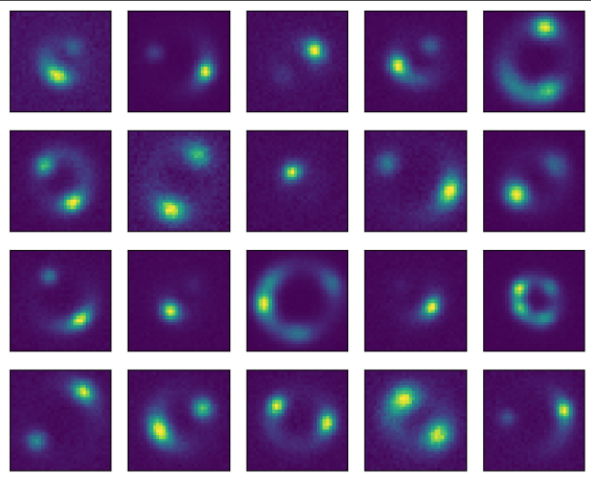
Figure 1: 20 randomly selected examples of $g$-band images in the test set used in the 5-parameter model. To mimic the lens light subtraction during traditional lens modeling, the lens light has not been added, so only the lensed source light is shown. The source magnitudes are $m_{s}=21$, which makes them appear less noisy than some of the images in Fig. 2, which have a larger variation in magnitude.

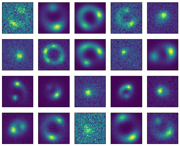
Figure 2: 20 randomly selected examples of $g$-band images in the test set used in the 12-parameter model. To mimic the lens light subtraction during traditional lens modeling, the lens light has not been added during the simulation phase, so only the lensed source light is shown. The source magnitudes in these images have a wide range: $18<m_{s}<25$. Due to the magnitude range, some fainter objects appear noisier than the images in Fig. 1.

5 Model Evaluation Diagnostics

For each model in this work, we performed multiple statistical and stability tests. The statistical checks include simulation-based calibration (SBC), which operates in parameter space [125, 91], and posterior predictive checks (PPCs), which operate in the observable/data space. We tested the model’s stability with respect to the random initialization of the network parameter weights and its generalization capacity.

5.1 Simulation-based Calibration

5.1.1 Posterior Coverage

For a model to be trustworthy, it must produce uncertainty estimates that are credible and well-calibrated. The posterior coverage measures how well-calibrated the predicted uncertainties of the posterior models are. For a posterior distribution to be well-calibrated, it must contain the true value $p\%$ of the time in $p\%$ of the posterior probability volume. For example, a posterior distribution with 68% (1$\sigma$) confidence intervals should contain the true value within those confidence intervals 68% of the time. Moreover, these uncertainties will have to be averaged across a large ensemble of lenses in a test set, as the estimated posteriors of a single lens image alone may not be indicative of the average performance of the model.

We present the model posterior coverage, which is calculated using the following steps:

1. Create a test set of 1000 lens images as described in § 4.

2. For each lens in the test set, use the trained posterior estimator to obtain an estimate of the posterior distribution of the model parameters for that particular lens by sampling the posterior estimator model.

3. From each posterior distribution, calculate parameter confidence intervals for that lens.

4. For each confidence interval, calculate the fraction of the lenses in the test set whose true parameter values fall within that confidence interval range.

5. For each parameter, plot the fraction of the lenses whose true parameter values fall within the confidence interval as a function of the confidence interval.

If the model’s posterior uncertainties are perfectly calibrated for the entire test ensemble, we expect the posterior coverage to follow the 1-1 line (Fig. 4). If the posterior coverage falls above the 1-1 line, it is underconfident because it overestimates the uncertainties, and a larger fraction of the test set’s true values fall within the given confidence interval than predicted by the model. Conversely, if it falls below the 1-1 line, it is overconfident and underestimates the true uncertainties.

5.1.2 Combined Distance Metric

In addition to calculating the posterior coverage for individual parameters, we calculate the distance metric from [135], defined as:

$$D(\bm{\theta}_{i})=(\bm{\theta_{i}}-\bm{\mu_{\theta_{i}}})\Sigma_{\textrm{data}}(\bm{\theta_{i}}-\bm{\mu_{\theta_{i}}})^{T},$$ (5.1)

where $\bm{\mu_{\theta_{i}}}$ is the vector of the means of the $i$-th lens’ posterior parameters and $\Sigma_{\textrm{data}}$ is the empirical covariance matrix for the training set parameters. $\bm{\theta_{i}}$ is a vector of parameter values of a posterior sample for the $i$-th lens. The distance metric $D(\bm{\theta}_{i})$ combines a vector of parameter values (e.g., from a posterior sample) into a single objective function that takes into account the covariance between different parameters.

5.1.3 Residuals

To characterize the statistical performance of the best-fit values over an ensemble of test images, we use the residuals. We calculate it as follows:

1. For each lens in the test set, we use our model/s to infer the lens parameter posteriors.

2. We then subtract the best-fit (maximum likelihood) parameter values from the true value of the lens parameters for each lens to obtain the residual.

3. For the case of a single-parameter fit, the plot shows the true posterior as a function of the residual. For the case of a multi-parameter fit, we plot the residuals for all lenses in the test set as a multidimensional (sometimes called a “corner” or “triangle”) plot.

We show 68% and 95% contours of the residuals (Fig. 8). The multi-parameter residual plots are similar to parameter covariance (“corner” or “triangle”) plots of an MCMC sampling analysis [18, 43, 84], which displays covarying scatter for every pair of parameters and a probability density of each parameter in some parameter space. The difference is that in an MCMC corner plot, each scatter point represents a posterior sample from the MCMC chain. However, in the plots described here, each scatter point represents the difference between the model’s best-fit estimate and the ground truth values of the parameters of one image in the test set.

The scatter characterizes the average best-fit point estimate of the model across the entire test ensemble and can be thought of as a multidimensional variant of the true-vs-predicted scatter plot visualization diagnostic that is common in machine learning literature. If the method is accurate (predicts the true value for every single lens), one expects a single point at (0,0). If the method produces systematically biased best-fit point estimates, we expect the scatter to shift away from the origin, and if the method is not precise, we expect a large scatter in the distribution.

We present this diagnostic plot for two reasons. First, if the models are systematically biased in a way that is correlated between any pair of parameters, we will be able to identify highly skewed (degenerate) contour plots for those pairs of parameters. It would not be possible to visualize correlated biases in true-vs-predicted scatter plots. Second, when plotting true-vs-predicted scatter plots for a large number of test images with their associated uncertainties, the visualization becomes cluttered, and it is difficult to discern structure in the inferences.

5.1.4 Rank Histogram

Simulation-based calibration [SBC; 125] tests are a general method of diagnosing and validating Bayesian inference methods based [35]. The SBC procedure is:

1. From the prior, we randomly generate $N$ independent parameter samples $\theta_{i}$.

2. We simulate observations of each lens image $X_{i}$.

3. From the trained NPE model, we obtain $M$ independent randomly chosen posterior samples $p_{m}(\theta_{i}|X_{i})$ from each of the $N$ posterior models.

4. For each NPE model, we count the number of samples of $p_{m}(\theta_{i}|X_{i})$ that fall below the corresponding true parameter value $\theta_{i}$. This number is the rank.

The main principle behind SBC is that if the trained posterior model is well-calibrated, the SBC ranks should be uniformly distributed between 0 and $N$. The reason for this is that samples from each of the randomly chosen posteriors should be distributed according to the prior. This corresponds to the claim that the $p\%$ confidence interval of this posterior model should contain the simulated value in $p\%$ of simulations for all values of $X$. Histograms of the SBC rank distributions serve as a diagnostic for checking if the posterior model is correctly computing the posterior. Deviations from uniformity in SBC rank histograms indicate how the computed posteriors are systemically biased. Specifically, if the histogram is:

• left-skewed: The posterior model is biased high compared to the true posterior and systematically overestimates the posterior mean.

• right-skewed: the posterior model is biased low compared to the true posterior and systematically underestimates the posterior mean.

• $\cup$-shaped: On average, the posterior model is narrower than the true posterior and systematically underestimates the uncertainty.

• $\cap$-shaped: On average, the model posterior is wider than the posterior model and systematically overestimates the uncertainty.

In addition to the visual indications of bias listed above, we plot the 99%-confidence interval of a uniform distribution given the number of samples provided. For a uniform distribution, we expect 1 out of 100 histogram bars to lie outside the confidence interval. In the SBC plots, this is indicated by a gray region (Fig.13, top row).

5.1.5 Rank Cumulative Distribution Function (CDF)

The rank CDF is another method of presenting the rank information from § 5.1.4. If the posterior is perfectly calibrated, one expects a perfectly diagonal CDF, which is equivalent to a uniformly distributed rank in the histogram. We plot the 99%-confidence interval of a uniform distribution given the number of samples provided, indicated by a gray region (Fig.13, bottom row). If the posterior model is systematically biased high (low), the rank CDF will deviate above (below) the diagonal line. If the posterior model systematically overestimates (underestimates) the uncertainty, the CDF will resemble a diagonal ’S’ (inverted ’S’) shape. The choice of visualization of ranks involves some trade-offs. CDFs do not depend on the choice of histogram binning size [91]. The plots also allow for multiple parameter rank CDFs to be overlaid on the same plot, resulting in more compact visuals compared to the histogram. However, it is often easier to visually identify model pathologies from the rank histograms. Due to these trade-offs, we opt to show both rank histograms and CDFs for our models.

5.2 Posterior Predictive Checks (PPCs)

Posterior predictive checks [44] are a commonly used diagnostic (Fig. 3, top row). While they have been found lacking as a validation metric [88] for SBI, PPCs can be used as a starting point for diagnosing NPE performance by providing visual intuition about potential biases in the model’s inference. These show how the best-fit parameters for a given model are reflected in the reconstructed data model of the lensing system.

5.3 Stability Tests

Network weights are randomly initialized, which allows variation in results amongst models trained on the same data [107]. While the effects of initialization don’t generally produce a large variance in the performance [107], it is not difficult to fortuitously pick random seeds that perform significantly differently from the average. While the use of those seeds does not mean the results of those models are invalid, their performance may not be representative of the typical performance of that particular deep learning architecture, making it challenging to determine a model’s true performance. Therefore, it is important to diagnose the stability across multiple seeds. We train NPE models with three different seeds. We do not perform this diagnostic for the BNN models because the computation is prohibitively expensive, and BNNs are not the primary focus of this study.

6 Results

We present the results of NPE and BNN model inference with three levels of complexity: a baseline 1-parameter model where one lens parameter is varied and inferred; a 5-parameter model where five lens parameters are varied; and a 12-parameter model that varies the seven lens-plane parameters and five source-plane parameters.

6.1 1-parameter Model: Varying One Lens Parameter

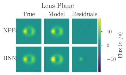
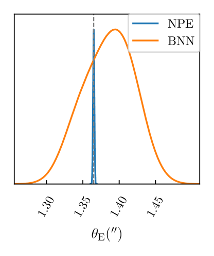
Figure 3: Performance for a single image in the 1-parameter NPE and BNN models. Top: the posterior predictive check for the lens plane image for the NPE (upper row) and the BNN (lower row) models, which includes the true image, the image predicted by each method, and the residual between the true and the predicted image for this test object. Bottom: inferred posterior of the Einstein radius $\theta_{E}$ for the NPE (blue) and BNN (orange) models. We provide more examples in Appendix B.

We use the 1-parameter model as a starting point for studying training regimes and as a baseline for comparison with models of greater complexity. In this problem, as described in § 3 and § 4, we vary the Einstein radius while leaving other parameters fixed. We trained the models on 200,000 images in which the Einstein radius ranged from 0.3 to 4.0 arcsec. We used 100 hidden features and 10 transformations for the NPE model. Fig. 3 shows the posterior distribution of $\theta_{E}$ inferred by both the NPE and BNN model for a single lensed image in the test set. This figure also shows a comparison of the posterior predictive check for the NPE and BNN models: the true image, the image reconstructed with the best-fit parameters, and the residuals between the true and reconstructed image. In this simple problem, both NPE and BNN models are extremely accurate and precise, inferring the true $\theta_{E}$ value with $\sim 10^{-3}$ arcsec and $\sim 10^{-2}$ arcsec $68\%$ uncertainties, respectively. However, the NPE method is both more accurate and $\sim 10$ times more precise than the BNN model.

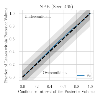
Figure 4: Posterior coverage of the 1-parameter NPE (left, blue) and BNN (right, orange) models computed on the test set (solid). The 1-1 line (black, dashed) indicates perfect uncertainty calibration. The gray regions indicate thresholds of 10% (dark gray) and 20% (light gray) uncertainty miscalibration.

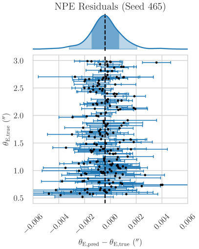
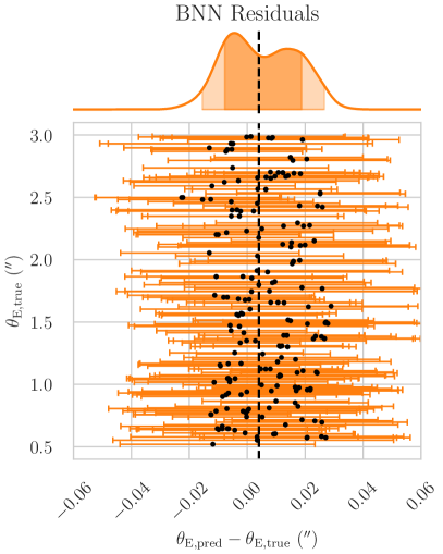
Figure 5: Residuals of the inferred posterior of the Einstein radius $\theta_{\mathrm{E}}$ in the 1-parameter NPE (blue, left) and BNN (orange, right) models for 200 images randomly selected from the test set. The error bar represents the 68% uncertainty in $\theta_{\mathrm{E}}$ for each image. Above the scatter plot of the residuals, the marginal distribution of best-fit values for the full test set of 1000 is shown. The 68% and 95% scatter in best-fit values are indicated by the dark and lighter-shaded regions, respectively. The NPE model random seed for weight initialization is set to $465$.

We quantify model performance primarily in two ways. First, we study the posterior coverage (§ 5.1.1). Fig. 4 shows the posterior coverage for the NPE and BNN models. The NPE method is slightly underconfident (within 5% of perfect calibration), while the BNN model is extremely underconfident. Second, the residuals show the deviations of posteriors from the true parameter for 1000 test images. The lower panels of Fig. 5 show the scatter of residuals in point values with error bars (68% confidence intervals) for 200 randomly selected test images. We also show the distribution of residuals in the upper panel of that figure. We perform kernel density estimation on the posterior distributions with a bandwidth calculated using Scott’s rule [118], with the 68% and 95% confidence intervals in the distribution of the residuals. The 68% confidence intervals in the residuals are $\sim 10^{-3}$ arcsec for the NPE model and $\sim 1-2\times 10^{-2}$ arcsec for the BNN model, with the predicted model uncertainties in the same regime. This is in agreement with the single-image example in Fig.  3 and further validates that specific example as representative of the typical performance of both models. The distribution of residuals in the BNN model (Fig. 5, right) appears to exhibit bimodality, pointing to non-Gaussian systematic uncertainty in the BNN model point estimates.

To study model stability, we change the random seed initialization on the NPE model. We present the main results of those diagnostics in Appendix B.1.

6.2 5-parameter Model: Varying Five Lens Parameters

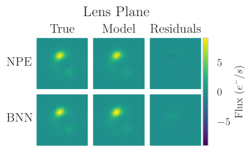
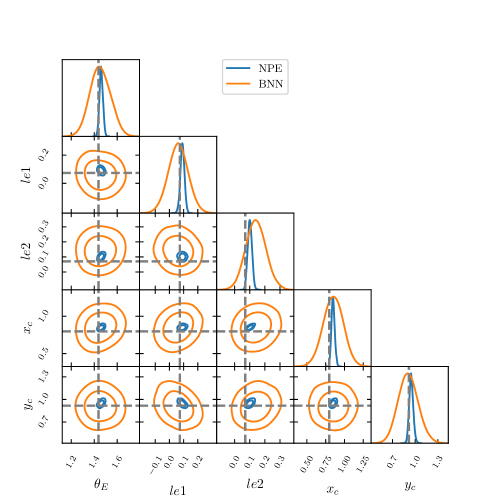
Figure 6: Performance of the 5-parameter NPE and BNN models for a single lensing system from the test set. Top: the posterior predictive check for the lens plane images for the NPE (upper row) and the BNN (lower row) models, which includes the true image, the image predicted, and the residual between the true and the predicted image. Bottom: inferred posterior distributions of five parameters for the NPE (blue) and BNN (orange) models. The value and 68% uncertainty listed at the top of each column are for the NPE model. The gray dashed line indicates the true value. We provide more examples in Appendix B.

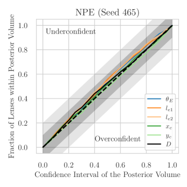
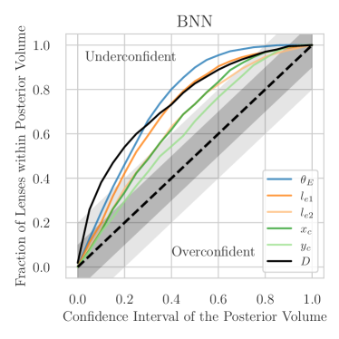
Figure 7: Posterior coverage for the five-parameter NPE (left) and BNN (right) models for the test set. The 1-to-1 line (dashed, black) indicates perfect uncertainty calibration. The gray regions indicate thresholds of 10% (dark gray) and 20% (light gray) uncertainty miscalibration. The solid black line represents the distance metric described in Eqn. 5.1. The NPE model random seed for weight initialization is set to $465$.

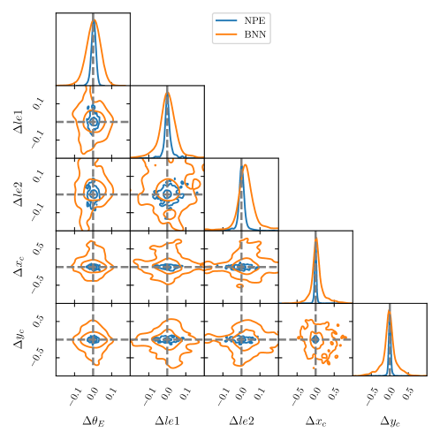
Figure 8: Residuals of the inferred posteriors for the 5-parameter NPE (blue) and BNN (orange) models for 1000 images from the test set. The average zero residual is represented by the gray dashed line. The same sample is used in the NPE model and the BNN model. The contours represent approximate $68$th and $95$th percentile uncertainties in the scatter. The NPE model shown here is for the case in which the random seed for neural network initialization has been set to $465$.

The 5-parameter model has more complexity than the 1-parameter model: aside from $\theta_{\mathrm{E}}$, there are two additional parameters for lens eccentricity moduli ($l_{e1}$, $l_{e2}$) and two additional parameters for the positional offset between the lens and the source ($x_{\mathrm{c}}$, $y_{\mathrm{c}}$). We trained the models on 400,000 images with parameter distributions shown in Table 5. During training, the neural density estimator was instantiated with 120 hidden features and 20 transforms for the MAF. We evaluated the performance on a test set of 1000 lenses generated using the priors recorded in Table 5. Fig. 6 shows the results of inference on a single image drawn randomly from the test set — a corner plot of posteriors and the posterior predictive check for the model-based lens reconstruction. Table 6 summarizes the results for the 1000-sample ensemble.

The performance of the NPE and BNN models on the 5-parameter model is similar to that on the 1-parameter model. First, the NPE model produces significantly smaller uncertainties than does the BNN model. Compared to the 1-parameter model, the average uncertainty in $\theta_{\mathrm{E}}$ is about $\sim 0.02$ arcsec for the NPE, and it is $\sim 0.08$ arcsec for the BNN model, compared to $\sim 10^{-3}$ arcsec and $\sim 10^{-2}$ arcsec $68\%$, respectively, in the 1-parameter model. Unlike the 1-parameter model, the BNN uncertainties are $\sim 1-5$ times larger than the NPE model, rather than 10 times larger, as in the 1-parameter model. The residuals in Fig. 8 show that the NPE and BNN models are both unbiased. The median values are consistent with zero within the 68% scatter intervals (Table 6). However, the 68% scatter is two to three times wider in the BNN model than in the NPE model, showing that the BNN model is less precise than the NPE. There appear to be no degeneracies or correlations amongst the parameter residuals. The posterior coverage in Fig. 7 exhibits similar patterns as for the 1-parameter model. The NPE model uncertainties are well calibrated, whereas the BNN uncertainties are underconfident for every parameter in the model — albeit slightly less so for the position parameters.

We also explore model stability for the 5-parameter model. We find that the model is stable with respect to different random seed initializations of the network weight parameters. Details of that exploration can be found in Appendix B.2.

6.3 12-parameter model: Varying Five Lens and Seven Source Parameters

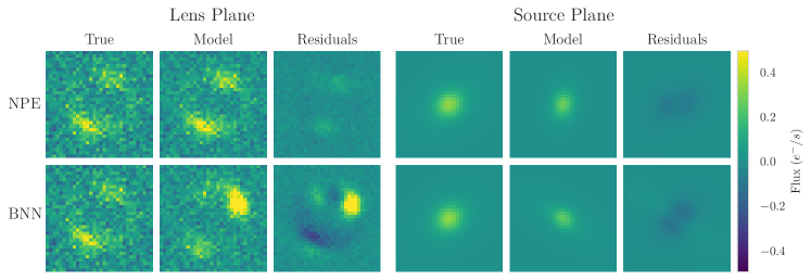
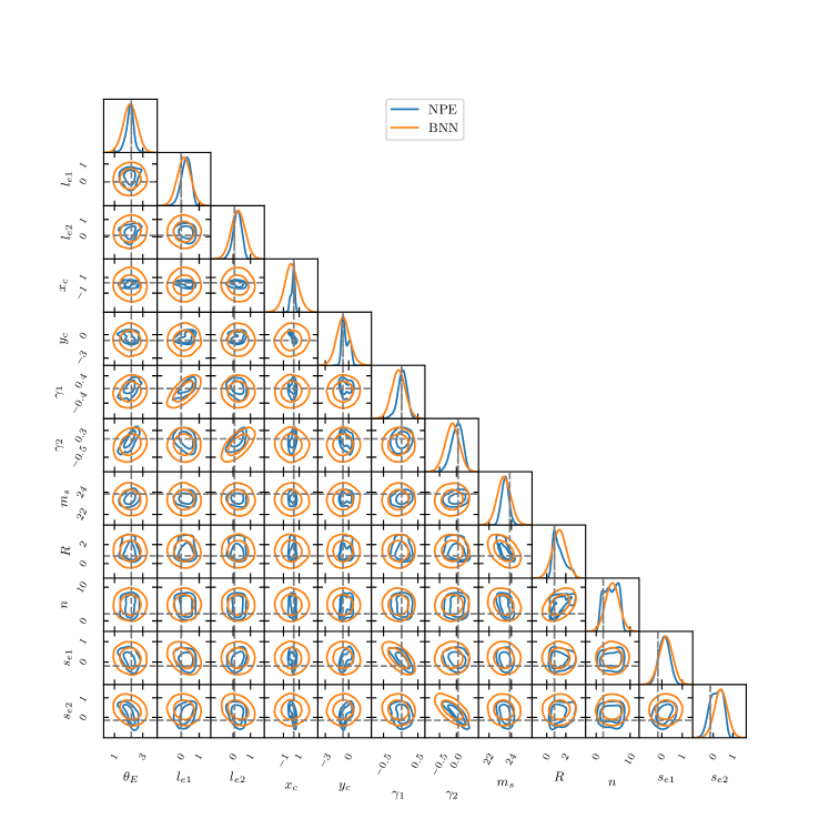
Figure 9: Performance of the 12-parameter NPE and BNN models for a single lensing system from the test set. Top: the posterior predictive check for the lens plane and the source plane, which includes the true image, the image predicted by NPE (top) and the BNN (bottom), and the residual between the true and the predicted image. Bottom: inferred posterior distributions of 12 parameters for the NPE (blue) and BNN (orange) models. The true value is indicated by the gray dashed line. We provide more examples in Appendix B.

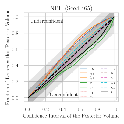
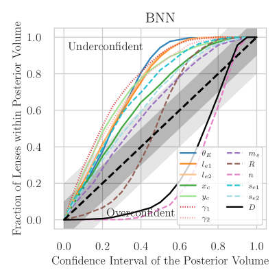
Figure 10: Posterior coverage of 12-parameter NPE (left) and BNN (right) models for the test set. The 1-to-1 line indicates perfect uncertainty calibration and is indicated by a dashed black line. The gray regions indicate thresholds of 10% (dark gray) and 20% (light gray) uncertainty miscalibration. The solid black line shows the combined distance metric $D$ (Eqn. 5.1). The lens parameter coverage, source parameter coverage, and shear parameter coverage are indicated by solid, dashed, and dotted lines, respectively. The NPE model random seed for weight initialization is set to $465$.

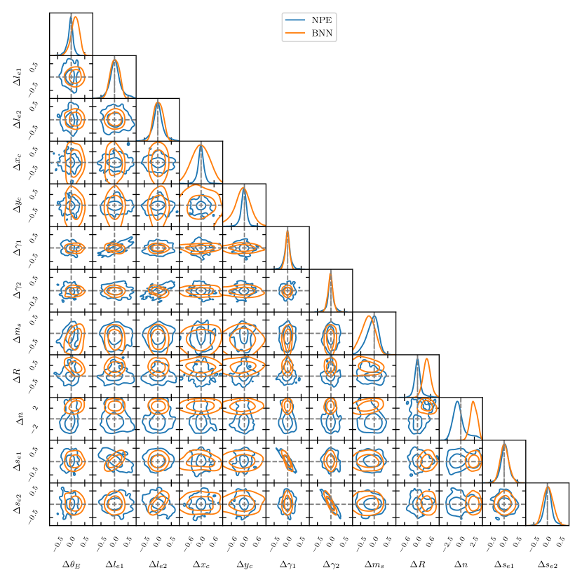
Figure 11: Residuals of the inferred posteriors of the parameters for the 12-parameter NPE (blue) and BNN (orange) models for 1000 images from the test set. Zero residuals are indicated by gray dashed lines. The contours represent 68th- and 95th- percentile uncertainties in the scatter. The NPE model is for the random seed set to $465$.

The 12-parameter model is the most complex model that we consider. In addition to the five lens parameters discussed in § 6.2, we model two parameters for the external shear ($\gamma_{1},\gamma_{2}$) and five parameters for the source light distribution ($m_{s}$, $R$, $n$, $s_{e1}$, $s_{e2}$). We trained the models on 800,000 images with parameter distributions shown in Table 5. For training, the neural density estimator was instantiated with 400 hidden features and 20 transforms for the MAF. We primarily evaluated the performance on a test set of 1000 lenses. Fig. 9 shows the inferred posterior distributions and model reconstruction for a single image from the test set.

The NPE model was more accurate and precise than the BNN model, inferring smaller uncertainties on the same test image by a factor of $\sim$1-3. This is similar to the trends exhibited in the 1- and 5-parameter models. The posterior coverage of the models (Fig. 10) shows that the NPE outperforms the BNN model with respect to uncertainty calibration: for the NPE model, the coverage for all parameters is within 10% of perfect calibration. The BNN model is underconfident for every parameter except $R$ and $n$, for which it is overconfident. The BNN’s posterior coverages for $R$ and $n$ exhibit ’S’-shaped coverage, which is usually an indication that the inferred posteriors are failing to accurately capture the ground truth values. The parameters $R$ and $n$ are source light parameters that produce extended lensing observables that map from the source plane to the lens plane in less straightforward ways. Inferring these parameters may be more challenging as a result. We hypothesize that the NPE model’s better performance is due to MAF’s inherently more flexible density estimators than the Gaussian densities of the BNN, as MAFs are proven to be universal approximators, capable of representing any probability distribution given certain reasonable conditions [104]. Given enough training data, MAFs can more accurately estimate the true posterior distribution of the lens parameters.

The residuals in Fig. 11 show that the NPE model outperforms the BNN model in accuracy for all parameters. The NPE model is not highly accurate for $n$, but it is more accurate than the BNN model. For ($s_{e_{1}}$, $s_{e_{2}}$), ($l_{e_{1}}$, $l_{e_{2}}$), and ($\gamma_{1}$, $\gamma_{2}$), both NPE and BNN models are similarly precise and produce residuals of similar size. For those parameters, the NPE model residuals also have a longer tail than the BNN model, with slightly wider 95% contours than the BNN. One interpretation for the difference in accuracy between the 5-parameter model and the 12-parameter model is related to the training set size and the parameter space volume. Despite increasing the training set size for the 12-parameter model to 800,000 images, the parameter space volume increases exponentially with the number of dimensions, outpacing the increase in training set size. Hence, the average sampling distance between points in the 12-parameter space is exponentially larger than that of the 1- and 5-parameter spaces, resulting in a less accurate model fit for the 12-parameter model. Despite the NPE method being more flexible than the BNN, it is still constrained by the size of the training set. Due to computational constraints, we were unable to increase the training set size above 800k images. This prohibits increasing the training set size to that required to maintain the same sampling distance as the 1- or even 5-parameter model; this is not the same distance metric as Eqn. 5.1.

For the position parameters ($x_{\mathrm{c}}$, $y_{\mathrm{c}}$), both NPE and BNN models were accurate and unbiased. However, the BNN residuals exhibit significantly larger scatter (lower precision) than the NPE residuals, with the BNN’s 68% uncertainties being similar in size to the NPE model’s 95% uncertainties. The NPE model is unbiased for all the parameters except for $n$, which it underestimates by $\sim 0.2$, although it is within the 68% uncertainties. The BNN, however, is systematically biased for four parameters $\theta_{\mathrm{E}}$, $m_{s}$, $R$, and $n$. The BNN overestimates $\theta_{\mathrm{E}}$ and underestimates $m_{s}$, as evidenced by the peaks of the residuals shifted away from zero. The BNN performed worst on $R$ and $n$, overestimating the true values for more than 95% of the test set. The BNN also overestimates $R$ by $>0.4$ arcsec and $n$ by 2.4. This poor performance is also reflected in the ’S’-shaped posterior coverage for these parameters in Fig. 10. As hypothesized earlier, these are source light parameters, which have non-linear mappings to the observed image plane. The BNN model relies on normal distributions for its parameters and may not have enough flexibility to capture the true posterior distribution accurately. In comparison, the NPE was more accurate and precise in inferring the best-fit parameter values for all these parameters.

Some parameters demonstrate correlations in their residuals. For both the NPE and BNN models, the residuals of $\theta_{\mathrm{E}}$  are slightly positively correlated with residuals of $m_{s}$. For both models, the residuals of $l_{e_{1}}$ and $l_{e_{2}}$ and $s_{e_{1}}$ and $s_{e_{2}}$ are positively correlated with residuals of $\gamma_{1}$ and $\gamma_{2}$. However, the BNN (NPE) residuals for the lens eccentricity parameters are positively (negatively) correlated with the source eccentricity parameters. This parameter degeneracy is well-documented in strong lens modeling literature [15, 132]. However, the uncertainties and residuals of the eccentricities and shear may be correlated because we are jointly inferring them: offsets or errors in one parameter could be accounted for by offsets in another.

Table 6: Summary of results comparing the NPE and BNN model performance for the 1-, 5- and 12-parameter models for the test set. The table values are the average central values and the 68% scatter in the residuals for each parameter across 1000 lenses.

	1-param Model		5-param Model		12-param Model
Param	NPE	BNN	NPE	BNN	NPE	BNN
$\Delta$$\theta_{\mathrm{E}}$ (′′)	$-0.0004\pm{0.0011}$	$0.004^{+0.015}_{-0.012}$	$0.002^{+0.013}_{-0.011}$	$0.002^{+0.040}_{-0.035}$	$-0.046^{+0.13}_{-0.078}$	$0.14^{+0.17}_{-0.13}$
$\Delta$ $l_{e1}$	-	-	$0.003^{+0.012}_{-0.017}$	$0.002\pm 0.066$	$0.03^{+0.16}_{-0.20}$	$0.02\pm 0.16$
$\Delta$$l_{e2}$	-	-	$0.001\pm 0.030$	$0.028^{+0.034}_{-0.047}$	$0.00\pm 0.20$	$0.02\pm 0.16$
$\Delta$$x_{\mathrm{c}}$ (′′)	-	-	$0.004^{+0.018}_{-0.030}$	$0.043^{+0.093}_{-0.14}$	$-0.01\pm 0.24$	$-0.03\pm 0.42$
$\Delta$$y_{\mathrm{c}}$ (′′)	-	-	$-0.006^{+0.031}_{-0.026}$	$-0.02\pm 0.20$	$-0.03^{+0.14}_{-0.12}$	$-0.11^{+0.42}_{-0.34}$
$\Delta$$\gamma_{1}$	-	-	-	-	$-0.01\pm 0.12$	$-0.0095\pm 0.079$
$\Delta$$\gamma_{2}$	-	-	-	-	$-0.01\pm 0.12$	$-0.020\pm 0.094$
$\Delta$$m_{s}$	-	-	-	-	$-0.08^{+0.25}_{-0.17}$	$-0.24^{+0.29}_{-0.23}$
$\Delta$$R$ (′′)	-	-	-	-	$0.041^{+0.090}_{-0.19}$	$0.43\pm 0.18$
$\Delta$$n$	-	-	-	-	$-0.23^{+0.59}_{-1.4}$	$2.38^{+0.69}_{-0.63}$
$\Delta$$s_{e1}$	-	-	-	-	$0.03\pm 0.17$	$0.01^{+0.15}_{-0.17}$
$\Delta$$s_{e2}$	-	-	-	-	$0.02\pm 0.17$	$0.03^{+0.17}_{-0.20}$

The NPE model exhibits slight variations in uncertainty calibration for three different weight initializations. This may be explained by the increase in average sampling distance between training data points in the 12-parameter space compared to the 1- and 5-parameter spaces, which results in greater uncertainty in model fitting. $m_{s}$ appears to be biased high, and $n$ appears to be biased low for all three seeds.

7 Discussion

In this section, we discuss challenges in model development and evaluation for NPE models.

7.1 Adopting Sequential SBI for Follow-up Studies

The goal of this work is to efficiently infer astrophysical parameters from a large sample of lensing images. This procedure requires amortization — the fast training and optimization of a model. Sequential methods, however, require a model to be trained each time new results are obtained (§ 3.2.5). However, we can imagine using sequential methods to follow up on a small sub-sample of lensing images to refine the NPE model. For example, after an initial analysis using NPE and ancillary observations (e.g., lenses where we have access to spectroscopic data), one could identify a smaller sub-sample of information-rich lenses — e.g., quadruply-imaged lenses or time-delay lenses — that we would like to refine the posterior estimates of, we can perform SNPE on those lenses by using the posteriors obtained from NPE in this work as a proposal prior for subsequent rounds of inference, thereby ensuring that no computation is wasted.

7.2 Increasing Modeling Complexity

In this study, the most complex model has 12 physics parameters. This level of complexity is appropriate for the majority of lenses we expect to discover in ground-based imaging data — i.e., single-lens, single-source galaxy-galaxy lenses with $\sim$1-arcsec resolution [e.g., 3, 73]. However, more complicated lens system models, such as cluster-scale lenses, multi-source-plane lenses, and lens subhaloes, could require $\sim$30-50 parameters [e.g., 89]. Moreover, even with high-resolution, lower-noise space-based imaging (e.g., Roman, Euclid, JWST), the dimensionality of the model remains a challenge for SBI methods.

Generally, SNPE appears to scale well to high-dimensional observations, but its scaling to parameter space dimensions greater than 30 is more challenging [48]. Given that the difficulty of estimating full posteriors scales exponentially with dimensionality, this is an inherent challenge for all approaches that aim at full inference. The dimensionality of the observation refers to the dimensionality of the dataset: in our work, the dimensionality of our observations is 1024, corresponding to the number of pixels in each image. Advances in both SBI and density estimation techniques have overcome the limitations of the curse of dimensionality suffered by classical ABC techniques; although SBI doesn’t yet have statistical guarantees, which are especially crucial for trustworthiness when these models are applied to real data. However, further advances must be made for SBI techniques to scale for models in very high-dimensional spaces. In addition, the validation techniques used to ensure the credibility of the model also need to scale up to that number of parameters.

Advancements in recent years may enable NPE methods to continue scaling to higher-dimensionality problems in the future. First, many simulators provide only pairs of input data and parameters $(X,\theta)$. When simulators provide more information — e.g., the score $\nabla_{\theta}p(X|\theta)$, which is the gradient of the likelihood with respect to the parameters of interest — models can be more performant and more efficiently trained. This has been applied to strong lensing analyses in the form of a proof-of-concept analysis of dark matter subhalo population properties in strong lenses [24].

Second, combining SBI with hierarchical modeling may efficiently provide greater constraining power when population-level (i.e., cosmological) parameters like the cosmic matter density $\Omega_{m}$ and the dark energy equation of state $w$ are the goal of the inference. Hierarchicality in SBI has been studied in a few strong lensing applications [135, 136, 64], and it has been directly implemented with neural posterior estimation [113, 53].

7.3 Model Calibration

Post-training calibration in machine learning models is an actively studied field, with much of the literature focused on calibrating neural network predictions in a classification or regression task [51]. In this work, we did not apply post-training model calibration to evaluate or enhance performance. Calibration of SBI models in an astrophysical context is largely unexplored, although beta calibration [76] has been used to calibrate BNN models to predict cosmological parameters from Cosmic Microwave Background maps [56]. Conformal methods [7, 134] offer a promising calibration technique because they provide guarantees regarding the coverage, provided that the test set is independent and identically distributed to the validation set used for the calibration. However, the calibrated model, while valid, predicts the same uncertainties for all test set data and is unable to predict larger uncertainties for data within the test set that have higher risk — such as noisy images. While there has been recent work to make conformal prediction both valid and discriminative [86], it is unclear how this may be combined with existing SBI methods of uncertainty prediction.

8 Conclusion

In this work, we explore the capacity of NPE methods to model large numbers of strong lensing systems at various degrees of complexity, which is marked by the number of parameters in the model — one, five, and 12. We compare NPE to BNN because they are one of the few approaches that can quickly predict model parameters from images. Traditional lens modeling algorithms are too inefficient to infer parameters from large numbers of lenses. We use SBC’s and PPC’s to study the validity of the NPE and BNN models. We also study the stability of these models with respect to network weight initialization. The comprehensiveness of these experiments and diagnostics is a contribution to SBI applications in astrophysics contexts.

Our main results are:

1. Both NPEs and BNNs provide informative inferred posterior distributions of lens parameters in experiments with noisy ground-based galaxy-galaxy lenses.

2. Due to their amortized nature, the NPE and BNN models infer the posterior densities of thousands of lens systems in minutes. This meets the scaling requirement for tens to hundreds of thousands of lens systems that are projected to be discovered in future survey data. For the 12-parameter model, both NPE and BNN models took about six hours to train. In comparison, a conventional MCMC fit would take around the order of an hour per lens system.

3. This work demonstrates of the use of Masked Autoregressive Flows (MAF) for lens parameter posterior density estimation. Previous work used mixture density models [80, 81].

4. We found that the NPE model uncertainties are generally more well-calibrated than the BNN model uncertainties. In this work, the BNN models tend to be underconfident — overpredicting the uncertainties of the test images. One potential method to improve the uncertainty calibration of the BNN model is to increase the number of Gaussian components in the model weights. However, this comes with the trade-off of a steep computational cost increase because each additional Gaussian component requires two additional free parameters to be trained for every weight in the network.

5. The effect of random seed initialization in NPEs is subdominant to the model uncertainties in the 5- and 12-parameter models, implying that the choice of model will not significantly impact the results (see Appendix B). In the 1-parameter model, the choice of random seed results in a $\sim 0.1\%$ uncertainty, which is on the same order of magnitude as the uncertainties from the posterior itself. However, this is unlikely to impact the modeling of real lenses in practice, as achieving a $\sim 0.1\%$ uncertainty estimate is only possible in the 1-parameter model, which is too simple to accurately model real lenses. In practice, real lenses have uncertainties on the order of 5% [115].

6. NPE methods do not yet come with statistical guarantees. Therefore, it’s critical that applications are accompanied by diagnostics to assess model calibration and stability. This includes assessing the following: (1) both maximum-likelihood point estimates and uncertainty estimates are unbiased and well-calibrated when averaged across a large ensemble of data; (2) model performance does not exhibit large variation with the choice of random seeds for weight initialization. These diagnostics are essential for showing that a model produces reliable and reproducible results.

This work presents another step in the study of SBI methods, which have advanced in recent years due to developments in deep learning, as well as exponential gains in computational efficiency. There are multiple avenues for further exploration and development — both in fundamental algorithm challenges and in the application to strong gravitational lensing and other astrophysical probes. First, for algorithm development, as discussed in § 7, SBI methods that leverage not only the training data but additional information that characterizes the latent process of the simulators — e.g., the score — may increase model performance. Second, the potential performance improvements and computational trade-offs from ensembling large numbers of SBI models should also be investigated in more detail. Third, the lack of statistical guarantees and fully interpretable uncertainties hinders the trustworthiness of these methods. Well-motivated diagnostics like SBC present the best tools for evaluating SBI model fitness. Aside from diagnostics, post-calibration techniques may provide a near-term partial substitute for formal theoretical guarantees.

Appendix A Correction to Magnitude Calculation

While finalizing this manuscript, we discovered a bug in the simulation code. When the background noise was simulated, the sky brightness was not correctly converted from magnitude to counts per second. The consequence of this bug is that the average root mean square noise per pixel in the simulation is lower than it should have been by a factor of $\sim 1.6$: this factor leads to $\sim 0.08$ counts per pixel instead of $\sim 0.13$ counts per pixel. This does not significantly affect the results or conclusions of this work because the RMS noise is typically an order of magnitude lower or less compared to the average lensing signal in the simulated images on all the models.

Appendix B Experiments for Model Stability

We study NPE model stability for the three levels of problem complexity in this work: 1-parameter, 5-parameter, and 12-parameter models. We initialized model weights with three different random seeds (42, 465, and 839) to study the variation in model performance on a single test data set with priors within the range of the training set. Generally, the diagnostics indicate that the models are stable and reliable.

Table 7: Parameter distributions used to generate the training and test set. The parameters relevant to each model are indicated under the Models column. The full list of model parameters is as follows. For the lens mass, we use the SIE mass profile, Einstein radius $\theta_{\mathrm{E}}$, eccentricity components $l_{e1}$ and $l_{e1}$, and lens-source offset positions $x_{c}$ and $y_{c}$. For the lens environment, we use the two components of the external shear $\gamma_{1}$ and $\gamma_{2}$. For the source light, we use a Sersic profile with apparent magnitude $m_{s}$, half-light radius $R$, Sersic index $n$, and eccentricity components $s_{e1}$ and $s_{e2}$. Uniform distributions are denoted by $\mathcal{U}\mathrm{(minimum,maximum)}$, Normal distributions are denoted by $\mathcal{N}\mathrm{(mean,standard\ deviation)}$, and lognormal distributions are denoted by $\mathcal{N_{\log}}\mathrm{(mean,standard\ deviation)}$.

Parameters	Models	Training	Test
Lens Parameters
$\theta_{\mathrm{E}}$  (′′)	1,5,12	$\mathcal{U}(0.3,4.0)$	$\mathcal{U}(0.5,3.0)$
$l_{e1}$	5,12	$\mathcal{U}(-0.8,0.8)$	$\mathcal{U}(-0.2,0.2)$
$l_{e2}$	5,12	$\mathcal{U}(-0.8,0.8)$	$\mathcal{U}(-0.2,0.2)$
$x_{\mathrm{c}}$ (′′)	5,12	$\mathcal{U}(-2,2)$	$\mathcal{U}(-1,1)$
$y_{\mathrm{c}}$ (′′)	5,12	$\mathcal{U}(-2,2)$	$\mathcal{U}(-1,1)$
Lens Environment Parameters
$\gamma_{1}$	12	$\mathcal{U}(-0.8,0.8)$	$\mathcal{U}(-0.05,0.05)$
$\gamma_{2}$	12	$\mathcal{U}(-0.8,0.8)$	$\mathcal{U}(-0.05,0.05)$
Source Light Parameters
$m_{s}$	12	$\mathcal{U}(18,25)$	$\mathcal{U}(19,24)$
$R$ (′′)	12	$\mathcal{U}(0.1,3.0)$	$\mathcal{U}(0.5,1.0)$
$n$	12	$\mathcal{U}(0.5,8.0)$	$\mathcal{U}(2,4)$
$s_{e1}$	12	$\mathcal{U}(-0.8,0.8)$	$\mathcal{U}(-0.2,0.2)$
$s_{e2}$	12	$\mathcal{U}(-0.8,0.8)$	$\mathcal{U}(-0.2,0.2)$

B.1 1-parameter Model

First, regarding stability for the 1-parameter model, variations in model performance on $\theta_{E}$ were $\sim 10^{-3}$ arcsec ($\sim 0.1\%$) — the same order of magnitude of the model uncertainties. Fig. 14 shows residuals for the different seed models on the same test images. It is undesirable for the choice of random seed to significantly impact the model’s posterior predictions. However, this is an edge case because a $\sim 10^{-3}$-arcsec modeling uncertainty is only achievable for extremely constrained and unrealistic models, such as this 1-parameter model. In practice, modeling uncertainties for $\theta_{E}$ in the most optimal real-world cases — i.e., high-resolution space-based images of simple lens systems [115] — are on the order of 5%. The residuals for the 1-parameter model indicate that there may be a stochastic noise floor caused by weight initialization and that the uncertainty of this noise floor is on the order of $\sim$0.1%. The results show that given a sufficiently constrained model, it is possible to attain the precision and accuracy level up to the level of this noise floor. It may be possible to lower the noise floor via ensembling of model results to average out the noise. We discuss this in § 7.

We find that the NPE model is well-calibrated for each of the random seeds: the rank histograms and the accompanying cumulative distribution functions (Fig. 13), along with the posterior coverages (Fig. 14), show that one model (seed 465) is almost perfectly calibrated and that two models (seeds 42 and 839) are slightly underconfident. All three models in Fig. 13 exhibit slight $\cap$-shaped distributions in the rank histograms, indicating that the posterior models slightly overestimate the true posterior uncertainty. The rank histogram for the seed 42 model skews slightly to the left, indicating a slight bias towards lower values compared to the true posterior (underestimation). In comparison, the seed 465 model skews slightly to the right, indicating a slight systematic bias towards higher values (overestimation). These variations are not readily perceptible in the residual plots (Fig. 12) or the posterior coverage plot (Fig. 14).

Figure 12: Residuals of the inferred posterior of the Einstein radius $\theta_{\mathrm{E}}$ in the 1-parameter model for the NPE model, with three different seeds — 42 (left), 465 (middle), and 839 (right) for the network weight initialization for 200 images randomly selected from the test set. The error bar represents the 68% uncertainty in $\theta_{\mathrm{E}}$ for each image. Above the scatter plot of the residuals, the marginal distribution of best-fit values for the full test set of 1000 is shown. The 68% and 95% scatter in best-fit values are indicated by the dark and lighter-shaded regions, respectively. This is similar to the Fig. 5.

Figure 13: Rank histograms (top) and cumulative density functions (bottom) for the 1-parameter model with seeds 42 (left), 465 (middle), and 839 (right). We discuss the plots in § 6.1. In the rank histograms, the gray region indicates uniformity. In the CDFs, the gray regions indicate the 99% confidence interval of a uniform distribution given the number of samples provided.

.

Figure 14: Posterior coverage of the 1-parameter NPE and BNN models computed on the test set (solid). The NPE models are initialised with three seeds — 42, 465, and 839. The 1-1 line (black, dashed) indicates perfect uncertainty calibration. The gray regions indicate thresholds of 10% (dark gray) and 20% (light gray) uncertainty miscalibration.

B.2 5-parameter Model

The 5-parameter model is well-calibrated or nearly well-calibrated for most of the five parameters for all three seeds. For seed 42, the model is slightly miscalibrated for $\theta_{\mathrm{E}}$, $l_{e2}$, and $y_{c}$. For seeds 465 and 839, the models appears to be well-calibrated for all parameters. This is reflected in the rank histograms (Fig. 15) and CDFs (Fig. 16): the rank bins are consistent with a uniform distribution, where only one or fewer bins lie outside the grey 99% confidence region. Using the combined distance metric (Eqn. 5.1) as a proxy for the overall uncertainty calibration across all five parameters, we find that the seed 42 model is just slightly overconfident, the seed 465 model is almost perfectly calibrated, and the seed 839 model is just slightly underconfident. Such slight calibration differences are unlikely to be the most significant source of uncertainty in real-life applications. Still, it highlights the importance of evaluating the effects of the random weight initialization on the performance and stability of deep learning models.

Figure 15: Rank histograms for the 5-parameter NPE model with seeds 42, 465, and 839 (top, middle, bottom) for the weight initialization. The gray region indicates uniformity.

Figure 16: CDFs for the 5-parameter NPE model for seeds 42, 465, and 839. The gray regions indicate the 99% confidence interval of a uniform distribution given the number of samples provided.

Figure 17: Posterior coverage and the combined distance metric for the 5-parameter NPE models on the test set (first row) with three different seeds for the network weight initialization — 42 (left), 465 (middle), and 839 (right). The 1-1 line (black, dashed) indicates perfect uncertainty calibration. The gray contours indicate regions of 10% (dark gray) and 20% (light gray) uncertainty miscalibration.

B.3 12-parameter Model

For the 12-parameter model, according to the posterior coverage (Fig. 18), the rank histograms and the CDFs, our models exhibit slight variations in uncertainty calibration between seeds. These variations are larger than that of the 5-parameter model. For example, the least well-calibrated parameter across the three seeds in the 5-parameter model is the $\theta_{\mathrm{E}}$ for the seed 839 model (solid blue line on the rightmost plot in Fig. 17), which, at worst, exhibits about $\sim$5% confidence interval difference from perfect calibration. In contrast, the 12-parameter seed 839 model is more miscalibrated for $\theta_{\mathrm{E}}$ (solid blue line on the rightmost plot in Fig. 18), with a $\sim$10% difference from perfect calibration. The effects of seed initialization can become increasingly significant when the dimensionality is increased. The rank diagnostics for the model for the three different seeds (Fig. 19 and Fig. 20) also provide insight on the uncertainty calibration of the model parameters: across the three seeds, most of the parameters produce rank diagnostics that are consistent with uniform distributions. However, there are a few exceptions. $m_{S}$ appears to be biased high in all three seeds, and the CDF and rank histograms exhibit deviation from uniformity (Fig. 19 and 20).

Figure 18: Posterior coverage and the combined distance metric of the 12-parameter NPE models computed on the test set (first row) for three seeds — 42 (left), 465 (middle), 839 (right) — for the network weight initialization. The 1-1 line (black, dashed) indicates perfect uncertainty calibration. The gray regions indicate thresholds of 10% (dark gray) and 20% (light gray) uncertainty miscalibration.

Figure 19: CDFs for the 12-parameter NPE model for seeds 42 (left), 465 (middle), and 839 (right). The gray regions indicate the 99% confidence interval of a uniform distribution given the number of samples provided.

Figure 20: Rank histograms for the 12-parameter NPE model with seeds 42, 465, and 839 (top, middle, bottom). The gray region indicates uniformity.

Appendix C Single-Image Inference Examples

In addition to the single-lens image inference examples for the NPE and BNN models in the main text, here we include more examples for each of the 1-, 5-, and 12-parameter models. The examples here were also randomly selected from the test set. We show the posterior-predictive check and the posterior itself for each model and lensing object.

C.1 1-parameter model

Fig. 21 shows the posterior predictive image reconstruction (top) and the posterior inferences (bottom) of the NPE and BNN models for the Einstein radius (bottom) for individual lensing systems (A, B, C, and D) for the 1-parameter model. The NPE model consistently provides significantly smaller uncertainties than the BNN model. The NPE model is also consistently less biased than the BNN model for these examples; however, the NPE model is sometimes slightly biased with respect to the true posterior of the Einstein radius.

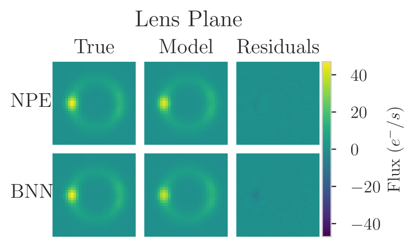
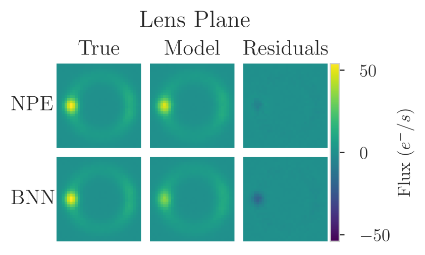
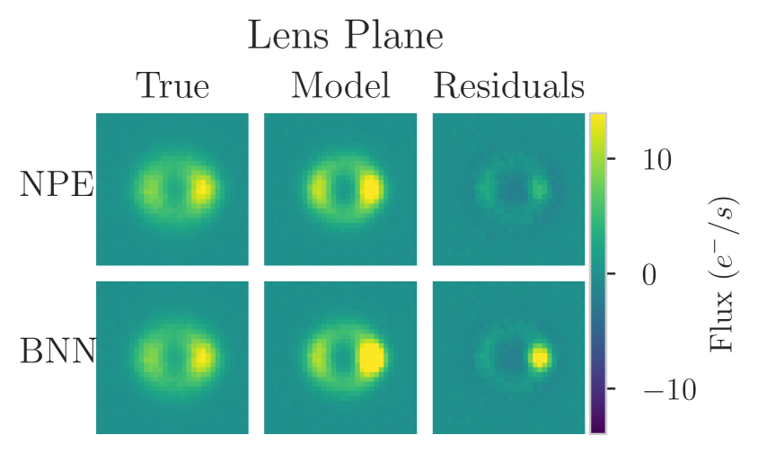
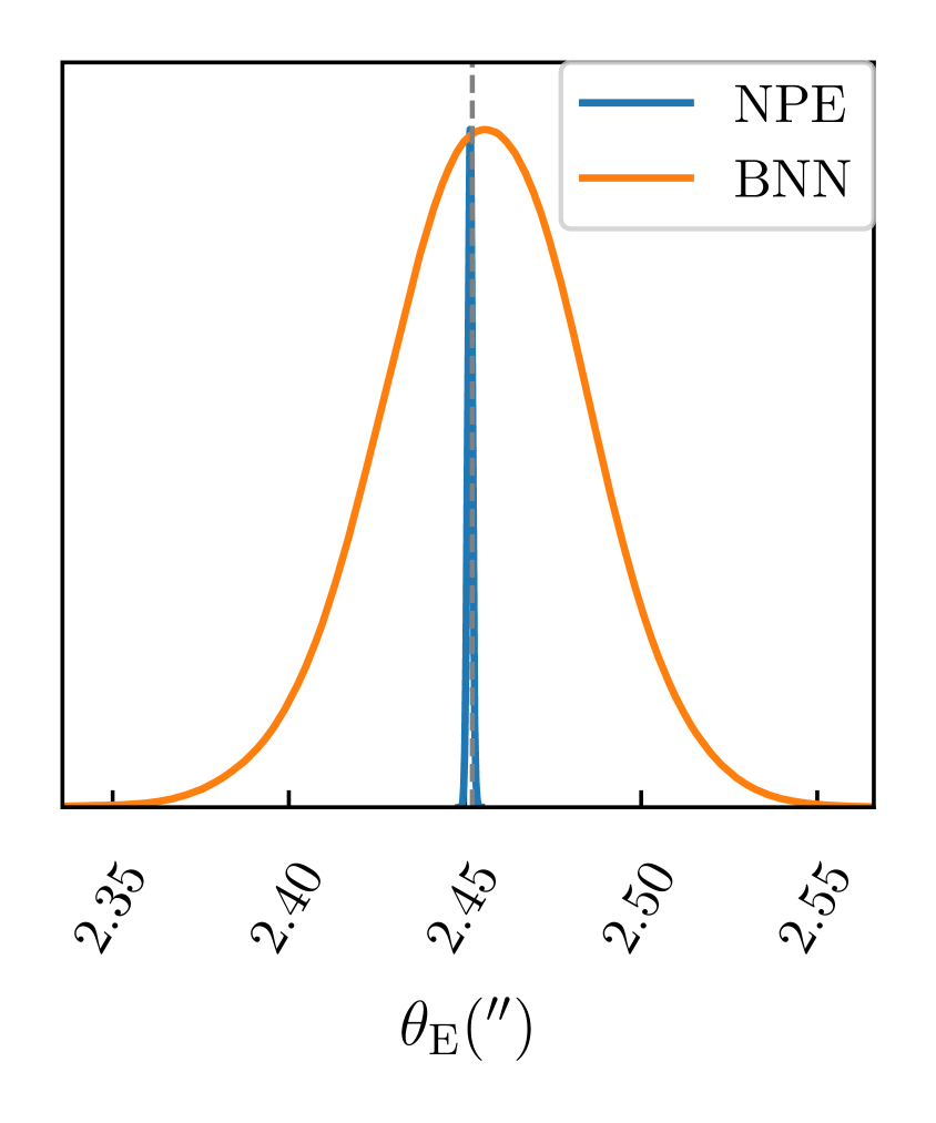
(a) Lensing system A.

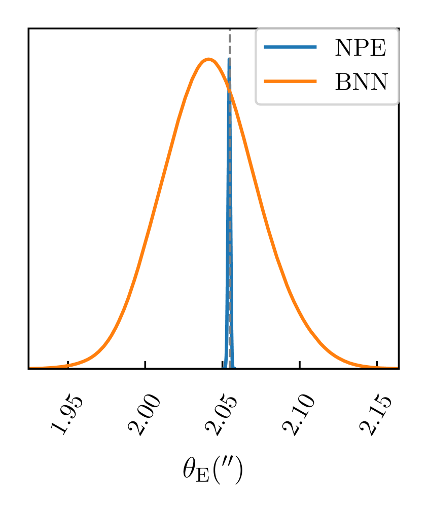
(b) Lensing system B.

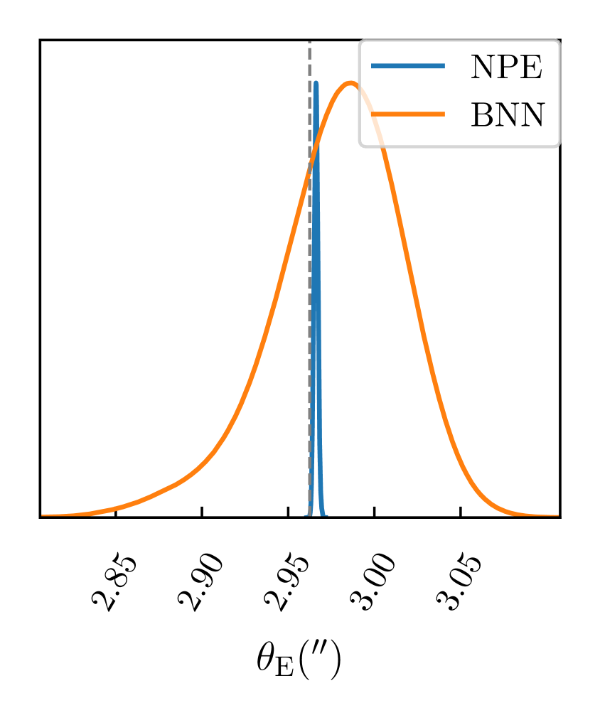
(c) Lensing system C.

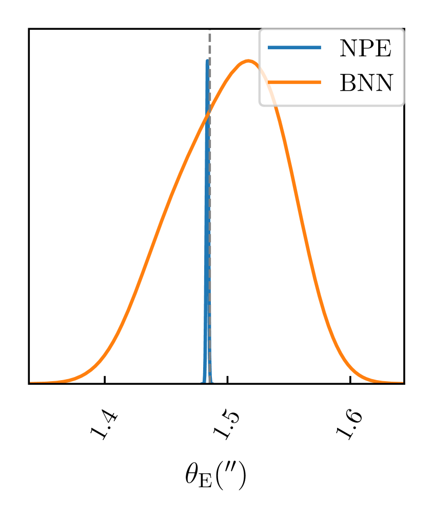
(d) Lensing system D.

Figure 21: Performance for four lensing systems (A, B, C, and D) in the 1-parameter NPE and BNN models. Top: the posterior predictive check for the lens plane image for the NPE (upper row) and the BNN (lower row) models, which includes the true image, the image predicted by each method, and the residual between the true and the predicted image for this test object. Bottom: inferred posterior of the Einstein radius $\theta_{E}$ for the NPE (blue) and BNN (orange) models.

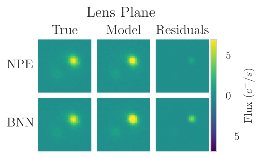
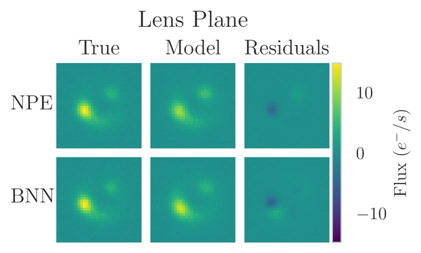
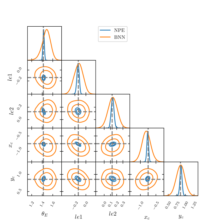
(a) Lensing system E.

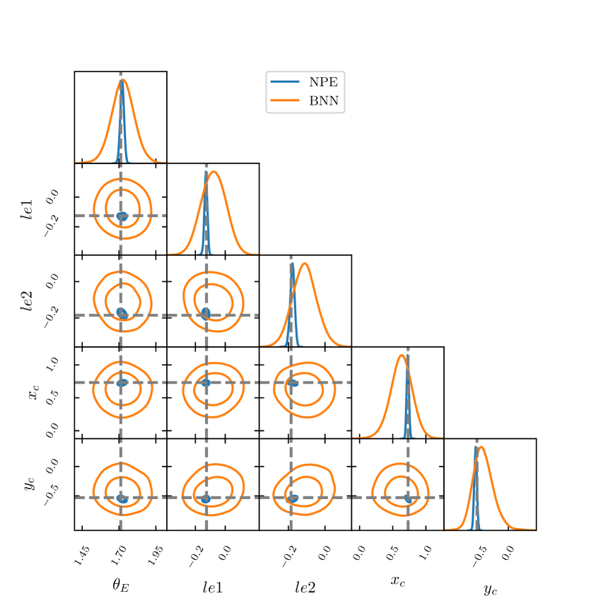
(b) Lensing system F.

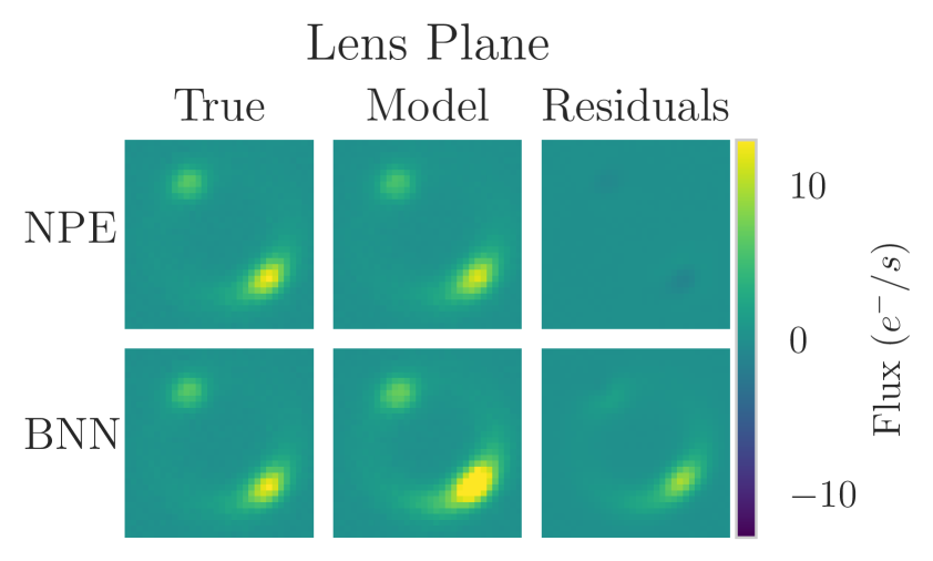
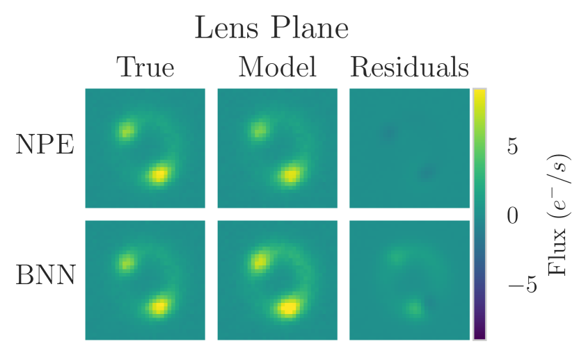
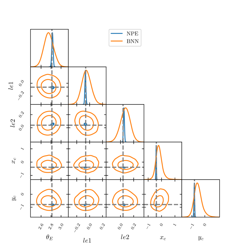
(c) Lensing system G.

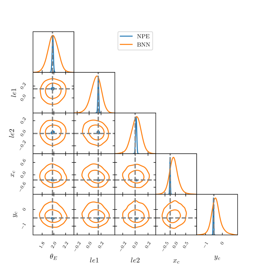
(d) Lensing system H.

Figure 22: Performance of the 5-parameter NPE and BNN models on four lensing objects drawn from the test set. Top: the posterior predictive check for the lens plane image for the NPE (upper row) and the BNN (lower row) models, which includes the true image, the image predicted by each method, and the residual between the true and the predicted image for the object. Bottom: inferred posteriors for the NPE (blue) and BNN (orange) models.

C.2 5-parameter model

Fig. 22 shows the posterior predictive image reconstruction (top) and the posterior inferences (bottom) of the NPE and BNN models for individual lensing systems (E, F, G, and H) for the 5-parameter model. The NPE model consistently provides smaller uncertainties than the BNN model for all parameters and examples. The NPE model is also consistently less biased than the BNN model for these examples; however, the NPE model is sometimes slightly biased with respect to the true posteriors. The NPE model uncertainties are about two orders of magnitude larger in the 5-parameter model than they are for the 1-parameter model.

C.3 12-parameter model

Figs. 23,  24,  25, and  26 show the posterior predictive models (top) and the posterior inferences (bottom) from the NPE and BNN models for individual lensing systems (I, J, K, and L) for the 12-parameter model. The NPE model consistently provides smaller uncertainties than the BNN model for all parameters and examples. The NPE model is also consistently less biased than the BNN model for these examples. However, the NPE model is sometimes slightly or moderately biased with respect to the true posteriors. The biases for both the NPE and BNN models are larger for more parameters in the 12-parameter model than in the 5-parameter model. The NPE model uncertainties are on the same order as or about one order of magnitude larger for the 12-parameter model compared to the 5-parameter model.

Figure 23: Performance for the 12-parameter NPE and BNN models on system I (seed 465). Top: the posterior predictive check for the lens plane image for the NPE (upper row) and the BNN (lower row) models, which includes the true image, the image predicted by each method, and the residual between the true and the predicted image for this test object. Bottom: inferred posteriors for the NPE (blue) and BNN (orange) models. The true values of parameters are indicated by dashed lines.

Figure 24: Performance for the 12-parameter NPE and BNN models on system J (seed 465). Top: the posterior predictive check for the lens plane image for the NPE (upper row) and the BNN (lower row) models, which includes the true image, the image predicted by each method, and the residual between the true and the predicted image for this test object. Bottom: inferred posteriors for the NPE (blue) and BNN (orange) models. The true values of parameters are indicated by dashed lines.

Figure 25: Performance for the 12-parameter NPE and BNN models on system K (seed 465). Top: the posterior predictive check for the lens plane image for the NPE (upper row) and the BNN (lower row) models, which includes the true image, the image predicted by each method, and the residual between the true and the predicted image for this test object. Bottom: inferred posteriors for the NPE (blue) and BNN (orange) models. The true values of parameters are indicated by dashed lines.

Figure 26: Performance for the 12-parameter NPE and BNN models on system L (seed 465). Top: the posterior predictive check for the lens plane image for the NPE (upper row) and the BNN (lower row) models, which includes the true image, the image predicted by each method, and the residual between the true and the predicted image for this test object. Bottom: inferred posteriors for the NPE (blue) and BNN (orange) models. The true values of parameters are indicated by dashed lines.

Funding

This manuscript has been supported by Fermi Research Alliance, LLC under Contract No. DE-AC02-07CH11359 with the U.S. Department of Energy (DOE), Office of Science, Office of High Energy Physics.

Author Contributions

J. Poh: Data curation, Formal analysis, Investigation, Methodology, Resources, Software, Visualization, Writing of original draft;

A. Samudre: Conceptualization, Methodology, Software, Writing (review & editing);

A. Ćiprijanović: Formal analysis, Investigation, Methodology, Software, Supervision, Writing of original draft;

G. Khullar: Methodology, Software, Writing (review & editing);

J. Frieman: Supervision, Resources, Writing (review & editing);

B. D. Nord: Conceptualization, Methodology, Resources, Supervision, Writing (review & editing)

References

- Abbott et al. [2018] T. M. C. Abbott, F. B. Abdalla, S. Allam, A. Amara, J. Annis, J. Asorey, S. Avila, O. Ballester, et al., and NOAO Data Lab. The Dark Energy Survey: Data Release 1. ApJS, 239(2):18, December 2018. doi: 10.3847/1538-4365/aae9f0.
- Abbott et al. [2021] T. M. C. Abbott, M. Adamów, M. Aguena, S. Allam, A. Amon, J. Annis, S. Avila, D. Bacon, M. Banerji, K. Bechtol, M. R. Becker, G. M. Bernstein, E. Bertin, S. Bhargava, S. L. Bridle, D. Brooks, D. L. Burke, A. Carnero Rosell, M. Carrasco Kind, J. Carretero, F. J. Castander, R. Cawthon, C. Chang, A. Choi, C. Conselice, M. Costanzi, M. Crocce, L. N. da Costa, T. M. Davis, J. De Vicente, J. DeRose, S. Desai, H. T. Diehl, J. P. Dietrich, A. Drlica-Wagner, K. Eckert, J. Elvin-Poole, S. Everett, A. E. Evrard, I. Ferrero, A. Ferté, B. Flaugher, P. Fosalba, D. Friedel, J. Frieman, J. García-Bellido, E. Gaztanaga, L. Gelman, D. W. Gerdes, T. Giannantonio, M. S. S. Gill, D. Gruen, R. A. Gruendl, J. Gschwend, G. Gutierrez, W. G. Hartley, S. R. Hinton, D. L. Hollowood, K. Honscheid, D. Huterer, D. J. James, T. Jeltema, M. D. Johnson, S. Kent, R. Kron, K. Kuehn, N. Kuropatkin, O. Lahav, T. S. Li, C. Lidman, H. Lin, N. MacCrann, M. A. G. Maia, T. A. Manning, J. D. Maloney, M. March, J. L. Marshall, P. Martini, P. Melchior, F. Menanteau, R. Miquel, R. Morgan, J. Myles, E. Neilsen, R. L. C. Ogando, A. Palmese, F. Paz-Chinchón, D. Petravick, A. Pieres, A. A. Plazas, C. Pond, M. Rodriguez-Monroy, A. K. Romer, A. Roodman, E. S. Rykoff, M. Sako, E. Sanchez, B. Santiago, V. Scarpine, S. Serrano, I. Sevilla-Noarbe, J. Allyn Smith, M. Smith, M. Soares-Santos, E. Suchyta, M. E. C. Swanson, G. Tarle, D. Thomas, C. To, P. E. Tremblay, M. A. Troxel, D. L. Tucker, D. J. Turner, T. N. Varga, A. R. Walker, R. H. Wechsler, J. Weller, W. Wester, R. D. Wilkinson, B. Yanny, Y. Zhang, R. Nikutta, M. Fitzpatrick, A. Jacques, A. Scott, K. Olsen, L. Huang, D. Herrera, S. Juneau, D. Nidever, B. A. Weaver, C. Adean, V. Correia, M. de Freitas, F. N. Freitas, C. Singulani, and G. Vila-Verde. The dark energy survey data release 2. The Astrophysical Journal Supplement Series, 255(2):20, July 2021. ISSN 1538-4365. doi: 10.3847/1538-4365/ac00b3. URL http://dx.doi.org/10.3847/1538-4365/ac00b3.
- Agnello et al. [2017] A. Agnello, H. Lin, L. Buckley-Geer, T. Treu, V. Bonvin, F. Courbin, C. Lemon, T. Morishita, A. Amara, M. W. Auger, S. Birrer, J. Chan, T. Collett, A. More, C. D. Fassnacht, J. Frieman, P. J. Marshall, R. G. McMahon, G. Meylan, S. H. Suyu, F. Castander, D. Finley, A. Howell, C. Kochanek, M. Makler, P. Martini, N. Morgan, B. Nord, F. Ostrovski, P. Schechter, D. Tucker, R. Wechsler, T. M. C. Abbott, F. B. Abdalla, S. Allam, A. Benoit-Lé vy, E. Bertin, D. Brooks, D. L. Burke, A. Carnero Rosell, M. Carrasco Kind, J. Carretero, M. Crocce, C. E. Cunha, C. B. D’Andrea, L. N. da Costa, S. Desai, J. P. Dietrich, T. F. Eifler, B. Flaugher, P. Fosalba, J. García-Bellido, E. Gaztanaga, M. S. Gill, D. A. Goldstein, D. Gruen, R. A. Gruendl, J. Gschwend, G. Gutierrez, K. Honscheid, D. J. James, K. Kuehn, N. Kuropatkin, T. S. Li, M. Lima, M. A. G. Maia, M. March, J. L. Marshall, P. Melchior, F. Menanteau, R. Miquel, R. L. C. Ogando, A. A. Plazas, A. K. Romer, E. Sanchez, R. Schindler, M. Schubnell, I. Sevilla-Noarbe, M. Smith, R. C. Smith, F. Sobreira, E. Suchyta, M. E. C. Swanson, G. Tarle, D. Thomas, and A. R. Walker. Models of the strongly lensed quasar DES j0408-5354. Monthly Notices of the Royal Astronomical Society, 472(4):4038–4050, sep 2017. doi: 10.1093/mnras/stx2242. URL https://doi.org/10.1093%2Fmnras%2Fstx2242.
- Alsing et al. [2019] Justin Alsing, Tom Charnock, Stephen Feeney, and Benjamin Wandelt. Fast likelihood-free cosmology with neural density estimators and active learning. MNRAS, 488(3):4440–4458, September 2019. doi: 10.1093/mnras/stz1960.
- Alsing et al. [2019] Justin Alsing, Tom Charnock, Stephen Feeney, and Benjamin Wandelt. Fast likelihood-free cosmology with neural density estimators and active learning. Monthly Notices of the Royal Astronomical Society, July 2019. ISSN 1365-2966. doi: 10.1093/mnras/stz1960. URL http://dx.doi.org/10.1093/mnras/stz1960.
- Anau Montel et al. [2023] Noemi Anau Montel, Adam Coogan, Camila Correa, Konstantin Karchev, and Christoph Weniger. Estimating the warm dark matter mass from strong lensing images with truncated marginal neural ratio estimation. MNRAS, 518(2):2746–2760, January 2023. doi: 10.1093/mnras/stac3215.
- Angelopoulos and Bates [2022] Anastasios N. Angelopoulos and Stephen Bates. A gentle introduction to conformal prediction and distribution-free uncertainty quantification, 2022.
- Auger et al. [2010] M. W. Auger, T. Treu, A. S. Bolton, R. Gavazzi, L. V. E. Koopmans, P. J. Marshall, L. A. Moustakas, and S. Burles. The Sloan Lens ACS Survey. X. Stellar, Dynamical, and Total Mass Correlations of Massive Early-type Galaxies. The Astrophysical Journal, Volume 724, Issue 1, pp. 511-525 (2010)., 724:511–525, jul 2010. ISSN 0004-637X. doi: 10.1088/0004-637X/724/1/511.
- Barkana [1998] Rennan Barkana. Fast calculation of a family of elliptical mass gravitational lens models. The Astrophysical Journal, Volume 502, Issue 2, pp. 531-537., 502:531–537, jan 1998. ISSN 0004-637X. doi: 10.1086/305950.
- Barnabe et al. [2011] Matteo Barnabe, Oliver Czoske, Leon V. E. Koopmans, Tommaso Treu, and Adam S. Bolton. Two-dimensional kinematics of SLACS lenses: III. Mass structure and dynamics of early-type lens galaxies beyond z ˜ 0.1. Monthly Notices of the Royal Astronomical Society, Volume 415, Issue 3, pp. 2215-2232., 415:2215–2232, feb 2011. ISSN 0035-8711. doi: 10.1111/j.1365-2966.2011.18842.x.
- Bayliss et al. [2014] Matthew B. Bayliss, Jane R. Rigby, Keren Sharon, Eva Wuyts, Michael Florian, Michael D. Gladders, Traci Johnson, and Masamune Oguri. The Physical Conditions, Metallicity and Metal Abundance Ratios in a Highly Magnified Galaxy at z = 3.6252. The Astrophysical Journal, Volume 790, Issue 2, article id. 144, 20 pp. (2014)., 790, 2014. ISSN 0004-637X. doi: 10.1088/0004-637X/790/2/144.
- Beaumont et al. [2002] Mark A Beaumont, Wenyang Zhang, and David J Balding. Approximate Bayesian Computation in Population Genetics. Genetics, 162(4):2025–2035, 12 2002. ISSN 1943-2631. doi: 10.1093/genetics/162.4.2025. URL https://doi.org/10.1093/genetics/162.4.2025.
- Bengio et al. [2014] Yoshua Bengio, Aaron Courville, and Pascal Vincent. Representation learning: A review and new perspectives, 2014.
- Birrer and Amara [2018] Simon Birrer and Adam Amara. lenstronomy: Multi-purpose gravitational lens modelling software package. Physics of the Dark Universe, 22:189–201, December 2018. doi: 10.1016/j.dark.2018.11.002.
- Birrer et al. [2017] Simon Birrer, Cyril Welschen, Adam Amara, and Alexandre Refregier. Line-of-sight effects in strong lensing: putting theory into practice. J. Cosmology Astropart. Phys, 2017(4):049, April 2017. doi: 10.1088/1475-7516/2017/04/049.
- Birrer et al. [2021] Simon Birrer, Anowar Shajib, Daniel Gilman, Aymeric Galan, Jelle Aalbers, Martin Millon, Robert Morgan, Giulia Pagano, Ji Park, Luca Teodori, Nicolas Tessore, Madison Ueland, Lyne Van de Vyvere, Sebastian Wagner-Carena, Ewoud Wempe, Lilan Yang, Xuheng Ding, Thomas Schmidt, Dominique Sluse, Ming Zhang, and Adam Amara. lenstronomy II: A gravitational lensing software ecosystem. The Journal of Open Source Software, 6(62):3283, June 2021. doi: 10.21105/joss.03283.
- Blum et al. [2013] M. G. B. Blum, M. A. Nunes, D. Prangle, and S. A. Sisson. A comparative review of dimension reduction methods in approximate bayesian computation. Statistical Science, 28(2), May 2013. ISSN 0883-4237. doi: 10.1214/12-sts406. URL http://dx.doi.org/10.1214/12-STS406.
- Bocquet and Carter [2016] Sebastian Bocquet and Faustin W. Carter. pygtc: beautiful parameter covariance plots (aka. giant triangle confusograms). The Journal of Open Source Software, 1(6), oct 2016. doi: 10.21105/joss.00046. URL http://dx.doi.org/10.21105/joss.00046.
- Bolton et al. [2008] Adam S. Bolton, Scott Burles, Léon V. E. Koopmans, Tommaso Treu, Raphaël Gavazzi, Leonidas A. Moustakas, Randall Wayth, and David J. Schlegel. The Sloan Lens ACS Survey. V. The Full ACS Strong-Lens Sample. ApJ, 682(2):964–984, August 2008. doi: 10.1086/589327.
- Bom et al. [2019] Clecio Bom, Jason Poh, Brian Nord, Manuel Blanco-Valentin, and Luciana Dias. Deep learning in wide-field surveys: Fast analysis of strong lenses in ground-based cosmic experiments, 2019.
- Brehmer et al. [2018a] Johann Brehmer, Kyle Cranmer, Gilles Louppe, and Juan Pavez. Constraining effective field theories with machine learning. Physical Review Letters, 121(11), sep 2018a. doi: 10.1103/physrevlett.121.111801. URL https://doi.org/10.1103%2Fphysrevlett.121.111801.
- Brehmer et al. [2018b] Johann Brehmer, Kyle Cranmer, Gilles Louppe, and Juan Pavez. A guide to constraining effective field theories with machine learning, 2018b.
- Brehmer et al. [2019] Johann Brehmer, Siddharth Mishra-Sharma, Joeri Hermans, Gilles Louppe, and Kyle Cranmer. Mining for Dark Matter Substructure: Inferring Subhalo Population Properties from Strong Lenses with Machine Learning. ApJ, 886(1):49, November 2019. doi: 10.3847/1538-4357/ab4c41.
- Brehmer et al. [2019] Johann Brehmer, Siddharth Mishra-Sharma, Joeri Hermans, Gilles Louppe, and Kyle Cranmer. Mining for dark matter substructure: Inferring subhalo population properties from strong lenses with machine learning. The Astrophysical Journal, 886(1):49, nov 2019. doi: 10.3847/1538-4357/ab4c41. URL https://doi.org/10.3847%2F1538-4357%2Fab4c41.
- Butter et al. [2022] Anja Butter, Thorben Finke, Felicitas Keil, Michael Krämer, and Silvia Manconi. Classification of Fermi-LAT blazars with Bayesian neural networks. J. Cosmology Astropart. Phys, 2022(4):023, April 2022. doi: 10.1088/1475-7516/2022/04/023.
- Cameron and Pettitt [2012] E. Cameron and A. N. Pettitt. Approximate Bayesian Computation for astronomical model analysis: a case study in galaxy demographics and morphological transformation at high redshift. MNRAS, 425(1):44–65, September 2012. doi: 10.1111/j.1365-2966.2012.21371.x.
- Charnock et al. [2018] Tom Charnock, Guilhem Lavaux, and Benjamin D. Wandelt. Automatic physical inference with information maximizing neural networks. Physical Review D, 97(8), April 2018. ISSN 2470-0029. doi: 10.1103/physrevd.97.083004. URL http://dx.doi.org/10.1103/PhysRevD.97.083004.
- Chen et al. [2019] Yun Chen, Ran Li, Yiping Shu, and Xiaoyue Cao. Assessing the effect of lens mass model in cosmological application with updated galaxy-scale strong gravitational lensing sample. Monthly Notices of the Royal Astronomical Society, 488(3):3745–3758, July 2019. ISSN 1365-2966. doi: 10.1093/mnras/stz1902. URL http://dx.doi.org/10.1093/mnras/stz1902.
- Christensen et al. [2012] Lise Christensen, Peter Laursen, Johan Richard, Jens Hjorth, Bo Milvang-Jensen, Miroslava Dessauges-Zavadsky, Marceau Limousin, Claudio Grillo, and Harald Ebeling. Gravitationally Lensed Galaxies at 2. Monthly Notices of the Royal Astronomical Society, Volume 427, Issue 3, pp. 1973-1982., 427:1973–1982, sep 2012. ISSN 0035-8711. doi: 10.1111/j.1365-2966.2012.22007.x.
- Ciotti and Bertin [1999] L. Ciotti and G. Bertin. Analytical properties of the R1/m law. A&A, 352:447–451, December 1999.
- Collett et al. [2012] T. E. Collett, M. W. Auger, V. Belokurov, P. J. Marshall, and A. C. Hall. Constraining the dark energy equation of state with double-source plane strong lenses. Monthly Notices of the Royal Astronomical Society, Volume 424, Issue 4, pp. 2864-2875., 424:2864–2875, 2012. ISSN 0035-8711. doi: 10.1111/J.1365-2966.2012.21424.X.
- Collett [2015] Thomas E. Collett. The Population of Galaxy-Galaxy Strong Lenses in Forthcoming Optical Imaging Surveys. ApJ, 811(1):20, September 2015. doi: 10.1088/0004-637X/811/1/20.
- Collett and Auger [2014] Thomas E. Collett and Matthew W. Auger. Cosmological constraints from the double source plane lens SDSSJ0946+1006. Monthly Notices of the Royal Astronomical Society, Volume 443, Issue 2, p.969-976, 443:969–976, 2014. ISSN 0035-8711. doi: 10.1093/MNRAS/STU1190.
- Coogan et al. [2022] Adam Coogan, Noemi Anau Montel, Konstantin Karchev, Meiert W. Grootes, Francesco Nattino, and Christoph Weniger. One never walks alone: the effect of the perturber population on subhalo measurements in strong gravitational lenses. arXiv e-prints, art. arXiv:2209.09918, September 2022.
- Cook et al. [2006] Samantha Cook, Andrew Gelman, and Donald Rubin. Validation of software for bayesian models using posterior quantiles. Journal of Computational and Graphical Statistics - J COMPUT GRAPH STAT, 15, 09 2006. doi: 10.1198/106186006X136976.
- Cranmer et al. [2019] Kyle Cranmer, Johann Brehmer, and Gilles Louppe. The frontier of simulation-based inference. arXiv e-prints, art. arXiv:1911.01429, November 2019.
- Dark Energy Survey Collaboration et al. [2016] Dark Energy Survey Collaboration, T. Abbott, F. B. Abdalla, J. Aleksić, S. Allam, A. Amara, D. Bacon, E. Balbinot, M. Banerji, K. Bechtol, A. Benoit-Lévy, and et al. The Dark Energy Survey: more than dark energy - an overview. MNRAS, 460(2):1270–1299, August 2016. doi: 10.1093/mnras/stw641.
- Deistler et al. [2022] Michael Deistler, Pedro J Goncalves, and Jakob H Macke. Truncated proposals for scalable and hassle-free simulation-based inference, 2022.
- Dessauges-Zavadsky et al. [2009] M. Dessauges-Zavadsky, S. D’Odorico, D. Schaerer, A. Modigliani, C. Tapken, and J. Vernet. Rest-frame ultraviolet spectrum of the gravitationally lensed galaxy ‘the 8 o’clock arc’: stellar and interstellar medium properties. Astronomy and Astrophysics, Volume 510, id.A26, 510, dec 2009. ISSN 0004-6361. doi: 10.1051/0004-6361/200913337.
- Durkan et al. [2020] Conor Durkan, Iain Murray, and George Papamakarios. On contrastive learning for likelihood-free inference, 2020.
- Escamilla-Rivera et al. [2022] Celia Escamilla-Rivera, Maryi Carvajal, Cristian Zamora, and Martin Hendry. Neural networks and standard cosmography with newly calibrated high redshift GRB observations. J. Cosmology Astropart. Phys, 2022(4):016, April 2022. doi: 10.1088/1475-7516/2022/04/016.
- Finkelstein et al. [2009] Steven L. Finkelstein, Casey Papovich, Gregory Rudnick, Eiichi Egami, Emeric Le Floc’h, Marcia J. Rieke, Jane Rigby, and Christopher N. A. Willmer. Turning Back the Clock: Inferring the History of the Eight O’clock Arc. The Astrophysical Journal, Volume 700, Issue 1, pp. 376-386 (2009)., 700:376–386, may 2009. ISSN 0004-637X. doi: 10.1088/0004-637X/700/1/376.
- Foreman-Mackey [2016] Daniel Foreman-Mackey. corner.py: Scatterplot matrices in python. The Journal of Open Source Software, 1(2):24, jun 2016. doi: 10.21105/joss.00024. URL https://doi.org/10.21105/joss.00024.
- Gabry et al. [2019] Jonah Gabry, Daniel Simpson, Aki Vehtari, Michael Betancourt, and Andrew Gelman. Visualization in Bayesian Workflow. Journal of the Royal Statistical Society Series A: Statistics in Society, 182(2):389–402, 01 2019. ISSN 0964-1998. doi: 10.1111/rssa.12378. URL https://doi.org/10.1111/rssa.12378.
- Gavazzi et al. [2008] Raphael Gavazzi, Tommaso Treu, Leon V. E. Koopmans, Adam S. Bolton, Leonidas A. Moustakas, Scott Burles, and Philip J. Marshall. The Sloan Lens ACS Survey. VI: Discovery and analysis of a double Einstein ring. The Astrophysical Journal, Volume 677, Issue 2, article id. 1046-1059, pp. (2008)., 677, jan 2008. ISSN 0004-637X. doi: 10.1086/529541.
- Gerardi et al. [2021] Francesca Gerardi, Stephen M. Feeney, and Justin Alsing. Unbiased likelihood-free inference of the Hubble constant from light standard sirens. Phys. Rev. D, 104(8):083531, October 2021. doi: 10.1103/PhysRevD.104.083531.
- Germain et al. [2015] Mathieu Germain, Karol Gregor, Iain Murray, and Hugo Larochelle. Made: Masked autoencoder for distribution estimation. In Francis Bach and David Blei, editors, Proceedings of the 32nd International Conference on Machine Learning, volume 37 of Proceedings of Machine Learning Research, pages 881–889, Lille, France, 07–09 Jul 2015. PMLR. URL https://proceedings.mlr.press/v37/germain15.html.
- Goncalves et al. [2020] Pedro Goncalves, Jan-Matthis Lueckmann, Michael Deistler, Marcel Nonnenmacher, Kaan Öcal, Giacomo Bassetto, Chaitanya Chintaluri, William Podlaski, Sara Haddad, Tim Vogels, David Greenberg, and Jakob Macke. Training deep neural density estimators to identify mechanistic models of neural dynamics. eLife, 9, 09 2020. doi: 10.7554/eLife.56261.
- Graves [2011] Alex Graves. Practical variational inference for neural networks. In J. Shawe-Taylor, R. Zemel, P. Bartlett, F. Pereira, and K.Q. Weinberger, editors, Advances in Neural Information Processing Systems, volume 24. Curran Associates, Inc., 2011. URL https://proceedings.neurips.cc/paper/2011/file/7eb3c8be3d411e8ebfab08eba5f49632-Paper.pdf.
- Greenberg et al. [2019] David Greenberg, Marcel Nonnenmacher, and Jakob Macke. Automatic posterior transformation for likelihood-free inference. In International Conference on Machine Learning, pages 2404–2414. PMLR, 2019.
- Guo et al. [2017] Chuan Guo, Geoff Pleiss, Yu Sun, and Kilian Q. Weinberger. On calibration of modern neural networks, 2017.
- Hainline et al. [2009] Kevin N. Hainline, Alice E. Shapley, Katherine A. Kornei, Max Pettini, Elizabeth Buckley-Geer, Sahar S. Allam, and Douglas L. Tucker. Rest-Frame Optical Spectra of Three Strongly Lensed Galaxies at z˜2. arxiv, jun 2009. doi: 10.1088/0004-637X/701/1/52.
- Heinrich et al. [2024] Lukas Heinrich, Siddharth Mishra-Sharma, Chris Pollard, and Philipp Windischhofer. Hierarchical neural simulation-based inference over event ensembles, 2024. URL https://arxiv.org/abs/2306.12584.
- Hermans et al. [2022] Joeri Hermans, Arnaud Delaunoy, François Rozet, Antoine Wehenkel, Volodimir Begy, and Gilles Louppe. A trust crisis in simulation-based inference? your posterior approximations can be unfaithful, 2022.
- Hezaveh et al. [2017] Yashar D. Hezaveh, Laurence Perreault Levasseur, and Philip J. Marshall. Fast automated analysis of strong gravitational lenses with convolutional neural networks. Nature, 548(7669):555–557, aug 2017. doi: 10.1038/nature23463. URL https://doi.org/10.1038%2Fnature23463.
- Hortúa et al. [2020] Hé ctor J. Hortúa, Riccardo Volpi, Dimitri Marinelli, and Luigi Malagò. Parameter estimation for the cosmic microwave background with bayesian neural networks. Physical Review D, 102(10), nov 2020. doi: 10.1103/physrevd.102.103509. URL https://doi.org/10.1103%2Fphysrevd.102.103509.
- Huang et al. [2022] Kuan-Wei Huang, Geoff Chih-Fan Chen, Po-Wen Chang, Sheng-Chieh Lin, Chia-Jung Hsu, Vishal Thengane, and Joshua Yao-Yu Lin. Strong gravitational lensing parameter estimation with vision transformer. arXiv preprint arXiv:2210.04143, 2022.
- Huppenkothen and Bachetti [2021] D. Huppenkothen and M. Bachetti. Accurate X-ray Timing in the Presence of Systematic Biases With Simulation-Based Inference. arXiv e-prints, art. arXiv:2104.03278, April 2021.
- Ivezić et al. [2019] Željko Ivezić, Steven M. Kahn, J. Anthony Tyson, Bob Abel, Emily Acosta, Robyn Allsman, David Alonso, Yusra AlSayyad, and et al. LSST: From science drivers to reference design and anticipated data products. ApJ, 873(2):111, March 2019. doi: 10.3847/1538-4357/ab042c.
- Iwata et al. [2008] I. Iwata, A. K. Inoue, Y. Matsuda, H. Furusawa, T. Hayashino, K. Kousai, M. Akiyama, T. Yamada, D. Burgarella, and J. M. Deharveng. Detections of Lyman Continuum from Star-forming Galaxies at z˜3 Through Subaru/Suprime-Cam Narrow-band Imaging. The Astrophysical Journal, Volume 692, Issue 2, pp. 1287-1293 (2009)., 692:1287–1293, may 2008. ISSN 0004-637X. doi: 10.1088/0004-637X/692/2/1287.
- Jacobs et al. [2017] C. Jacobs, K. Glazebrook, T. Collett, A. More, and C. McCarthy. Finding strong lenses in cfhtls using convolutional neural networks. Monthly Notices of the Royal Astronomical Society, 471(1):167–181, June 2017. ISSN 1365-2966. doi: 10.1093/mnras/stx1492. URL http://dx.doi.org/10.1093/mnras/stx1492.
- Jacobs et al. [2019] C. Jacobs, T. Collett, K. Glazebrook, E. Buckley-Geer, H. T. Diehl, H. Lin, C. McCarthy, A. K. Qin, C. Odden, M. Caso Escudero, P. Dial, V. J. Yung, S. Gaitsch, A. Pellico, K. A. Lindgren, T. M. C. Abbott, J. Annis, S. Avila, D. Brooks, D. L. Burke, A. Carnero Rosell, M. Carrasco Kind, J. Carretero, L. N. da Costa, J. De Vicente, P. Fosalba, J. Frieman, J. García-Bellido, E. Gaztanaga, D. A. Goldstein, D. Gruen, R. A. Gruendl, J. Gschwend, D. L. Hollowood, K. Honscheid, B. Hoyle, D. J. James, E. Krause, N. Kuropatkin, O. Lahav, M. Lima, M. A. G. Maia, J. L. Marshall, R. Miquel, A. A. Plazas, A. Roodman, E. Sanchez, V. Scarpine, S. Serrano, I. Sevilla-Noarbe, M. Smith, F. Sobreira, E. Suchyta, M. E. C. Swanson, G. Tarle, V. Vikram, A. R. Walker, and Y. Zhang. An extended catalog of galaxy–galaxy strong gravitational lenses discovered in des using convolutional neural networks. The Astrophysical Journal Supplement Series, 243(1):17, July 2019. ISSN 1538-4365. doi: 10.3847/1538-4365/ab26b6. URL http://dx.doi.org/10.3847/1538-4365/ab26b6.
- James et al. [2013] Bethan L. James, Max Pettini, Lise Christensen, Matthew W. Auger, George D. Becker, Lindsay J. King, Anna M. Quider, Alice E. Shapley, and Charles C. Steidel. Testing metallicity indicators at z˜1.4 with the gravitationally lensed galaxy CASSOWARY 20. Monthly Notices of the Royal Astronomical Society, Volume 440, Issue 2, p.1794-1809, 440:1794–1809, nov 2013. ISSN 0035-8711. doi: 10.1093/mnras/stu287.
- Jarugula et al. [2024] Sreevani Jarugula, Brian D. Nord, Abhijith Gandrakota, and Alexandra Ciprijanovic. Population-level Dark Energy Constraints from Strong Lensing using Neural Ratio Estimation. Accepted to ICML AI for Science Workshop, 2024.
- Jee et al. [2016] I. Jee, E. Komatsu, S.H. Suyu, and D. Huterer. Time-delay cosmography: increased leverage with angular diameter distances. Journal of Cosmology and Astroparticle Physics, 2016(04):031–031, April 2016. ISSN 1475-7516. doi: 10.1088/1475-7516/2016/04/031. URL http://dx.doi.org/10.1088/1475-7516/2016/04/031.
- Jee et al. [2019] Inh Jee, Sherry H. Suyu, Eiichiro Komatsu, Christopher D. Fassnacht, Stefan Hilbert, and Léon V. E. Koopmans. A measurement of the hubble constant from angular diameter distances to two gravitational lenses. Science, 365(6458):1134–1138, September 2019. ISSN 1095-9203. doi: 10.1126/science.aat7371. URL http://dx.doi.org/10.1126/science.aat7371.
- Jennings and Madigan [2017] E. Jennings and M. Madigan. astroabc: An approximate bayesian computation sequential monte carlo sampler for cosmological parameter estimation. Astronomy and Computing, 19:16–22, April 2017. ISSN 2213-1337. doi: 10.1016/j.ascom.2017.01.001. URL http://dx.doi.org/10.1016/j.ascom.2017.01.001.
- Jones et al. [2013] Tucker Jones, Richard S. Ellis, Matthew A. Schenker, and Daniel P. Stark. Keck Spectroscopy of Gravitationally Lensed z=4 Galaxies: Improved Constraints on the Escape Fraction of Ionizing Photons. The Astrophysical Journal, Volume 779, Issue 1, article id. 52, 8 pp. (2013)., 779, apr 2013. ISSN 0004-637X. doi: 10.1088/0004-637X/779/1/52.
- Jospin et al. [2022] Laurent Valentin Jospin, Hamid Laga, Farid Boussaid, Wray Buntine, and Mohammed Bennamoun. Hands-on bayesian neural networks—a tutorial for deep learning users. IEEE Computational Intelligence Magazine, 17(2):29–48, 2022. doi: 10.1109/MCI.2022.3155327.
- Kassiola and Kovner [1993] Aggeliki Kassiola and Israel Kovner. Elliptic Mass Distributions versus Elliptic Potentials in Gravitational Lenses. The Astrophysical Journal, 417:450, nov 1993. ISSN 0004-637X. doi: 10.1086/173325.
- Keeton et al. [1997] C. R. Keeton, C. S. Kochanek, and U. Seljak. Shear and ellipticity in gravitational lenses. The Astrophysical Journal, 482(2):604–620, jun 1997. doi: 10.1086/304172. URL https://doi.org/10.1086%2F304172.
- Kingma and Ba [2017] Diederik P. Kingma and Jimmy Ba. Adam: A method for stochastic optimization, 2017.
- Knabel et al. [2023] Shawn Knabel, B W Holwerda, J Nightingale, T Treu, M Bilicki, S Brough, S Driver, L Finnerty, L Haberzettl, S Hegde, A M Hopkins, K Kuijken, J Liske, A K Pimblett, R C Steele, and A H Wright. Modelling strong lenses from wide-field ground-based observations in KiDS and GAMA. Monthly Notices of the Royal Astronomical Society, 520(1):804–827, jan 2023. doi: 10.1093/mnras/stad133. URL https://doi.org/10.1093%2Fmnras%2Fstad133.
- Kneib et al. [2011] Jean-Paul Kneib, Henri Bonnet, Ghyslain Golse, David Sand, Eric Jullo, and Phil Marshall. LENSTOOL: A Gravitational Lensing Software for Modeling Mass Distribution of Galaxies and Clusters (strong and weak regime). Astrophysics Source Code Library, record ascl:1102.004, February 2011.
- Kormann et al. [1994] R. Kormann, P. Schneider, and M. Bartelmann. Astronomy and astrophysics. Astronomy and Astrophysics (ISSN 0004-6361), vol. 284, no. 1, p. 285-299, 284(1):285–299, 1994.
- Kull et al. [2017] Meelis Kull, Telmo Silva Filho, and Peter Flach. Beta calibration: a well-founded and easily implemented improvement on logistic calibration for binary classifiers. In Aarti Singh and Jerry Zhu, editors, Proceedings of the 20th International Conference on Artificial Intelligence and Statistics, volume 54 of Proceedings of Machine Learning Research, pages 623–631. PMLR, 20–22 Apr 2017. URL https://proceedings.mlr.press/v54/kull17a.html.
- Kullback and Leibler [1951] Solomon Kullback and Richard A Leibler. On information and sufficiency. The annals of mathematical statistics, 22(1):79–86, 1951.
- Lefor et al. [2013] Alan T. Lefor, Toshifumi Futamase, and Mohammad Akhlaghi. A systematic review of strong gravitational lens modeling software. New Astronomy Reviews, 57(1–2):1–13, July 2013. ISSN 1387-6473. doi: 10.1016/j.newar.2013.05.001. URL http://dx.doi.org/10.1016/j.newar.2013.05.001.
- Legin et al. [2021] Ronan Legin, Yashar Hezaveh, Laurence Perreault Levasseur, and Benjamin Wandelt. Simulation-Based Inference of Strong Gravitational Lensing Parameters. arXiv e-prints, art. arXiv:2112.05278, December 2021.
- Legin et al. [2022] Ronan Legin, Yashar Hezaveh, Laurence Perreault-Levasseur, and Benjamin Wandelt. A framework for obtaining accurate posteriors of strong gravitational lensing parameters with flexible priors and implicit likelihoods using density estimation. arXiv preprint arXiv:2212.00044, 2022.
- Legin et al. [2023] Ronan Legin, Yashar Hezaveh, Laurence Perreault-Levasseur, and Benjamin Wandelt. A Framework for Obtaining Accurate Posteriors of Strong Gravitational Lensing Parameters with Flexible Priors and Implicit Likelihoods Using Density Estimation. ApJ, 943(1):4, January 2023. doi: 10.3847/1538-4357/aca7c2.
- Lemon [2017] Cameron Lemon. Gravitationally lensed quasar database, 2017. URL https://research.ast.cam.ac.uk/lensedquasars/.
- Levasseur et al. [2017] Laurence Perreault Levasseur, Yashar D Hezaveh, and Risa H Wechsler. Uncertainties in parameters estimated with neural networks: Application to strong gravitational lensing. The Astrophysical Journal Letters, 850(1):L7, 2017.
- Lewis [2019] Antony Lewis. Getdist: a python package for analysing monte carlo samples, 2019.
- Li et al. [2022] Zewen Li, Fan Liu, Wenjie Yang, Shouheng Peng, and Jun Zhou. A survey of convolutional neural networks: Analysis, applications, and prospects. IEEE Transactions on Neural Networks and Learning Systems, 33(12):6999–7019, 2022. doi: 10.1109/TNNLS.2021.3084827.
- Lin et al. [2021] Zhen Lin, Shubhendu Trivedi, and Jimeng Sun. Locally valid and discriminative prediction intervals for deep learning models, 2021.
- Lueckmann et al. [2018] Jan-Matthis Lueckmann, Giacomo Bassetto, Theofanis Karaletsos, and Jakob H. Macke. Likelihood-free inference with emulator networks. arXiv e-prints, art. arXiv:1805.09294, May 2018. doi: 10.48550/arXiv.1805.09294.
- Lueckmann et al. [2021] Jan-Matthis Lueckmann, Jan Boelts, David S. Greenberg, Pedro J. Gonçalves, and Jakob H. Macke. Benchmarking simulation-based inference, 2021.
- Mahler et al. [2023] Guillaume Mahler, Mathilde Jauzac, Johan Richard, Benjamin Beauchesne, Harald Ebeling, David Lagattuta, Priyamvada Natarajan, Keren Sharon, Hakim Atek, Adélaïde Claeyssens, Benjamin Clément, Dominique Eckert, Alastair Edge, Jean-Paul Kneib, and Anna Niemiec. Precision modeling of jwst’s first cluster lens smacsj0723.3-7327, 2023.
- Mancini et al. [2022] A. Spurio Mancini, M. M. Docherty, M. A. Price, and J. D. McEwen. Bayesian model comparison for simulation-based inference, 2022.
- Modrák et al. [2023] Martin Modrák, Angie H. Moon, Shinyoung Kim, Paul Bürkner, Niko Huurre, Kateřina Faltejsková, Andrew Gelman, and Aki Vehtari. Simulation-based calibration checking for bayesian computation: The choice of test quantities shapes sensitivity. Bayesian Analysis, Advance publication, 2023. doi: 10.1214/23-BA1404.
- Morgan et al. [2021] Robert Morgan, Brian Nord, Simon Birrer, Joshua Lin, and Jason Poh. deeplenstronomy: A dataset simulation package for strong gravitational lensing. The Journal of Open Source Software, 6(58):2854, February 2021. doi: 10.21105/joss.02854.
- Moustakas [2012] Leonidas Moustakas. The Master Lens Database and The Orphan Lenses Project. HST Proposal ID 12833. Cycle 20, October 2012.
- Narayan and Bartelmann [1996] Ramesh Narayan and Matthias Bartelmann. Lectures on Gravitational Lensing. eprint arXiv:astro-ph/9606001, jun 1996.
- Neal [1996] R. M Neal. Bayesian Learning for Neural Networks, volume 118. Springer Science & Business Media, 1996. ISBN 978-0-387-94724-2.
- Newman et al. [2012a] Andrew B. Newman, Tommaso Treu, Richard S. Ellis, and David J. Sand. The Density Profiles of Massive, Relaxed Galaxy Clusters. II. Separating Luminous and Dark Matter in Cluster Cores. The Astrophysical Journal, Volume 765, Issue 1, article id. 25, 12 pp. (2013)., 765, sep 2012a. ISSN 0004-637X. doi: 10.1088/0004-637X/765/1/25.
- Newman et al. [2012b] Andrew B. Newman, Tommaso Treu, Richard S. Ellis, David J. Sand, Carlo Nipoti, Johan Richard, and Eric Jullo. The Density Profiles of Massive, Relaxed Galaxy Clusters. I. The Total Density Over Three Decades in Radius. The Astrophysical Journal, Volume 765, Issue 1, article id. 24, 35 pp. (2013)., 765, sep 2012b. ISSN 0004-637X. doi: 10.1088/0004-637X/765/1/24.
- Newman et al. [2015] Andrew B. Newman, Richard S. Ellis, and Tommaso Treu. Luminous and Dark Matter Profiles from Galaxies to Clusters: Bridging the Gap with Group-scale Lenses. The Astrophysical Journal, Volume 814, Issue 1, article id. 26, 28 pp. (2015)., 814, 2015. ISSN 0004-637X. doi: 10.1088/0004-637X/814/1/26.
- Nightingale [2016] James J.N. Nightingale. AutoLens: automated modeling of a strong lens’s light, mass and source. PhD thesis, School of Physics and Astronomy, Nottingham University, University Park, Nottingham, NG7 2RD, UK, dec 2016. URL http://eprints.nottingham.ac.uk/38507/.
- Nord et al. [2016] B. Nord, E. Buckley-Geer, H. Lin, H. T. Diehl, J. Helsby, N. Kuropatkin, A. Amara, T. Collett, S. Allam, G. B. Caminha, C. De Bom, S. Desai, H. Dúmet-Montoya, M. Elidaiana da S. Pereira, D. A. Finley, B. Flaugher, C. Furlanetto, H. Gaitsch, M. Gill, K. W. Merritt, A. More, D. Tucker, A. Saro, E. S. Rykoff, E. Rozo, S. Birrer, F. B. Abdalla, A. Agnello, M. Auger, R. J. Brunner, M. Carrasco Kind, F. J. Castander, C. E. Cunha, L. N. da Costa, R. J. Foley, D. W. Gerdes, K. Glazebrook, J. Gschwend, W. Hartley, R. Kessler, D. Lagattuta, G. Lewis, M. A. G. Maia, M. Makler, F. Menanteau, A. Niernberg, D. Scolnic, J. D. Vieira, R. Gramillano, T. M. C. Abbott, M. Banerji, A. Benoit-Lévy, D. Brooks, D. L. Burke, D. Capozzi, A. Carnero Rosell, J. Carretero, C. B. D’Andrea, J. P. Dietrich, P. Doel, A. E. Evrard, J. Frieman, E. Gaztanaga, D. Gruen, K. Honscheid, D. J. James, K. Kuehn, T. S. Li, M. Lima, J. L. Marshall, P. Martini, P. Melchior, R. Miquel, E. Neilsen, R. C. Nichol, R. Ogando, A. A. Plazas, A. K. Romer, M. Sako, E. Sanchez, V. Scarpine, M. Schubnell, I. Sevilla-Noarbe, R. C. Smith, M. Soares-Santos, F. Sobreira, E. Suchyta, M. E. C. Swanson, G. Tarle, J. Thaler, A. R. Walker, W. Wester, Y. Zhang, and DES Collaboration. Observation and Confirmation of Six Strong-lensing Systems in the Dark Energy Survey Science Verification Data. The Astrophysical Journal, Volume 827, Issue 1, article id. 51, 16 pp. (2016)., 827, 2016. ISSN 0004-637X. doi: 10.3847/0004-637X/827/1/51.
- Oguri and Marshall [2010] Masamune Oguri and Philip J. Marshall. Gravitationally lensed quasars and supernovae in future wide-field optical imaging surveys. Monthly Notices of the Royal Astronomical Society, Volume 405, Issue 4, pp. 2579-2593., 405:2579–2593, 2010. ISSN 0035-8711. doi: 10.1111/J.1365-2966.2010.16639.X.
- Papamakarios and Murray [2018] George Papamakarios and Iain Murray. Fast -free inference of simulation models with bayesian conditional density estimation, 2018.
- Papamakarios et al. [2017] George Papamakarios, Theo Pavlakou, and Iain Murray. Masked autoregressive flow for density estimation. arXiv preprint arXiv:1705.07057, 2017.
- Papamakarios et al. [2021] George Papamakarios, Eric Nalisnick, Danilo Jimenez Rezende, Shakir Mohamed, and Balaji Lakshminarayanan. Normalizing flows for probabilistic modeling and inference. Journal of Machine Learning Research, 22(57):1–64, 2021. URL http://jmlr.org/papers/v22/19-1028.html.
- Park et al. [2021] Ji Won Park, Sebastian Wagner-Carena, Simon Birrer, Philip J Marshall, Joshua Yao-Yu Lin, Aaron Roodman, LSST Dark Energy Science Collaboration, et al. Large-scale gravitational lens modeling with bayesian neural networks for accurate and precise inference of the hubble constant. The Astrophysical Journal, 910(1):39, 2021.
- Pearson et al. [2021] James Pearson, Jacob Maresca, Nan Li, and Simon Dye. Strong lens modelling: comparing and combining bayesian neural networks and parametric profile fitting. Monthly Notices of the Royal Astronomical Society, 505(3):4362–4382, 2021.
- Picard [2021] David Picard. Torch.manual_seed(3407) is all you need: On the influence of random seeds in deep learning architectures for computer vision. arXiv e-prints, art. arXiv:2109.08203, September 2021. doi: 10.48550/arXiv.2109.08203.
- Prangle [2015] Dennis Prangle. Summary statistics in approximate bayesian computation, 2015.
- Quider et al. [2009] Anna M. Quider, Max Pettini, Alice E. Shapley, and Charles C. Steidel. The Ultraviolet Spectrum of the Gravitationally Lensed Galaxy ‘The Cosmic Horseshoe’: A Close-up of a Star-forming Galaxy at z = 2. Monthly Notices of the Royal Astronomical Society, Volume 398, Issue 3, pp. 1263-1278., 398:1263–1278, jun 2009. ISSN 0035-8711. doi: 10.1111/j.1365-2966.2009.15234.x.
- Racca et al. [2016] Giuseppe D. Racca, René Laureijs, Luca Stagnaro, Jean-Christophe Salvignol, José Lorenzo Alvarez, Gonzalo Saavedra Criado, Luis Gaspar Venancio, Alex Short, Paolo Strada, Tobias Bönke, Cyril Colombo, Adriano Calvi, Elena Maiorano, Osvaldo Piersanti, Sylvain Prezelus, Pierluigi Rosato, Jacques Pinel, Hans Rozemeijer, Valentina Lesna, Paolo Musi, Marco Sias, Alberto Anselmi, Vincent Cazaubiel, Ludovic Vaillon, Yannick Mellier, Jérôme Amiaux, Michel Berthé, Marc Sauvage, Ruyman Azzollini, Mark Cropper, Sabrina Pottinger, Knud Jahnke, Anne Ealet, Thierry Maciaszek, Fabio Pasian, Andrea Zacchei, Roberto Scaramella, John Hoar, Ralf Kohley, Roland Vavrek, Andreas Rudolph, and Micha Schmidt. The euclid mission design. In Howard A. MacEwen, Giovanni G. Fazio, Makenzie Lystrup, Natalie Batalha, Nicholas Siegler, and Edward C. Tong, editors, Space Telescopes and Instrumentation 2016: Optical, Infrared, and Millimeter Wave. SPIE, July 2016. doi: 10.1117/12.2230762. URL http://dx.doi.org/10.1117/12.2230762.
- Rezende and Mohamed [2015] Danilo Rezende and Shakir Mohamed. Variational inference with normalizing flows. In International conference on machine learning, pages 1530–1538. PMLR, 2015.
- Rodrigues et al. [2021a] Pedro L. C. Rodrigues, Thomas Moreau, Gilles Louppe, and Alexandre Gramfort. Hnpe: Leveraging global parameters for neural posterior estimation, 2021a.
- Rodrigues et al. [2021b] Pedro L. C. Rodrigues, Thomas Moreau, Gilles Louppe, and Alexandre Gramfort. Hnpe: Leveraging global parameters for neural posterior estimation, 2021b. URL https://arxiv.org/abs/2102.06477.
- Rubin [1984] Donald B. Rubin. Bayesianly justifiable and relevant frequency calculations for the applied statistician. The Annals of Statistics, 12(4):1151–1172, 1984. ISSN 00905364, 21688966. URL http://www.jstor.org/stable/2240995.
- Ruff et al. [2011] Andrea J. Ruff, Raphaël Gavazzi, Philip J. Marshall, Tommaso Treu, Matthew W. Auger, and Florence Brault. THE SL2s GALAXY-SCALE LENS SAMPLE. II. COSMIC EVOLUTION OF DARK AND LUMINOUS MASS IN EARLY-TYPE GALAXIES. The Astrophysical Journal, 727(2):96, jan 2011. doi: 10.1088/0004-637x/727/2/96. URL https://doi.org/10.1088%2F0004-637x%2F727%2F2%2F96.
- Sanderson et al. [2024] Robyn E. Sanderson, Ryan Hickox, Christopher M. Hirata, Matthew J. Holman, Jessica R. Lu, and Ashley Villar. Recommendations for early definition science with the nancy grace roman space telescope, 2024. URL https://arxiv.org/abs/2404.14342.
- Schneider et al. [2006] Peter Schneider, Christopher S. Kochanek, and Joachim Wambsganss. Gravitational Lensing: Strong, Weak and Micro. Springer Berlin, Heidelberg, 2006. doi: https://doi.org/10.1007/978-3-540-30310-7.
- Scot [1992] David W Scot. Multivariate density estimation, 1992.
- Sersic [1968] Jose Luis Sersic. Atlas de Galaxias Australes. Cordoba, Argentina: Observatorio Astronomico, 1968.
- Shajib et al. [2020] A. J. Shajib, S. Birrer, T. Treu, A. Agnello, E. J. Buckley-Geer, J. H. H. Chan, L. Christensen, C. Lemon, and et al. STRIDES: a 3.9 per cent measurement of the Hubble constant from the strong lens system DES J0408-5354. MNRAS, 494(4):6072–6102, June 2020. doi: 10.1093/mnras/staa828.
- Shridhar et al. [2019] Kumar Shridhar, Felix Laumann, and Marcus Liwicki. A comprehensive guide to bayesian convolutional neural network with variational inference. arXiv preprint arXiv:1901.02731, 2019.
- Smit et al. [2017] Renske Smit, A. M. Swinbank, Richard Massey, Johan Richard, Ian Smail, and J. P. Kneib. A gravitationally-boosted MUSE survey for emission-line galaxies at z>˜5 behind the massive cluster RCS 0224. Monthly Notices of the Royal Astronomical Society, Volume 467, Issue 3, p.3306-3323, 467:3306–3323, jan 2017. ISSN 0035-8711. doi: 10.1093/mnras/stx245.
- Suyu et al. [2010] S. H. Suyu, P. J. Marshall, M. W. Auger, S. Hilbert, R. D. Blandford, L. V. E. Koopmans, C. D. Fassnacht, and T. Treu. Dissecting the Gravitational lens B1608+656. II. Precision Measurements of the Hubble Constant, Spatial Curvature, and the Dark Energy Equation of State. The Astrophysical Journal, Volume 711, Issue 1, pp. 201-221 (2010)., 711:201–221, 2010. ISSN 0004-637X. doi: 10.1088/0004-637X/711/1/201.
- Suyu et al. [2013] S. H. Suyu, M. W. Auger, S. Hilbert, P. J. Marshall, M. Tewes, T. Treu, C. D. Fassnacht, L. V. E. Koopmans, D. Sluse, R. D. Blandford, F. Courbin, and G. Meylan. Two Accurate Time-delay Distances from Strong Lensing: Implications for Cosmology. The Astrophysical Journal, Volume 766, Issue 2, article id. 70, 19 pp. (2013)., 766, 2013. ISSN 0004-637X. doi: 10.1088/0004-637X/766/2/70.
- Talts et al. [2018] Sean Talts, Michael Betancourt, Daniel Simpson, Aki Vehtari, and Andrew Gelman. Validating bayesian inference algorithms with simulation-based calibration, 2018. URL https://arxiv.org/abs/1804.06788.
- Tan et al. [2023] Chin Yi Tan, Anowar J. Shajib, Simon Birrer, Alessandro Sonnenfeld, Tommaso Treu, Patrick Wells, Devon Williams, Elizabeth J. Buckley-Geer, Alex Drlica-Wagner, and Joshua Frieman. Project dinos i: A joint lensing-dynamics constraint on the deviation from the power law in the mass profile of massive ellipticals, 2023.
- Tanoglidis et al. [2022] Dimitrios Tanoglidis, Aleksandra Ćiprijanović, and Alex Drlica-Wagner. Inferring Structural Parameters of Low-Surface-Brightness-Galaxies with Uncertainty Quantification using Bayesian Neural Networks. arXiv e-prints, art. arXiv:2207.03471, July 2022.
- Tavaré et al. [1997] Simon Tavaré, David J Balding, Robert C Griffiths, and Peter Donnelly. Inferring coalescence times from dna sequence data. Genetics, 145(2):505–518, 1997.
- Tejero-Cantero et al. [2020] Alvaro Tejero-Cantero, Jan Boelts, Michael Deistler, Jan-Matthis Lueckmann, Conor Durkan, Pedro J. Gonçalves, David S. Greenberg, and Jakob H. Macke. sbi: A toolkit for simulation-based inference. Journal of Open Source Software, 5(52):2505, 2020. doi: 10.21105/joss.02505. URL https://doi.org/10.21105/joss.02505.
- Treu [2010] Tommaso Treu. Strong Lensing by Galaxies. ARA&A, 48:87–125, September 2010. doi: 10.1146/annurev-astro-081309-130924.
- Troja et al. [2022] Antonino Troja, Isaac Tutusaus, and Jenny G. Sorce. Euclid in a nutshell, 2022. URL https://arxiv.org/abs/2211.09668.
- Unruh et al. [2017] Sandra Unruh, Peter Schneider, and Dominique Sluse. Ambiguities in gravitational lens models: the density field from the source position transformation. A&A, 601:A77, May 2017. doi: 10.1051/0004-6361/201629048.
- Uria et al. [2016] Benigno Uria, Marc-Alexandre Côté, Karol Gregor, Iain Murray, and Hugo Larochelle. Neural autoregressive distribution estimation. The Journal of Machine Learning Research, 17(1):7184–7220, 2016.
- Vovk et al. [1999] V. Vovk, A. Gammerman, and C. Saunders. Machine-learning applications of algorithmic randomness. In Sixteenth International Conference on Machine Learning (ICML-1999) (01/01/99), pages 444–453, 1999. URL https://eprints.soton.ac.uk/258960/.
- Wagner-Carena et al. [2021] Sebastian Wagner-Carena, Ji Won Park, Simon Birrer, Philip J Marshall, Aaron Roodman, Risa H Wechsler, LSST Dark Energy Science Collaboration, et al. Hierarchical inference with bayesian neural networks: An application to strong gravitational lensing. The Astrophysical Journal, 909(2):187, 2021.
- Wagner-Carena et al. [2023] Sebastian Wagner-Carena, Jelle Aalbers, Simon Birrer, Ethan O. Nadler, Elise Darragh-Ford, Philip J. Marshall, and Risa H. Wechsler. From Images to Dark Matter: End-to-end Inference of Substructure from Hundreds of Strong Gravitational Lenses. ApJ, 942(2):75, January 2023. doi: 10.3847/1538-4357/aca525.
- Walmsley et al. [2022] Mike Walmsley, Chris Lintott, Tobias Géron, Sandor Kruk, Coleman Krawczyk, Kyle W. Willett, Steven Bamford, Lee S. Kelvin, Lucy Fortson, Yarin Gal, William Keel, Karen L. Masters, Vihang Mehta, Brooke D. Simmons, Rebecca Smethurst, Lewis Smith, Elisabeth M. Baeten, and Christine Macmillan. Galaxy Zoo DECaLS: Detailed visual morphology measurements from volunteers and deep learning for 314 000 galaxies. MNRAS, 509(3):3966–3988, January 2022. doi: 10.1093/mnras/stab2093.
- Weiner et al. [2020] Charles Weiner, Stephen Serjeant, and Chris Sedgwick. Predictions for strong-lens detections with the nancy grace roman space telescope. Research Notes of the AAS, 4(10):190, October 2020. ISSN 2515-5172. doi: 10.3847/2515-5172/abc4ea. URL http://dx.doi.org/10.3847/2515-5172/abc4ea.
- Wen et al. [2018] Yeming Wen, Paul Vicol, Jimmy Ba, Dustin Tran, and Roger Grosse. Flipout: Efficient pseudo-independent weight perturbations on mini-batches. arXiv preprint arXiv:1803.04386, 2018.
- Wenzl et al. [2022] Lukas Wenzl, Cyrille Doux, Chen Heinrich, Rachel Bean, Bhuvnesh Jain, Olivier Doré, Tim Eifler, and Xiao Fang. Cosmology with the roman space telescope – synergies with cmb lensing. Monthly Notices of the Royal Astronomical Society, 512(4):5311–5328, March 2022. ISSN 1365-2966. doi: 10.1093/mnras/stac790. URL http://dx.doi.org/10.1093/mnras/stac790.
- Yuan and Kewley [2009] T. T. Yuan and L. J. Kewley. First direct metallicity measurement of a lensed star-forming galaxy at z=1.7. The Astrophysical Journal Letters, Volume 699, Issue 2, pp. L161-L164 (2009)., 699:L161–L164, jun 2009. ISSN 0004-637X. doi: 10.1088/0004-637X/699/2/L161.
- Zaborowski et al. [2023] E. A. Zaborowski, A. Drlica-Wagner, F. Ashmead, J. F. Wu, R. Morgan, C. R. Bom, A. J. Shajib, S. Birrer, W. Cerny, E. J. Buckley-Geer, B. Mutlu-Pakdil, P. S. Ferguson, K. Glazebrook, S. J. Gonzalez Lozano, Y. Gordon, M. Martinez, V. Manwadkar, J. O’Donnell, J. Poh, A. Riley, J. D. Sakowska, L. Santana-Silva, B. X. Santiago, D. Sluse, C. Y. Tan, E. J. Tollerud, A. Verma, J. A. Carballo-Bello, Y. Choi, D. J. James, N. Kuropatkin, C. E. Martínez-Vázquez, D. L. Nidever, J. L. Nilo Castellon, N. E. D. Noël, K. A. G. Olsen, A. B. Pace, S. Mau, B. Yanny, A. Zenteno, T. M. C. Abbott, M. Aguena, O. Alves, F. Andrade-Oliveira, S. Bocquet, D. Brooks, D. L. Burke, A. Carnero Rosell, M. Carrasco Kind, J. Carretero, F. J. Castander, C. J. Conselice, M. Costanzi, M. E. S. Pereira, J. De Vicente, S. Desai, J. P. Dietrich, P. Doel, S. Everett, I. Ferrero, B. Flaugher, D. Friedel, J. Frieman, J. García-Bellido, D. Gruen, R. A. Gruendl, G. Gutierrez, S. R. Hinton, D. L. Hollowood, K. Honscheid, K. Kuehn, H. Lin, J. L. Marshall, P. Melchior, J. Mena-Fernández, F. Menanteau, R. Miquel, A. Palmese, F. Paz-Chinchón, A. Pieres, A. A. Plazas Malagón, J. Prat, M. Rodriguez-Monroy, A. K. Romer, E. Sanchez, V. Scarpine, I. Sevilla-Noarbe, M. Smith, E. Suchyta, C. To, and N. Weaverdyck. Identification of galaxy–galaxy strong lens candidates in the decam local volume exploration survey using machine learning. The Astrophysical Journal, 954(1):68, August 2023. ISSN 1538-4357. doi: 10.3847/1538-4357/ace4ba. URL http://dx.doi.org/10.3847/1538-4357/ace4ba.
- Zeiler [2012] Matthew D. Zeiler. ADADELTA: An Adaptive Learning Rate Method. arXiv e-prints, art. arXiv:1212.5701, December 2012.