A Survey on IBR Penetrated Power System Stability Analysis Using Frequency Scanning

Abstract

The rapid rise in inverter-based renewable resources has heightened concerns over subsynchronous resonance and oscillations, thereby challenging grid stability. This paper reviews approaches to identify and mitigate these issues, focusing on frequency scanning methods for stability assessment. It categorizes white-, black-, and gray-box modeling techniques, compares positive-sequence, dq-frame, and alpha-beta domain scanning, and examines perturbation shapes like step, ramp, and chirp. A comparative study highlights their strengths, limitations, and suitability for specific scenarios. By summarizing past events and surveying available tools, this work guides operators and researchers toward more effective, reliable stability analysis methods in grids with high renewable penetration.

I Introduction

The transition to clean energy is significantly reliant on the adoption of renewable energy sources, which have played crucial role in reducing CO2 emissions. The ”Net Zero Emissions by 2050 Scenario” predicts that renewables will contribute to more than a third of the expected reduction in CO2 emissions from 2020 to 2030 [1]. Specifically,the World Energy Commission highlights that each gigawatt-hour (GWh) of wind power can potentially lead to a reduction of up to 600 metric tons of CO2 emissions. [2]. Among various renewable energy options, Inverter-Based Resources (IBR) such as wind power are distinguished for their minimal greenhouse gas emissions, as corroborated by multiple studies [3, 4, 2].

The ongoing integration of IBRs into the power grid necessitates the gradual retirement of conventional synchronous generators, resulting in a decrease in grid inertia. This phenomenon has sparked concerns regarding the stability of the power system, making it crucial to conduct thorough analyses, particularly in scenarios with high IBR integration.

Sub-synchronous Interaction (SSI), Sub-synchronous Oscillation (SSO), and Sub-synchronous Resonance (SSR) are used interchangeably in most of the current literature. The paper [5] explained differences among the three terms. SSI is a general term referring to the exchange of energy between two parts of an electrical system with each other at a subsynchronous frequency. SSO is a broad term that defines the results of SSI. SSR is the more specific term when a mechanical mass (synchronous generator) resonates with an effective system impedance. Any device capable of swiftly responding or regulating power and speed fluctuations within the sub-synchronous frequency spectrum could trigger sub-synchronous oscillations [6].

SSR events are not new to the industry. Butler and Concordia first identified this phenomenon in 1937 [7]. However, it gained significant attention after critical damage was discovered in two shafts of the turbine generator at the Mohave Generating Station in 1970 due to sub-synchronous interaction with the series capacitor. The first paper on sub-synchronous resonance in series compensated transmission lines was presented in 1973 [8]. In 1992, the IEEE Sub-synchronous Resonance Working Group’s report [6] provides comprehensive coverage of the essential concepts, problem definition, analytical tools, testing techniques, and effective countermeasures for mitigating the effects of SSR. The working group addressed SSO into two categories, such as SSR and DDSSO (Device Dependent Sub-synchronous Oscillation). Further, SSR can be categorized under three different types, such as Induction Generator Effect (IGE), Torsional Interaction (TI), and Torque Amplification (TI). In an actual system, three types of SSR/SSO could exist simultaneously [9]. Another type of sub-synchronous oscillation that has drawn significant attention due to the increasing integration of IBRs is sub-synchronous control interaction (SSCI). Additionally, some interactions do not have a standardized name. Therefore, Luping Wang et al. proposed a novel classification for subsynchronous resonance/oscillation (SSR/SSO) related to wind power integration through power electronic converters[9]. Their study explores actual incidents resulting from interactions between wind generators and AC oscillations, illustrating the coexistence and interaction among various SSR/SSO types. Hence, their research advances theoretical understanding in this field and establishes a framework for examining emerging SSR/SSO concerns.

The stability and reliability of modern power systems are crucial, particularly in the face of complex phenomena such as Subsynchronous Resonance (SSR) and Subsynchronous Oscillations (SSO). These phenomena pose significant risks, potentially leading to catastrophic grid or equipment failures. Addressing these challenges necessitates a comprehensive understanding of their root causes and the development of effective mitigation strategies. A detailed inverter model is essential in this context, as it provides a comprehensive view of possible oscillation frequencies and contributes to a thorough investigation of SSR and SSO. Various methods are available for this purpose, including frequency scans, the Eigenvalue method, electromagnetic transient analysis, and Nyquist stability analysis [10]. Among these, frequency scans, categorized as single and multi-frequency scans, play a pivotal role. While single-frequency scans are time-consuming, they are noted for their accuracy and reliability, providing the most accurate results [11].

In parallel, the Impedance-Based Stability Analysis (IBSA) method has emerged as a powerful tool for predicting system stability, particularly in large-scale, non-linear grid subsystems that include Inverter-Based Resources (IBRs), High Voltage Direct Current (HVDC) lines, photovoltaic systems, and wind power systems [12]. The IBSA method is advantageous because it does not require prior knowledge of the internal parameters of different subsystems, making it a versatile and accessible option for stability assessment. Originally developed for designing the input filters of dc-dc converters, IBSA has found extensive application in power systems stability assessment, offering a solution to the challenges associated with Subsynchronous Stability Assessment (SSBA) [13]. The method particularly excels when combined with frequency scanning techniques in Electromagnetic Transient (EMT) software packages or measurements, bypassing the need for complex analytical equation development. Various screening techniques of the grid and Grid-Connected Inverters (GCIs) have been proposed and applied in studies performed by utilities, further validating this approach [14, 15, 16, 17, 18, 19, 20].

To apply small signal analysis to the grid subsystem, it must be linearized around a given operating point. The time domain EMT simulation is utilized for this purpose, enabling frequency scanning to identify the impedance model of non-linear IBR resources. Frequency scanning serves as a cost-effective and efficient initial step for SSO analysis, identifying conditions that may lead to induction generator effects, torsional interactions, and torque amplification problems [6].

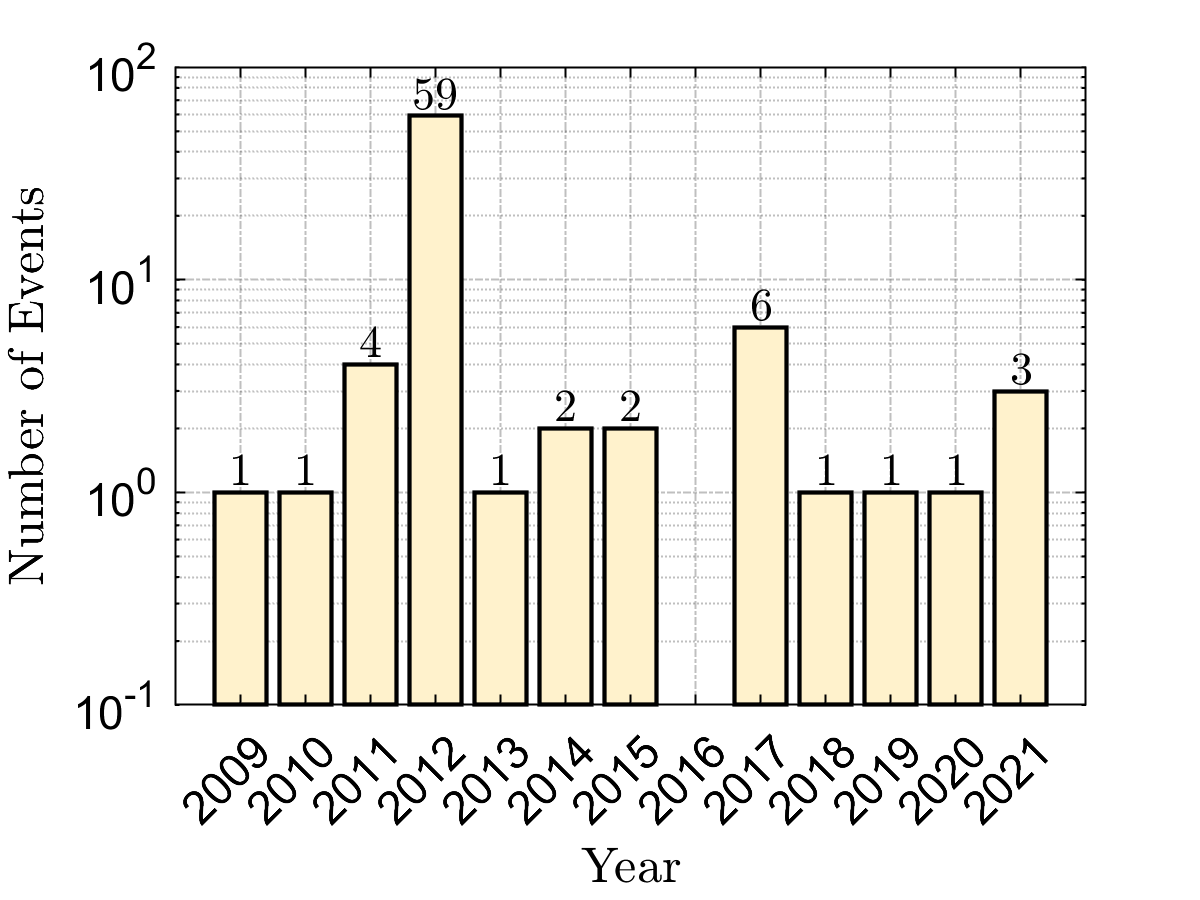
Figure 1: oscillation events per year

Figure 2: Oscillation events by country

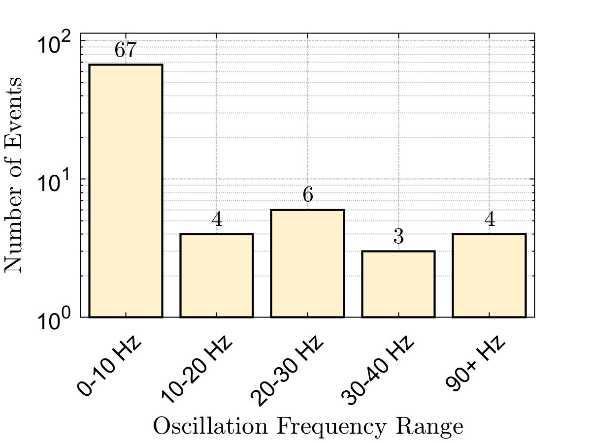
Figure 3: Oscillation events by frequency

Frequency scanning is a prevalent tool for analyzing power system stability, with researchers applying this method across various domains such as positive sequences, dq-frame, and alpha-beta domains. Additionally, different types of perturbation mechanisms, including multi-tone and single-tone, have been studied. Researchers have also explored various perturbation shapes such as step, ramp, and chirp. However, the explanation of frequency scanning results varies significantly throughout the research. Consequently, it is essential to categorize these methods systematically and compare them to identify the most suitable approach for specific applications. Therefore, this paper addresses these issues by providing the following contributions:

1. Provides a structured historical overview of SSR/SSO incidents linked to high IBR penetration, offering insights into emerging trends.

2. Unifies and categorizes existing stability analysis methods (white-, black-, and gray-box) for more informed method selection.

3. Systematically compares frequency scanning techniques and perturbation strategies, clarifying their advantages, limitations, and applications.

4. Delivers practical guidance for interpreting frequency scan results to identify instability risks and inform mitigation strategies.

Finally, the paper is organized as follows: Section II reviews the history of subsynchronous oscillations, Section III classifies IBR stability analysis methods, Section IV provides a detailed examination of frequency scanning techniques, Section V presents a broader discussion of frequency scanning insights, and Section VI concludes with the final remarks of this survey.

TABLE I: History of SSO events

No.	Year(s)	Location or Entity	Event Description	SSO Freq(Hz)	Ref
1	2007	South Central Minnesota	Type-3 WPP left radially connected to 345kV series compensated line	9.44	[21], [22]
2	2009	South Texas	Transmission line tripping left several type-3 WPPs connected to a 345-kV series-compensated line.	20-30	[21], [23]
3	2010	Oklahoma OG&E	Two wind farms output above 80% triggered oscillation	13	[24]
4	2011	Texas	Transmission line trip induced oscillation at type-4 WPP	4	[25]
5	2011-2014	Oregon (BPA)	Oscillations observed during high wind generation. 5-Hz and 14-Hz oscillations were detected in different periods.	5, 14	[24]
6	2011-2012	Oklahoma OG&E	Two 3Hz wind oscillation events were triggered due to line outages in 2011 and 2012.	3	[24]
7	2012-2013	North China	58+ oscillation events from type-3 WPPs’ interaction with 500-kV double circuit lines.	6-9	[26], [27]
8	2014-2015	Xinjiang China	30-Hz oscillations due to type-4 WPP interaction with 750kV weak grid system	30	[28]
9	2015	Hydro One, Canada	After the energizing of a 30-Mvar shunt capacitor at the substation.	20(Vrms), 80 (Iac)	[29]
10	2016	AEP footprint	PMUs captured oscillations for multiple days at a solar farm.	Not specified	[24]
11	2017	Northwest China	37-Hz and 63-Hz oscillations observed at a 600-MW type-3 WPP connected to a 220-kV weak grid	37, 63	[30], [31]
12	2017	First Solar’s solar farm, California	7-Hz oscillations in real power, reactive power, and RMS voltage.	7	[32]
13	2017	South Texas	Three separate SSO events occurred due to control software bug	22-26	[21]
14	2015-2019	Australia’s West Murray zone	7-Hz voltage oscillations due to low system strength and high IBR penetrations.	7	[33], [34]
15	2018-2019	Hydro One	3.5-Hz oscillations observed in real power and reactive power for planned 230kV outage which reduced system strength of type-4 WPP	3.5	[35]
16	2019	Great Britain (GB)	Weak grid trigger 9Hz oscillation 10 minutes before 2019 GB power system disruption and deload 800MW WPP	9	[36]
17	2020	West Murray zone, Australia	17-19 Hz voltage oscillations reported.	17-19	[37]
18	2021	Dominion Energy, eastern U.S.	22-Hz RMS voltage oscillations linked to a solar PV farm. 8-Hz and 82-Hz components were noted in currents and voltages.	22, 38, 82	[38]
19	2021	Scotland	8-Hz oscillations in RMS voltage observed on August 24, 2021. The system has high wind penetration.	8	[39]
20	2021	Kaua‘i’s power system	IBR induced system-wide 18-20Hz Oscillation	18-20	[40]
Acronyms: OG&E - Oklahoma Gas & Electric; BPA - Bonneville Power Administration; WF - Wind Farm; WPP - Wind Power Plant.

II Analysis of Recent SSO Events

As the penetration of renewable energy sources continues to grow, ongoing efforts to study and mitigate SSO will be crucial to ensure the stability and reliability of power systems worldwide. After reviewing literature [21], and IEEE PES TR-80 wind SSO task force report, all of these incidents are summarized in the Table I with the proper reference. Over the past two decades, the power industry has observed a significant increase in SSO events, particularly associated with wind and solar power generation. These events, spanning from 2007 to 2021, have been documented across various global regions, including the United States, Canada, China, Australia, Great Britain, and Scotland, underscoring the universal challenge SSO presents to power systems integrating renewable energy sources. Table I provides a detailed overview of these incidents, highlighting the location, event description, and oscillation frequency. The review of oscillation events from 2007 to 2021 highlights significant temporal, geographical, and frequency-specific trends depicted in Figs. 3–3.

Fig. 3 reveals that oscillation events are not evenly distributed over the years, with notable spikes such as the 59 events recorded in 2013. These peaks may correspond to systemic issues or technological transitions, such as large-scale wind and solar energy integration, which introduced new challenges in grid stability. Conversely, years with fewer events may reflect improvements in grid control systems or a lower intensity of renewable energy deployment.

Geographically, the distribution of events depicted in Fig. 3 emphasizes the influence of grid size, renewable energy adoption, and monitoring practices. China reports the highest number of SSO incidents (61), followed by the USA (16), while other countries, such as Australia, Canada, and the UK, report significantly fewer events. This disparity can be attributed to the extensive adoption of renewable energy technologies, such as wind farms, in China and the USA, as well as the corresponding grid complexities. Furthermore, the dominance of China in reported events highlights the challenges posed by high renewable energy penetration in large-scale interconnected power systems.

In terms of frequency presented in Fig. 3, the majority of oscillation events (67) occur within the 0–10 Hz range and often involve the inertial frequencies of synchronous generators. These low-frequency oscillations are commonly associated with interactions between renewable energy resources, weak grid conditions, and series-compensated transmission lines. Higher-frequency oscillations are becoming more prevalent, largely due to interactions between IBR controllers and the power grid. The characteristics of the bulk power grid can strongly influence these subsynchronous interactions, particularly in weak-grid situations or in cases where series or shunt capacitances create a grid resonance within this frequency range. We also anticipate that as renewable integration deepens, the overall spectrum of oscillation frequencies may shift upward, warranting further investigation.

Many occurrences were closely tied to weak grid conditions, high penetrations of Inverter-Based Resources (IBRs), and the presence of series-compensated lines. The oscillation frequencies recorded during these events varied widely, ranging from 3 Hz oscillation to several incidents exhibiting multiple frequency components. Several regions experienced repeated SSO events. For example, Oklahoma OG&E, South Texas, and the West Murray zone in Australia faced persistent issues. Notably, the West Murray zone dealt with prolonged challenges over four years (2015-2019), during which 7-Hz voltage oscillations were a persistent issue. In 2019, the Great Britain power system experienced a significant disruption, preceded by a 9 Hz oscillation, highlighting the potential severity of these events. In another notable incident in 2021, a solar PV farm at Dominion Energy in the eastern U.S. was linked to 22 Hz RMS voltage oscillations, showcasing the relevance of SSO issues in solar energy[38].

The triggering conditions for these SSO events were diverse, ranging from transmission line trips, high wind generation, and control software bugs to general grid weaknesses. This diversity highlights the complexity of SSO phenomena and the necessity for a multifaceted approach in analysis and mitigation.

TABLE II: Classification of Different Approaches of Stabality Analysis

Type	Method	Pros	Cons	Ref
White-box	State-space	Detailed insights into system dynamics	Requires system knowledge	[41] [42] [43] [44] [45] [46] [47] [48] [49]
	Transfer function based	Suitable for linear systems	Not ideal for non-linear systems	[50] [51] [52] [53] [54]
	Impedance Model	Provides frequency-domain insights	Challenging for complex systems	[55] [56] [52] [46] [57] [28]
	EMT Simulation	Accurate time-domain simulation	Computationally intensive	[53] [28] [58]
Black-box	Frequency scanning	Does not require system knowledge	Limited to frequency domain	[10] [59] [60] [15] [61] [62] [63] [64] [16] [12] [65] [13] [66] [67] [68] [11] [69] [70] [71] [72]
	Vector Fitting Method	Robust for high-order systems	Can be complex to implement	[73]
	Eigen System Realization	Effective for modal analysis	Requires data preprocessing	[74]
	Dissipating Energy Flow	Insightful for energy distribution	Limited by measurement accuracy	[40] [75] [76]
Grey-box	Combines model knowledge and data-driven methods	Requires both system knowledge and data	-	[77] [78]

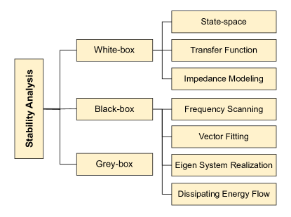
Figure 4: Classificaiton of IBR Stability Analysis

III Stabality Analysis

Identifying the possible oscillation is the key factor of stable grid operation. Investigating the origins of oscillations associated with IBR presents a multifaceted challenge. This complexity is attributed to the disparate IBR controller designs sourced from numerous vendors, coupled with the restricted access to, or the proprietary nature of, well-validated IBR models [40].

Existing literature explored different approaches to identify the oscillation. In this papers, all of those approaches are categorized under white-box, black-box, and gray-box. After carefully reviewing, a comprehensive categorization is presented in Fig. 4. The white-box approach considers that the whole system is known, containing physical and control parameters. White-box stability analysis is categorized down into eigenvalue analysis using state-space modeling [42, 43, 44, 45, 46, 47, 48, 49] , transfer function based analysis [50, 51, 52, 53, 54] , impedance model-based analysis [55] [56] [52] [46] [57] [28] and EMT simulation [53, 28, 58]. On the other hand, black-box IBR models are provided in binary format by the manufacturer, which can be solved in time-domain simulation and represent non-linear dynamics with high fidelity. Different literature analyzed the black-box model’s sub-synchronous oscillation in different ways. These methods includes frequency scanning [10, 59, 60, 15, 61, 62, 63, 64, 16, 12, 65, 13, 66, 67, 68, 11, 69, 70, 71, 72], Vector Fitting (VF) method [73], Eigen System Realization [74] and Dissipating Energy Flow [40, 75, 76].

The system operator prefers white-box IBR models for stability analysis. White-box models are state-space equations containing all of the physical control and system states. The state equation yields eigenvectors and the participation factor, which indicates the responsible state for oscillation. Therefore, to bridge the gap between black-box models by manufacturer and white-box model desired by the system operator, multiple literatures [77, 78] put an effort into building a gray-box approach that connects the gap between two methods.

Fig. 4 summarizes the primary stability assessment approaches and their supporting literature. Two frequently employed techniques for IBR stability analysis are eigenvalue-based state-space methods (white-box) and impedance-based frequency scanning methods (Bode or Nyquist plots). Each approach has inherent trade-offs: state-space modeling demands detailed, open-form converter models-which may not be available for proprietary systems-and requires re-linearization for every structural change, while frequency scanning is computationally intensive and sensitive to measurement noise. Given the nonlinear nature of power electronic converters, white-box modeling often involves complex linearization around specific operating points. Current literature shows these two methods dominate practical application, although hybrid (gray-box) approaches are emerging to bridge their respective limitations. The following section provides a detailed categorization of frequency scanning techniques.

IV Frequency Scanning and Stabality Analysis

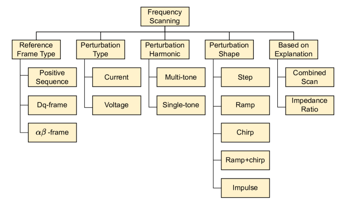
Figure 5: Frequency scanning classifications and different methods

Frequency scanning proved to be a prevalent tool for characterizing IBR and power systems. Existing literature [10, 59, 60, 15, 61, 62, 63, 64, 16, 12, 65, 13, 66, 67, 68, 11, 69, 70, 71, 72] explored mainly three types of frequency scanning techniques such as (1) positive sequence (ps), (2) dq-frame, and (3) $\alpha\beta$-frame scanning . Ref. [69] shortly explained three types of scannings and their relative advantage and computation complexities and feasibility in characterizing IBRs and generators. The dimensionality of the frequency-dependent model obtained varies based on the reference frame selected. The positive-sequence impedance model is a Single-Input Single-Output (SISO) system, while both $dq$ and $\alpha\beta$ impedance models are Multiple-Input Multiple-Output (MIMO) systems. Nonetheless, the scanning procedures for these three methods are identical. However, extracting a SISO impedance can be accomplished with a single scan. In contrast, a MIMO impedance necessitates separate perturbations for each axis, such as the d and q-axis separately [69]. Ref. [69] also suggested not all types of frequency scans are suitable for a specific application. Such as the ref. [69] suggested that the dq-scan provides the highest accuracy for full-size converter-based wind power systems (type-4). Fig. 5 depicts the classification of frequency based on recent literature. The classification is presented based on different categories. In the subsequent sections, the categorization will be explained briefly.

IV-A Frequency Scanning Mechanism

The fundamental steps of the frequency scanning procedure remain consistent regardless of the chosen reference frame (positive sequence, dq-frame, or $\alpha\beta$-frame), perturbation type (voltage or current), perturbation shape (step, ramp, chirp), or scanning approach (single-tone or multi-tone). Figs. 6, 8, and 8 illustrate examples of positive-sequence scanning, voltage-source perturbation, and current-source perturbation, respectively. Additional details on single-tone and multi-tone scanning techniques can be found in Subsections IV-D1 and IV-D2. The general procedure, as widely adopted in literature (e.g., [64]), is summarized as follows:

1. Establish Steady-State Conditions: Begin by running the system under its normal operating point until it reaches steady state. It is crucial that the system operates in a linear region around this point to ensure the validity of small-signal perturbation and linearization-based methods.

2. Inject Perturbation: Superimpose a small, sinusoidal perturbation of known frequency on the system’s voltage or current. The perturbation amplitude must be large enough to provide a good signal-to-noise ratio, yet small enough to avoid driving the system into non-linear regions. Record the resulting voltage and current waveforms at the point of interest.

3. Frequency Domain Analysis: Apply a Fast Fourier Transform (FFT) to the measured signals to extract voltage and current phasors at the injection frequency. The corresponding impedance at that frequency is then computed as $Z(f)=V(f)/I(f)$. The detailed steps for FFT-based amplitude extraction are presented in Algorithm 1.

4. Frequency Sweep: Repeat the perturbation and measurement process over a range of frequencies to build a full impedance profile. For example, to cover 0–120 Hz at a resolution of 0.5 Hz, systematically inject perturbations at each discrete frequency and record the resulting voltage abd current and post-process for impedance.

This iterative, frequency-by-frequency scanning procedure ultimately yields a frequency-dependent impedance model of the subsystem, enabling stability assessments and resonance analysis.

Algorithm 1 FFT Interpretation for Amplitude Extraction

1:Sampling frequency $F_{s}$, Number of samples $N$, FFT result $X(k)$

2:Frequency vector and Amplitude spectrum

3:Step 1: Get Amplitude from FFT Bin

• Calculate amplitude: $|X(f_{k})|=|X(k/N)|$

4:Step 2: Discard Negative Part of Spectrum

• Identify two-sided spectrum

• Discard the second half of the array

• Multiply remaining points by 2, except DC at 0Hz

5:Step 3: Convert Bin to Frequency

• Calculate total number of frequency points: $\frac{N}{2}$

• Calculate frequency interval: $\Delta f=\frac{F_{s}}{N}$

• Construct frequency vector: $[0:\Delta f:(\frac{F_{s}}{2}-\Delta f)]$

6:Output: Frequency vector and Single-sided Amplitude spectrum

IV-B Frequency Scanning: Reference Frame Type

In frequency scanning, three main types of reference frames are commonly used to analyze system behavior: positive sequence frequency scanning, dq-frame frequency scanning, and $\alpha\beta$-frame frequency scanning.

IV-B1 Positive Sequence Scanning

Positive sequence scanning (ps-scan) is a crucial technique in power systems analysis, especially for studying the impedance characteristics of IBR connected to weak grids or compensated networks [16]. The positive sequence impedance model is a Single-Input Single-Output (SISO) system, providing a simplified representation of the system’s behavior at the perturbation frequency.

Fig. 6 depicts the ps-scanning mechanism for HVDC wind farm system. This method leverages the application of sinusoidal perturbation signals in the sequence domain to derive the impedance of the converter subsystem based on the positive sequence components of the voltage and current signals at the point of interconnection (POI).

The relationship between the three-phase voltages ($V_{a},V_{b},V_{c}$) and the sequence components ($V_{0},V_{1},V_{2}$) is expressed through a transformation matrix. Specifically, the three-phase voltages can be represented as:

$$\begin{pmatrix}V_{a}\\ V_{b}\\ V_{c}\end{pmatrix}=\begin{pmatrix}1&1&1\\ 1&a^{2}&a\\ 1&a&a^{2}\end{pmatrix}\begin{pmatrix}V_{0}\\ V_{1}\\ V_{2}\end{pmatrix}$$ (1)

where $a=-\frac{1}{2}+\frac{\sqrt{3}}{2}i$ represents a complex operator corresponding to a 120-degree phase shift. Within this context, the positive sequence component ($V_{\text{1}}$) is calculated using the formula:

$$V_{1}=\frac{1}{3}(V_{a}+aV_{b}+a^{2}V_{c})$$ (2)

This equation accurately determines the positive sequence component from the three-phase phasors, providing a reliable means to analyze the system.

The ps-scan technique follows a structured process to extract impedance information. Initially, the scanned grid is brought to a steady-state condition. Following this, a positive-sequence voltage at the desired frequency, $V_{\text{inj}}(f)$, is injected between the equivalent source and the grid terminals. Subsequently, the voltage ($V_{\text{abc}}$) and current ($I_{\text{abc}}$) at the grid terminals are measured. The Fast Fourier Transform (FFT) is then applied to both $V_{\text{abc}}$ and $I_{\text{abc}}$ to obtain their phasor values at the frequency of the injected voltage, $V_{\text{inj}}(f)$. Then, the positive sequence component is calculated for both voltage and current using the equation 2. Finally, the positive sequence impedance ($Z_{1}(f)$) is calculated for each perturb frequency using the relation:

$$Z_{1}(f)=\frac{V_{1}(f)}{I_{1}(f)}$$ (3)

In this scenario, $V_{\text{abc}}$ is considered a phase-to-ground voltage, while $I_{\text{abc}}$ represents the current measured at the same phase.

A significant advantage of the positive sequence scanning technique is its computation speed, which is faster than that of dq and $\alpha\beta$ scanning methods [69][79]. This efficiency makes ps-scan a preferred choice for impedance extraction in power systems, ensuring quick and accurate analysis, crucial for the safe and reliable operation of wind power plants and associated transmission systems.

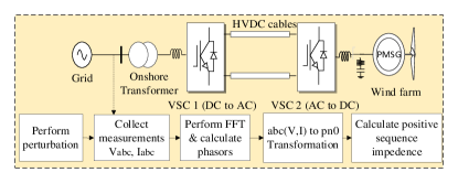
Figure 6: Procedure of performing positive sequence frequency scanning

TABLE III: Comparison between ps-scan, dq-scan, and $\alpha\beta$-scan methods

Item	ps-scan	dq-scan	$\alpha\beta$-scan
Stability criterion	Bode plot	Nyquist criterion	Generalized Nyquist criterion
Parameter	$Z_{ps}(f)$ and $Z_{ps}(c)(f)$	$L(f)$ in dq-frame	$L(f)$ in $\alpha\beta$-frame
Prediction reliability	Good, depends on impedance model accuracy	Very good, captures dq coupling, depends on impedance ratio accuracy	Good, depends on eigenvalue accuracy
Stability margin	Yes, visualized	Yes	Yes
Oscillation frequency	Magnitude intersection	Intersection with the unit circle	Intersection of dominant eigenlocus with the unit circle
Computational burden	Lowest	Generally, 2 × equivalent ps-scan	2 × equivalent ps-scan

IV-B2 dq-frame Frequency Scanning

The relationship between $dq$-currents and $dq$-voltages is represented by:

$$\begin{bmatrix}i_{d}(s)\\ i_{q}(s)\end{bmatrix}=\boldsymbol{Y}_{dq}(s)\begin{bmatrix}v_{d}(s)\\ v_{q}(s)\end{bmatrix}=\begin{bmatrix}Y_{dd}(s)&Y_{dq}(s)\\ Y_{qd}(s)&Y_{qq}(s)\end{bmatrix}\begin{bmatrix}v_{d}(s)\\ v_{q}(s)\end{bmatrix}$$ (4)

where $i_{d}(s)$ and $i_{q}(s)$ are the $dq$-currents, $v_{d}(s)$ and $v_{q}(s)$ are the $dq$-voltages, and $\boldsymbol{Y}_{dq}(s)$ is the $dq$-admittance matrix. This equation captures the coupling in the $dq$-frame, which sequence and $\alpha\beta$-scans might misrepresent in certain grid components[80][81][82]. The scanning procedure begins with the converter, where a step change is applied to the d-axis voltage, and the resulting dq-currents are measured at different frequencies. The process is repeated for the q-axis voltage. These signals are then transformed from the dq-frame back to the abc-frame using a dq-to-abc transformation and injected into the grid for further analysis. After measuring the currents and voltages in the abc-frame, the data is converted back to the dq-frame for Fourier analysis. The admittance components are computed as follows:

$$Y_{dd}(f_{i})=\frac{i_{d}^{d}(f_{i})}{v_{d}^{d}(f_{i})}, Y_{dq}(f_{i})=\frac{i_{d}^{q}(f_{i})}{v_{q}^{q}(f_{i})},$$ (5)

$$Y_{qd}(f_{i})=\frac{i_{q}^{d}(f_{i})}{v_{d}^{d}(f_{i})}, Y_{qq}(f_{i})=\frac{i_{q}^{q}(f_{i})}{v_{q}^{q}(f_{i})}.$$

For grid scanning, a similar current injection approach is employed, and the grid’s impedance is calculated using the same methodology. The resulting impedance values for the d- and q-axes can be expressed as:

$$Z_{dd}(f_{i})=\frac{v_{d}^{d}(f_{i})}{i_{d}^{d}(f_{i})}, Z_{dq}(f_{i})=\frac{v_{d}^{q}(f_{i})}{i_{q}^{q}(f_{i})},$$ (6)

$$Z_{qd}(f_{i})=\frac{v_{q}^{d}(f_{i})}{i_{d}^{d}(f_{i})}, Z_{qq}(f_{i})=\frac{v_{q}^{q}(f_{i})}{i_{q}^{q}(f_{i})}.$$

For system stability analysis, the loop gain is subsequently calculated via the Generalized Nyquist Criterion (GNC). Specifically, the loop gain-defined as the product of the grid’s dq-impedance and the converter’s dq-admittance—is given in Equation 15.

IV-B3 $\alpha\beta$-frame Frequency Scanning

The $\alpha\beta$-scan procedure is employed to deduce the small-signal transfer functions that map the input currents (or voltages) to the output voltages (or currents) within the steady $\alpha\beta$ reference frame [69][83]. Aside from the transformations applied, this method is analogous to the $dq$-scan previously explained.

The impedance on the grid side in the $\alpha\beta$-frame can be converted from the phasor-domain scan using the equation:

$$\mathbf{Z}_{g}^{\alpha\beta}(f)=\mathbf{T}_{C^{\prime}}\cdot\begin{bmatrix}Z_{g}^{ps}(f)&0\\ 0&Z_{g}^{ps*}(-f)\end{bmatrix}\cdot\mathbf{T}_{C^{\prime}}$$ (7)

where $\mathbf{T}_{C^{\prime}}=\frac{1}{\sqrt{2}}\begin{bmatrix}1&j\\ 1&-j\end{bmatrix}$, and $\mathbf{T}_{C^{\prime}}$ represents the complex transformation matrix.

Concurrently, the scan on the converter side gauges the $\alpha\beta$ admittance of the converter, represented as:

$$\mathbf{Y}_{c}^{\alpha\beta}(f)=\begin{bmatrix}Y_{\alpha,\alpha}(f)&Y_{\alpha,\beta}(f)\\ Y_{\beta,\alpha}(f)&Y_{\beta,\beta}(f)\end{bmatrix}$$ (8)

with $Y_{j,k}(f)=\frac{I_{j}(f)}{V_{k}(f)}$, where $j,k\in\{\alpha,\beta\}$. Here, $I$ and $V$ denote current and voltage, respectively, and the subscripts signify the respective measured and perturbed axes.

IV-C Perturbation Type: Voltage or Current

The scanning of grid-following Inverter-Based Resources (IBRs) can be conducted using perturbations in either voltage or current. Essentially, the two approaches produce results that are almost identical [69]. In practical applications, the technique of injecting current is more commonly utilized for frequency scanning on the grid side. In contrast, voltage perturbation is predominantly employed for frequency scanning on the Wind Turbine Generator (WTG) [64].

The scanning mechanism is the same for both cases. However, the connection of voltage and current source is different. It is essential to have the perturb voltage source connected to the series with the grid voltage shown in Fig. 8; therefore, the perturbation signal is superposed on the system voltage. On the other hand, current perturbation is injected into the grid in a parallel connection as depicted in Fig. 8. A fraction of the perturbation current flows into the grid. If the grid impedance is much smaller than the converter, this might affect the operating point of the system studied [69].

Typically, voltage injection is used for shunt-connected devices like STATCOMs, SVCs, and HVDCs, while current injection is preferred for series-connected devices such as TCSCs and SSSCs. Regardless of the injection method, the scanned subsystem must maintain a stable simulation to capture the frequency response accurately. Voltage perturbation scanning is more applicable in systems where voltage stability is a concern, such as weak grids or systems with high renewable energy penetration. In contrast, current perturbation scanning is often used in grids dominated by power electronics or systems with significant inverter-based resources. These two techniques complement each other, often being used together for a thorough assessment of system dynamics and stability.

IV-D Perturbation Harmonic

Two types of perturbation harmonics are found in the literature, i.e., single-tone and multi-tone. In a single-tone scan, a single-frequency sinusoidal is perturbed and records the output voltage and current. On the other hand, in the multi-tone method, multiple frequency signals are added together to form the perturbing signal.

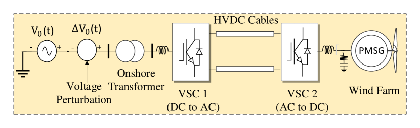
Figure 7: Voltage perturbation

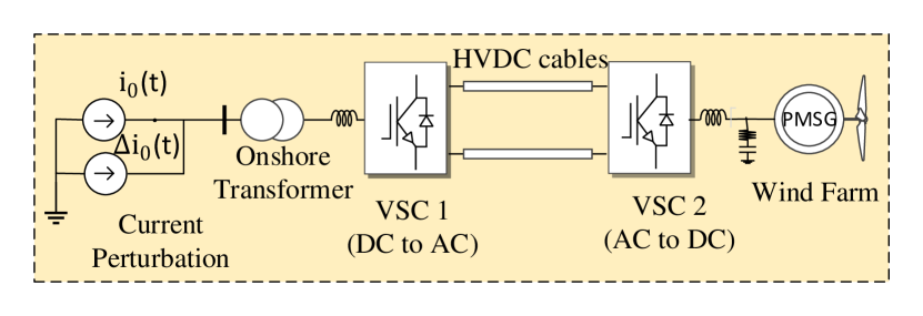
Figure 8: Current perturbation

IV-D1 Single-Tone Frequency Scanning

In single-tone frequency scanning, a single-frequency perturbation signal is injected during each measurement interval. For IBR characterization, a voltage-based perturbation is commonly employed, while current-based perturbation is used for grid characterization. The resulting impedance profile is then obtained by combining the voltage and current scan results.

A key drawback of this approach is the time required to cover a broad frequency range. For instance, scanning from 0 to 120 Hz at 0.5 Hz intervals would necessitate 240 individual perturbations (at 0 Hz, 0.5 Hz, 1.0 Hz, and so forth). While multi-tone injection can expedite the scanning process, Lwin et al. [84] provide evidence that simple single-tone sinusoidal perturbations are often more effective, especially when dealing with proprietary or manufacturer-specific black-box IBR models.

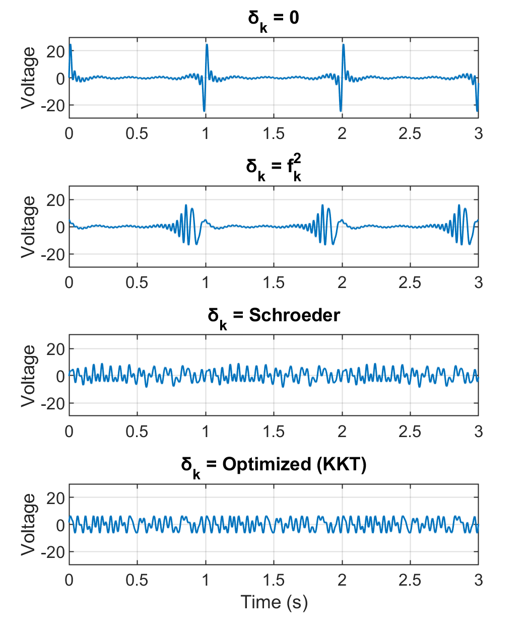
Figure 9: Multi-tone perturbation signal (Multi-sine Voltage Injection with Different Phase Shifts)

IV-D2 Multi-tone Frequency Scan

Multi-tone frequency scanning is an advanced method used to analyze the behavior of a system across multiple frequencies at the same time. Instead of testing one frequency at a time, as is done in single-tone scanning, this technique involves injecting a signal that contains several different frequencies simultaneously. This allows for a more comprehensive and efficient analysis of the system’s frequency response, making it easier to identify potential issues like resonances or instabilities across a wide range of frequencies. The process begins with generating a multi-tone signal, which is created by combining several sinusoidal waveforms, each representing a different frequency. These frequencies are carefully selected to cover the entire range of interest without interfering with each other. Once the multi-tone signal is ready, it is injected into the system at specific points, such as at a bus or a component that needs to be analyzed. The system’s response to this injection is then measured at various locations. The next step is to transform the measured response from the time domain to the frequency domain using a technique like the Fast Fourier Transform. This step breaks down the complex response into its frequency components, allowing engineers to see how the system behaves at each of the injected frequencies. By examining the amplitude and phase response at these frequencies, they can detect any problematic areas, such as points where the system might become unstable or resonant[85]. One of the main advantages of multi-tone scanning is its efficiency. Since multiple frequencies are analyzed at once, the scanning process is much faster than single-tone methods. Additionally, this approach provides a broader view of the system’s behavior, which is particularly useful in complex systems where problems might occur across a wide frequency range[85].

However, multi-tone scanning also comes with multiple challenges–primarily accurate signal identification and controlling the crest factor. The design of the multi-tone signal must be precise to avoid interference between tones, and interpreting the results is more complex due to the presence of multiple frequencies, which require careful analysis to separate and understand the system’s response [85]. To address the crest-factor issue, Matsuo [11] presented an optimization technique (Fig. 9) that applies an algorithm to find the optimum phase and minimize the crest factor; Table IV shows that Method 4 achieves the lowest peak and crest factor.

TABLE IV: Peak, RMS, and Crest Factor Values

Method	Peak	RMS	CF
Method 1	25.06	3.94	6.36
Method 2	16.31	3.94	4.14
Method 3	9.17	3.94	2.33
Method 4	6.42	3.94	1.63

Finally, Trevisan et al. [13] reference the work of Francis [86] to discuss the consequences associated with the use of multi-tone injections. However, they also acknowledge the research by Lwin et al. [84], which presents evidence suggesting that simpler, single-tone sinusoidal perturbations are more efficacious when dealing with models that are tailored to specific manufacturers.

IV-E Perturbation Shape

(a) Impulse perturbation

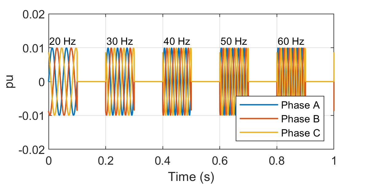
(b) Step perturbation

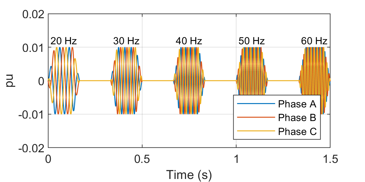
(c) Ramp perturbation

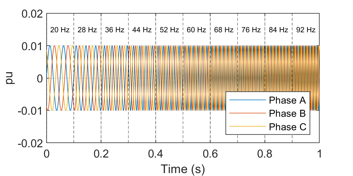
(d) Chirp perturbation

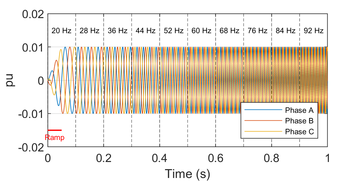
(e)Ramp+chirp perturbation

Figure 10: Different types of perturbation signals.

The perturbation properties, such as its frequency, waveform shape, and magnitude, serve as crucial parameters within the procedure [13]. By carefully selecting these parameters, researchers ensure that the induced responses accurately capture the underlying system dynamics, thereby improving the reliability of subsequent parameter estimation, system identification, and model validation processes [87, 88]. Based on the literature, five primary types of perturbation shapes have been identified: step, ramp, chirp, ramp+chirp, and impulse.

IV-E1 Impulse Perturbation

Impulse perturbations, as depicted in Fig. 10(a), momentarily inject a broadband excitation that encompasses multiple frequencies simultaneously and with equal phase. This sharp, instantaneous signal can quickly reveal certain resonance points and dynamic peculiarities, making it relatively straightforward to implement and interpret in simple systems. However, the large amplitude spikes produced by impulse perturbations may disturb normal system operations and compromise safety. Such abrupt stimuli often generate strong nonlinear effects, thus complicating the extraction of accurate frequency-response information. Given these limitations, the impulsive approach is rarely favored when more nuanced or stable testing methods are available [89, 4].

IV-E2 Step Perturbation

Step perturbations involve abrupt changes in frequency or amplitude at discrete intervals, creating stable plateau-like segments from which steady-state responses can be easily observed. As illustrated in Fig. 10(b), this approach simplifies the identification of how a system behaves under different fixed-frequency conditions, making it well-suited for preliminary assessments of system dynamics and stability. Despite these advantages, the sudden transitions associated with step perturbations can activate nonlinear system behaviors and introduce unwanted measurement noise [90]. This complication makes it more challenging to obtain smooth frequency response curves and to distinguish subtle resonance effects. While step perturbations remain a useful starting point, their inherent abruptness often limits their utility in scenarios demanding detailed frequency-response insights [13, 90].

IV-E3 Ramp Perturbation

Ramp perturbations gradually alter the frequency or amplitude of the input signal over time, as shown in Fig. 10(c). By providing a smoother transition between operating points, ramp signals reduce the likelihood of inciting nonlinearities and result in more stable conditions for testing. This characteristic makes ramp perturbations particularly attractive for systems where preserving stable operation and obtaining subtle resonance information is essential. However, the slower transitions inherent in ramp-based testing can increase the duration of experiments, and the continuous nature of the frequency variation necessitates careful analysis to extract the underlying frequency-response data. Despite these drawbacks, ramp perturbations strike a workable balance between simplicity and stability, rendering them a suitable option for more refined frequency-response analyses [13].

IV-E4 Chirp Perturbation

Chirp perturbations, depicted in Fig. 10(d), continuously vary their frequency content, enabling a comprehensive exploration of a system’s response across a broad frequency spectrum. This approach provides a richer, more continuous mapping of system dynamics than step or ramp perturbations, making it easier to identify resonant frequencies and other frequency-dependent phenomena without resorting to multiple isolated tests. However, the complexity of generating and interpreting chirp signals is higher, and the test duration tends to be longer. Extracting precise frequency-response information requires careful data processing and interpretation, given the continuously changing excitation frequency. While these factors increase the methodological difficulty, chirp perturbations are a powerful method that can yield detailed insights into system behavior that simpler perturbation methods are likely to miss [91, 92].

IV-E5 Ramp+Chirp Perturbation

The ramp+chirp perturbation, shown in Fig. 10(e), combines the smoothness of a ramp function with the broad frequency coverage of a chirp signal. By introducing the chirp within a controlled ramp, the method provides a gentler frequency trajectory than a pure chirp, thus reducing abruptness and lowering the risk of triggering nonlinear responses. While this hybrid approach offers improved stability and a more comprehensive examination of the system’s dynamic characteristics, it also elevates complexity in signal design, data processing, and interpretation. Increased testing times and more involved parameter extraction procedures are often necessary. Nevertheless, the ramp+chirp perturbation stands as a sophisticated option for studies requiring both smooth transitions and a wide frequency sweep, delivering high-quality insights into complex system behaviors [13].

IV-F Explaning Frequency Scanning Result

Frequency scanning identifies resonance spots in a system, where the impedance magnitude reaches peaks or troughs. These points are essential because they could indicate operational instability, harmonic amplification, or negative interactions between grid-connected components and their controls. When the reactance crosses from negative to positive, that frequency is called the crossover frequency for series resonance. Similarly, when the reactance crosses from positive to negative, that frequency is called the crossover frequency for parallel resonance [11, 64]. In addition, frequency scan data can illustrate how system strength affects impedance characteristics. For example, impedance profiles in strong grids are relatively flat, and the system behaves stable and well-damped over a wide frequency range meanwhile frequency scanning frequently reveals greater impedance magnitudes, more prominent resonance peaks, and shifts in resonance frequencies for weak grids, suggesting heightened susceptibility to disturbances, emphasizing the possibility for voltage instability and control interactions [93]. In the case of harmonics, frequency scanning offers information about the propagation and amplification of harmonics within a system. Peaks in impedance profiles at specific harmonic frequencies indicate the presence of harmonic resonance, which can result in power quality concerns, equipment overheating, and operational inefficiencies.

Existing literature [10, 59, 60, 15, 61, 62, 63, 64, 16, 12, 65, 13, 66, 67, 68, 11, 69, 70, 71, 72] explained frequency results differently. The representation also varies depending on the reference frame the scanning was performed. The interpretation of the results could be categorized mostly by a combined scan- and impedance ratio-based explanation. Both methods have advantages and disadvantages. The combined scan method includes the analysis of Impedance Over Frequency (Z-F), Admittance Over Frequency (Y-F), Phase Angle, and Nyquist Plots. On the other hand, the impedance ratio-based method involves the use of the Generalized Nyquist Criteria and Bode plots for analysis.

IV-F1 Combined Scans Analysis

Figure 11: Combined frequency scan procedure

The combined scan method is adopted in many parts of the literature to explain the stability of the overall system [13]. Figure 11 depicts the combined scan procedure. For the point of interconnection (POI), this method computes a frequency-dependent combined impedance of the grid and grid-connected inverters (GCIs). Small voltage or current disturbances are injected into the POI at various frequencies, and the positive sequence frequency-dependent impedances of the grid and the inverter-based resources (IBRs) are extracted from the measured voltages and currents using the Fast Fourier Transform technique. Thus, the total frequency-dependent impedance is determined by adding the two impedances. There are mainly two distinct types of resonance mode: series and parallel resonance. While series resonance transmits the energy within the same branch, parallel resonance energy exchanges between different branches.

In a series RLC circuit and using $s=j\omega$ the equivalent impedance is:

$$Z_{\text{eq}_{\text{s}}}=R+sL+\frac{1}{sC}$$ (9)

The crossover frequency is where the imaginary part of $Z_{\text{eq}_{\text{s}}}$ becomes zero and its derivative w.r.t. $\omega$ is positive [11]. As $\omega$ increases, reactance transitions from capacitive to inductive, with resonance when $\omega L=1/\omega C$. For an input voltage $V_{\text{in}}$, the transfer function is:

$$H_{S}(s)=\frac{I(s)}{V_{\text{in}}(s)}=\frac{1}{Z_{\text{eq}_{\text{s}}}}=\frac{Cs}{LCs^{2}+RCs+1}$$ (10)

The system is unstable if the poles of the transfer function (eqn: 10) are located in the right-half plane. Since the denominator of (eqn: 10) is a quadratic equation, the real part of the poles is $\frac{-R}{2L}$. As a result, the stability of a series circuit would correlate with the resistance value at the resonance frequency.

On the other hand, parallel resonance would be identified if the reactance goes from positive (inductive) to negative (capacitive) when the frequency $\omega$ grows and it occurs when the inductive and capacitive admittances cancel each other. For parallel resonance, the equivalent impedance $Z_{\text{eq}_{\text{p}}}$ comprising a resistor ($R$), inductor ($L$), and capacitor ($C$) is calculated using the reciprocal of the total admittance:

$$\frac{1}{Z_{\text{eq}_{\text{p}}}}=\frac{1}{R}+\frac{1}{j\omega L}+j\omega C$$ (11)

Considering the input current source $I_{\text{in}}$, the transfer function of the parallel circuit would be:

$$H_{P}(s)=\frac{V(s)}{I_{\text{in}}(s)}=Z_{\text{eq}_{\text{p}}}=\frac{RLs}{RLCs^{2}+Ls+R}$$ (12)

The real component of the poles of the parallel transfer function (Equation 12) could be calculated as $\frac{-L}{2RLC}$. If the resistance of the parallel circuit is less than zero at the crossover frequency, the poles would be on the right-half plane, causing the parallel resonance mode unstable. Consequently, combined scan analysis can signify system stability depending on the polarity of the resistance value at the resonance frequency.

(a)

(b)

Figure 12: Combined scan result explanation mechanism (a) a simple circuit to demonstrate resonance (b) series and parallel resonance

To understand combined scan result, ref. [64] explained using a simple circuit demonstrated in Fig. 12 (a). These circuit parameters are hypothetically chosen to study the combined scan analysis. The example circuit operating with 60 Hz fundamental frequency comprises two subsystems. Fig. 12 (b) presents the reactance and resistance of the circuit with respect to frequency. Then the total impedance is the summation of the two and can be evaluated to gain insight to stability. Evaluating the impedance of an electrical system can help identify unstable resonance modes. For example, the circuit in Fig. 12 has two resonance modes at 12.99 Hz and 21.51 Hz where the reactance X crosses zero. The one at 12.99 Hz is a shunt resonance mode as X crosses zero from positive to negative, while the one at 21.51 Hz is a series resonance mode as X crosses zero from negative to positive. Evaluating the series resonance mode shows that it is unstable as the corresponding resistance R is negative. This can be understood by approximating the circuit as an equivalent RLC series branch. Considering the characteristic equation of such branch, negative resistance means that the pole is in the right half plane, therefore the circuit is unstable.

IV-F2 Impedance Ratio Based Stability Analysis

In power system analyses, it is often practical to partition the network into two subsystems: the element under investigation and the rest of the grid. By representing each subsystem as an equivalent impedance or admittance, an impedance ratio between them can be established [14, 94]. This impedance ratio has been demonstrated to correspond to the open-loop gain of the system [12, 95]. Each subsystem can be equivalent to the Thevenin or Norton circuit, as shown in the single-line circuit examples of Fig. 13 (a)–(b). The voltage at the PCC can be calculated as for the Norton circuit:

$$V =I_{1}\frac{1}{Y_{1}+Y_{2}}+I_{2}\frac{1}{Y_{1}+Y_{2}}=I_{1}\frac{Z_{1}}{1+Z_{1}Y_{2}}+I_{2}\frac{Z_{1}}{1+Z_{1}Y_{2}}$$ (13)

$$=I_{1}\frac{Z_{2}}{1+Z_{2}Y_{1}}+I_{2}\frac{Z_{2}}{1+Z_{2}Y_{1}}$$

(a) Norton circuit representation

(b) Thevenin circuit representation

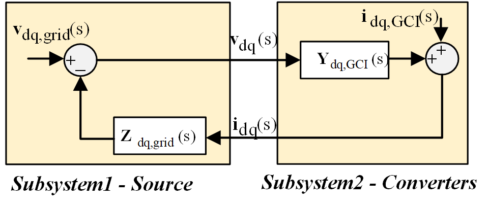
(c) dq-ISBA circuit representation

Figure 13: Cascaded system equivalent circuit

Similarly, the voltage at the PCC for the Thevenin circuit can be calculated:

$$V =\frac{Z_{2}V_{1}+Z_{1}V_{2}}{Z_{1}+Z_{2}}=\frac{V_{1}+\frac{Z_{1}}{Z_{2}}V_{2}}{1+\frac{Z_{1}}{Z_{2}}}=\frac{\frac{Z_{2}}{Z_{1}}V_{1}+V_{2}}{1+\frac{Z_{2}}{Z_{1}}}$$ (14)

In both Thevenin and Norton representations, the impedances of the subsystems are equivalent, such that $Z_{2}=Y_{2}^{-1}$ and $Z_{1}=Y_{1}^{-1}$, where $Y_{1}$ and $Y_{2}$ are the admittances of the respective subsystem. The impedance ratio $Z_{1}Y_{2}$ serves as the system’s open-loop transfer function and is utilized for stability analysis [96].

System stability can be evaluated by applying the Nyquist Stability Criterion (NSC) to $Z_{1}Y_{2}(s)$. The assumption that $Z_{1}Y_{2}(s)$ has no right-half plane (RHP) poles allows for stability analysis using only the Nyquist plot. Under these conditions, the system is stable if and only if the Nyquist plot of the impedance ratio does not encircle the critical point $(-1,j0)$.

The Impedance-Based Stability Criterion (IBSC) plays a pivotal role in analyzing the interactions between power converters and passive components [97, 98]. The IBSC uses terminal impedance/admittance characteristics of the grid’s impedance $Z_{\text{grid}}$ and the converters admittance $Y_{\text{CGI}}$ to find out the interconnected system stability. Referring to Fig. 13(a)–(b), Subsystem 1 is considered as the Source, and Subsystem 2 as Converters. A graphical representation of this analysis is depicted in Fig. 13(c).The stability of the interconnected system can be evaluated using the minor loop gain, defined matrix terms as:

$$\boldsymbol{L}(s)=\boldsymbol{Z}_{dq,\text{grid}}(s)\boldsymbol{Y}_{dq,\text{GCI}}(s)=\frac{\boldsymbol{Y}_{dq,\text{GCI}}(s)}{\boldsymbol{Y}_{dq,\text{Grid}}(s)}$$ (15)

Within stability analyses, both the magnitude criterion $|Y_{\text{CGI}}|>|Y_{\text{Grid}}|$ and the negative phase angle crossover criterion ($\angle Y_{\text{CGI}}-\angle Y_{\text{Grid}}=-\pi\pm 2\pi N$) must be satisfied [12, 95]. To apply this method effectively, certain prerequisites are required. The converter should maintain stability when it is unloaded or short-circuited to ground in the case of a current-controlled converter—and the grid must remain stable when the converter is disconnected [73]. Additionally, a significant challenge arises if the network contains nonlinear elements. In such scenarios, the impedance scan must be performed at the same operating point as when the converter is connected to the network, which can be difficult to achieve after disconnecting the converter [99].

Control theory emphasizes the importance of open-loop gain in stability analysis, especially when determining phase and gain margins. A system may become unstable if the impedance ratio introduces a phase shift of -180 degree at a frequency where the gain magnitude is equal to or exceeds unity. To extend the Nyquist stability criterion to Multiple Input Multiple Output (MIMO) systems, Gershgorin bands are utilized. These bands help identify critical gains that govern the gain and phase margins of closed-loop systems [100, 101]. The dq-scanning technique, integral to MIMO systems, aids in stability prediction through the Impedance-Based Stability Assessment (IBSA) theory. This method generates a 2x2 admittance matrix for the converter and a 2x2 impedance matrix for the grid at each evaluated frequency [102]. A transfer function matrix in the dq-domain, as described in Equation 15, is represented using the following notation:

$$\boldsymbol{L}(s)=\begin{bmatrix}L_{dd}(s)&-L_{qd}(s)\\ L_{dq}(s)&L_{qq}(s)\end{bmatrix}$$ (16)

where the negative sign in the (1,2) element is chosen to be consistent with the definition of complex vectors. When implementing the generalized Nyquist theorem to expand from SISO to MIMO systems, it takes into account multiple complex contours. These contours show the eigenvalue $\lambda_{i}(s)$ of $\boldsymbol{L}(s)$, evaluated at $s=j\omega$. The Nyquist paths are then formed by the eigen-loci of:

$$0=\det(\lambda I_{N}-\boldsymbol{L}(s))$$ (17)

Equation 17 defines the open-loop transfer function matrix $\boldsymbol{L}(s)$ in an electrical system, which includes both impedance and admittance matrices. To assess how impedance and admittance individually influence closed-loop stability, it is essential to separate the two eigenvalues $\lambda_{1},_{2}(s)$ as functions of their respective impedance and admittance components. By substituting 15 into 17, where $\boldsymbol{L}(s)$ is a $2\times 2$ transfer function matrix, separating the eigenvalues requires that one of the transfer function matrices (either $\boldsymbol{Y}_{dq,\text{GCI}}(s)$ or $\boldsymbol{Z}_{dq,\text{grid}}(s)$) must have zero entries for both $L_{dd}(s)$ and $L_{qq}(s)$ or both $L_{dq}(s)$ and $L_{qd}(s)$ (diagonal or antidiagonal). The Nyquist plot of the return ratio then gives useful information on the system’s stability, as shown in Figure 14.

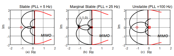
Figure 14: Example: Stability Assessment using MIMO Models [103]

Despite its utility, GNC has limitations, primarily providing only qualitative stability results (stable or unstable) without detailed explanations of instability causes. Furthermore, getting all of the required impedance responses is difficult due to the computing effort involved and the need to individually scan the network impedance with IBRs. To overcome these limitations, alternative stability criteria have been proposed. To support power networks with high levels of IBRs, the National Renewable Energy Laboratory (NREL) developed a Reversed Impedance-Based Stability Criterion (RIBSC) and the Grid Impedance Scan Tool (GIST) [104]. The Vector Fitting (VF) approach was also used to improve the IBSC [73]. Moreover, stability criteria based on the impedance-frequency characteristics of the impedance matrix determinant [105], and the nodal admittance matrix (NAM)-based criterion—which preserves the system’s inherent structure by leveraging the system admittance matrix—have been presented [106, 107]. These approaches offer more comprehensive insights into system stability.

V Discussion

This literature has explored various methodologies for analyzing SSO and system stability in power networks, with a focus on frequency scanning techniques and perturbation-based methods. Frequency scanning methods, categorized into positive-sequence, dq-frame, and $\alpha\beta$-frame scans, emerged as critical tools for understanding the dynamic interactions between grid components and IBRs. While the positive-sequence scan provides quick insights-offering an overall, high-level view of the system’s resonance points and potential areas of instability without delving into detailed dynamics-it is less accurate for converter-based systems, as it simplifies the system into a single sequence. The dq-frame scan is more precise for such systems, as it captures the coupling between axes. Multi-tone frequency scanning, though efficient for wide-range frequency analysis, presents challenges in designing perturbation signals and interpreting results due to interference between frequencies. The discussion around perturbation shapes, including ramp, chirp, and impulse perturbations, further emphasizes the importance of selecting appropriate perturbations to prevent non-linear responses and ensure accurate system analysis. The analysis of frequency scanning results through combined scan methods and impedance ratio-based approaches offers a robust understanding of the conditions leading to system instability. The review showed that while resonance frequencies indicate critical points in the system, it is the behavior of resistance at these frequencies that ultimately determines whether the system is stable. The combined scan method, which adds grid and IBR impedances, allows for a comprehensive view of system dynamics, whereas the impedance ratio method provides a more control-theory-driven approach using Nyquist Stability Criteria.

VI Conclusion

In conclusion, as power systems rapidly transition toward inverter-based resources, ensuring reliable and stable operation demands increasingly sophisticated analytical tools and methodologies. This survey has traced the evolution of stability challenges particularly subsynchronous resonance (SSR) and oscillation phenomena by reviewing past events and categorizing widely used modeling approaches into white-box, black-box, and gray-box frameworks. Among these, frequency scanning methods stand out as versatile and powerful tools, offering insights through positive-sequence, dq-frame, and $\alpha\beta$-frame analyses, along with various perturbation strategies such as single-tone, multi-tone, step, ramp, chirp, and combined ramp-chirp. When combined with impedance ratio-based interpretations and stability criteria (including Nyquist and Generalized Nyquist methods), frequency scanning enables a detailed understanding of system behavior and potential instability points. Ultimately, selecting appropriate scanning methods, perturbation shapes, and interpretation techniques is critical for operators and researchers seeking to identify, mitigate, and prevent adverse interactions in systems with high levels of renewable penetration.

References

- [1] IEA, “Tracking Clean Energy Progress,” https://www.iea.org/reports/renewables, 2022.
- [2] M. I. Blanco, “The economics of wind energy,” Renewable and Sustainable Energy Reviews, vol. 13, no. 6, pp. 1372–1382, Aug. 2009.
- [3] A. Mostafaeipour and N. Mostafaeipour, “Renewable energy issues and electricity production in Middle East compared with Iran,” Renewable and Sustainable Energy Reviews, vol. 13, no. 6, pp. 1641–1645, Aug. 2009.
- [4] A. Evans, V. Strezov, and T. J. Evans, “Assessment of sustainability indicators for renewable energy technologies,” Renewable and Sustainable Energy Reviews, vol. 13, no. 5, pp. 1082–1088, Jun. 2009.
- [5] L. Gross, “Sub-Synchronous Grid Conditions: New Event, New Problem, and New Solutions,” 2010.
- [6] IEEE, “Reader’s guide to subsynchronous resonance,” IEEE Transactions on Power Systems, vol. 7, no. 1, pp. 150–157, Feb. 1992.
- [7] J. W. Butler and C. Concordia, “Analysis of Series Capacitor Application Problems,” Transactions of the American Institute of Electrical Engineers, vol. 56, no. 8, pp. 975–988, Aug. 1937.
- [8] J. W. Ballance and S. Goldberg, “Subsynchronous Resonance in Series Compensated Transmission Lines,” IEEE Transactions on Power Apparatus and Systems, vol. PAS-92, no. 5, pp. 1649–1658, Sep. 1973.
- [9] L. Wang, X. Xie, H. Liu, Y. Zhan, J. He, and C. Wang, “Review of emerging SSR/SSO issues and their classifications,” The Journal of Engineering, vol. 2017, no. 13, pp. 1666–1670, 2017.
- [10] M. Elfayoumy and C. Moran, “A comprehensive approach for sub-synchronous resonance screening analysis using frequency scanning technique,” in 2003 IEEE Bologna Power Tech Conference Proceedings,, vol. 2. Bologna, Italy: IEEE, 2003, pp. 626–630.
- [11] I. B. M. Matsuo, F. Salehi, L. Zhao, Y. Zhou, and W.-J. Lee, “Optimized Frequency Scanning of Nonlinear Devices Applied to Subsynchronous Resonance Screening,” IEEE Transactions on Industry Applications, vol. 56, no. 3, pp. 2281–2291, May 2020.
- [12] Y. Liao and X. Wang, General Rules of Using Bode Plots for Impedance-Based Stability Analysis, Jun. 2018.
- [13] A. S. Trevisan, Â. Mendonça, R. Gagnon, J. Mahseredjian, and M. Fecteau, “Analytically Validated SSCI Assessment Technique for Wind Parks in Series Compensated Grids,” IEEE Transactions on Power Systems, vol. 36, no. 1, pp. 39–48, Jan. 2021.
- [14] J. Sun, “Impedance-Based Stability Criterion for Grid-Connected Inverters,” IEEE Transactions on Power Electronics, vol. 26, no. 11, pp. 3075–3078, Nov. 2011.
- [15] B. Badrzadeh, M. Sahni, Y. Zhou, D. Muthumuni, and A. Gole, “General Methodology for Analysis of Sub-Synchronous Interaction in Wind Power Plants,” IEEE Transactions on Power Systems, vol. 28, no. 2, pp. 1858–1869, May 2013.
- [16] U. Karaagac, J. Mahseredjian, S. Jensen, R. Gagnon, M. Fecteau, and I. Kocar, “Safe Operation of DFIG-Based Wind Parks in Series-Compensated Systems,” IEEE Transactions on Power Delivery, vol. 33, no. 2, pp. 709–718, Apr. 2018.
- [17] C. Buchhagen, C. Rauscher, A. Menze, and J. Jung, “BorWin1 - First Experiences with harmonic interactions in converter dominated grids,” in International ETG Congress 2015; Die Energiewende - Blueprints for the New Energy Age, Nov. 2015, pp. 1–7.
- [18] Y. Cheng, S. H. F. Huang, J. Rose, V. A. Pappu, and J. Conto, “Subsynchronous resonance assessment for a large system with multiple series compensated transmission circuits,” IET Renewable Power Generation, vol. 13, no. 1, pp. 27–32, 2019.
- [19] H. Saad, Y. Fillion, S. Deschanvres, Y. Vernay, and S. Dennetiere, “On Resonances and Harmonics in HVDC-MMC Station Connected to AC Grid,” IEEE Transactions on Power Delivery, vol. 32, no. 3, pp. 1565–1573, Jun. 2017.
- [20] N. Karnik, D. Novosad, H. K. Nia, M. Sahni, M. Ghavami, and H. Yin, “An evaluation of critical impact factors for SSCI analysis for wind power plants: A utility perspective,” in 2017 IEEE Power & Energy Society General Meeting, Jul. 2017, pp. 1–5.
- [21] I. PES, “Wind Energy Systems Sub-Synchronous Oscillations: Events and Modeling (TR80),” https://resourcecenter.ieee-pes.org/publications/technical-reports/PES_TP_TR80_AMPS_WSSO_070920.html, 2020.
- [22] A. Mulawarman, “Detection of Undamped Sub-Synchronous Oscillations of Wind Generators with Series Compensated Lines,” 2011.
- [23] G. D. Irwin, A. K. Jindal, and A. L. Isaacs, “Sub-synchronous control interactions between type 3 wind turbines and series compensated AC transmission systems,” in 2011 IEEE Power and Energy Society General Meeting, Jul. 2011, pp. 1–6.
- [24] North American Electric Reliability Corporation (NERC), “Reliability guideline: Forced oscillation monitoring and mitigation,” Sep. 2017, accessed: 2023-10-23.
- [25] S.-H. Huang, J. Schmall, J. Conto, J. Adams, Y. Zhang, and C. Carter, “Voltage control challenges on weak grids with high penetration of wind generation: ERCOT experience,” in 2012 IEEE Power and Energy Society General Meeting, Jul. 2012, pp. 1–7.
- [26] “IEEE PES WindSSO Taskforce, “PES TR-80: Wind Energy Systems Subsynchronous Oscillations: Events and Modeling,” Jul. 2020.
- [27] X. Xie, X. Zhang, H. Liu, H. Liu, Y. Li, and C. Zhang, “Characteristic Analysis of Subsynchronous Resonance in Practical Wind Farms Connected to Series-Compensated Transmissions,” IEEE Transactions on Energy Conversion, vol. 32, no. 3, pp. 1117–1126, Sep. 2017.
- [28] H. Liu, X. Xie, J. He, T. Xu, Z. Yu, C. Wang, and C. Zhang, “Subsynchronous Interaction between Direct-Drive PMSG Based Wind Farms and Weak AC Networks,” IEEE Transactions on Power Systems, vol. 32, no. 6, pp. 4708–4720, 2017.
- [29] C. Li, “Unstable Operation of Photovoltaic Inverter From Field Experiences,” IEEE Transactions on Power Delivery, vol. 33, no. 2, pp. 1013–1015, Apr. 2018.
- [30] I. Vieto, G. Li, and J. Sun, “Behavior, Modeling and Damping of a New Type of Resonance Involving Type-III Wind Turbines,” in 2018 IEEE 19th Workshop on Control and Modeling for Power Electronics (COMPEL), Jun. 2018, pp. 1–8.
- [31] J. Sun and I. Vieto, “Development and Application of Type-III Turbine Impedance Models Including DC Bus Dynamics,” IEEE Open Journal of Power Electronics, vol. 1, pp. 513–528, 2020.
- [32] M. Morjaria, “Deploying Utility-Scale PV Power Plants in Weak Grids.”
- [33] S. Shah, J. Lu, and N. Modi, “Identifying potential sub-synchronous oscillations using impedance scan approach: Preprint.” National Renewable Energy Laboratory (NREL), Golden, CO (United States), 08 2024. [Online]. Available: https://www.osti.gov/biblio/2439741
- [34] A. Jalali, B. Badrzadeh, J. Lu, N. Modi, and M. Gordon, “System strength challenges and solutions developed for a remote area of Australian power system with high penetration of inverter-based resources,” CIGRE Sci. Eng. J., pp. 27–37, 2021.
- [35] C. Li and R. Reinmuller, “Asset Condition Anomaly Detections by Using Power Quality Data Analytics,” in 2019 IEEE Power & Energy Society General Meeting (PESGM), Aug. 2019, pp. 1–5.
- [36] “GB power system disruption on 9 August 2019: Final report,” Final report.
- [37] “AEMO | System strength workshop,” https://aemo.com.au/en/learn/energy-explained/system-strength-workshop.
- [38] C. Wang, C. Mishra, K. D. Jones, R. M. Gardner, and L. Vanfretti, “Identifying Oscillations Injected by Inverter-Based Solar Energy Sources,” in 2022 IEEE Power & Energy Society General Meeting (PESGM). Denver, CO, USA: IEEE, Jul. 2022, pp. 1–5.
- [39] “G-PST/ESIG Webinar Series: Managing Grid Stability in a High IBR Network - ESIG,” https://www.esig.energy/event/webinar-managing-grid-stability-in-a-high-ibr-network/.
- [40] S. Dong, B. Wang, J. Tan, C. J. Kruse, B. W. Rockwell, and A. Hoke, “Analysis of November 21, 2021, Kaua‘i Island Power System 18-20 Hz Oscillations,” Feb. 2023.
- [41] A. Moharana, R. K. Varma, and R. Seethapathy, “SSR mitigation in wind farm connected to series compensated transmission line using STATCOM,” in 2012 IEEE Power Electronics and Machines in Wind Applications. Denver, CO, USA: IEEE, Jul. 2012, pp. 1–8.
- [42] A. Moharana, R. Varma, and R. Seethapathy, “SSR alleviation by STATCOM in induction-generator-based wind farm connected to series compensated line,” IEEE Transactions on Sustainable Energy, vol. 5, no. 3, pp. 947–957, 2014.
- [43] L. Fan, R. Kavasseri, Z. L. Miao, and C. Zhu, “Modeling of DFIG-Based Wind Farms for SSR Analysis,” IEEE Transactions on Power Delivery, vol. 25, no. 4, pp. 2073–2082, Oct. 2010.
- [44] Y. Xu, M. Zhang, L. Fan, and Z. Miao, “Small-Signal Stability Analysis of Type-4 Wind in Series-Compensated Networks,” IEEE Transactions on Energy Conversion, vol. 35, no. 1, pp. 529–538, Mar. 2020.
- [45] A. S. Trevisan, M. Fecteau, A. Mendonça, R. Gagnon, and J. Mahseredjian, “Analysis of low frequency interactions between DFIG wind turbines and series compensated systems.”
- [46] M. Amin and M. Molinas, “Small-Signal Stability Assessment of Power Electronics Based Power Systems: A Discussion of Impedance- and Eigenvalue-Based Methods,” IEEE Transactions on Industry Applications, vol. 53, no. 5, pp. 5014–5030, Sep. 2017.
- [47] D. H. R. Suriyaarachchi, U. D. Annakkage, C. Karawita, and D. A. Jacobson, “A Procedure to Study Sub-Synchronous Interactions in Wind Integrated Power Systems,” IEEE Transactions on Power Systems, vol. 28, no. 1, pp. 377–384, Feb. 2013.
- [48] K. Rauma, K. Md Hasan, C. Gavriluta, and C. Citro, “Resonance analysis of a wind power plant with modal approach,” in 2012 IEEE International Symposium on Industrial Electronics, May 2012, pp. 2042–2047.
- [49] Y. Li, L. Fan, and Z. Miao, “Wind in Weak Grids: Low-Frequency Oscillations, Subsynchronous Oscillations, and Torsional Interactions,” IEEE Transactions on Power Systems, vol. 35, no. 1, pp. 109–118, Jan. 2020.
- [50] C. Bajracharya and M. Molinas, “Understanding of tuning techniques of converter controllers for VSC-HVDC,” 2008.
- [51] K. M. Alawasa, Y. A.-R. I. Mohamed, and W. Xu, “Modeling, Analysis, and Suppression of the Impact of Full-Scale Wind-Power Converters on Subsynchronous Damping,” IEEE Systems Journal, vol. 7, no. 4, pp. 700–712, Dec. 2013.
- [52] K. M. Alawasa, Y. I. Mohamed, and W. Xu, “Active Mitigation of Subsynchronous Interactions Between PWM Voltage-Source Converters and Power Networks,” IEEE Transactions on Power Electronics, vol. 29, no. 1, pp. 121–134, Jan. 2014.
- [53] Hailian Xie and M. M. De Oliveira, “Mitigation of SSR in presence of wind power and series compensation by SVC,” in 2014 International Conference on Power System Technology. Chengdu: IEEE, Oct. 2014, pp. 2819–2826.
- [54] L. Sainz, L. Monjo, M. Cheah-Mane, and J. Liang, “Assessment of subsynchronous oscillations in AC grid-connected VSC systems with type-4 wind turbines,” IET Renewable Power Generation, vol. 13, no. 16, pp. 3088–3096, 2019.
- [55] L. Fan and Z. Miao, “Nyquist-Stability-Criterion-Based SSR Explanation for Type-3 Wind Generators,” IEEE Transactions on Energy Conversion, vol. 27, no. 3, pp. 807–809, Sep. 2012.
- [56] S. Chernet, M. Bongiorno, G. K. Andersen, T. Lund, and P. C. Kjaer, “Online variation of wind turbine controller parameter for mitigation of SSR in DFIG based wind farms,” in 2016 IEEE Energy Conversion Congress and Exposition (ECCE). Milwaukee, WI, USA: IEEE, Sep. 2016, pp. 1–8.
- [57] M. Amin and M. Molinas, “Understanding the Origin of Oscillatory Phenomena Observed Between Wind Farms and HVdc Systems,” IEEE Journal of Emerging and Selected Topics in Power Electronics, vol. 5, no. 1, pp. 378–392, Mar. 2017.
- [58] Y. Li, L. Fan, and Z. Miao, “Replicating Real-World Wind Farm SSR Events,” IEEE Transactions on Power Delivery, vol. 35, no. 1, pp. 339–348, Feb. 2020.
- [59] R. Nath and C. Grande-Moran, “Study of Sub-Synchronous Control Interaction due to the interconnection of wind farms to a series compensated transmission system,” in PES T&D 2012. Orlando, FL, USA: IEEE, May 2012, pp. 1–6.
- [60] M. Sahni, D. Muthumuni, B. Badrzadeh, A. Gole, and A. Kulkarni, “Advanced screening techniques for Sub-Synchronous Interaction in wind farms,” in PES T&D 2012, May 2012, pp. 1–9.
- [61] Y. Cheng, M. Sahni, D. Muthumuni, and B. Badrzadeh, “Reactance Scan Crossover-Based Approach for Investigating SSCI Concerns for DFIG-Based Wind Turbines,” IEEE Transactions on Power Delivery, vol. 28, no. 2, pp. 742–751, Apr. 2013.
- [62] S. Gupta, A. Moharana, and R. K. Varma, “Frequency scanning study of sub-synchronous resonance in power systems,” in 2013 26th IEEE Canadian Conference on Electrical and Computer Engineering (CCECE), May 2013, pp. 1–6.
- [63] B. Wen, “Stability Analysis of Three-phase AC Power Systems Based on Measured D-Q Frame Impedances,” Ph.D. dissertation, 2014.
- [64] W. Ren and E. Larsen, “A Refined Frequency Scan Approach to Sub-Synchronous Control Interaction (SSCI) Study of Wind Farms,” IEEE Transactions on Power Systems, vol. 31, no. 5, pp. 3904–3912, Sep. 2016.
- [65] A. Rygg and M. Molinas, “Apparent Impedance Analysis: A Small-Signal Method for Stability Analysis of Power Electronic-Based Systems,” IEEE Journal of Emerging and Selected Topics in Power Electronics, vol. 5, no. 4, pp. 1474–1486, Dec. 2017.
- [66] L. Fan, Z. Miao, P. Koralewicz, S. Shah, and V. Gevorgian, “Identifying DQ-Domain Admittance Models of a 2.3-MVA Commercial Grid-Following Inverter via Frequency-Domain and Time-Domain Data,” IEEE Transactions on Energy Conversion, vol. 36, no. 3, pp. 2463–2472, Sep. 2021.
- [67] M. Lwin, R. Kazemi, and D. Howard, “Frequency Scan Considerations for SSCI Analysis of Wind Power Plants,” in 2019 IEEE Power & Energy Society General Meeting (PESGM), Aug. 2019, pp. 1–5.
- [68] Z. Liu, J. Liu, and Z. Liu, “Analysis, Design, and Implementation of Impulse-Injection-Based Online Grid Impedance Identification With Grid-Tied Converters,” IEEE Transactions on Power Electronics, vol. 35, no. 12, pp. 12 959–12 976, Dec. 2020.
- [69] K. Jacobs, Y. Seyedi, and L. Meng, “A comparative study on frequency scanning techniques for stability assessment in power systems incorporating wind parks | Elsevier Enhanced Reader,” 2023.
- [70] L. Meng, U. Karaagac, and K. Jacobs, “A new sequence domain EMT-level multi-input multi-output frequency scanning method for inverter based resources,” Electric Power Systems Research, vol. 220, p. 109312, Jul. 2023.
- [71] R. H. Ramakrishna, Z. Miao, L. Fan, and S. Shah, “DQ Admittance Extraction for Inverter-Based Resources: Preprint,” Renewable Energy, 2023.
- [72] M. Shirinzad, “Frequency Scan Based Stability Analysis of Power Electronic Systems,” Ph.D. dissertation.
- [73] M. K. Bakhshizadeh, F. Blaabjerg, J. Hjerrild, Ł. Kocewiak, and C. L. Bak, “Improving the Impedance-Based Stability Criterion by Using the Vector Fitting Method,” IEEE Transactions on Energy Conversion, vol. 33, no. 4, pp. 1739–1747, Dec. 2018.
- [74] L. Fan and Z. Miao, “Time-Domain Measurement-Based DQ-Frame Admittance Model Identification for Inverter-Based Resources,” IEEE Transactions on Power Systems, vol. 36, no. 3, pp. 2211–2221, May 2021.
- [75] S. Maslennikov, B. Wang, and E. Litvinov, “Dissipating energy flow method for locating the source of sustained oscillations,” International Journal of Electrical Power & Energy Systems, vol. 88, pp. 55–62, Jun. 2017.
- [76] L. Chen, Y. Min, and W. Hu, “An energy-based method for location of power system oscillation source,” IEEE Transactions on Power Systems, vol. 28, no. 2, pp. 828–836, May 2013.
- [77] Y. Zhu, Y. Gu, Y. Li, and T. C. Green, “Participation Analysis in Impedance Models: The Grey-Box Approach for Power System Stability,” IEEE Transactions on Power Systems, vol. 37, no. 1, pp. 343–353, Jan. 2022.
- [78] M. Amin and M. Molinas, “A Gray-Box Method for Stability and Controller Parameter Estimation in HVDC-Connected Wind Farms Based on Nonparametric Impedance,” IEEE Transactions on Industrial Electronics, vol. 66, no. 3, pp. 1872–1882, Mar. 2019.
- [79] S. Shah, P. Koralewicz, V. Gevorgian, and R. Wallen, “Sequence Impedance Measurement of Utility-Scale Wind Turbines and Inverters – Reference Frame, Frequency Coupling, and MIMO/SISO Forms,” IEEE Transactions on Energy Conversion, vol. 37, no. 1, pp. 75–86, Mar. 2022.
- [80] M. Cespedes and Jian Sun, “Impedance Modeling and Analysis of Grid-Connected Voltage-Source Converters,” IEEE Transactions on Power Electronics, vol. 29, no. 3, pp. 1254–1261, Mar. 2014.
- [81] A. S. Trevisan, A. Mendonca, R. Gagnon, J. Mahseredjian, and M. Fecteau, “Analytically Validated SSCI Assessment Technique for Wind Parks in Series Compensated Grids,” IEEE Transactions on Power Systems, vol. 36, no. 1, pp. 39–48, Jan. 2021.
- [82] A. Rygg, M. Molinas, C. Zhang, and X. Cai, “A Modified Sequence-Domain Impedance Definition and Its Equivalence to the dq-Domain Impedance Definition for the Stability Analysis of AC Power Electronic Systems,” IEEE Journal of Emerging and Selected Topics in Power Electronics, vol. 4, no. 4, pp. 1383–1396, Dec. 2016.
- [83] X. Wang, L. Harnefors, and F. Blaabjerg, “Unified Impedance Model of Grid-Connected Voltage-Source Converters,” IEEE Transactions on Power Electronics, vol. 33, no. 2, pp. 1775–1787, Feb. 2018.
- [84] M. Lwin, R. Kazemi, and D. Howard, “Frequency Scan Considerations for SSCI Analysis of Wind Power Plants,” in 2019 IEEE Power & Energy Society General Meeting (PESGM), Aug. 2019, pp. 1–5.
- [85] M. Shirinzad, “Frequency Scan Based Stability Analysis of Power Electronic Systems,” Jan. 2021.
- [86] G. Francis, R. Burgos, D. Boroyevich, F. Wang, and K. Karimi, “An algorithm and implementation system for measuring impedance in the D-Q domain,” in 2011 IEEE Energy Conversion Congress and Exposition, Sep. 2011, pp. 3221–3228.
- [87] H. Alenius, R. Luhtala, and T. Roinila, “Amplitude Design of Perturbation Signal in Frequency-Domain Analysis of Grid-Connected Systems,” IFAC-PapersOnLine, vol. 53, no. 2, pp. 13 161–13 166, Jan. 2020.
- [88] I. Martínez, A. R. Messina, and E. Barocio, “Perturbation analysis of power systems: Effects of second- and third-order nonlinear terms on system dynamic behavior,” Electric Power Systems Research, vol. 71, no. 2, pp. 159–167, Oct. 2004.
- [89] B. Badrzadeh and Y. Zhou, “Sub-synchronous Interaction in Wind Power Plants- Part I: Study Tools and Techniques,” in 2012 IEEE Power and Energy Society General Meeting. San Diego, CA: IEEE, Jul. 2012, pp. 1–9.
- [90] Z. Zhang, P. Wang, F. Gao, Z. Liu, J. Zhang, and P. Jiang, “Research on Synchronous Control Method for Suppressing Nonlinear Impulse Perturbation of Photovoltaic Grid-Connected Inverter,” IEEE Access, vol. 8, pp. 22 303–22 313, 2020.
- [91] S. Foyen, C. Zhang, M. Molinas, O. Fosso, and T. Isobe, “Impedance scanning with chirps for single-phase converters,” in 2022 International Power Electronics Conference (IPEC-Himeji 2022- ECCE Asia). Himeji, Japan: IEEE, May 2022, pp. 213–219.
- [92] P. Slepski and K. Darowicki, “Optimization of impedance measurements using ‘chirp’ type perturbation signal,” Measurement, vol. 42, no. 8, pp. 1220–1225, Oct. 2009.
- [93] NERC, “Integrating Inverter-Based Resources into Low Short Circuit Strength Systems Reliability Guideline,” Dec. 2017.
- [94] E. Mateu-Barriendos, M. Cheah-Mane, E. Prieto-Araujo, H. Mehrjerdi, and O. Gomis-Bellmunt, “Oscillatory frequency characterization based on impedance analysis,” International Journal of Electrical Power & Energy Systems, vol. 152, p. 109208, Oct. 2023.
- [95] C. Yoon, H. Bai, R. N. Beres, X. Wang, C. L. Bak, and F. Blaabjerg, “Harmonic Stability Assessment for Multiparalleled, Grid-Connected Inverters,” IEEE Transactions on Sustainable Energy, vol. 7, no. 4, pp. 1388–1397, Oct. 2016.
- [96] X. Wang, F. Blaabjerg, and W. Wu, “Modeling and Analysis of Harmonic Stability in an AC Power-Electronics-Based Power System,” IEEE Transactions on Power Electronics, vol. 29, no. 12, pp. 6421–6432, Dec. 2014.
- [97] X. Zhang, X. Ruan, and C. K. Tse, “Impedance-Based Local Stability Criterion for DC Distributed Power Systems,” IEEE Transactions on Circuits and Systems I: Regular Papers, vol. 62, no. 3, pp. 916–925, Mar. 2015.
- [98] Jian Sun, “Small-Signal Methods for AC Distributed Power Systems–A Review,” IEEE Transactions on Power Electronics, vol. 24, no. 11, pp. 2545–2554, Nov. 2009.
- [99] S. Shah, W. Yan, P. Koralewicz, E. Mendiola, and V. Gevorgian, “A reversed impedance-based stability criterion for IBR grids,” IET Conference Proceedings, vol. 2022, no. 23, pp. 157–164, Jan. 2023.
- [100] Weng Khuen Ho, Tong Heng Lee, Wen Xu, J. Zhou, and Ee Beng Tay, “The direct Nyquist array design of PID controllers,” IEEE Transactions on Industrial Electronics, vol. 47, no. 1, pp. 175–185, Feb. 2000.
- [101] R. Turner, S. Walton, and R. Duke, “A Case Study on the Application of the Nyquist Stability Criterion as Applied to Interconnected Loads and Sources on Grids,” IEEE Transactions on Industrial Electronics, vol. 60, no. 7, pp. 2740–2749, Jul. 2013.
- [102] A. Rygg, M. Molinas, C. Zhang, and X. Cai, “A Modified Sequence-Domain Impedance Definition and Its Equivalence to the dq-Domain Impedance Definition for the Stability Analysis of AC Power Electronic Systems,” IEEE Journal of Emerging and Selected Topics in Power Electronics, vol. 4, no. 4, pp. 1383–1396, Dec. 2016.
- [103] M. Amin, C. Zhang, A. Rygg, M. Molinas, E. Unamuno, and M. Belkhayat, “Nyquist Stability Criterion and its Application to Power Electronics Systems,” in Wiley Encyclopedia of Electrical and Electronics Engineering, 1st ed., J. G. Webster, Ed. Wiley, May 2019, pp. 1–22.
- [104] S. Shah, W. Yan, P. Koralewicz, E. Mendiola, and V. Gevorgian, “A reversed impedance-based stability criterion for IBR grids,” IET Conference Proceedings, vol. 2022, no. 23, pp. 157–164, Jan. 2023.
- [105] H. Liu, X. Xie, J. He, T. Xu, Z. Yu, C. Wang, and C. Zhang, “Subsynchronous Interaction Between Direct-Drive PMSG Based Wind Farms and Weak AC Networks,” IEEE Transactions on Power Systems, vol. 32, no. 6, pp. 4708–4720, Nov. 2017.
- [106] L. Qiao, Y. Xue, L. Kong, F. Wang, and Nupur, “Small-Signal Stability Analysis for Large-Scale Power Electronics- Based Power Systems,” IEEE Open Access Journal of Power and Energy, vol. 11, pp. 280–292, 2024.
- [107] Y. Li, Z. Shuai, X. Liu, Y. Chen, Z. Li, Y. Hong, and Z. J. Shen, “Stability Analysis and Location Optimization Method for Multiconverter Power Systems Based on Nodal Admittance Matrix,” IEEE Journal of Emerging and Selected Topics in Power Electronics, vol. 9, no. 1, pp. 529–538, Feb. 2021.